Submitted:
17 December 2025
Posted:
19 December 2025
You are already at the latest version
Abstract
Knowledge of the maximum gust expected over a period of years is essential for off-shore structures design. Because long records of gust speed are not normally availa-ble, maximum gusts have traditionally been estimated by multiplying the maximum expected hourly or 10-minute wind speed by a gust factor. That calculation ignores the possibility that the highest gust might not occur in the hour with the highest mean wind speed. A similar problem arises in the estimation of the maximum expected in-dividual wave height. By analogy with the accepted method of calculating maximum wave heights, we demonstrate how maximum gusts can be calculated from time series of average wind speed and wind gust distributions. We used measurements from the IJmuiden meteorological mast offshore The Netherlands to find wind gust distribu-tions. The IJmuiden data is particularly useful for studying gusts because four years of measurements were made at a sampling frequency of 4 Hz. Those distributions were used to predict extreme values of gusts in a storm using methods similar to those used in wave height calculations. The resulting extreme values closely matched ex-treme values calculated directly from the measured maximum gusts in each storm. The methods described here can calculate extreme gust speeds more accurately than the methods currently in use.
Keywords:
extreme offshore wind
; gust factor
; storms
; convolution
; design standards
1. Introduction
Extreme wind gust speeds are an essential element in the design of offshore wind turbines and other marine structures. Because long records of gusts are rarely available, it is necessary to have a method for calculating extreme gusts from measurements or hindcasts of 10-minute or 1-hour mean wind speeds. At present the usual practice is to specify a ratio or gust factor. Jeans [1] includes a review of widely used industry standard gust factor relationships. For example, the International Electrotechnical Commission (IEC) recommends a ratio of 1.4 between the 3-second and 10-minute mean wind speeds in IEC 61400-1:2019 [2] and consequently in IEC 61400-3-1:2019 [3]. The International Organization for Standardization (ISO) recommends relationships from the Frøya wind measurement program in ISO 19901-1:2015 [4]. In both cases, the usual calculations do not address the possibility that the highest gusts do not occur at the same time as the highest mean wind speed.
A similar problem of accounting for short term variability exists in the calculation of maximum wave heights from a time series of significant wave heights. There is a well- established need for considering short term variability in that problem. ISO 19901-1:2015 states that “The method used should account for the long term uncertainty in the severity of the environment and the short term uncertainty in the severity of the maximum wave of a given sea state or storm.” Gusts may have little in common with maximum wave heights physically, but the statistical problem of finding extreme maximum gusts is similar to the problem of finding extreme waves. The analogy is useful in finding a method to accurately calculate extreme gusts.
There are two approaches for including short term variability in extreme value calculations. Both are based on separating the time series into storms. Tromans and Vanderschuren [5] integrated the distribution of individual wave heights given the significant wave height over storm histories to find the most probable maximum wave height in each storm. They then found the average over storms for the distribution of individual wave heights given the most probable maximum wave height. Finally, they convolved that distribution with the long term distribution of most probable wave heights. Forristall [6] demonstrated the accuracy of their method.
The other approach is to approximate the rise and fall of significant wave height in a storm by a simple shape such as a triangle as suggested by Boccotti [7]. The triangular representation of a storm has a height equal to the maximum significant wave height in the storm. The base of the triangle has its duration set so that the expected maximum wave height in the triangular storm is equal to that in the actual storm. Extreme values of maximum wave heights can then be found by integration over the joint probability distribution of the triangle heights and bases.
The purpose of this paper is to show how similar methods can be used to accurately calculate extreme wind gusts. The turbulence intensity takes the place of the significant wave height in the calculations, so we need to develop an expression for the distribution of wind gusts given turbulence intensity. Data from the IJmuiden meteorological mast, which is described in Section 2, is used to find this distribution in Section 3.1. The method of combining long and short term distributions is presented in Section 3.2. That distribution is applied to calculate extreme gust values in Section 3.3. Those extreme gusts are then compared to those from direct extrapolation of the measured gusts. The results are discussed in Section 4. Conclusions are given in Section 5.
2. Materials and Methods
Gust distributions were calculated from measurements at the IJmuiden meteorological mast, described by Werkhoven and Verhoef [8]. The mast was located in the North Sea about 85 km offshore from IJmuiden in the Netherlands. The mast coordinates were 52.847° N, 3.436° E. Continuous 4 Hz wind speed and direction data were recorded from November 2011 to January 2016. Thies First Class cup anemometers were mounted on the mast 91.2, 57.2 and 26.2 m above mean sea level. At the 91.2 m level, two anemometers were located above the top of the mast. At the 57.2 and 26.2 m levels, three anemometers were located on poles that radiated out from the mast in three equally spaced directions. The result is that at least one anemometer was always upwind from the mast.
We focused our analysis on the 125 storm time series that included the highest independent peaks in 10-minute mean wind speeds, identified as outlined by Jeans [1]. Each storm time series was 24 hours long, centered on the peak value. A 12-point running average was applied to the 4 Hz wind speed data to produce continuous 3-second mean wind speeds. Engineering design calculations usually require 3-second gusts. Cup anemometers are easily capable of measuring 3-second means but not 0.25-second means. The 24-hour long time series were broken into 10-minute and 60-minute record lengths. The wind speeds in each record were normalized by subtracting the mean wind speed in the record and dividing by the standard deviation of the wind speed as shown in Equation (1):
where is the mean wind speed in the record and σ is the corresponding standard deviation of wind speed. Removing the mean wind speed to make the normalized gusts mean zero is analogous to removing tide and storm surge in the analysis of wave and crest heights. Normalizing the gusts by the record standard deviation plays the role of division by the significant wave height in the analysis of waves. Normalized gusts g are defined as the peak normalized wind speeds between zero downcrossings of That definition is illustrated in Figure 1 where the gusts are shown as the small red circles.
3. Results
3.1. Gust Speed Distributions
Empirical normalized gust exceedance probabilities were calculated using data from each elevation and record length. A variety of extreme value distributions were tested for fitting the empirical probabilities. All the distributions tested predicted gust speeds lower than those observed for normalized speeds greater than 3.0. The solution was to fit a two-part distribution with a Weibull distribution for normalized speeds less than 3.0 and an exponential distribution patched in for normalized speeds over 3.0. The fits are given in Equation (2) with the coefficients in Table 1.
The coefficients in were found using all normalized gusts in the 125 days of data for each elevation and record length. Tests were also made partitioning the data by turbulence intensity or mean wind speeds. That partitioning did not improve the results.
The coefficients vary strongly with record length and less so with elevation. The elevation dependence can be fit to linear equations, making it possible to use Equation (2) for a range of elevations. The fits for 60-minute record lengths are
The fits for 10-minute record lengths are
The fits using Equation (2) to Equation (4) are shown in Figure 2 and Figure 3. They are almost the same as those using the individual coefficients in Table 1. They agree very well with the measured distributions. Note that on the semi-logarithmic plots, the data for normalized gusts above 3.0 follow straight lines characteristic of exponential distributions.
To estimate the maximum gust in a record, we need both the number of gusts in a record and the gust speed distribution. We found a relationship between the number of normalized gusts and turbulence intensity. A larger turbulence intensity means there is more variability in a record. Larger variability leads to longer stretches in the record that are continuously below or above the mean. This reduces the number of zero crossings and thus the number of gusts as defined here.
The blue crosses in Figure 4 show the number of gusts in each 60-minute record as a function of turbulence intensity, I =σ/. Figure 5 similarly shows the number of gusts in the 10-minute records. The number of gusts scales with the record length R in minutes. The red circles highlight the points corresponding to the top 1% of normalized gusts. Because we are most interested in extreme values, we made fits to those points rather than the full set. The fitted lines are given by
where
and R is the record length in minutes. The elevation dependence is inspired by the ISO Frøya turbulence intensity relationship. Having fits to the elevation dependence makes it possible to use Equation (5) for elevations other than those of the IJmuiden anemometers.
3.2. Combining Long and Short Term Distributions
The gust speed distributions can be used to predict the distribution of gusts in a 24- hour period and then predict the distribution of extreme gusts over long periods of time. If the probability that a normalized gust g is given by P(g), then the probability that the gust will not exceed g in N gusts is given by
The numerical stability of the calculations can be improved by taking the logarithm of Equation (7) to give
The most probable maximum gust in a record is the 37th percentile of P. The normalized gusts are converted to dimensional gusts G using G = σg, to which the corresponding record mean must be added to obtain total wind speed. The standard deviation σ is the mean wind speed multiplied by the turbulence intensity. Figure 6 shows histograms of normalized gusts based on 60-minute records and Figure 7 shows histograms based on 10-minute records. The comparisons between measurements and predictions again are good.
The maximum gust in a 24-hour storm is found by multiplying the distributions for all the records in the day
where k is the number of records per day. Again, it is better to take the logarithm of the equation and use
Evaluating Equation (10) gives the probability of daily maximum zero crossing dimensional crest heights. Daily total gusts are found by adding the mean wind speed in each record to G. In each storm, the probability of G plus the fixed mean wind speed in the record is the same as the probability of G. The values of G plus mean wind speed are interpolated onto a fixed grid to do the summation in Equation (10). The most probable daily maxima are the values at 37% probability in the distributions.
The maximum gusts in each day are plotted as empirical cumulative distribution functions in Figure 8 and Figure 9. The blue dots show 125 measured daily maximum gusts. The red dots show the distribution of the 125 predicted most probable daily maximum gusts. The blue and red solid lines are 3 parameter Weibull functions fitted to those distributions. The predictions are close to, but slightly below the measured daily maxima.
The reason for the under prediction noted in Figure 8 and Figure 9 is that Equation (10) does not include the effect of short term variability. Fitting an extreme value distribution to the most probable maxima does not account for the fact that values higher than the most probable value can occur in any storm. Tromans and Vanderschuren [5] proposed a method for taking account of this short term variability for storm-based extreme values. If the probability distribution of the most probable maxima in a storm is P(Gmp) and the distribution of the maximum given Gmp is P(G|Gmp), then the distribution of G given a single random storm is
where P(Gmp) is the probability density of Gmp. Tromans and Vanderschuren found that P(G|Gmp) was very similar from one storm to another, and that its mean could be described by the function
where ω is a fitting parameter. The 24 hours of continuous IJmuiden data centered on each 10-minute peak event were taken to represent storms in this analysis. Figure 10 shows examples of P(G|Gmp) for 60-minute records. Maximum gusts are normalized by the most probable maximum gust Gmp. The blue lines show distributions for each day. Equation (12) was fit to those lines giving ω = 21.6. The resulting fit is shown as the red line. The convolution integral in Equation (11) was then evaluated to produce the black lines in Figure 8 and Figure 9. The predicted distributions are very close to the measured distribution, in some cases coinciding.
3.3. Extreme Values
The practical use of the distributions is illustrated by finding the 1, 5 and 10-year extreme values from the 4.186-year IJmuiden data set. The results are listed in Table 2. The agreement between measured and predicted extreme values is excellent. The maximum measured gust in a storm is the same regardless of whether the storm is broken into 60 or 10-minute records. But the fits for normalized gust distributions and the numbers of gusts are different for the two record lengths. It is reassuring that these predictions are consistent for the two record lengths.
The predictions in the fifth column of Table 2 rely on measured values of turbulence intensity for each record. In many cases, that information will not be available, so the turbulence intensity must be estimated. We predicted the turbulence intensity I(z) using the Frøya relationship from ISO 19901-1:2015 in Equation (13)
where U(Tr,zr) is the reference wind speed at averaging period Tr at the reference elevation zr = 10 m. We took Tr = 600 s (10 minutes) instead of the usual Tr = 3600 s (1 hour) following the findings of Jeans [1]. The 10-minute wind speed at 10m, U(Tr,zr), needs to be estimated from winds measured at higher elevation on the meteorological mast. This was achieved using the ISO Frøya wind profile relationship, also from ISO 19901-1:2015
where
where again we have taken U(Tr,zr) as the 10-minute wind speed at 10 m following Jeans [1]. Since U(Tr,zr) in Equation (15) is not known at the start of the calculation, Equation (14) and (15) are solved using a short iteration. When calculations were performed using measured profiles of 60-minute rather than 10-minute winds, the 10-minute wind speed at 10m was estimated by U(600,10) = U(3600,10)/0.95 according to the approximation of IEC 61400-3-1:2019, again following Jeans [1]. The sixth and final column of Table 2 shows the extreme gusts calculated using the turbulence intensity calculated using Equation (13) to (15). The results are quite close to the extreme gusts calculated using the measured turbulence intensities.
4. Discussion
Estimates of extreme 3-second gust from Table 2 are compared to the predictions of ISO and IEC standards in Figure 11. Only estimates derived from 10-minute records are shown, with predictions only taken from measured turbulence intensity. This comparison requires calculation of the gust factor G3sec:10min ratio between 3-second gust and 10- minute mean values. Estimates of extreme 10-minute mean wind speed were derived independently at each height from the measured data, shown in blue in Figure 11. Only one-year extreme values are considered, to avoid the uncertainty of extrapolation beyond the duration of measured data. Figure 11 also shows the ISO Froya profile of Equation (14) fit to these three independent values.
The ISO Froya profile of 3-second gusts (on the left of Figure 11) was derived from the ISO Froya profile of 10-minute mean values (on the left) and the ISO Froya profile of gust factors (on the right). These gust factors Gτ:T(z) vary with height z and are directly related to the turbulence intensity I(z) as formulated below from ISO 19901-1:2015
where τ is the gust duration and T is the longer averaging period, both in seconds. In this calculation, turbulence intensity I(z) was calculated from Equation (13) with U(Tr,zr) taken as the 10-minute wind speed at 10m from the ISO Froya profile shown on the left side of Figure 11.
The new method described in this paper gives 3-second gust estimates a little higher than ISO Froya. This is expected, because these gusts are associated with entire storm events, not just simultaneous peaks in 10-minute mean wind speed. Corresponding gust factors are shown on the right of Figure 11. They are derived from the ratio between gust estimates and 10-minute mean values on the left. The IEC gust factor of 1.4 is also shown to be much higher than ISO Froya and the new more conservative estimates developed in this paper.
5. Conclusions
We used measurements made at the IJmuiden meteorological mast to find the probability distribution of wind gusts in 60 and 10-minute records. The wind speeds in each record were normalized by removing the mean speed and dividing by the standard deviation. Gusts were defined as zero crossings of the normalized records. The body of the normalized distribution was fit by a Weibull distribution while the tail was fit with an exponential distribution. The coefficients of the distribution were different for the two record lengths and weak functions of elevation. The number of gusts in a record was fit as a function of turbulence intensity. Higher turbulence intensities are associated with fewer gusts in a record because higher turbulence is associated with longer stretches of wind speeds higher or lower than the mean. The number of gusts scales with the record length and is a weak function of elevation.
Standard methods used to calculate extreme individual wave heights were used to calculate storm maximum extreme gust speeds. The days centered on the independent peaks in 10-minute averaged wind speeds in the four years of IJmuiden data were considered as storms. The distribution of maximum gusts in a day was found by multiplying the distributions for each 10 or 60-minute record in that day. The most probable maximum gusts in each day were found from that distribution and fit to a long term distribution. The distributions of gusts normalized by the most probable maximum were averaged over days and fit to give the average short term distribution. Then, the long term and short term distributions were convolved to calculate extreme values. Extreme values calculated in this way closely match extreme values calculated by directly fitting a distribution to the maximum measured gusts in each day.
Our results should be checked using other data sources, but it appears that the methods described here can calculate extreme values of gusts that are more accurate than the methods presently in use. The new values are slightly more conservative than presently recommended by ISO, but still much lower than recommended by IEC.
Author Contributions
This paper is primarily the work of the first author. The second author conducted most of the previous data preparation and provided support with various analyses and manuscript preparation.
Funding
This research was funded by Vattenfall, Shell, Equinor, TotalEnergies, BP and SSE Renewables as part of the Extreme and Normal Offshore Wind (ENOW) Joint Industry Project (JIP).
Data Availability Statement
The IJmuiden dataset was acquired from www.WindOpZee.net via Energy research Centre of the Netherlands (ECN).
Conflicts of Interest
The authors declare no conflicts of interest.
References
- Jeans, G. : Converging profile relationships for offshore wind speed and turbulence intensity. Wind Energ. Sci. 2024, 9, 2001–2015. [Google Scholar] [CrossRef]
- IEC 61400-1; Wind energy generation systems, Part 1: Design requirements. 2019.
- IEC 61400-3-1; Wind energy generation systems, Part 3-1: Design requirements for fixed offshore wind turbines. 2019.
- ISO 19901-1; Petroleum and natural gas industries - Specific requirements for offshore structures - Part 1: Metocean design and operating considerations. 2015.
- Tromans, P.S.; Vanderschuren, L. Response based design conditions in the North Sea: application of a new method. In Offshore Technology Conference; Houston, 1995, p. OTC-7683-MS. [CrossRef]
- Forristall, G.Z. How should we combine long and short term wave height distributions? International Conference on Offshore Mechanics and Arctic Engineering, Estoril, 2008. [Google Scholar] [CrossRef]
- Boccotti, P. Wave mechanics for ocean engineering; Elsevier Science, 2000; ISBN 9780080543727. [Google Scholar]
- Werkhoven, E.J.; Verhoef, J.P. : Offshore Meteorological Mast IJmuiden: Abstract of Instrumentation Report. ECN-Wind Memo-12-010; Ministry of Economic Affairs, Agriculture and Innovation of The Netherlands. 2012. [Google Scholar]
Figure 1.
Example of gusts identified in a time series of normalized wind speed.
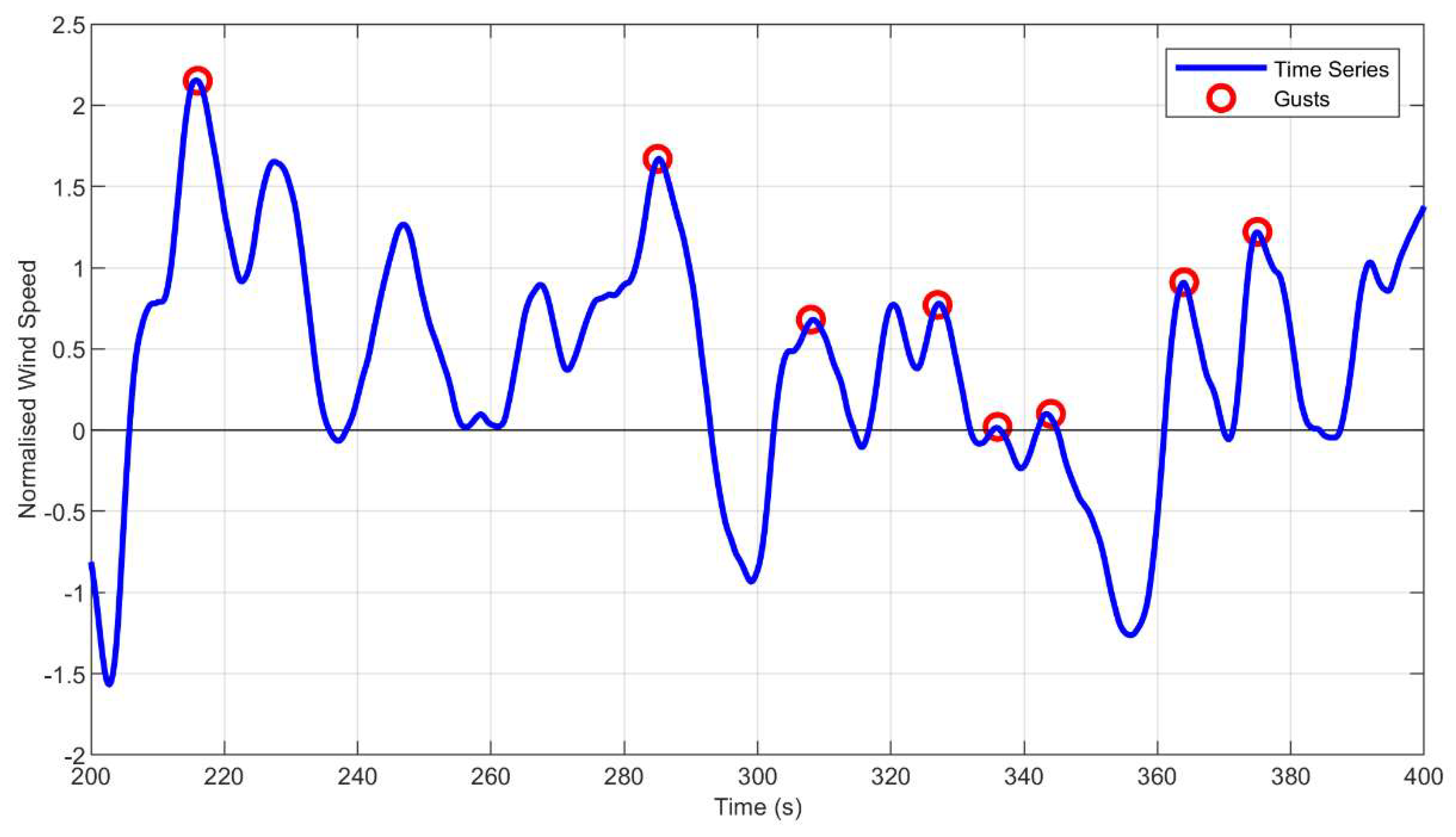
Figure 2.
Fits to normalized gust speeds in 60-minute record lengths.
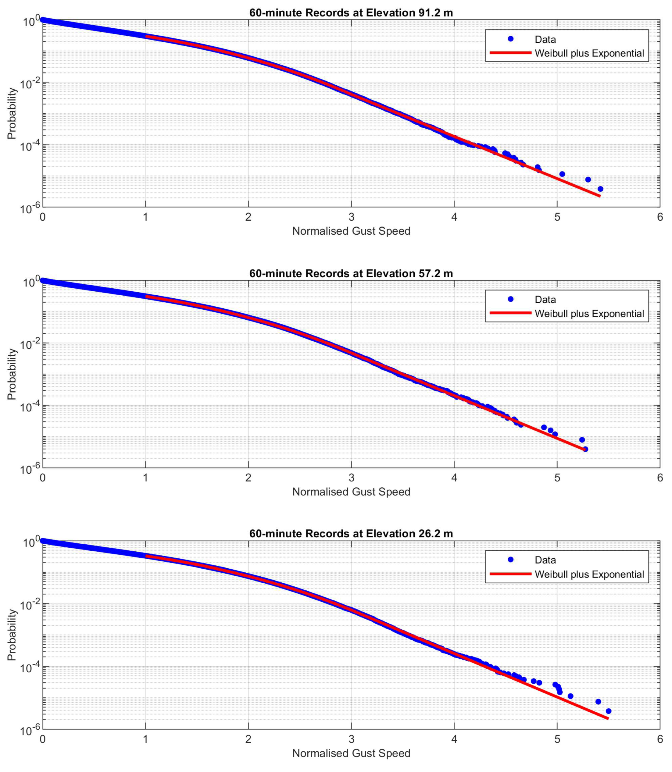
Figure 3.
Fits to normalized gust speeds in 10-minute record lengths.
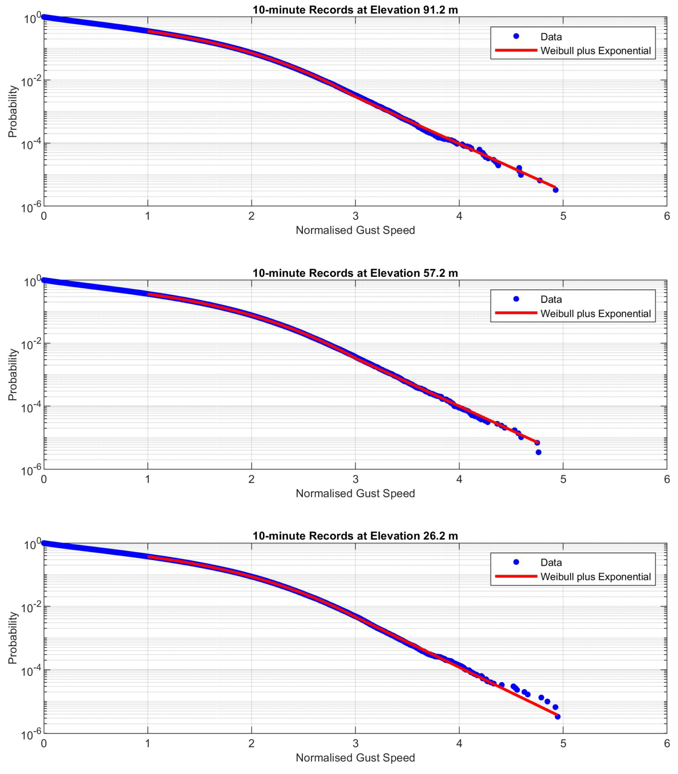
Figure 4.
Number of gusts in 60-minute records as a function of turbulence intensity.
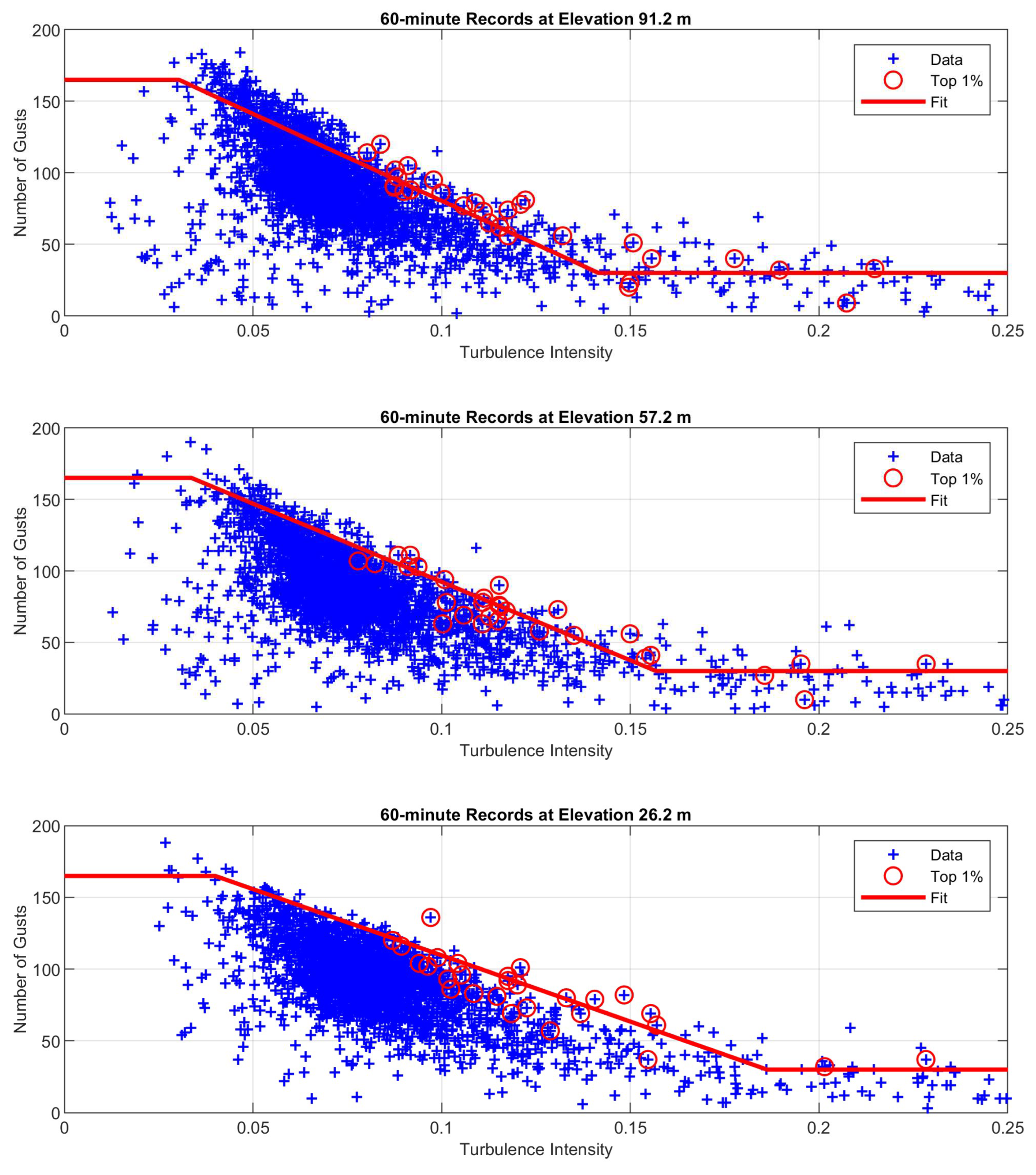
Figure 5.
Number of gusts in 10-minute records as a function of turbulence intensity.
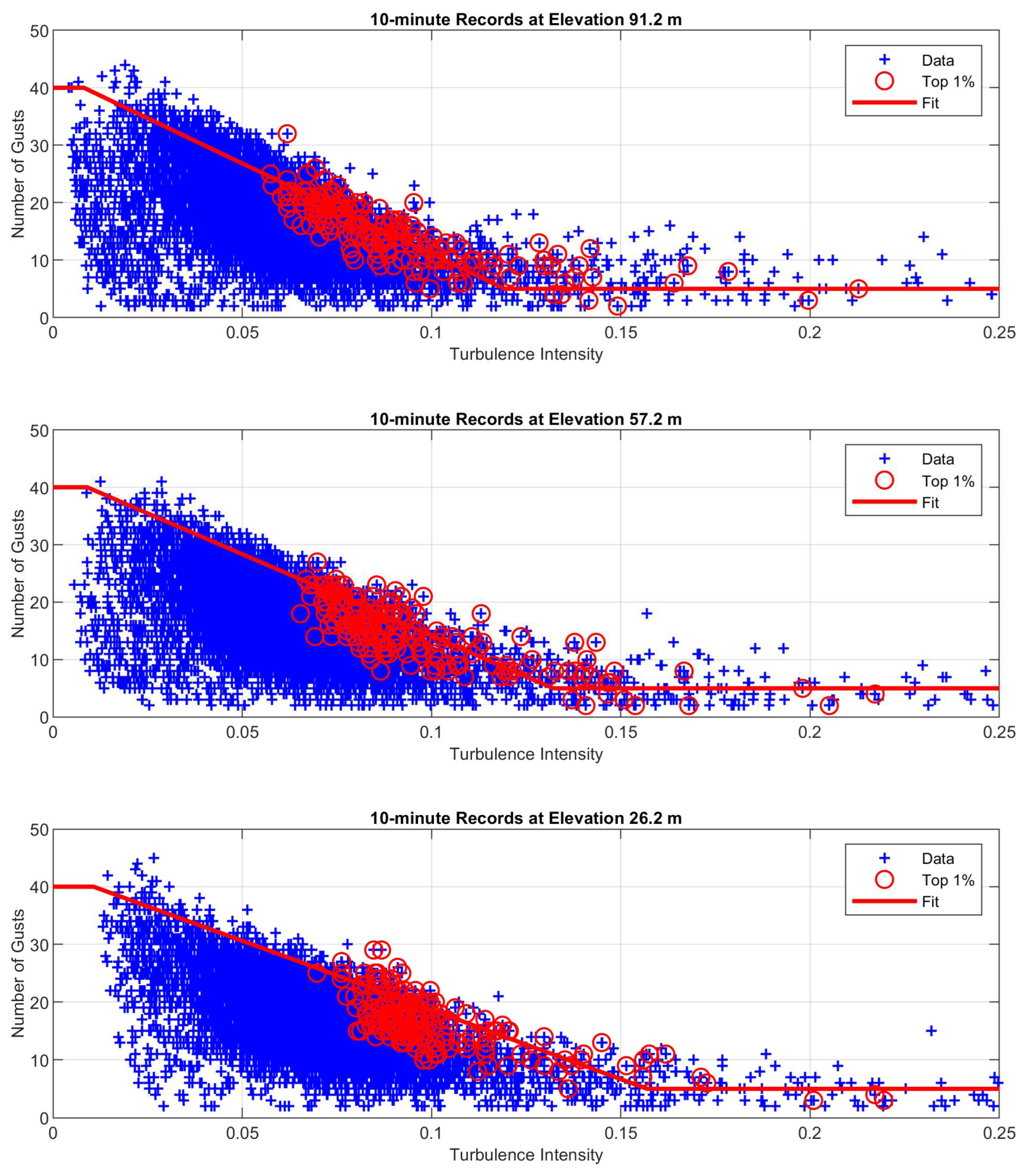
Figure 6.
Histograms of maximum dimensional gusts in 60-minute records.
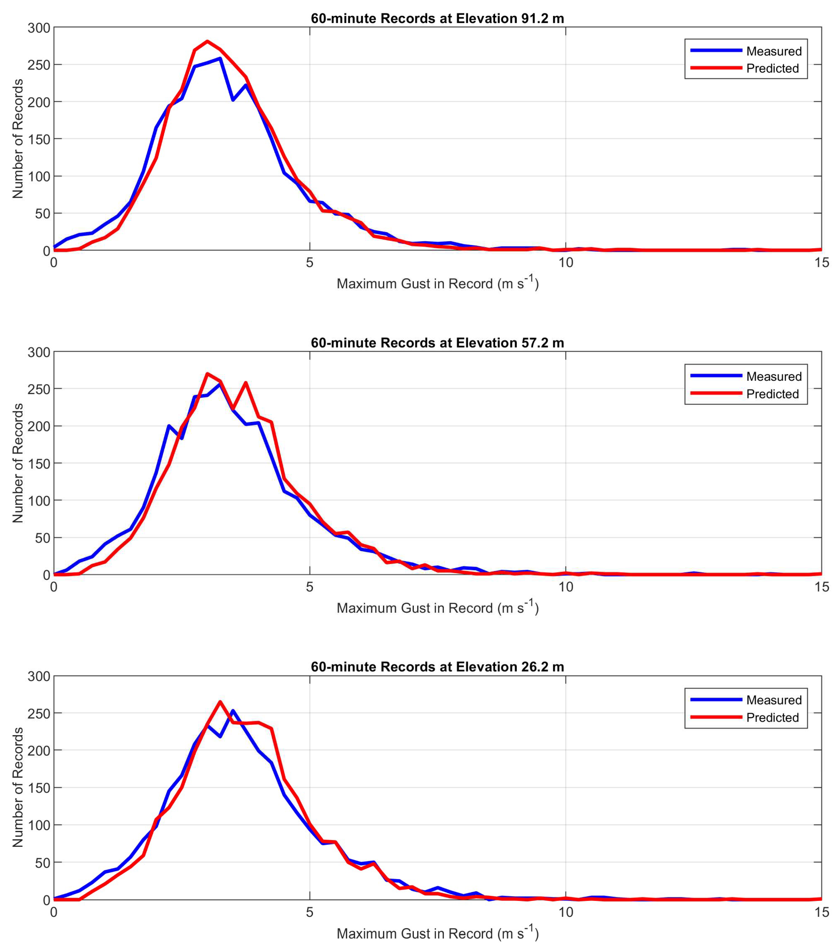
Figure 7.
Histograms of maximum dimensional gusts in 10-minute records.
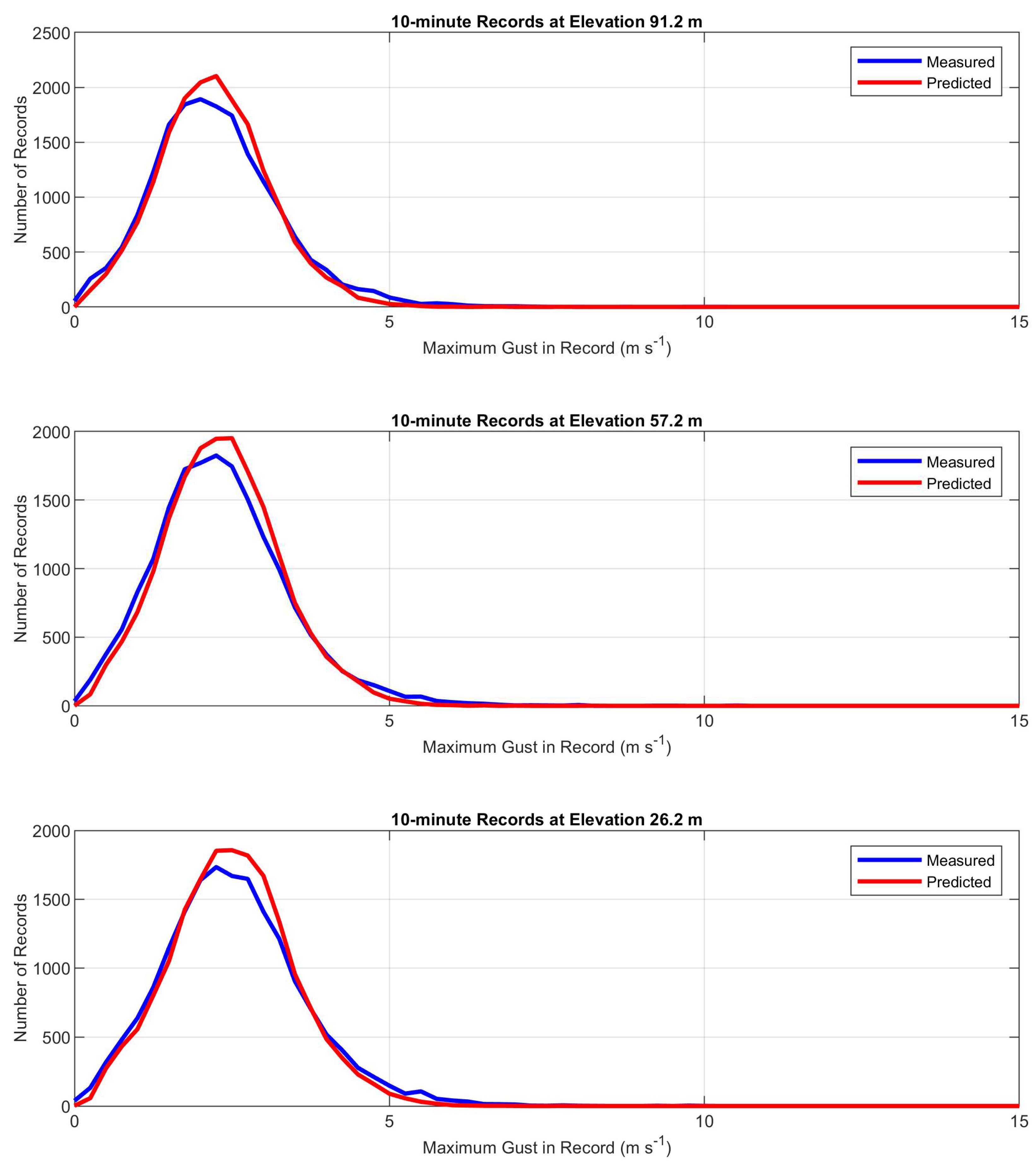
Figure 8.
Extreme value distributions of daily maximum dimensional total gust speeds from 60-minute records.
Figure 8.
Extreme value distributions of daily maximum dimensional total gust speeds from 60-minute records.
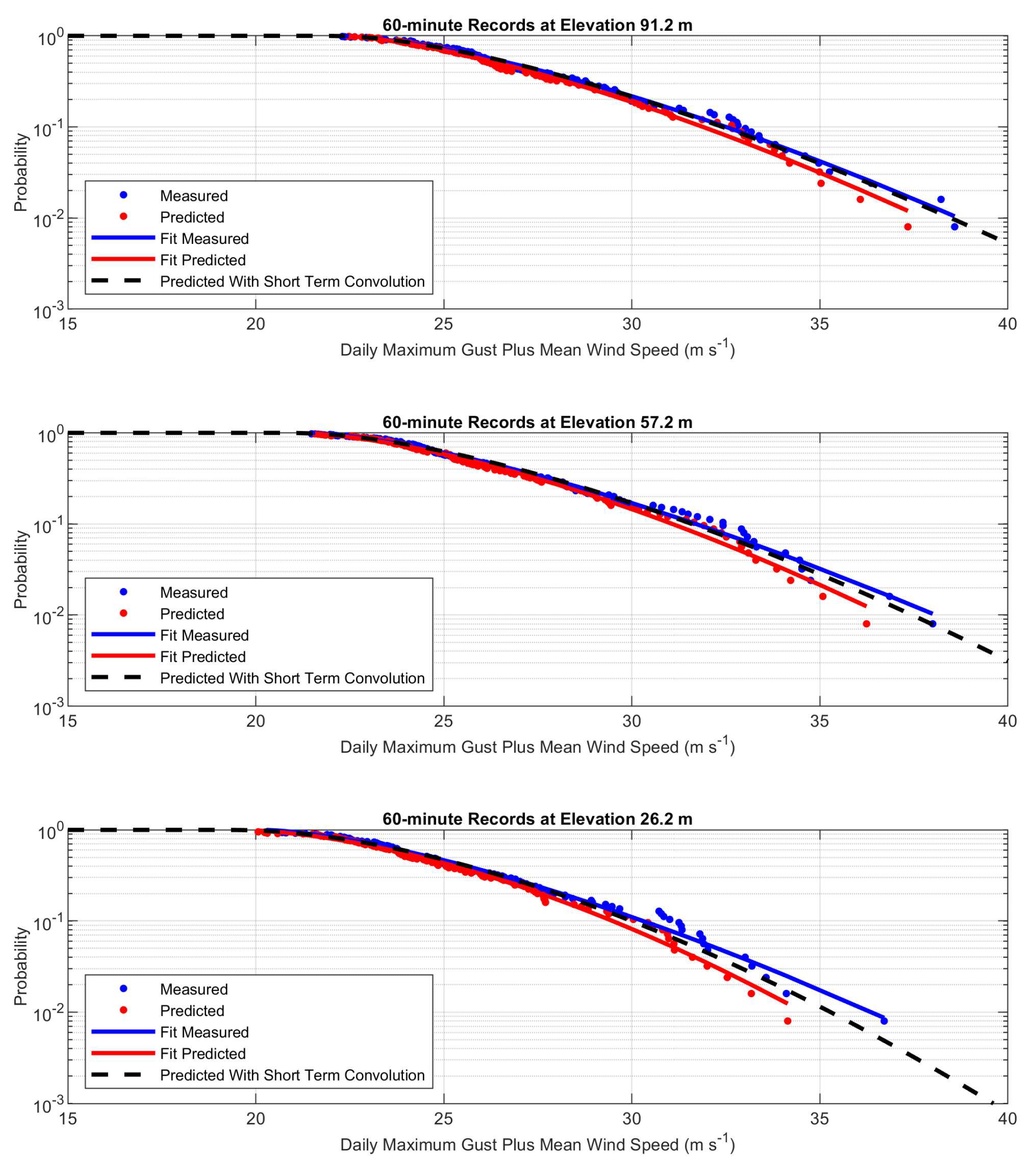
Figure 9.
Extreme value distributions of daily maximum dimensional total gust speeds from 10-minute records.
Figure 9.
Extreme value distributions of daily maximum dimensional total gust speeds from 10-minute records.
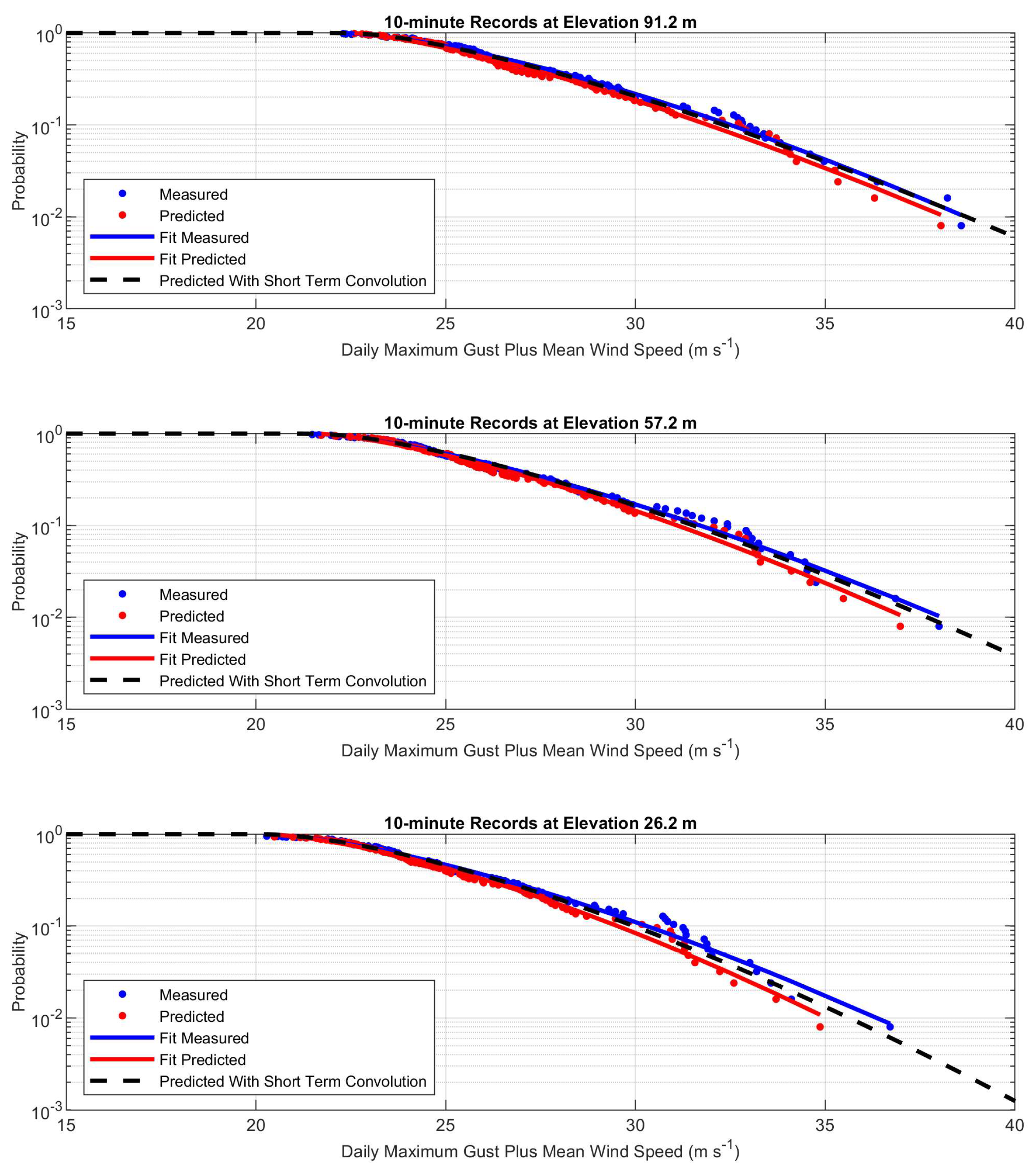
Figure 10.
Short term distributions of maximum gusts for 60-minute records.
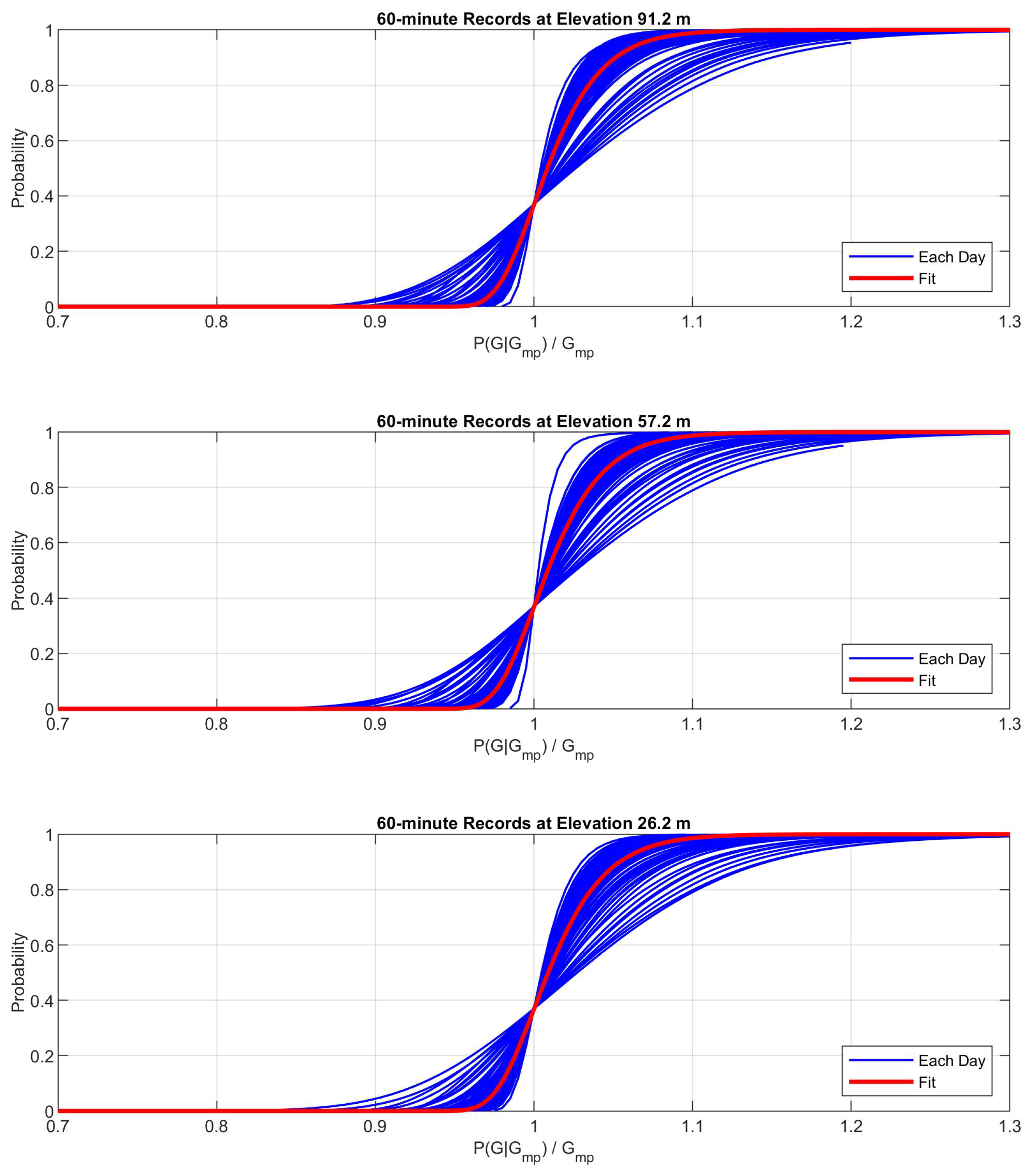
Figure 11.
Figure 11. Comparison of new extreme gust estimates and gust factors with ISO and IEC.
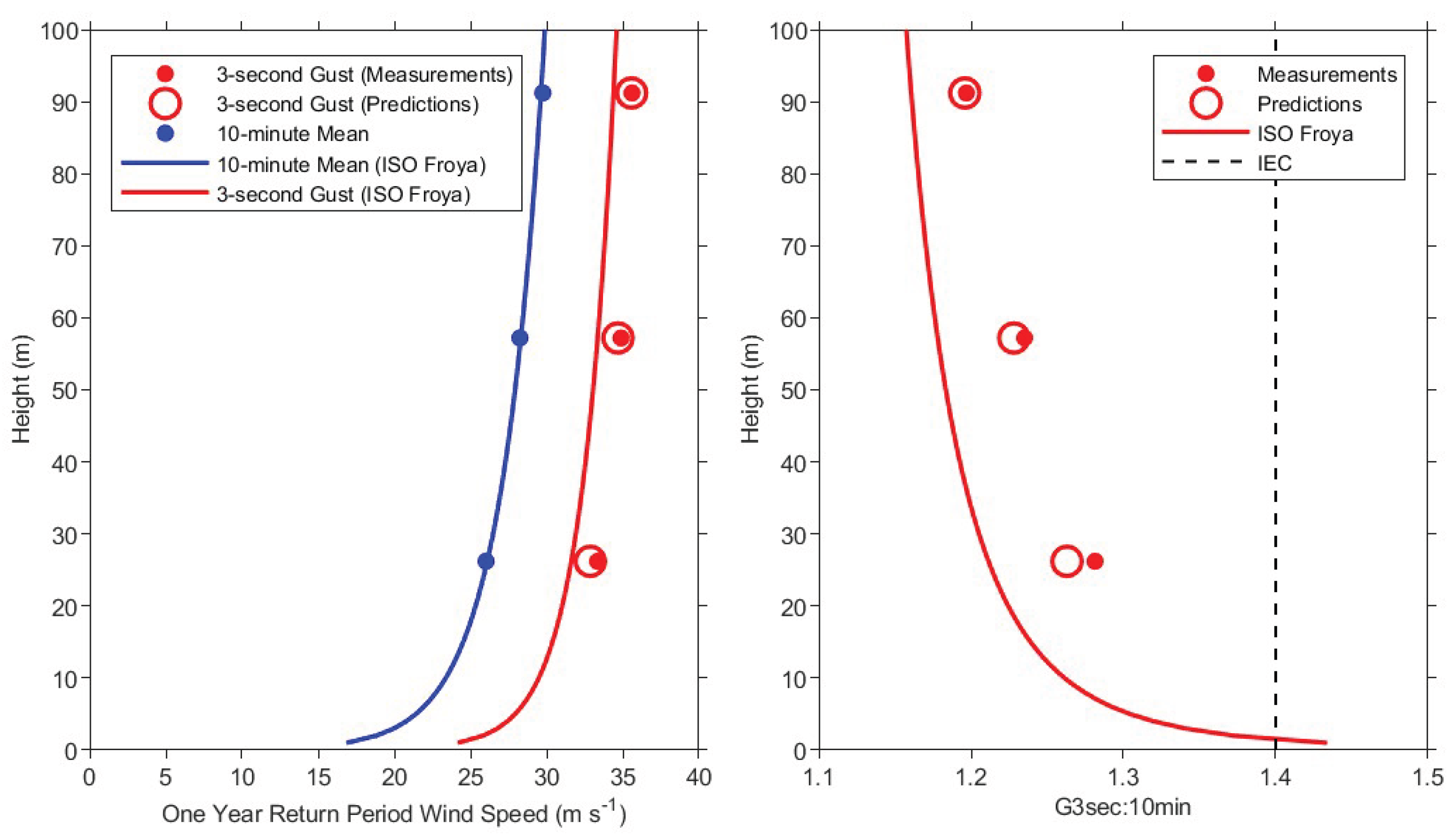

Table 1.
Coefficients in Equation (2) for each record length and elevation.
| Elevation (m) | Record Length (min) | α | β | γ | δ |
|---|---|---|---|---|---|
| 26.2 | 10 | 5.98 | 5.86 | -4.97 | 0.274 |
| 57.2 | 10 | 5.25 | 5.35 | -4.27 | 0.284 |
| 91.2 | 10 | 5.31 | 5.43 | -4.35 | 0.291 |
| 26.2 | 60 | 3.28 | 3.27 | -2.39 | 0.313 |
| 57.2 | 60 | 3.15 | 3.20 | -2.31 | 0.318 |
| 91.2 | 60 | 3.12 | 3.20 | -2.31 | 0.322 |
Table 2.
Estimates of extreme 3-second gusts from different methods.
| Elevation (m) | Record Length (Minutes) | Return Period (Years) | Measurements (m/s) |
Predictions Measured I(z) |
Predictions Predicted I(z) |
|---|---|---|---|---|---|
| 91.2 | 60 | 1 | 35.6 | 35.5 | 34.9 |
| 91.2 | 60 | 5 | 39.7 | 39.5 | 39.0 |
| 91.2 | 60 | 10 | 41.3 | 41.0 | 40.7 |
| 57.2 | 60 | 1 | 34.9 | 34.6 | 34.1 |
| 57.2 | 60 | 5 | 39.1 | 38.4 | 38.1 |
| 57.2 | 60 | 10 | 40.7 | 39.9 | 39.8 |
| 26.2 | 60 | 1 | 33.4 | 32.7 | 32.9 |
| 26.2 | 60 | 5 | 37.3 | 36.1 | 36.8 |
| 26.2 | 60 | 10 | 38.9 | 37.4 | 38.3 |
| 91.2 | 10 | 1 | 35.6 | 35.6 | 35.3 |
| 91.2 | 10 | 5 | 39.7 | 39.7 | 39.5 |
| 91.2 | 10 | 10 | 41.3 | 41.4 | 41.3 |
| 57.2 | 10 | 1 | 34.9 | 34.7 | 34.5 |
| 57.2 | 10 | 5 | 39.1 | 38.7 | 38.6 |
| 57.2 | 10 | 10 | 40.7 | 40.3 | 40.3 |
| 26.2 | 10 | 1 | 33.4 | 32.9 | 33.1 |
| 26.2 | 10 | 5 | 37.3 | 36.5 | 36.8 |
| 26.2 | 10 | 10 | 38.9 | 38.0 | 38.3 |
Disclaimer/Publisher’s Note: The statements, opinions and data contained in all publications are solely those of the individual author(s) and contributor(s) and not of MDPI and/or the editor(s). MDPI and/or the editor(s) disclaim responsibility for any injury to people or property resulting from any ideas, methods, instructions or products referred to in the content. |
© 2025 by the authors. Licensee MDPI, Basel, Switzerland. This article is an open access article distributed under the terms and conditions of the Creative Commons Attribution (CC BY) license (http://creativecommons.org/licenses/by/4.0/).
Copyright: This open access article is published under a Creative Commons CC BY 4.0 license, which permit the free download, distribution, and reuse, provided that the author and preprint are cited in any reuse.


