Submitted:
02 April 2025
Posted:
03 April 2025
You are already at the latest version
Abstract
Tidal storm surges can result in significant damage and inundation if sea defences are insufficiently robust. Calculation of flood risk enables coastal planners to site sea defences and coastal developments appropriately. Since the original work by Gumbel on extreme value statistics, several modifications and new methods have been proposed for the analysis of tidal inundation, with the Skew Surge Joint Probability Method (SSJPM) recently gaining popularity. However, SSJPM is complex, often requiring manual intervention, and is difficult to automate. Guided by the search for a method specifically applicable to tides that is amenable to automation, this paper proposes several modifications to Gumbel's original approach, including reducing the time unit for ranked maxima. This novel technique, here called TMAX, uses a time unit of one tidal-day, rather than the usual annual maxima (AMAX), to carry out an extreme-level analysis of recent tidal data at 35 United Kingdom coastal locations. The TMAX method gives a significantly better internal fit and reduced variance than the AMAX method and compared to a recent study using the SSJPM method at identical coastal locations, shows broad agreement, yet offers a considerably simpler implementation, amenable to automation. This new approach better informs strategies for coastal management and resilience.
Keywords:
Flood Return Period
; Tidal Flooding
; Coastal Flooding
; Sea level Rise
; Extreme Sea Level
1. Introduction
Coastal planners and developers require estimates of coastal flood risk so that sea defences, coastal buildings, harbours, nuclear power stations, and other infrastructure may be designed and located appropriately. Coastal floods generally occur when storm surges synchronize with high-tide overwhelming coastal sea defences. The frequency of such events has been predicted to double by 2050 because of rising sea levels (Vitousek et al.) while 68% of the global coastal area flooded will be caused by combined tide and storm events (Kirezki et al.) The potential impact of an increased risk of flooding will include loss of life, damage to infrastructure, coastal erosion, and loss of wetland habitat. The International Panel on Climate Change (IPCC 2021) estimates sea levels rose at 3.1 to 4.06 mm yr-1 from 2006 to 2015 with increases by 2100 anticipated between 0.28 to 1.01m depending upon the emissions scenario. The possibility of estimating the increased frequency of ESL events has been addressed by Wahl (2017) and Tebaldi (2021). It is important for such studies that the variation of ESL return period with height is known for each tidal location. The problem is acutely relevant in low-lying coastal countries, including parts of the United Kingdom (UK), Williams 2016. The required height of sea defences can vary quite rapidly along the coastline, because coastal topography may magnify or diminish tidal and surge effects. Coastal tide gauges are a useful source of input data for estimating flood probability and flood-return-period since they provide a local record from which the various flood risk parameters can be derived. This is a new use for tide-gauge data, it is generally used for tidal harmonic analysis, and establishment of tidal levels such as the Highest Astronomical Tide, HAT. Yet some man-made coastal structures may have a design life of hundreds or in the case of nuclear power stations, even thousands of years. The parameters required to characterize coastal flooding are different from those in harmonic analysis, since longer-term meteorological effects are included, rather than being excluded, as in tidal levels, such as HAT. Tide gauge data can reveal this flood risk, since it contains a "fingerprint" of past weather-induced extreme sea levels, Figure 1. During the past 60 years, many assessments of coastal flood risk in the UK were carried out, using several statistical methods, see UK Environment Agency (2011), Batstone (2013). This paper describes modifications to the AMAX method, including a change of the basic time window from years to tidal days; this is more than just a change of units, since the window forms an essential component of the statistical analysis. The study determines the flood return period as a function of height at 35 UK coastal tidal stations using the maximum sea level values each tidal day. The primary purpose of this study is to illustrate an application of the technique, rather than to provide a definitive re-appraisal of the UK flood defence heights.
Throughout this text, the term tide refers to the total sea level, while high tide refers to the peak events in total sea level. The astronomical tide refers to the deterministic component caused by tidal forces generated by the earth-solar and lunar-earth orbits. The difference between the total sea level and the astronomical tide is termed the residual component, principally caused by meteorological effects. The residual is also called the storm surge or random component.
2. Background
W.E. Fuller (1914) claimed that, on a purely empirical basis, the size of floods increases proportionately to the logarithm of time. Some 40 years later, Gumbel (1954) in his classic paper provided theoretical justification for Fuller's idea and gave many practical examples ranging from floods, radioactive decay, human life expectation, electrical capacitor breakdown, the strength of yarn, and the stock market. In Gumbel's original description, observed peak values, generally annual, were ranked in ascending order. Each ranked value i, was to be converted into the cumulative probability per unit time, Fi . After some deliberation, Gumbel in his Eq. (2.17) decided upon the formula
Fi = i / (N+1)
The probability (of a value not exceeding the ranked value) relates to the return period T (whose units are usually years) by Gumbel's Eq. (2.8), i.e.
T = 1/( 1 - Fi )
Gumbel showed that the probability of the value being below a given value could be written as
where the reduced variate, y linearly relates to the observed value x, via a scale factor α and location factor, μ and is given by
F(x) = exp( - exp( -y ))
y = α (x - μ)
In Gumbel's time, each ranked value was plotted on probability paper, where the horizontal scale had been marked out using Eq. (3), in terms of either return period or reduced variate, depending upon the manufacturer of the paper. A straight line was fitted to the points, and extrapolation of the line gave the probability of a value not exceedance for a given value x. Gringorten (1963) suggested a refinement of Eq. (1) which has been widely adopted as
F = ( i - 0.44) / ( N + 0.12 )
2.1. Subsequent Developments
The Gumbel Type I AMAX method uses only the largest annual extreme event, those events in second place or lower remain unused even if significant. To counter this apparent inefficient use of observed data, several techniques have been developed. The "r-largest" proposal (Smith 1986; Tawn 1988) uses a fixed number, r, of the largest annual maxima for analysis. Another proposal is the "peaks over threshold" (POT) method described by Coles (2001), whereby those maxima greater than a threshold value are used to create a new probability distribution. An earlier different approach (Pugh and Vassie 1978) split the total sea level into two components; the deterministic astronomical tide component and a random component. Each component was converted into separate probability distributions which were then combined using a convolution to produce a joint probability distribution. The method, known as the joint probability method (JPM) makes more efficient use of the source data and is widely used (McInnes et al. 2013), although its use has been criticised (Batstone et al. 2013). However, care must be taken to ensure the additive residual and astronomical components are sufficiently uncorrelated (Tawn and Vassie 1989; Tawn 1992). The correlation of the two components becomes especially apparent during storm surges because the time of high tide is often shifted in time relative to the underlying astronomical tide. The skew surge joint probability method, SSJPM, aimed to overcome this shortcoming by using the difference between the maxima, rather than the difference between instantaneous heights (Batstone et al. 2013). This difference, known as the "skew surge height", does not show such a correlation and is thus a suitable candidate for characterizing surge statistics. However, the number of values for extreme high tides is limited, resulting in a paucity of output points as compared to the JPM, thus requiring an extrema probability distribution such as the generalized Pareto distribution (GPD) to properly extrapolate the tail of the probability curve. The reader is referred to Batstone (2013) for the full system of equations. SSJPM was applied to tidal locations around the UK but Batstone reported: "At approximately one-quarter of the UKNTGN sites, it became clear that the GPD fitted on the skew surge distribution was leading to a seemingly implausible representation of the most extreme sea levels." The values were corrected by manual intervention using the AMAX method and also data values from nearby tidal stations. It has since been claimed that the deterministic astronomical tide and skew-surge have been proved to be truly independent, encouraging further work on this method (Williams et al. 2016). An important step in the extreme-level analysis is the determination of the quality of fit. A variety of methods of fit have been proposed and compared including the method of maximum likelihood (MML), method of moments (MOM), method of L-moments (MLM), method of probability-weighted moments (PWM), and the generalized least-squares methods GLSM/V. (Harris 1996, Coles 2000, Hong et al 2013).
3. Proposed TMAX Method
The proposed novel technique, named here TMAX, is designed to be accurate, to avoid manual intervention, to be relatively simple, to be suitable for automation, and to use the data more efficiently than the AMAX method. TMAX differs from the method described by Gumbel (and subsequently called AMAX) in three main ways. Firstly, a descending rank replaces the ascending order used by Gumbel. Secondly, a tidal day substitutes the annual grouping used in AMAX. Thirdly, only a subset n of the total N peak values is selected to fit a straight line. Further details are described below.
3.1. Descending Rank
We consider here F(x) to be the probability of the tide exceeding a height value x i.e. flood probability, rather than the opposite as in Gumbel's original formulation. Adding a prime to refer to the above equations Eqs. (2 & 3) from Gumbel's original paper and substituting for Gumbel's descending rank, i' with an ascending rank, i, where i = N + 1 - i' and F '= 1 - F, Eqs. (2 & 3) now become
Ti = 1 / Fi
F(x) = 1 - exp( - exp( -y ))
Neither the original rank formula Eq. (1) nor the Gringorten formula Eq. (5) requires correction since it can be shown by making the above substitutions that the formulae remain the same and hence apply to both ascending and descending ranks. The Gringorten formula, rather than Eq. (1), was used in all of the relevant calculations from hereon.
The inverse of Eq. (7) is used for readout purposes and is given by
yi = - loge( - loge( 1 - F(x) ))
As was pointed out by Gumbel, since F(x) is very small hence Eq. (8) approximates to y = log(T) confirming Fuller's original claim regarding how maximum flood height varies with time. The design risk D(x), i.e. the probability that a given value of x will be exceeded during a design life consisting of n durations (usually years), is given by
D(x) = 1 - ( 1- F(x) )n
3.2. Use of Tidal-Day as a Time Unit
Most but not all of the examples given by Gumbel use the annual maxima, which later became known as the AMAX method. However, in his original paper, Gumbel also examines some extreme events without using annualized data, such as the breaking point of yarn, and the breakdown voltage of electrical capacitors. He states in his conclusion, "If the number of observed extremes N is not excessive, do not group the observations." Therefore although extrema are often annually grouped before applying Gumbel's method it is not necessarily the case. This led the author to consider using a reduced time unit of one tidal day for the analysis. Changing the time unit from annual (AMAX) to tidal days (TMAX) ensures that if/when extremes occur within the same year, they are still utilized.
3.3. Selecting the Number of Peaks
In practice, as the data is scanned the peaks in each tidal day are determined and the largest peak is selected and stored. The set of peaks is then ranked with index 1 corresponding to the maximum of all of the peak values. Clearly, for a duration of tidal data of years or decades, there will be many thousands of tidal-daily peak values. Of these N peaks, we use only the n largest values, where n is calculated from an average number required per year na multiplied by the duration in years ny, i.e. n = na x ny. The number of points used for the line fit is thus much smaller than the number of maxima. This avoids the fit from being affected by any curvature in the extreme distribution at the smaller peak values since these are more likely to occur when the smaller deterministic tides (neap tides) combine with smaller values of surge, rather than the higher values of both. The total number of values N is taken to be the number of tidal days and is given by the data duration divided by the duration of a tidal day (in the same units). The symbol 'i' still corresponds to the index of the ranked maxima in Eqs. (1 & 5). The optimization of na is described subsequently in Section 4.1. Note that this proposed method is quite different from the Points Over Threshold (POT) method, where the wings of an upper section of a probability distribution function are fitted to a standard distribution such as a Generalised Pareto Distribution (GPD). Here in the TMAX method, like in Gumble, ranking is used to determine the probability.
3.4. Straight Line Fit
The ordinary least squares (LSQ) method, also known as linear regression was used to determine the line fit (Morrison 2021). Although other methods are available (see 2.1 above), the LSQ method is used here as a proof of concept of the TMAX algorithm. Furthermore, the slope, intercept, and variance of the mean and predicted with LSQ are represented by simple closed-loop expressions. Consideration of other fitting methods with TMAX may be viewed as a potential refinement for future research. With both AMAX and TMAX methods, the expected value of a predicted new point (i.e. a flood) is the mean y value of the intersection of the extrapolated regression line with the ordinate corresponding to the return period, see Figure 2. Just as with the standard Gumbel method, the main drawback is the requirement for the extrapolation of the regression line away from the mean values of x, the accuracy worsening with short durations of tidal data. Although the mean of the intersection points and the new predicted value are identical they have different uncertainties. Morrison gives expressions for the variance of the mean value σm and the variance of the predicted new value σp below, where n represents the number of data points, xm, and ym are the mean x and y values respectively.
where s2y,x = ( 1/(n-2) ) Σ(yi - ym)2
σm = s2y,x ( 1/n + (xp - xm)2 / SSxx )
σp = s2y,x (1 + 1/n + (xp - xm)2/SSxx)
SSxx = Σ(xi - xm)2
The variance of the new predicted point mean is always greater than the variance of the mean; practically this is because a new point is subjected to variation in the process, whereas the variance in the intersection is subject to variation in the regression line parameters, the latter tending towards zero as the number of data points increases.
3.5. Missing Data
Missing observed data using the TMAX method can simply be taken into account by reducing the duration to include only periods of valid data. By contrast, in the AMAX method handling missing data is not so straightforward, since either synthetic data must be provided to fill the gaps, (as was discussed by Gumbel), or entire years of data must be rejected if the data content is below a given threshold, say 90%. In this study, the latter technique was used for the AMAX method.
4. Methodology
The study is based on data from the same 35 UK stations as were used by Batstone. This data was downloaded and manually inspected, and isolated non-contiguous data points and points showing clear evidence of gauge slips were removed. All data was sea-level rise de-trended, using either the constant figure adopted by Batstone of 2mm per year or the intrinsic rate of sea level rise recorded. In the latter case sea level rise was calculated by linear regression on the maximum number of whole tidal cycles. The de-trending was arranged to apply a zero correction on 1 January 2008, to facilitate comparison with the results from Batstone who used the same date origin. Most data before 1993 had been recorded at hourly intervals whereas subsequently, data was at 15-minute intervals. To obtain the longest data duration possible, both 15-minute and one-hourly data were used within a single file for many of the locations. Although there is a risk that the use of hourly data may result in missing or under-recording of the true peak value, most significant surges are at least one hour in duration, reducing this likelihood. The advantage of using much longer records should therefore easily outweigh the potential small inaccuracy due to the change in sample rate within the file. Each high tide was determined by ensuring that the central point was greater than its neighbouring points. At most, each high tide must count as a single flood surge event, hence a check was made to examine whether more than one high tide occurred within 12 hours, if the curve contained more than one high tide within this time window the larger of the maxima was used, and the smaller was rejected. In the first phase of analysis, the optimum value of nA was determined using the data processed above. In the second phase, the extreme sea levels corresponding to a given return period were determined. These phases are now described and comparisons with the results from Batstone are indicated where appropriate.
4.1. Optimising the Average Number of Peaks Per Year, na
As discussed above, larger values of na cause a higher proportion of peaks to originate from smaller astronomical tides (neap tides). Therefore, although smaller values of na generally are associated with an increase in the variance, smaller values may decrease the dependence upon the smaller deterministic neap-tides improving the accuracy. Figure 3 shows how in practice the variance of the mean, σm, and variance of a predicted new point, σp vary with na, the average number of extremes selected per year, using the TMAX method. The values were determined from the tidal data using Eqs. (10 & 11). The variance of the mean, σm decreases as na increases; however, σp shows a minimum with a value of na of around five extremes per year. This concurs with the value of five per year recommended for extreme river flow studies, (see Robson and Reed 1999 using the different Peaks-Over-Threshold POT method, although this may be coincidental. Nevertheless, since it shows a minimum variance, the value na = 5 was used for all subsequent results. Table 1 illustrates the quality of fit of the regression lines for the two data durations and the AMAX and TMAX methods. The TMAX method, as compared to AMAX, gave a higher quality of fit. The AMAX method showed a variance of the mean flood height value of around ±0.1 meters and a variance of a predicted new value of around ±0.4 meters, while the TMAX method gave lower values at around ±0.03 meters and ±0.24 meters respectively.
4.2. Determination of Extreme Sea Levels
Figure 2 shows a typical Gumbel plot for a single location, Heysham. The corresponding top four plotted points/heights are also listed in Table 2. All of the results were derived directly from the tide gauge data and have not been re-processed in any way to enforce the agreement with any other data set or with neighbouring local values. The analysis was carried out for the entire data set consisting of 35 ports, once with the tidal records truncated to 1 Jan 2009 for comparison with the results of Batstone's analysis, and once using the complete data set to 1 May 2018. Each data set was analyzed using the AMAX and TMAX methods. Each study applied Sea-level rise de-trending at 2mm per year with a date origin of 2008. The analysis used Gringorten's correction throughout for compatibility with Batstone's research.
Table 3 compares the AMAX and TMAX results with those of Batstone. The mean differences for data to 2009 using either method were generally in the centimetre region. In either case, the standard deviation was around 0.1m rising to approximately 0.24m for the 1000-year return level and was somewhat higher for the AMAX than for TMAX. Figure 4 shows the frequency distribution of the differences between TMAX results derived from data to 2009 and data to 2018 across the 35 UK ports, showing a rise in level for each return period T.
Table 4 indicates an average rate of rise over the 9 years of the extreme 20-year sea level of 3.4x10⁻³ yr-1 and for the 1000-year level of 6.1x10⁻³ yr-1. This compares with a rate of rise calculated for the whole dataset of 1.85x10⁻³ yr-1. When the increase is analyzed by the paired-sample left-tailed t-test it gives P values of 0.005 to 0.006 indicating the increase in level is significant.
The figures for sea level rate of rise do not include glacial isostatic adjustment (GIA) or geoid adjustments and are reasonably in line with reported values, (Wahl et al. 2013; Church and White 2011, IPCC 2021). Table 5 shows the heights using the TMAX method corresponding to the return periods of 20, 100, 200, and 1000 years for the 35 locations; it also lists the differences from Batstone's results. Figure 5 shows the ESL values for a 100-year return period deduced by the TMAX using the data to 2018. The colours indicate whether the values are higher (red) or lower (green) compared with the TMAX analysis to 2009. Investigation of the individual contributing tidal locations reveals four main outliers when comparing this 2018 TMAX study to Batstone's results for the 200-year return period (with heights shown in brackets) are; Tobermory (-0.3), Avonmouth (-0.26), Holyhead (0.37), Immingham (0.24). Attention is drawn to these locations as their ESLs may require revision.

Table 5.
Extreme Sea-level (ESL) at UK coastal locations calculated from data to 2018 using TMAX method. The differences listed are relative to Batstone 2013 using data to 2009. Heights are in meters above Ordnance Datum Newlyn (ODN), relative to the mean sea level on 1 January 2008.
Table 5.
Extreme Sea-level (ESL) at UK coastal locations calculated from data to 2018 using TMAX method. The differences listed are relative to Batstone 2013 using data to 2009. Heights are in meters above Ordnance Datum Newlyn (ODN), relative to the mean sea level on 1 January 2008.
| Data | Return Period (yrs) | Difference from Batstone (m) | |||||||
| Location | Days | 20 | 100 | 200 | 1000 | D20 | D100 | D200 | D1000 |
| Aberdeen | 8798 | 2.99 | 3.14 | 3.20 | 3.35 | 0.02 | 0.03 | 0.03 | 0.06 |
| Avonmouth | 6227 | 8.53 | 8.75 | 8.85 | 9.08 | -0.14 | -0.23 | -0.26 | -0.35 |
| Barmouth | 8497 | 3.88 | 4.08 | 4.16 | 4.36 | -0.04 | -0.05 | -0.06 | -0.05 |
| Bournemouth | 6292 | 1.68 | 1.84 | 1.91 | 2.08 | 0.00 | 0.03 | 0.04 | 0.09 |
| Dover | 22578 | 4.35 | 4.62 | 4.74 | 5.01 | 0.11 | 0.14 | 0.17 | 0.21 |
| Felixstowe | 6384 | 3.27 | 3.59 | 3.72 | 4.03 | -0.06 | -0.13 | -0.18 | -0.34 |
| Fishguard | 13974 | 3.38 | 3.52 | 3.58 | 3.73 | 0.01 | 0.00 | 0.00 | 0.00 |
| Heysham | 17834 | 6.34 | 6.59 | 6.70 | 6.95 | -0.08 | -0.11 | -0.12 | -0.14 |
| Hinkley Point | 9077 | 7.41 | 7.57 | 7.64 | 7.81 | -0.10 | -0.17 | -0.20 | -0.28 |
| Holyhead | 15488 | 3.90 | 4.15 | 4.26 | 4.52 | 0.22 | 0.32 | 0.37 | 0.48 |
| Immingham | 20895 | 4.80 | 5.11 | 5.24 | 5.55 | 0.16 | 0.22 | 0.24 | 0.30 |
| Kinlochbervie | 7754 | 3.70 | 3.94 | 4.04 | 4.28 | 0.09 | 0.10 | 0.10 | 0.11 |
| Leith | 8453 | 3.67 | 3.81 | 3.87 | 4.02 | -0.02 | -0.07 | -0.10 | -0.18 |
| Lerwick | 12104 | 1.75 | 1.88 | 1.93 | 2.06 | 0.02 | 0.05 | 0.06 | 0.11 |
| Llandudno | 8046 | 5.10 | 5.30 | 5.38 | 5.58 | 0.01 | 0.01 | 0.00 | 0.00 |
| Lowestoft | 19538 | 2.69 | 3.07 | 3.23 | 3.60 | 0.04 | 0.00 | -0.04 | -0.18 |
| Milford Haven | 18158 | 4.57 | 4.75 | 4.83 | 5.02 | 0.09 | 0.08 | 0.08 | 0.07 |
| Millport | 12422 | 3.26 | 3.55 | 3.67 | 3.96 | 0.06 | 0.03 | 0.00 | -0.07 |
| Moray Firth | 3127 | 3.22 | 3.36 | 3.41 | 3.54 | 0.09 | 0.07 | 0.06 | 0.03 |
| Mumbles | 6121 | 5.85 | 6.03 | 6.11 | 6.30 | 0.02 | -0.02 | -0.04 | -0.09 |
| Newhaven | 11184 | 4.12 | 4.26 | 4.32 | 4.47 | -0.07 | -0.11 | -0.13 | -0.17 |
| Newlyn | 37171 | 3.43 | 3.59 | 3.66 | 3.81 | 0.10 | 0.13 | 0.15 | 0.18 |
| Newport | 8854 | 8.00 | 8.20 | 8.28 | 8.47 | 0.00 | -0.08 | -0.13 | -0.25 |
| North Shields | 18275 | 3.69 | 3.93 | 4.03 | 4.27 | 0.14 | 0.17 | 0.17 | 0.16 |
| Portpatrick | 17490 | 3.26 | 3.47 | 3.57 | 3.79 | 0.07 | 0.10 | 0.12 | 0.18 |
| Portsmouth | 8561 | 2.88 | 3.03 | 3.10 | 3.25 | 0.00 | -0.02 | -0.02 | -0.03 |
| Port Ellen | 6576 | 1.73 | 1.95 | 2.05 | 2.27 | -0.20 | -0.19 | -0.17 | -0.14 |
| Sheerness | 15999 | 4.21 | 4.45 | 4.56 | 4.80 | 0.08 | -0.02 | -0.08 | -0.25 |
| Stornoway | 12709 | 3.25 | 3.43 | 3.50 | 3.67 | 0.04 | 0.09 | 0.10 | 0.15 |
| Tobermory | 7890 | 3.32 | 3.50 | 3.57 | 3.75 | -0.15 | -0.24 | -0.30 | -0.43 |
| Ullapool | 16051 | 3.65 | 3.84 | 3.92 | 4.11 | 0.06 | 0.08 | 0.10 | 0.15 |
| Weymouth | 8739 | 2.13 | 2.27 | 2.32 | 2.45 | 0.08 | 0.07 | 0.06 | 0.05 |
| Whitby | 13192 | 3.70 | 3.89 | 3.97 | 4.16 | -0.08 | -0.13 | -0.17 | -0.25 |
| Wick | 18173 | 2.75 | 2.90 | 2.97 | 3.12 | 0.06 | 0.07 | 0.08 | 0.09 |
| Workington | 9017 | 5.66 | 5.91 | 6.02 | 6.28 | 0.10 | 0.10 | 0.11 | 0.13 |
| Mean | 0.02 | 0.01 | 0.00 | -0.02 | |||||
| Stdev | 0.09 | 0.12 | 0.14 | 0.20 | |||||
5. Conclusion
The results indicate that the proposed TMAX method, as implemented above, when applied to UK tide gauge data, generates reasonable estimates of ESL flood defence height, broadly in agreement with published values (UK Environment Agency 2011), with mean differences of the order of centimetres and standard deviation of the order of decimetres. However, the TMAX method is much simpler than the SSJPM used in EA2011. TMAX, like the Gumbel method, relies solely on ranking (although it contains a points over threshold concept), and unlike the SSJPM it does not use or require a) harmonic tidal analysis, b) the use of a probability density function, or c) the fit of a generalized Pareto distribution (GPD). Compared to the well-known annual grouping AMAX method, the TMAX method gives a significantly better internal fit and reduced variance in new predicted values. Furthermore, unlike the SSJPM, it was not necessary to intervene manually. The TMAX method is amenable to automation and is suitable for extreme coastal sea level analysis. This innovative approach enhances our understanding of sea-level fluctuations and more effectively informs strategies for coastal management and resilience.
Acknowledgments
The author is grateful to the British Oceanographic Data Centre (BODC), who provided the tidal data used in this research via their "Sea Level Portal" at https://www.bodc.ac.uk. BODC do not accept any liability for the correctness and/or appropriate interpretation of the data or their suitability for any use. This study was independently undertaken using additions to the tidal harmonic analysis system GeoTide developed by Geomatix Ltd, UK of which the author is the managing director. The TMAX algorithm is copyright of Geomatix Ltd, UK ©2022.
References
- Batstone, C., Lawless, M., Tawn, J., Horsburgh, K., Blackman, D., McMillan, A., Worth, D., Laeger, S., Hunt, T., 2013. A UK best-practice approach for extreme sea-level analysis along complex topographic coastlines. Ocean Engineering 71, 28–39. [CrossRef]
- Church, J.A., White, N.J., 2011. Sea-Level Rise from the Late 19th to the Early 21st Century. Surv Geophys 32, 585–602. [CrossRef]
- Coles, S.G., Dixon, M.J., 2000. Likelihood-Based Inference for Extreme Value Models. Extremes 2, 5–23. [CrossRef]
- Coles, S., 2001. An Introduction to Statistical Modeling of Extreme Values, Springer Series in Statistics. Springer London, London. [CrossRef]
- Fuller, W.E., 1914 Flood flows, Trans. A. S. C. E. Paper 1293, LXXVII, 564 (1914).
- Gringorten, I.J., 1963. A Plotting Rule for Extreme Probability Paper. Journal of Geophysical Research Vol68 No 3 February 1, 1963.
- Gumbel, E.J., Lieblein, J., 1954 "Statistical Theory of Extreme Values and Some Practical Applications: A Series of Lectures (Vol. 33)". 1954. National Bureau of Standards, US Government Printing Office, Washington.
- Harris, R. I. (1996). Gumbel re-visited - a new look at extreme value statistics applied to wind speeds. Journal of Wind Engineering and Industrial Aerodynamics, 59(1), 1–22. [CrossRef]
- Hong, H.P., Li, S.H., Mara, T.G., 2013. Performance of the generalized least-squares method for the Gumbel distribution and its application to annual maximum wind speeds. Journal of Wind Engineering and Industrial Aerodynamics 119, 121–132. [CrossRef]
- IPCC 2021: Climate Change 2021: The Physical Science Basis. Contribution of Working Group I to the Sixth Assessment Report of the Intergovernmental Panel on Climate Change. Cambridge University Press, UK & NY, USA. [CrossRef]
- Kirezci, E., Young, I.R., Ranasinghe, R. et al. Projections of global-scale extreme sea levels and resulting episodic coastal flooding over the 21st Century. Sci Rep 10, 11629 (2020). [CrossRef]
- McInnes, K.L., Macadam, I., Hubbert, G., O’Grady, J., 2013. An assessment of current and future vulnerability to coastal inundation due to sea-level extremes in Victoria, southeast Australia: Current And Future Coastal Inundation In Victoria, Australia. Int. J. Climatol. 33, 33–47. [CrossRef]
- Morrison, F.A., 2020. Uncertainty Analysis for Engineers and Scientists: A Practical Guide, 1st ed. Cambridge University Press. [CrossRef]
- Pugh, D.T., Vassie, J.M., Extreme Sea Levels from Tide and Surge Probability. 1978. Coastal Engineering 1978: 911-930.
- Robson, A., Reed,D., 1999. Flood Estimation Handbook Volume 3. Statistical procedures for flood frequency estimation. ISBN: 978-1-906698-03-4. Institute of Hydrology 1999.
- Smith, R.L., 1986. Extreme value theory based on the r largest annual events. Journal of Hydrology 86, 27–43. [CrossRef]
- Tawn, J.A., 1988, An extreme-value theory model for dependent observations. Journal of Hydrology 101, 227-250.
- Tawn, J.A., Vassie, J.M., 1989. Extreme Sea Levels: The Joint Probabilities Method Revisited and Revised. Proc. Inst. Civ. Engrs. Part 2, 87, Sept., 429-442. [CrossRef]
- Tawn, J.A., 1992. Estimating Probabilities of Extreme Sea-Levels. Applied Statistics 41, 77. [CrossRef]
- Tebaldi, C., Ranasinghe, R., Vousdoukas, M., Rasmussen, D.J., Vega-Westhoff, B., Kirezci, E., Kopp, R.E., Sriver, R., Mentaschi, L., 2021. Extreme sea levels at different global warming levels. Nat. Clim. Chang. 11, 746–751. [CrossRef]
- UK Environment Agency 2011. Coastal flood boundary conditions for UK mainland and islands, Project: SC060064/TR2: Design sea levels, Environment Agency UK. ISBN 978-1-84911-212-3, © Environment Agency. February 2011.
- Vitousek, S., Barnard, P., Fletcher, C. et al. Doubling of coastal flooding frequency within decades due to sea-level rise. Sci Rep 7, 1399 (2017). [CrossRef]
- Wahl, T., Haigh, I.D., Woodworth, P.L., Albrecht, F., Dillingh, D., Jensen, J., Nicholls, R.J., Weisse, R., Wöppelmann, G., 2013. Observed mean sea level changes around the North Sea coastline from 1800 to present. Earth-Science Reviews 124, 51–67. [CrossRef]
- Wahl, T., Haigh, I.D., Nicholls, R.J., Arns, A., Dangendorf, S., Hinkel, J., Slangen, A.B.A., 2017. Understanding extreme sea levels for broad-scale coastal impact and adaptation analysis. Nat Commun 8, 16075. [CrossRef]
- Williams, J., Horsburgh, K.J., Williams, J.A., Proctor, R.N.F., 2016. Tide and skew surge independence: New insights for flood risk: Skew Surge-Tide Independence. Geophys. Res. Lett. 43, 6410–6417. [CrossRef]
Figure 1.
Tidal height (black) and residual (red) showing extreme sea level on 5 Dec 2013, Whitby, UK.
Figure 1.
Tidal height (black) and residual (red) showing extreme sea level on 5 Dec 2013, Whitby, UK.
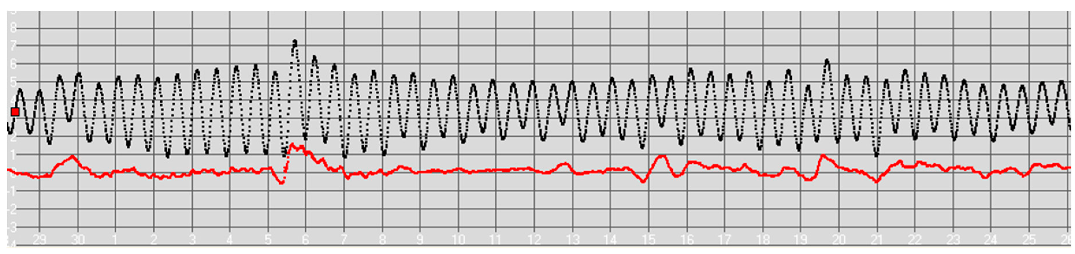
Figure 2.
The mean-variance σm and of the predicted new point variance σp plotted against the number of extrema per year Na for the TMAX method as determined from the tidal data.
Figure 2.
The mean-variance σm and of the predicted new point variance σp plotted against the number of extrema per year Na for the TMAX method as determined from the tidal data.
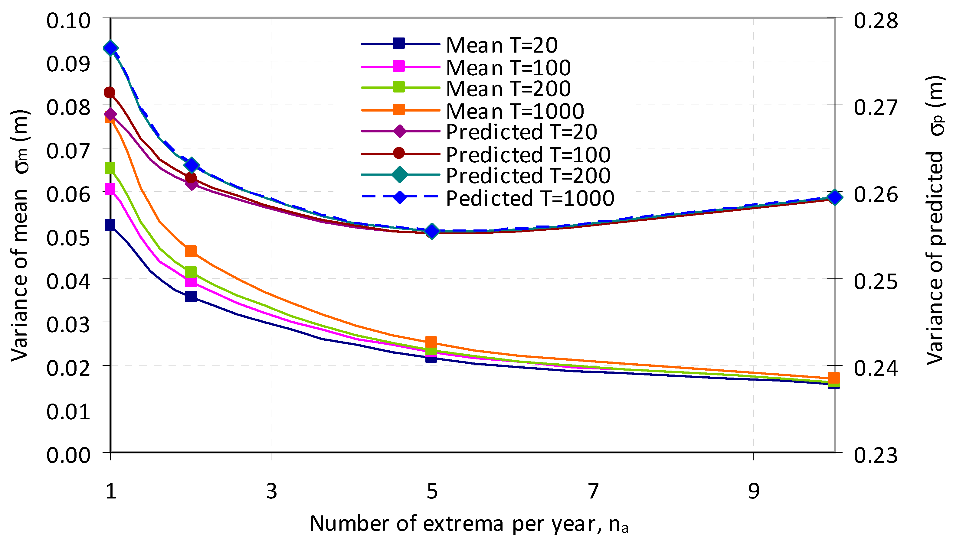
Figure 3.
Gumbel plot of 242 highest tides at Heysham, showing regression line, reduced variate x-axis, and height in meters relative to input datum Admiralty Chart Datum (ACD). OSDN-CD Heysham=4.9m. 200-year flood return height is 11.6m (CD) - 4.9m(OSDN-CD) = 6.7m (OSDN). See Table 5.
Figure 3.
Gumbel plot of 242 highest tides at Heysham, showing regression line, reduced variate x-axis, and height in meters relative to input datum Admiralty Chart Datum (ACD). OSDN-CD Heysham=4.9m. 200-year flood return height is 11.6m (CD) - 4.9m(OSDN-CD) = 6.7m (OSDN). See Table 5.
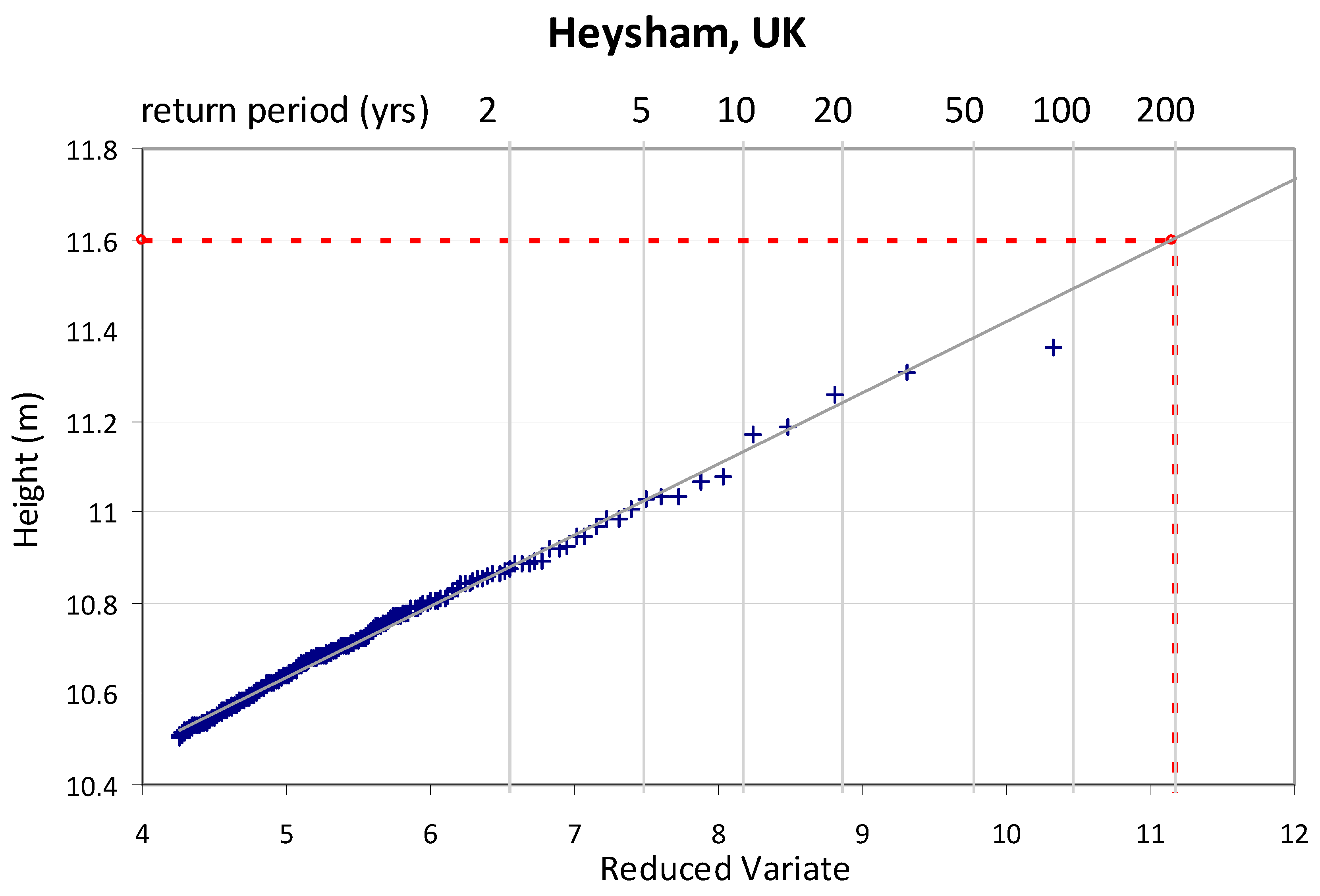
Figure 4.
Number of ports showing a given rise in the level of the return period between data to 2009 and data to 2018 as analyzed across 35 UK ports.
Figure 4.
Number of ports showing a given rise in the level of the return period between data to 2009 and data to 2018 as analyzed across 35 UK ports.
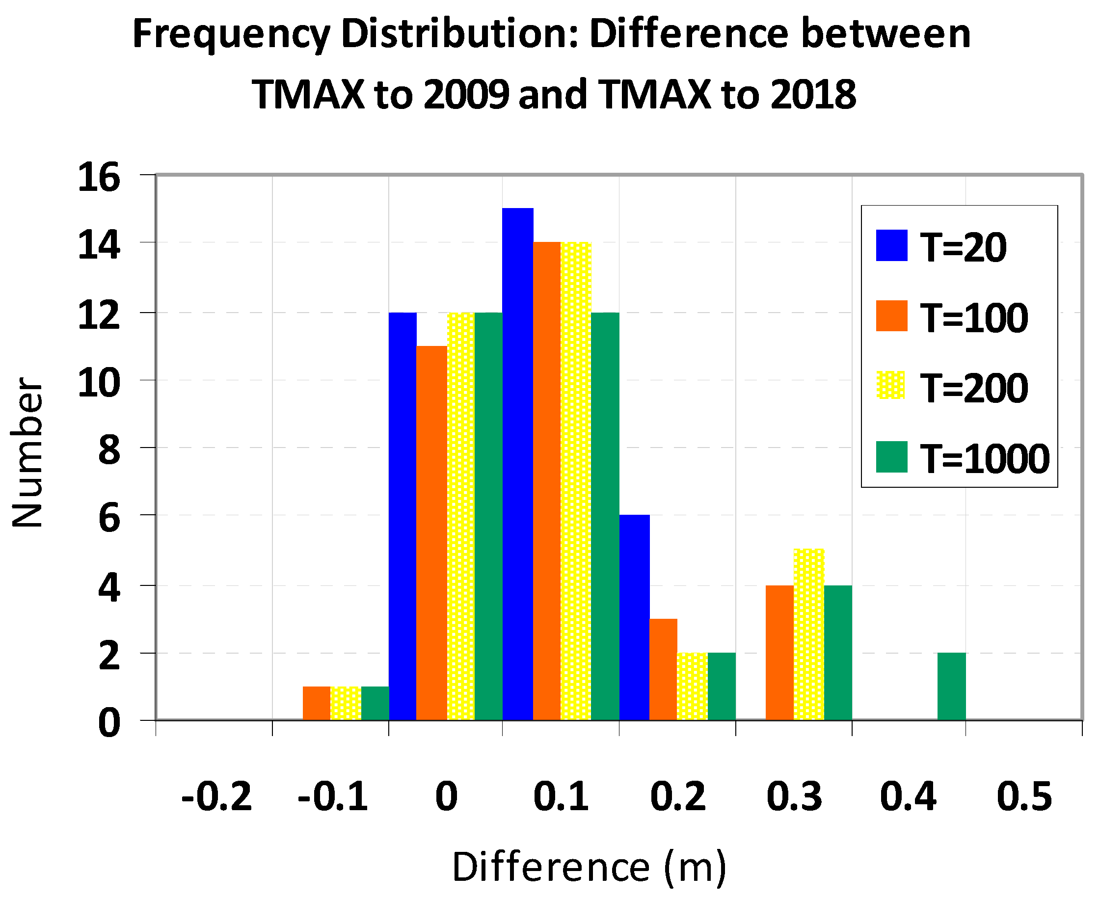
Figure 5.
Extreme Sea Level ODN (m) for a 100-year return period at selected locations in the UK. Colour indicates the change between 2009 and 2018, red: increase, green: decrease.
Figure 5.
Extreme Sea Level ODN (m) for a 100-year return period at selected locations in the UK. Colour indicates the change between 2009 and 2018, red: increase, green: decrease.
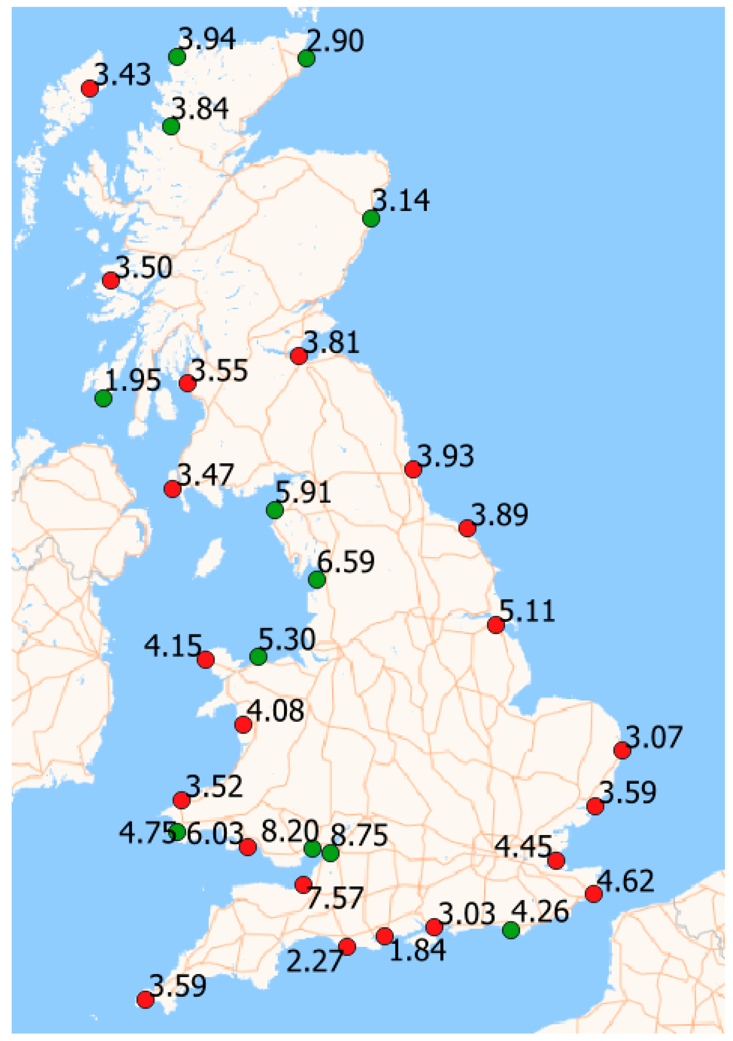
Table 1.
AMAX and TMAX methods. Quality of Fit of Regression Line.
| Variance of Mean σM (m) | Variance of Predicted σP (m) | |||||||
| Return Period (yr) | 20 | 100 | 200 | 1000 | 20 | 100 | 200 | 1000 |
| AMAX to 2009 | 0.09 | 0.10 | 0.11 | 0.13 | 0.39 | 0.39 | 0.39 | 0.40 |
| TMAX to 2009 | 0.02 | 0.03 | 0.03 | 0.03 | 0.24 | 0.24 | 0.24 | 0.24 |
| AMAX to 2018 | 0.08 | 0.09 | 0.09 | 0.11 | 0.41 | 0.41 | 0.41 | 0.41 |
| TMAX to 2018 | 0.02 | 0.02 | 0.02 | 0.03 | 0.26 | 0.26 | 0.26 | 0.26 |
Table 2.
Tabulated data for the TMAX method at Heysham, UK. Input duration span 19844 days, with valid data 17834 days i.e. 17232 tidal-days.
Table 2.
Tabulated data for the TMAX method at Heysham, UK. Input duration span 19844 days, with valid data 17834 days i.e. 17232 tidal-days.
| Rank | Date | Height(H0) (m) |
F(Ht>H0) * per tidal-day |
Return Period † years |
| 1 | 01/02/2002 13:45:00 | 11.36482 | 3.2E-05 | 87.20 |
| 2 | 10/02/1997 13:15:00 | 11.30877 | 9.1E-05 | 31.30 |
| 3 | 30/03/2006 11:45:00 | 11.25951 | 1.5E-04 | 19.07 |
| 4 | 02/01/2018 23:30:00 | 11.18499 | 2.1E-04 | 13.72 |
* Calculated using Eq. 5 with N=17232 samples. † Calculated using Eq. 6 with one tidal-day=1.034989 solar days.
Table 3.
AMAX and TMAX methods: Comparison with Batstone 2013.
| Mean Difference (m) | Standard Deviation (m) | |||||||
| Return Period (yr) | 20 | 100 | 200 | 1000 | 20 | 100 | 200 | 1000 |
| AMAX to 2009 | 0.00 | 0.03 | 0.04 | 0.06 | 0.11 | 0.16 | 0.19 | 0.27 |
| TMAX to 2009 | -0.01 | -0.03 | -0.04 | -0.07 | 0.09 | 0.13 | 0.15 | 0.22 |
| AMAX- to 2018 | 0.02 | 0.06 | 0.07 | 0.09 | 0.10 | 0.14 | 0.16 | 0.22 |
| TMAX to 2018 | 0.02 | 0.01 | 0.00 | -0.02 | 0.09 | 0.12 | 0.14 | 0.20 |
Table 4.
Rise in level averaged across 35 UK ports between TMAX (2009) and TMAX (2018).
| Return Period (yr) | 20 | 100 | 200 | 1000 |
| Mean Difference (m) | 0.031 | 0.041 | 0.044 | 0.055 |
| SD (m) | 0.066 | 0.088 | 0.096 | 0.121 |
| t score=M√N/SD | 2.706 | 2.678 | 2.653 | 2.623 |
| P (Significance=0.01) | 0.005 | 0.006 | 0.006 | 0.006 |
Disclaimer/Publisher’s Note: The statements, opinions and data contained in all publications are solely those of the individual author(s) and contributor(s) and not of MDPI and/or the editor(s). MDPI and/or the editor(s) disclaim responsibility for any injury to people or property resulting from any ideas, methods, instructions or products referred to in the content. |
© 2025 by the authors. Licensee MDPI, Basel, Switzerland. This article is an open access article distributed under the terms and conditions of the Creative Commons Attribution (CC BY) license (http://creativecommons.org/licenses/by/4.0/).
Copyright: This open access article is published under a Creative Commons CC BY 4.0 license, which permit the free download, distribution, and reuse, provided that the author and preprint are cited in any reuse.


