Submitted:
17 December 2025
Posted:
18 December 2025
You are already at the latest version
Abstract
Many quality characteristics of products or services are commonly evaluated on ordinal scales with a finite number of categories. A systematic analysis of categorical variables collected over time may be very useful for a profitable management strategy. In order to measure customer satisfaction or quality improvement in a process, two or more quality characteristics are often conjointly measured and summarized by suitable indexes. A common practice suggests evaluating a synthetic index by mapping each outcome of a multivariate ordinal variable into numbers. This procedure is not always legitimate from the measurement theory point of view. Recently the author read the paper “Synthesis maps for multivariate ordinal variables in manufacturing” and found in it many ideas about Control Charts for Services. We analyse them from a “scientific point of view” to compare the authors findings with ours. The analysis shows the “same (=equivalent)” results for the “linguistic control charts” and different results for the “numeric Control Charts”: the cause is that they do not use correctly the Theory. The Control Limits in the Shewhart CCs are based on the Normal Distribution (Central Limit Theorem, CLT) and are not valid for non-normal distributed data: consequently, the decisions about the “In Control” (IC) and “Out Of Control” (OOC) states of the process are wrong. The Control Limits of the CCs are wrongly computed, due to unsound knowledge of the fundamental concept of Confidence Interval. Minitab and other software e (e.g. JMP, SAS) use the “T Charts”, claimed to be a good method for dealing with “rare events”, but their computed Control Limits of the CCs are wrong. The same happens for the Confidence Limits of the parameters of the distribution involved in the papers (Weibull, Inverse Weibull, Gamma, Binomial, Maxwell).
Keywords:
linguistic variables
; fuzzy sets
; control charts
; exponential distribution
; T charts
; minitab
; JMP
; reliability integral theory
1. Introduction
Many quality characteristics of products or services are commonly evaluated on ordinal scales with a finite number of categories. A systematic analysis of categorical variables collected over time may be very useful for a profitable management strategy. In order to measure customer satisfaction or quality improvement in a process, two or more quality characteristics are often conjointly measured and summarized by suitable indexes. A common practice suggests evaluating a synthetic index by mapping each outcome of a multivariate ordinal variable into numbers. This procedure is not always legitimate from the measurement theory point of view [1,2,3,4,5,6,7].
Recently the author read the paper “Synthesis maps for multivariate ordinal variables in manufacturing” and found in it many ideas about Control Charts for Services. We analyse them from a “scientific point of view” by considering the following papers (Table 1); notice that around a central pin (author) there are seven members of the “Quality Engineering Group (QEG)” (all graduated CUM LAUDE), writing dubious ideas…
Notice the name “Qualitometro” (I, II and III), meaning “the Method for measuring Quality”.
The ideas in the table 1 papers have been taught for twenty-five years, at least.
Higher Education is seen many times as a Production System, and students are considered as its “Customers”. Books and magazines are suggested to students, attending “Quality Courses” at Universities. Some of them are good some are not so good. Students use papers from magazines for their teaching; some papers have good Quality some are not very good. Therefore it seems important to stand-back a bit and meditate, starting from a managerial point of view. In order to “measure” Quality (?) various bibliometric indices (e.g., h-index, s-index, Impact Points, RG-index, citations, …) have been devised, based on informetric models. Research Quality (?) in many universities is based on these indexes: if you are cited many times you are a better professor than if you are not! That’s the harsh reality… Let’s imagine that in one university there is a Quality Engineering Group (QEG, comprising seven lecturers, all graduated CUM LAUDE, and teaching "Quality matters"; they are also in the ResearchGate with high Impact Points and RG-index!). Until today, incompetent lecturers teach wrong ideas because they do not know Probability Theory. Statistic and Reliability Theory. Any rational person shall expect that those people will teach good ideas and will write “Quality papers on Quality matters”. Do those people act correctly or wrongly? We will see it. There is a must: professors must use the Scientific Approach when they teach, they must know what scientificness entails. Therefore it seems important to stand-back a bit and meditate, starting from a managerial point of view. The author cannot solve this huge problem: the Universities Management MUST solve it; the author can only mention very few cases of incompetent teaching: the Bass model [9] (invented by Bass in 1969; Bass himself made errors in the first time), and later, many professors copied, with irrational attitude, his ideas and diffused them to much more many students, all over the world. The same is for inventory management, for six sigma, for the fuzzy theory and for linguistic variables [1-7 and Table 1] applied to Quality. Notice that Zadeh [7] was dealing with “System Theory” before embracing fuzzy theory and for linguistic variables: this is very important in this paper! Many Journals provided wrong papers on Control Charts [8].
The basic theories needed to understand are Probability, Statistics, Reliability and Mathematics: nothing more is necessary [10,11,12,13,14,15,16,17,18,19,20,21,22,23,24,25,26,27,28,29,30,31,32,33,34,35,36,37,38,39,40,41,42,43,44,45,46,47,48,49,50].
Quality is essential for any product/service. The measurement of Quality (of product and services) is important if we want to improve and more important if we want to prevent problems. According to Quality Management Principle # 6: “Evidence-based decision making” all Companies (and their managers, people, workers, …) need to make their decisions using data and Good Methods (Quality Methods).
If data are available, scientific statistical methods are the foundation stone for good data analysis. The problem of "measurement" of Quality and of “quality characteristics” is very important; the use of "non-numeric" scales, linguistic variables and fuzzy logic are strongly suggested (by QEG) for "Quality evaluation", in order to avoid two problems
- "… encoding a discrete verbal scale into numerical form … introduces properties that were not present in the original linguistic scale … eliminates the meaning of the collected data … Scalarisation, introducing in the scale … some “metrological properties” … may determine a “distortion” effect on information meaning. … with intuitable consequences."
- "… the analyst of the problem does directly influence the acceptance of results. Consequently, by attributing numbers to verbal information we move away from the original logic of the evaluator…. Proper scales for this purpose are linguistic scales ... because the concept of distance is not defined."
According to Yager (1981) ["A new methodology for ordinal multiobjective decision based on fuzzy sets"] "… forcing the decision maker to supply information with greater precision than he is capable of providing. This may lead to incorrect answers …"; therefore, using linguistic scales and fuzzy logic one avoids the "tyranny of numbers".
Yager (1981) invented a method capable of dealing with non-numeric data. The analysis of the non-numeric data is justified (by Yager) via the use of "fuzzy logic".
Absolutely aware of Shewhart’s [27,28] and Deming’s [14,15] teaching "Without theory, experience has no meaning." and of the validity of the Scientific Approach, devised by Galileo Galilei [51,52], F. Galetto with this paper will analyse the findings of "Yager (fuzzy) Method" and compare them with a completely numeric method, based on Lattice Theory, with no "fuzzy concept".
Therefore, one can get a better understanding of what he can expect from a scientific application of fuzzy models to "Quality Evaluation".
We will consider the three types of “Qualitometro (I, II, III)” (Table 1) to become aware of the fakeness of the involved methods.
2. Materials and Methods
2.1. The Qualitometro I (Q I)
We first consider various statements of the QI authors. Their “Key Words” (the underline is due to FG): service quality; Service quality measurement; On-Line service quality control; Customer satisfaction”.
Notice that “customer satisfaction” è very different from da “Customer’s needs satisfaction”.
|
“Services and their quality are now the core of many investigative studies of managers and researchers. Many stimulating ideas and conceptual models have been proposed in such a way as to describe the mechanisms at the basis of delivered and received service. Developing this knowledge, there is now a strong need for proper service quality evaluation tools…. A great effort was made to specify and classify differences between the process characterizing a product and a service. Services are different in their intangibility, their limited standardization, and their contextual links, in place and time, between service production and delivery (impossibility to store), implying, usually, customer personal involvement. Finally, it is their heterogeneity resulting from the human factor that makes the service strongly affected by the conditions and the environment where it is delivered”. … “The central difference between products and services is the greater difficulty for the latter to ‘quantify’ them. This does not imply that for products, considered during their whole life cycle (not only in the product step), there is a simple solution for the analogous problem of global quality quantification”. ... “It is not easy for most services to define the qualitative elements to ‘observe’ which measurements are to be done and, no less, which test and checks to perform to control them”. “Many studies made efforts to realize how the customer perceives and evaluates the quality of received service, but to the problem’s complexity, the results represent only a promising beginning. Here, we offer a contribution to the growing discussion, suggesting an evaluation and on-line control of the gap between expected and perceived quality. In this context, on-line means evaluation during service delivery, remembering a term from control theory. “The main innovations of this method are the operative procedures for data collection and data elaboration”. “It is now common opinion among service operators that quality operators that quality comes from a stimulus of continuous comparison between expectations and perceptions. According to this criterion, Gronroos prepared a model founded on the assumption that the customer compares expected and the received service when evaluating quality… Some theoretical and empirical studies are offered as useful guidelines for service quality evaluation, control, and design”. “Suggestions by researchers found their base and consistency in some conceptual models for delivering service processes. Among them, the most famous and well know is that proposed by Parasuraman et al. If conceptual models are able to interpret service delivery steps on one hand to be used operatively on the other, they need to contain the values of the variables and parameters invoked, the evaluation of which is often other than immediate. To solve this problem, proper inquiry tools (questionnaires typically) able to collect customer evaluations are employed. The literature offers many tools to evaluate service quality. SERVQUAL and SERVPERF are two of the most well know and often used examples in the applications. Common feature of these methods are as followings: using questionnaires; the acknowledgement of the multidimensionality of quality (quality can be expressed as a set of attributes); considering expected and perceived quality or the latter only; ‘numerical’ interpretation of data collected in the questionnaires. The problem of the quantification service quality is solved by first stating the following: attribute affecting service delivery and their relative importance for the customer; objective and/or subjective measurable elements; ‘measuring systems’ adequate to evaluate attributes and variables; a proper model to define the link between variables and delivery process; procedures needed to monitor service delivery continuously; reference standards. People, mostly because of the diversity of each individual ‘reference system’ influence service evaluations substantially. |
Excerpt 1. Statements from “On-line service quality control: The ‘Qualitometro’ method”.
Notice “comparison between expectations and perceptions“ and “SERVQUAL and SERVPERF”.
See in the Figure 1 the way of collecting data. Notice the “linguistic” variables and their “indexes”…
|
“Nowadays, most of the questionnaires used to collect information on service quality use a point evaluation scale (1 to 7 or 1 to according to different versions) associated with adjectives to qualify a particular position. During data elaboration, scales are converted into numerical interval scale, and symbols are interpreted as numbers. Using these numbers, the statistical elaboration is then performed… …This conversion results in moving from an ordinal interval scale to a cardinal one”. “The scalarization of collected data presents two main problems: the first is in introducing through coding an arbitrary metric, resulting in a wrong interpretation of gathered data; the second is a hidden assumption for an identical scale interpretation by any interviewed individual and rigidity of this scale in time, especially for periodic service users. Scalarizationmay generate a ‘distortion’ effect, modifying the collected data partially or completely. A critical aspect of the question is that, usually, the entity of introduced distortions is not clear nor is the distance from the real value of the information given by customer”. “The Qualitometro method was created in order to evaluate and check on-line service quality”. |
Excerpt 2. Statements from “On-line service quality control: The ‘Qualitometro’ method”.
Two questionnaires are provided to the customers: the 1st before the service is provided, to collect information about the “expected quality” (the vector) Qe, the 2nd after the service delivery, to collect information about the “perceived quality” (the vector) Qp.
|
“The analysis of information collected on one scale and elaborated on another one, with different properties, causes some interpretation problems”. “During data elaboration, scales are converted into numerical interval scales, and symbols are interpreted as numbers. Using these numbers, the statistical elaboration is then performed. Thus, for example, if the ends of a seven-point scales are the statements strongly disagree and strongly agree and we associate to these the numerical symbols 1 and 7 and symbols from 2 to 6 to the intermediate statements, we have carried out a conversion results in moving from an ordinal interval scale to a cardinal one” . “The scalarization of collected data presents two main problems: the first is in introducing through coding an arbitrary metric, resulting in a wrong interpretation of gathered data; the second is a hidden assumption for an identical scale interpretation by any interviewed individual and rigidity of this scale in time, especially for periodic service users. Scalarizationmay generate a ‘distortion’ effect, modifying the collected data partially or completely. A critical aspect of the question is that, usually, the entity of introduced distortions is not clear nor is the distance from the real value of the information given by customer”. “In other words, the original information, ‘arbitrary’ enriched or directed to simpler aggregation and elaboration, may be highly modified if compared with the one really expressed by customers, with intuitable consequences”. “Qualitometro allows two possibilities for data elaboration: |
|
Excerpt 3. Statements from “On-line service quality control: The ‘Qualitometro’ method”
From the data (before and after the service delivery) the two “global qualities” qi, and qp are “computed”: if qp < qe the “service provided” is considered as “defective”; counting the numbers of defectives, the defectiveness p is computed (number of occurrences of the “negative event” to the total number of services provided). After that the “p Chart” is used with the related Control Limits, LCL and UCL [26,27].
Let’s consider the figure 1, where we see that the (vector) “expected quality” Qe=[2,4,4,5,5,3,2,4] with importances W=[3,1,3,4,5,4,1,3]; after the service delivery we have the vector “perceived quality” Qp=[4,5,4,5,4,4,1,5]; the two vectors have to be compared to “measure” if qp < qe. Using ELECTRE II the authors find p1=1 (the service is defective for the delivery of the 1st customer, with his importances W and vectors Qe and Qp). Doing the same for the other K customers the authors compute and from that LCL and UCL.
We can conclude, as we will see again in the following sections, that the scalarisation provides the same decisions as the linguistic variables!
2.2. The Qualitometro II (Q II)
The authors of “Service qualimetrics: the qualitometro II method” go on repeating:
| “Although numerization simplifies data elaboration for analysts, it eliminates the meaning of the collected data by the logic of evaluators/experts that delivered them. Scalarirization, introducing in the scale used to gather information some metrical properties higher than those really owned when supplied by the customer/evaluator, may then determine a distortion effect on information meaning. The critical side of the problem is that usually distortion is introduced and the shifts between arbitrary interpretation and customer opinion are not known ”. |
Excerpt 4. Statements from “Service qualimetrics: the qualitometro II method”
To understand F. Galetto findings let’s see other ideas of the QEG [in the above paper]; see a new Excerpt from the paper "On line Service Quality Control: the Qualitometro Method", Quality Engineering.
| «Another delicate question is the numerical coding for judgements expressed on interview questionnaires. … During data elaboration, scales are converted into numerical interval scales, and symbols are interpreted as numbers. … The scalarization of collected data presents two main problems. The first is in introducing through coding an arbitrary metric, resulting in a wrong interpretation of gathered data; the second is a hidden assumption for an identical scale "interpretation" by any interviewed individual and a rigidity of this scale in time, especially for periodic service users. Scalarization may generate "distortion" effect, modifying the collected data partially or completely. … In other words, the original information, "arbitrarily" enriched or directed to simpler aggregation and elaboration, may be highly modified if compared with the one really expressed by customers, with intuitable consequences.» |
Excerpt 5. Statements from “Service qualimetrics: the qualitometro II method”
Let’s see another Excerpt
| «Ordered linguistic scales mainly differ from numeric or ratio scales because the concept of distance is not defined. The ordering is the main property attributed to such scales. For example, on a production line for fine liqueurs, a visual control of the corking and closing process might have the following possibilities: (a) 'reject', (b) 'poor quality', (c) 'medium quality', (d) 'good quality', (e) 'excellent quality'. The monitoring of production, using sampling control technique, is aimed at recognizing and, possibly, correcting … out-of-control conditions. In order to do this the five classifications listed above could be attributed to some numerical values, leading to the construction, for example, of standard X-R charts. Although the numerical conversion of the verbal information simplifies subsequent analysis, it also gives rise to two problems. The first is concerned with the validity of encoding a discrete verbal scale into a numerical form. This approach introduces properties that were not present in the original linguistic scale (for example, is it legitimate to assume that the difference between the 'reject' state and the 'poor quality' state is the same as that between the 'medium' and 'high quality'?) [notice: 'high quality' does not exist (in the "possibilities"!] Moreover, unlike scales used for physical measurements, ordered linguistic scales do not have either metrological reference standard or a measurement unit (QEG). The second problem is related to the absence of consistent criteria for the selection of the type of numerical conversion. It is obvious that changing the type of numerical encoding may determine a change in the obtained results. Introducing arbitrary weight for quality categories may condition substantially the way of interpreting the process evolution. For example, if we assign to each quality level for a five-level scale, the series of numbers: 1, 2, 3, 4, 5, or the series: -9, -3, 0, 3, 9, we obtain two different results. In this sense the analyst of the problem does directly influence the acceptance of results. Consequently, by attributing numbers to verbal information we might effectively [sic] move away from the original logic of the evaluator. In this way any conclusion drawn from the analysis on 'equivalent' numerical data could be partially or wholly distorted. … The fuzzy operator that is used in the paper allows for this flexibility in the decision logic.» |
Excerpt 6. Statements from "Control Charts for linguistic variables: a method based on the use of linguistic quantifiers"
The three “tenors” (authors in the Table 1) repeat:
|
“For data elaboration, Qualitometro I allows two possibilities: Statistical data analysis according to the traditional approach (after data numerization), Central tendency and dispersion estimation without any numerical coding of collected information. Qualitometro I develops also a consistency test for gathered information. We now present and discuss a new proposal for data processing that enhances elaboration capabilities of Qualitometro I. This new procedure, named Qualitometro II, is able to manage information given by customers on linguistic scales, without any arbitrary and artificial conversion of collected data”. “Collecting and treating data by means of the Qualitometro II eases this process, providing a method for performing elaboration closer to the customers’ fuzzy thoughts” |
Excerpt 7. Statements from “Service qualimetrics: the qualitometro II method”
Notice: “… elaboration closer to the customers’ fuzzy thoughts“.
Following [1,2,3,4,5,6], the authors write:
|
“The method proposed may be classified among the ME–MCDM (multiexpert–multiple criteria decision making) techniques”. “It is able to handle information expressed on linguistic scales without any artificial numeric scalarization. The use of linguistic scales introduces many constraints in the data elaboration process. As an example, we consider the calculation of the distance between two scale elements: this operation is fully defined on a numeric scale (with ratio or interval properties), but is not on an ordered linguistic scale. We assume the hypothesis of homogeneous interpretation of linguistic terms by each expert. In this manner, it is possible to ‘aggregate’ information coming from different evaluators”. “The authors propose interpreting any criterion as a fuzzy subset on the set of alternatives ai to be selected. If gj is the jth criterion (j=1, …, n), then the membership degree of an alternative ai to gj shows the degree to which the same alternative satisfies the criterion”. “The second idea given in the Bellman and Zadeh approach to how a DM (Decision Maker) aggregates evaluations expressed for each evaluation criterion”. “Particularly, they suggest the following relationship as a logical aggregating operation: where is the symbol of the logic operator “and” according to fuzzy logic interpretation”. For , (A is the set of alternatives) the decision function then becomes ... and following Yager (1993) (introducing the Importances) . “According to this model, global evaluation indicators for expected and perceived qualities given by the kth evaluator (k=1, …, s) becomes respectively: are the evaluations expressed by the kth evaluator on the jth criterion about expected (Qe) and perceived quality (Qp) respectively; the terms are the negations of the importances assigned to each evaluation criterion”. “It is worthwhile to emphasize that the provided aggregation does not perform any arbitrary scalarization of information given by evaluators on linguistic scales”. |
Excerpt 8. Statements from “Service qualimetrics: the qualitometro II method”
Notice and remember the last statement in the Excerpt 8! We will see it is false!
2.3. The “Fuzzy Sets” and the “Lattice Theory” for the Qualitometro II (Q II)
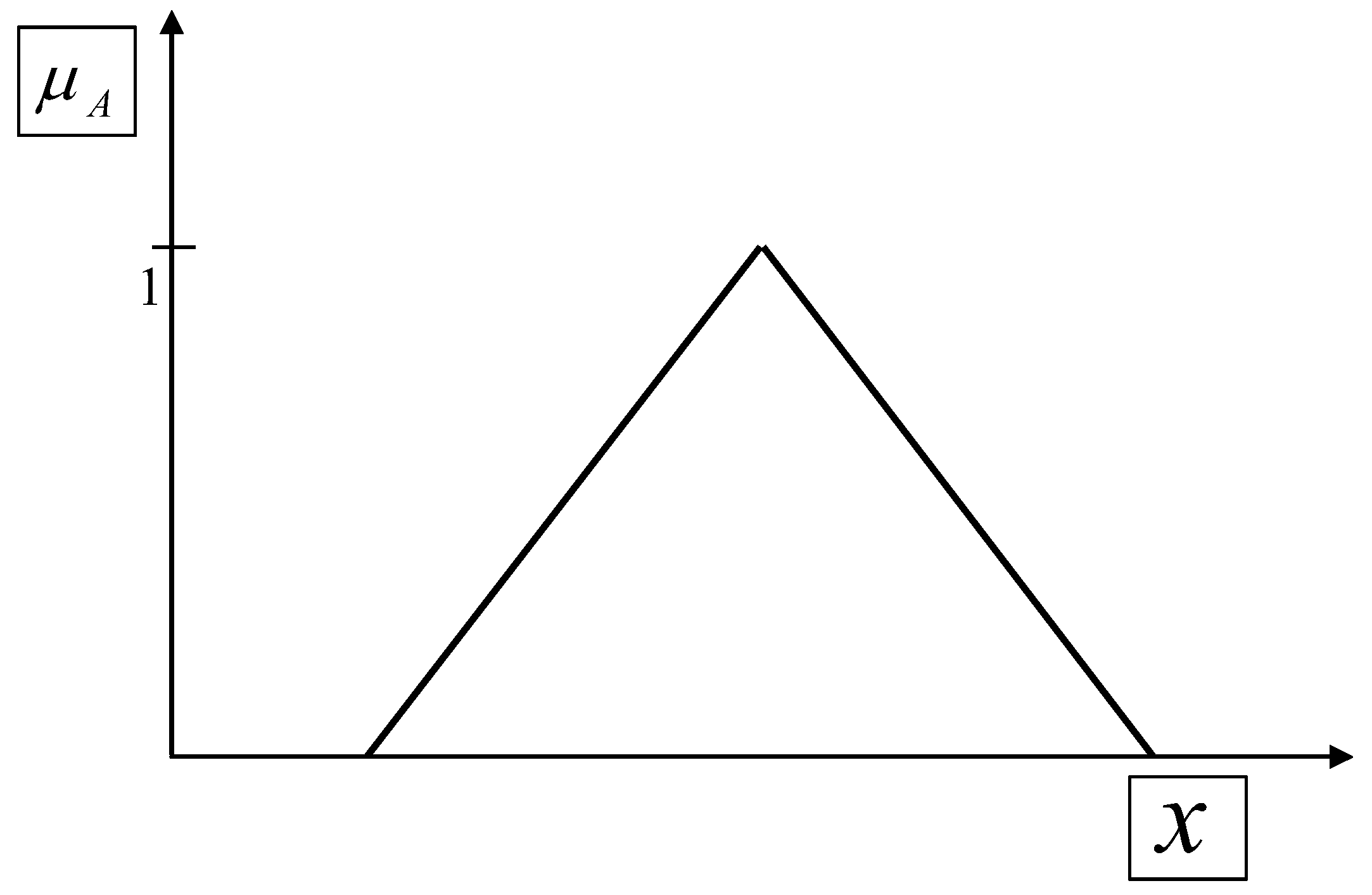
Figure 2.
Grade Of Membership (GOM) of the “fuzzy set” A (x∈A); x “base variable”
If the Qualitometro uses the “Fuzzy Theory” [1,2,3,4,5,6], then it must have the GOM as figure 3 (for example).
Figure 3.
A possible GOM for the Qualitometro
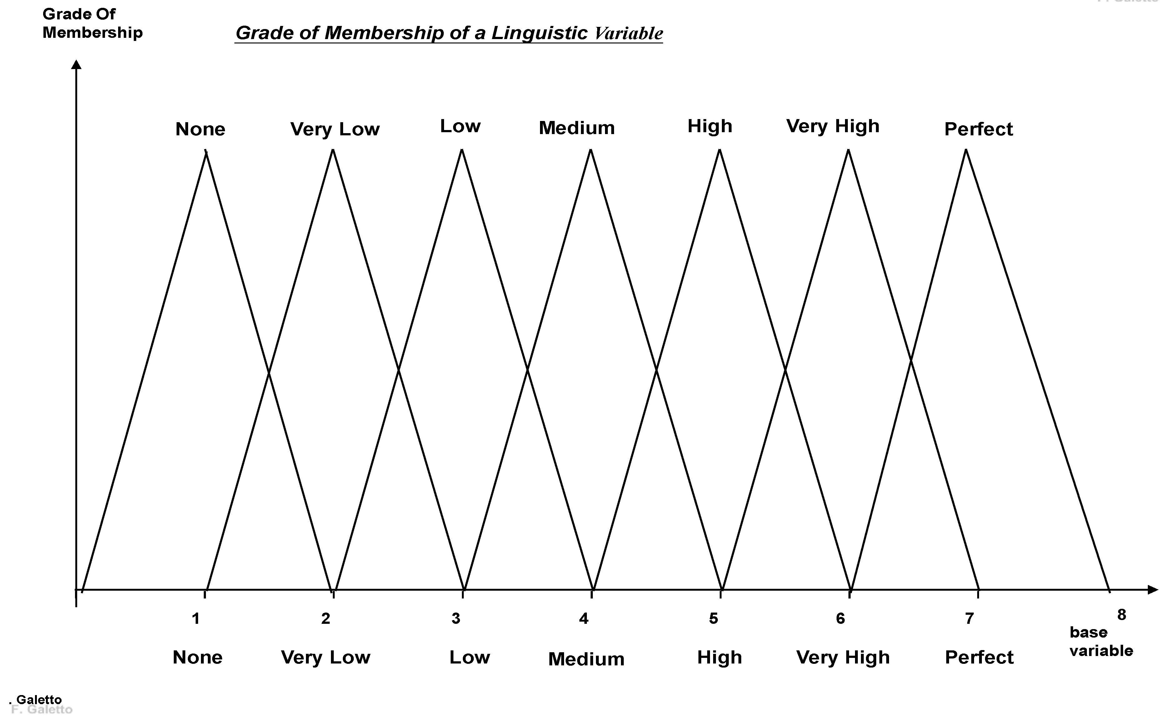
The important concept related to the “Fuzzy Theory” [1,2,3,4,5,6] is that a “fuzzy set” A is a couple of two “mathematical things” [A, μA(x); x∈A, x “base variable”], where A is a “usual set” and μA(x) [symbolised by GOM] is a “usual mathematical function” (e.g. triangular as in the figure 2; it can be any type of function). NO GOM then NO Fuzzy [1,2,3,4,5,6].
Looking at all the Qualitometro papers you never find the GOM.
Actually, the Qualitometro authors pride themselves by writing
| "The main difference of this method [Qualitometro!], with respect to others inspired by fuzzy logic, is that it does not require explicit information on the membership function"! |
Excerpt 9. Statements from “…..the qualitometro method”
No reader can find WHERE the fuzzy sets and grades of membership [membership function] are used, in the Qualitometro, while he finds the fuzzy sets and grades of membership [membership function] are used, in the paper of Yager, R. (1981) "New methodology for ordinal decision based on fuzzy sets", Decision Sciences, 12, 589-600, in the example of cars Chevrolet, Buick, Toyota; he can find HOW the membership grades [GOM] are drawn from the proposed linguistic scale, in the Qualitometro and in the paper Yager, R. (1981), in the example of cars Chevrolet, Buick, Toyota.
As stated before, absolutely aware of Shewhart’s, Deming’s and Galilei teaching and of the validity of the Scientific Approach, F. Galetto with this paper will show various numeric methods, based on Lattice Theory and other mathematical ideas, with no "fuzzy concept". Therefore, one can get a better understanding of what he can expect from a scientific application of fuzzy models to "Quality Evaluation".
Let’s start with the Partially Ordered Sets (PAS): a relation ≼ on a set X is called a partial order on X if and only if for every x, y, z ∈X the following 3 conditions are satisfied: 1. x≼x (reflexive) 2. x≼y and y≼x ⇒x=y (antisymmetric) 3. x≼y and y ≼z ⇒ x≼z(transitive) The inverse relation of≼, denoted by≽, is also a partial order on X. The dual of a partially ordered set X is that partially ordered set X* defined by the inverse partial order relation on the same elements. We have (X*)*=X: every set is the dual of its dual.
Notice that (figures 1, 3 of the Qualitometro) the seven-point scales define two PAS both for (Service) Importances and Evaluations.
A lattice L is an algebra with two binary operations [symbolised by ∩ and ∪ satisfying for all elements a, b, c in L the following axioms (Dedekind, in the 1890’s)

Table 2.
The Axioms of a Lattice
| Sequence | Axioms A | Axioms B |
| I | To every ordered pair (a, b) of elements a, b is assigned a unique element a∩b of L. |
To every ordered pair (a, b) of elements a, b is assigned a unique element a∪b of L. |
| II | (Commutative property of ∩) a∩b = b∩a | (Commutative property of ∪) a∪b = b∪a |
| III | (Associative property of ∩) a∩(b∩c) = (a∩b)∩c | (Associative property of ∪) a∪ (b∪c) = (a∪b) ∪c |
| IV | (Absorption property of ∩) a∩(a∪b) = a | (Absorption property of ∪) a∪(a∩b) = a |
Notice that the Axioms B are the “duals” of the Axioms A and vice versa: it suffices to exchange ∪ by ∩.
If we define a relation R between two elements of a lattice by aRb ⇔ a∩b = a, we can derive that aRb ⇔ a∪b = b; therefore, a lattice is a partially ordered set, with a≤b meaning a∩b = a and a∪b = b. If we define a∩b as the h.c.f. (a, b) and a∪b as the l.c.m. (a, b), we see that a≤b means h.c.f. (a, b)=a, that this a|b [a divides b]; with this definition all the sixteen factors of the natural number 216 are ordered. If we define a∩b as the min(a,b) and a∪b as the max(a,b), we see that a≤b means min(a,b)=a, that this a is equal or lower than b; with this definition all sets of natural numbers can be ordered. It easily proved that a lattice is always a partially ordered set, with a≤b meaning a∩b = a and a∪b = b. Therefore, lattice theory is perfectly able of dealing the linguistic variables, by transforming them into numbers! Logic says that!
A very important point is that in every lattice L exist two values the GLB (greatest lower bound) GLB and the LUB (least upper bound).
A very important Theorem states that “exist isomorphic lattices”).
Isomorphic lattices are lattices that are structurally identical, meaning they have the same properties and operations. This is defined by a bijective (one-to-one and onto) function between them that preserves both the GLB and LUB (least upper bound) operations. In essence, one is a perfect map or structural replica of the other. Lattice isomorphism is defined as an order isomorphism between two lattices, indicating that they are structurally identical in terms of their order.
Key characteristics of isomorphic lattices
- Structural identity: Isomorphic lattices are indistinguishable from a structural point of view. One is essentially a copy of the other, just with different labels for its elements.
- Bijective map: An isomorphism is a bijective function, meaning every element in the first lattice corresponds to exactly one element in the second, and vice versa.
- Preservation of operations: The most crucial property is that the function preserves the lattice operations. For any two elements a and in the first lattice (), and their corresponding elements in the second lattice () denoted as and , we have:
These ideas are fundamental for our critic to Qualitometro.
2.4. Various Few Cases of “Scalarisation” for the Qualitometro (Q I and Q II)
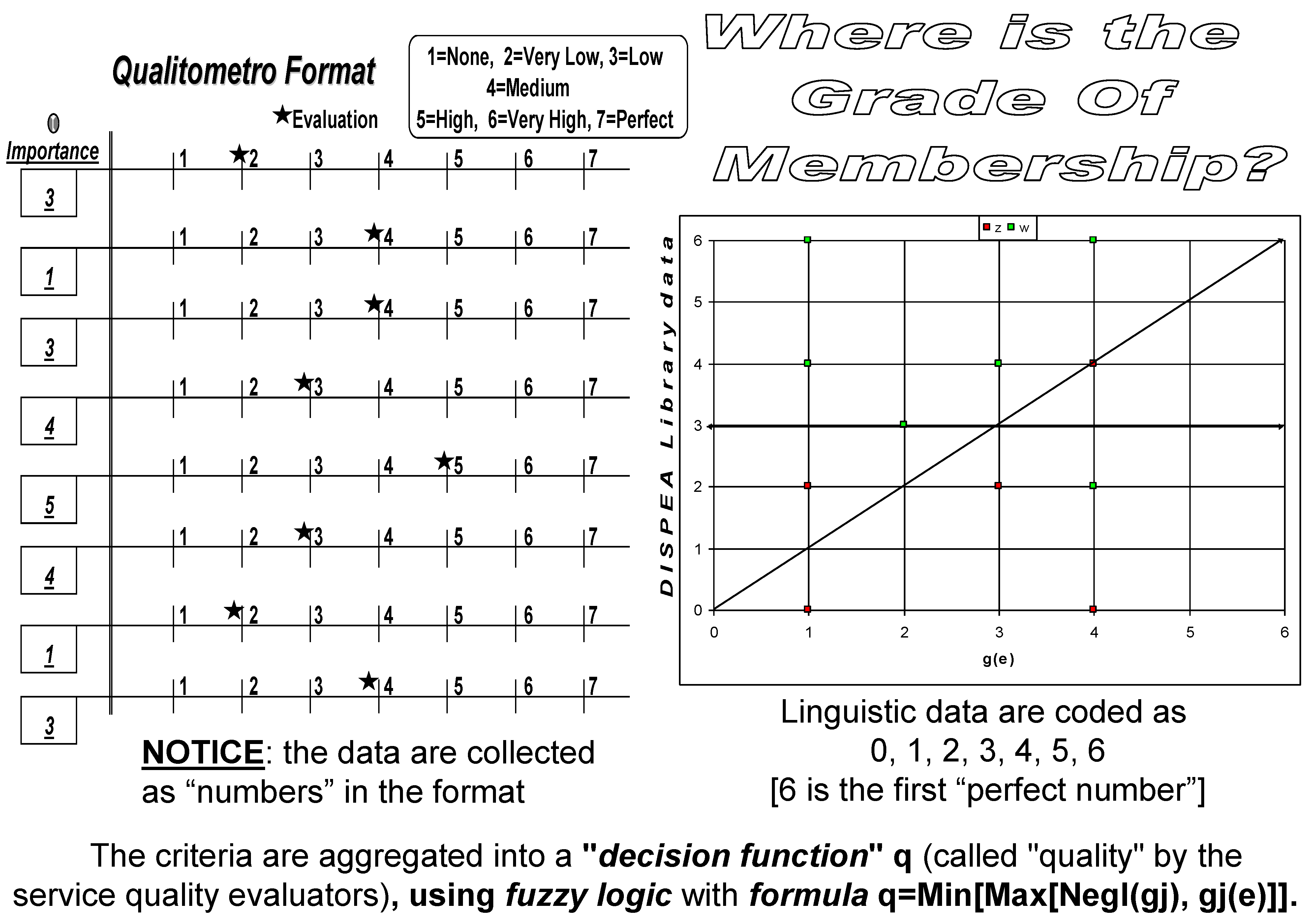
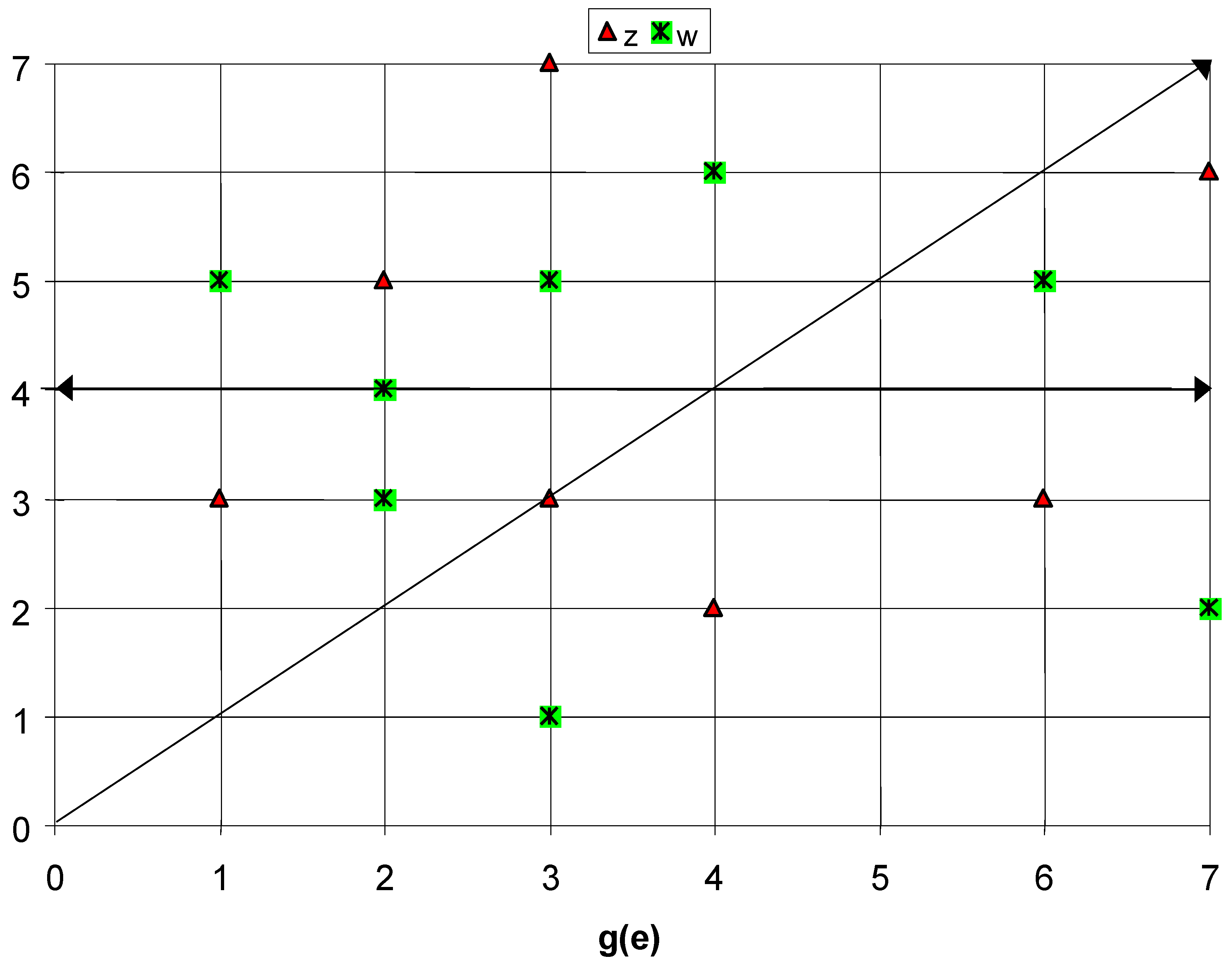
NOW, we purposely make what is forbidden and made our worst use of: numerical scales, scalarization, arbitrary and artificial conversion of linguistic collected data, distance and metric concepts, non-fuzzy logic and operators, … and we found the shocking result: (see figure 4, right side):
we get the same quality evaluation:all those "fuzzy" requirements are not essential.
Since we are fully aware of the validity of the scientific approach, let's apply the ideas given in the introduction: to understand the real validity of Yager Fuzzy Method, we purposely make a scalarisation, using the scale 0, 1, 2, 3, 4, 5, 6 [integer numbers, which form a chain (a very simple lattice)], and using a one-to-one mapping from the linguistic scale [None, Very Low, Low, Medium, High, Very High, Perfect] into the integer numerical scale [0, 1, 2, 3, 4, 5, 6 (a chain)], and vice versa, both for the evaluation "gj(e)" to jth criterion (jth "quality characteristic") and for the importance I(gj) of each evaluation criterion.
Notice: we used the "first perfect number" 6 [Euclid] for the linguistic Perfect, and the "first number" 0 [Peano] for the linguistic None; the number 0 is the least element of the chain, called "zero element" (in Algebra), and the "first perfect number" 6 is the greatest element of the chain, called "one element" (in Algebra), of the set [0, 1, 2, 3, 4, 5, 6]. It is very interesting that any number of the scale is a suitable power of the number 3 "the generator" [for the linguistic Medium] modulo 7 [written shortly mod7]; therefore "6=33 modulo 7" Ideas like these were invented thousands of years ago by Euclid. The subset [1,2,3,4,5,6] is a finite Abelian group: any element a has one inverse a-1; the product of two elements is an element of the group (closure); the multiplication is associative; there exists the identity [or one] element. Any integer number is congruent to an element of the set [0, 1, 2, 3, 4, 5, 6]: "congruent to" is an equivalent relation (reflexive, symmetric, transitive); there are 7 equivalence classes; equivalence is preserved under addition, subtraction and multiplication. All these properties are well known in Algebra.
Figure 4.
Points from the Qualitometro (for collecting data left) and NUMERIC Method (right, FG). There is no GOM (Qualitometro) and the Cartesian Plane π (on the right)
Figure 4.
Points from the Qualitometro (for collecting data left) and NUMERIC Method (right, FG). There is no GOM (Qualitometro) and the Cartesian Plane π (on the right)
We used Logic and Algebra [as a μαθητης]; let's now use Geometry and Calculus [as a μαθητης].
Let's consider a plane π, with Cartesian co-ordinates, ["Cartesian product" of the two chains (lattices L1 and L2) for the importance and for the evaluation is a lattice again (L)] the couple (x, y) define a vector OP; the Euclidean norm ρ provides the length of the vector (the distance of the point P from the origin O). Therefore the "complete" information provided by an evaluator is given by 8 vectors [8 "quality characteristics"], defined by the length and the direction of 8 segments OP1, OP2, …, OP8. We consider then another one-to-one mapping (involution) between the plane π (the lattice L, points named z in fig. 4) and the plane π' (the lattice L', points named z in fig. 4) defined by the relationship (called "involution") x'=x, y'=33y-1 modulo 7; the 8 vectors OP1, OP2, …, OP8 are transformed into 8 vectors OP'1, OP'2, …, OP'8. For each vector we define the norm |OPi|=max(|xi|, |yi|) and obviously |OP'i|=max(|x'i|, |y'i|); the minimum norm vector is given by formula q'=Min [|OP'i|], which provides the aggregated "mapped" result of the Yager Fuzzy Method. Therefore, one gets the same decision both if uses the linguistic scale [N, VL, L, M, H, VH, P] and if uses the numerical scale [0, 1, 2, 3, 4, 5, 6], with the metric (norm) |OP'i|=max(|x'i|, |y'i|)!
Why DOES F.G. GET THE SAME Yager RESULT, using “numbers” and without using the “fuzzy theory”? [fig.5]
But there is a completely numeric (algebraic) way. For each "quality characteristics" we compute the number
wi =[((xi+33yi-1 mod7)+ASS(xi-(33yi-1 mod7))/14-INT(((xi+33yi-1 mod7)+ASS(xi-(33yi-1 mod7))/14))*7
and then min (wi) provides the number, that anti-transformed, gives the "Fuzzy Result"!
All that depends on the isomorphism existing (because we generated it) between the "LINGUISTIC Fuzzy Space" and the "NUMERIC (Algebraic) Space". The linguistic scale [N, VL, L, M, H, VH, P] and the integer numeric scale [0, 1, 2, 3, 4, 5, 6] are isomorphic; it is well known (in Algebra) that "An isomorphism between partially ordered sets is an equivalence relation (reflexive, symmetric, transitive)".
At this point, there should be no doubt, to any "Intellectually Honest" person, that the statement "Scalarisation, introducing in the scale … some "metrological properties" … may determine a "distortion" effect on information meaning … introducing through coding an arbitrary metric, resulting in a wrong interpretation of gathered data. … It is worthwhile to emphasize that the provided aggregation does not perform any arbitrary scalarization of information given by evaluators on linguistic scales. … Refusal of an arbitrary encoding of scale levels means that a method must be devised for introducing an average operator on a scale where the distance concept ("norm") is not defined …". are false. Scalarisation does not introduce "distortion". Logic says that. It is like if we, in the 2-dimensions geometry, we refused the 5th parallel axiom and we got the Euclidean geometry as well: a very wrong result.
One can think that the mapping (isomorphism) into the numerical scale [0, 1, 2, 3, 4, 5, 6] was only a lucky choice: there are infinite mappings, due to isomorphism (which is an equivalence relation) of any finite chains with the same number of elements; two of them are [1, 2.5, 4, 8.5, 17.5, 35.5, 71.5], [1, 3.5, 6, 13.5, 27.5, 57.5, 116.5]; {other two [1, 2, 3, 4, 5, or -9, -3, 0, 3, 9] were given by Franceschini et al. who did not realise that!}. Obviously, the involution is not defined by the relationship given before: in any case a suitable transformation exists and is not reported here.
We could stop here, mentioning only that there are other several proofs of the falseness of the statements related to the Yager (Linguistic) Fuzzy Method and to Qualitometro. No "fuzzy" concepts are EVER used! The interested reader shall contact F. Galetto.
Now suppose that a REFEREE (PR, Peer Reviewer) enters the game.
- IF the PR says "Galetto did not provide the proof of the falseness of Qualitometro and Yager methods" HE is wrong: F.G. used numbers, distance, and no GoM, and he found the "SAME"=EQUIVALENT results [see fig. 4, 5]
- IF the PR says "Galetto did not provide the right formulae" HE is wrong: F.G., up to now, gave two methods, one geometric, another algebraic (F.G. can provide more than 20; some are given later).
Is it not relevant and not interesting for Quality Education that the methods proposed by the members of "international scientific community" (table 1) and Yager [in the magazines Quality Engineering, International Journal Of Production Research, and Decision Sciences] claim wrong statements? All those papers were Peer Reviewed by members of "international scientific community". Do you think they did a good job?
The three "tenors" give the lie to their statements: fuzzy logic is useless.
F.G. EVER was ready to meet any of the authors cited in this paper, and explain them way they were (and are) wrong, IF they wanted (want) to understand: nobody EVER accepted TO LEARN, up to now.
F.G. does not know if any book authors ever wrote that they had made errors: F.G. did it. On pages 107, 108, 109 of his book "Qualità. Alcuni Metodi Statistici da Manager" ["Quality. Some Statistical Methods for Managers"] he shows one error he made, that was discovered by a student of him: the proposed method is a very good approximation in some cases, but can provide wrong decisions in other cases: therefore, it is not "scientific". He did not (as he does not) have any problem in showing his errors: any honest person must do that.
Figure 5.
Qualitometro (linguistic) versus NUMERIC Method (F. Galetto).
Again, on purpose, we do what is forbidden: we transform the linguistic "data", Fj e Ij, into numbers and make all the computations with the numbers: this should case wrong results! Each questionnaire collects 8 couples of values Fj and Ij; il " FF method " provides a unique value q (quality of the given service), which is a value of the linguistic scale, using the "fundamental" formula [like the one invented by Yager] q = Min[Max[NegIj, Fj]], originating from "fuzzy logic " [is that true??]; q is a type of linguistic mean.
Figure 6.
Electric circuit (Fibonacci sequence, NUMERIC Method, F. Galetto).
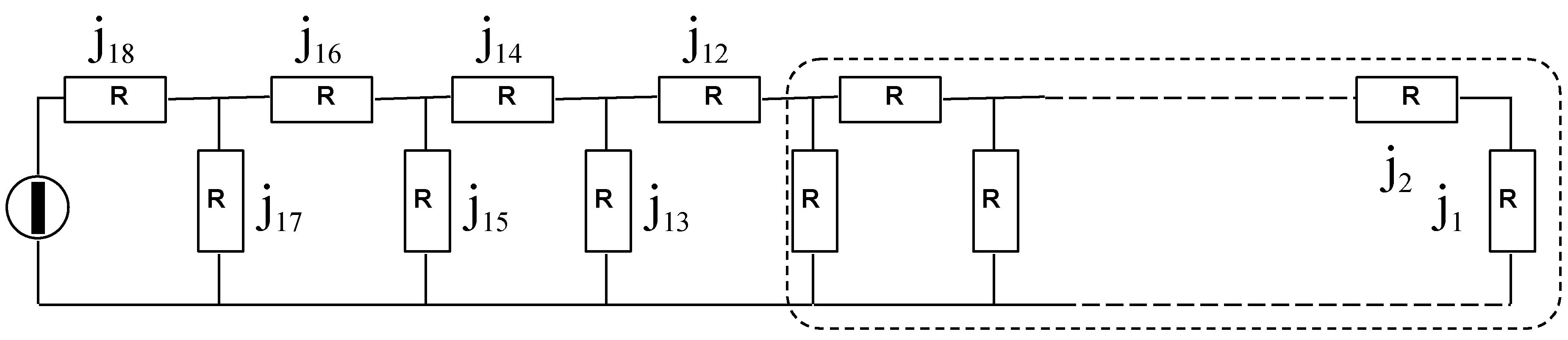
Let’s see a new numerical method. Consider an electric circuit consisting of resistors of resistance R and a battery (source of power supply) having a potential difference DV (e.m.f) across its terminals, made by several resistors as in the figure 6. We chose the resistance R and the e.m.f in a such a way that the current j1 is 1 nA. The various currents flowing are ji+1 = ji + ji-1, [relation like the one generating the Fibonacci series (Liber Abbaci, 1228)]: 1, 1, 3, 5, 8, 13, …, 144, …, 1597, 2584, …; the ratio of two successive numbers tends to the golden section "a=0,618034…" of a segment of length 1 m (known to all young students). For i→∞ we have j∞ = 1,618034…* ji.
We build ideally ("gedanken experiment", as done by Galilei and Einstein) a Black-Box with 8 “7-shot” knobs, to express "our evaluation Fj on the 8 characteristics of the service quality" and other 8 “7-shot” knobs for "our importance Ij on the 8 characteristics of the service quality". We measure the power delivered to each resistor:
- I)
- For evaluations, we associate the 1st of the “7-shot” s1 to the power [named x1] connected to the current j12, and so on till the last the “7-shot” s7 to the power [x7] connected to the current j18,
- II)
- For importances, we associate the 1st of the “7-shot” s1 to the power [named y1] connected to the current j18, and so on till the last the “7-shot” s7 to the power [y7] connected to the current j12.
The Black-Box computes the ratio xi/yi of the two powers: if the ratio xi/yi ≤ 1 then the value yi is stored in the ith memory (related to the ith characteristic), while if the ratio xi/yi > 1 the value xi is stored in the ith memory.
The display of the Black-Box at the end shows the integer number z, 1≤ z ≤ 7, where z is the sub-index of the current jz related to the minimum power stored: 1 for the current j12, 7 for the current j18. The "output" number, without using the fuzzy theory, is the "numeric" equivalent of the "FF method".
A new proof that we can use the numbers for Qualitometro.
If the "FF method" is sound, then it is sound using also the numbers: logic consequence!
Remember, as well, that the authors of the "FF method" pride themselves with the statements: "The main difference of this method, with respect to others inspired by fuzzy logic, is that it does not require explicit information on the shape of the membership function of the level of the linguistic scale." NO GoM, NO FUZZY!
All that should be enough. But we want to do our best to make errors: we use the distance concept, that the authors of the "FF method" state that does not exist: “... an arbitrary metric, … distance concept (“norm”) “,…“Scalarisation, … with intuitable consequences.” are nonsense.
Let’s consider the matrices in the Table 3; V is the payoff matrix of a game of two players betting in accordance with the vectors of the evaluations and the importances : the mean gain of the game (form game theory) is the dot product (scalar or inner product) ,.
V is the matrix build by 7 vectors SEPUF (System Expected Profit Until Failure) [F. Galetto 1975, 77, 86, 97] of a stand-by reparable system of 8 units with (constant) failure rate λ=1/ns and (constant) repair rate μ=1/ns, with a reward matrix R for each entrance in any state [F. Galetto 1975, 77, 86, 92, 97]. In such a way, performing myriads of prohibited operations (numbers, random variables, stochastic processes, games, metric spaces, …), one gets the “same result (=equivalent)” of the fuzzy formula of “FF method”. That means that the statement “Scalarisation, … with intuitable consequences.” Are scientific nonsense.
The reader could think the equivalent result (isomorphism) depends on the “numeric scalarisation 1, 2, 3, 4, 5, 6, 7”; actually, it is easy proved the contrary, by using different scalarisations and by repeating the reasoning.
The following method, the “turbine”, demonstrates geometrically another equivalent method, out of the many we can conceive. It does not need any computation, but only a pair of compasses.
Figure 7.
The turbine (Geometric-NUMERIC Method, F. Galetto)
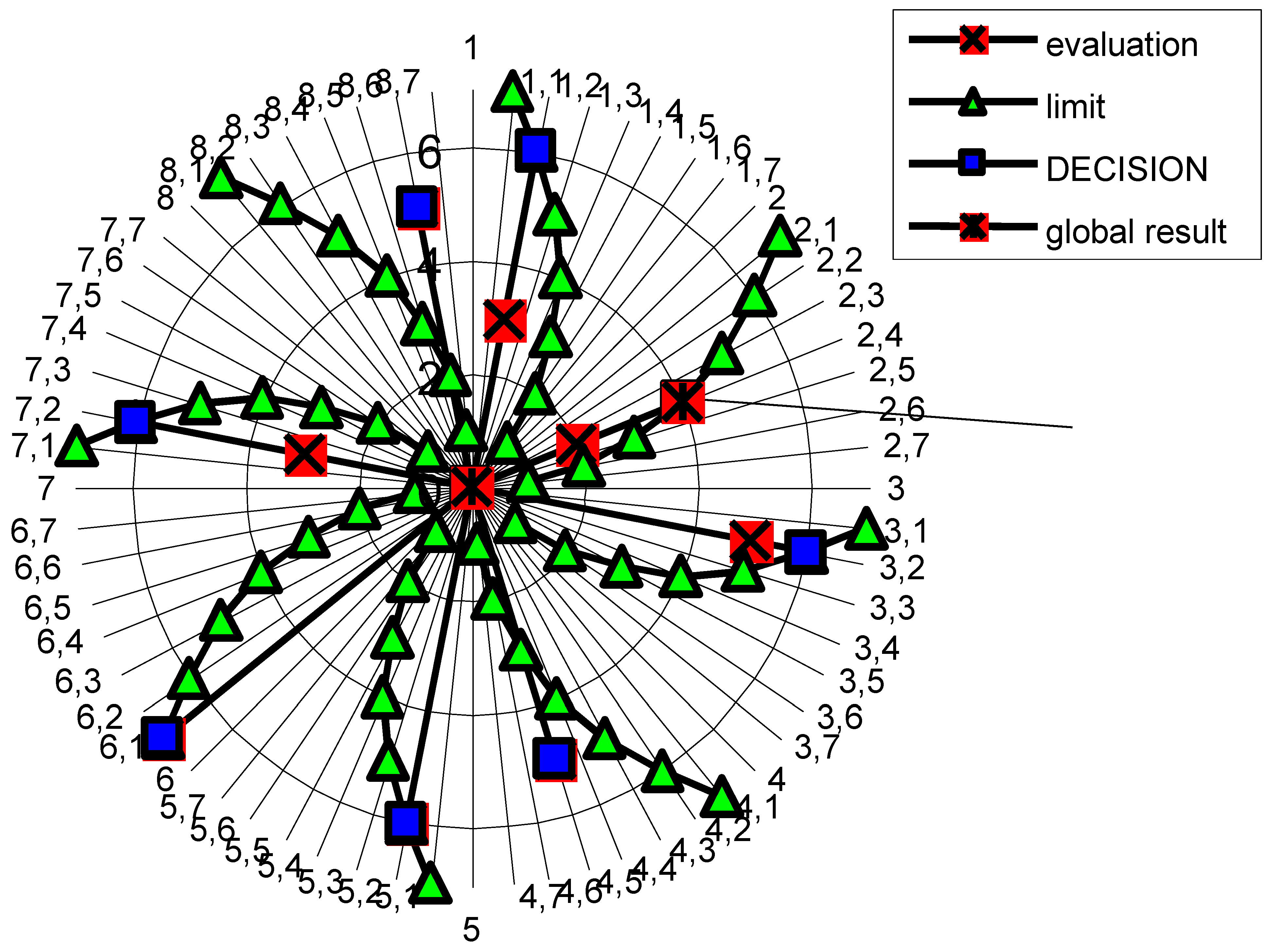
We first use the numbers 1, 2, 3, 4, 5, 6, 7, but the result is valid for other “metrices”. Let’s indicate with a decimal number j.y the importance y for the characteristic j (e.g. 3.5: characteristic 3 with importance 5) and with xj the evaluation for the characteristic j (e.g. 43: evaluation 4 for the characteristic 3). In a plane with polar coordinates, O be the origin and z the vertical axis from which we measure “clockwise” the angles. For each characteristic j we draw a radius vector OPj with length xj and “angle” connected to the importance j.y; so, we have 8 radius vectors OP1, OP2, …, OP8 (“metric” in the Euclidean plane) showing the collected in formation for the 8 characteristics. We put 8 marbles on the points Pj, and we make the turbine rotate: the centrifugal force sends the “internal” marbles against the turbine blades, while the “external” marbles maintain their position Pj; at the end of the process the marbles go to the “new” positions P'j; the marble with the minimum radius vector OP’j (i.e. the point nearest to the origin, provides the result “equivalent to the linguistic value of the fuzzy formula of the FF method”, as seen in the figure 7. We think that nobody can deny that we used “metric concepts”, forbidden by the Qualitometro authors.
The same information (in the figure 7) codified with a different metric [i.e. with the numbers 1, 2.5, 4, 8.5, 17.5, 35.5, 71.5] provides the “equivalent” aggregate quality; the same would happen even though we use a “new” codification [1, 3.5, 6, 13.5, 27.5, 57.5, 116.5]. Obviously, we need to define the function providing the distance: as usual, the minimum radius vector OP’j (i.e. the point nearest to the origin, provides the result “equivalent to the linguistic value of the fuzzy formula of the FF method”, as seen in the figure 7. Therefore, the statements of the Qualitometro authors "Scalarisation, introducing … “metrological properties” … arbitrary metric, resulting in a wrong interpretation of gathered data. …" and "It is important to emphasize that the control charts in this article are substantially different from the traditional X-R charts. We remind the reader that linguistic variables are defined on linguistic scale on which the distance concept and then a metric are not defined" are false.
We used before Logic and Algebra [as a μαθητης]; let's now use Calculus [as a μαθητης]: we use the Complex Numbers Method; the field of complex numbers is a complete numeric field (a Banach filed, as proved by Gauss), which does not have the “order property”: so, we cannot use the "fundamental" formula q = Min[Max[NegIj, Fj]], that they say originated [true??] by "fuzzy logic".
Let's consider the Complex Plane π, with Cartesian co-ordinates, y for the importance and x for the evaluation; the complex number zi=xi+jyi (4+j5 for the characteristic i=3) provides the complete information on the characteristic ith. The complete information on the 8 characteristics is given by the set of 8 complex numbers z1, z2, …, z8. It is well-known the complex numbers are shown in the plane π as vectors OP=z=x+jy; the modulus |z| is the length of the vector [Euclidean norm]; the ratio y/x is the tangent of the angle θ of the vector with x axis.
Consider the functional transformation ("involution" in Mathematics) w=8j+z* (z* conjugate complex of z); we get 8 complex numbers w1, w2, …, w8 "equivalent to the 8 couple of the "fuzzy" formula [gj(e), NegI(gj)]. The " aggregate result" provided by the "fuzzy" formula q= Min[Max[gj(e), NegI(gj)]] is the projection, on the nearest axis, of the vector of minimum length [norm]: if w0 is the complex number with r=Min(|wi|) and θ0 is its angle y0/x0 we have that x0=rcos(θ0) [if θ0<π/4] or y0=rsin(θ0) [if θ0>π/4] is the equivalent “value” provided by the "fuzzy" formula as seen in the figure 8. Therefore, again, the statements of the Qualitometro authors "Scalarisation, introducing … “metrological properties” … arbitrary metric, resulting in a wrong interpretation of gathered data. …" and "It is important to emphasize that the control charts in this article are substantially different from the traditional X-R charts. We remind the reader that linguistic variables are defined on linguistic scale on which the distance concept and then a metric are not defined" are false. That says Logic.
Would all that be enough to understand the Qualitometro drawbacks?
Figure 8.
“Complex Numbers” (NUMERIC Method, F. Galetto)
2.5. The Qualitometro III (Q III)
The "new" ideas of the QEG are in the paper (Table 1)"Ordered Samples Control Charts for Ordinal Variables" published in Quality and Reliability Engineering International [We name this (Q III),"the Qualitometro III Method"].The new three "tenors", of the QEG, say (Excerpt 10, underline made by FG):
| “The paper presents a new method for statistical process control when ordinal variables are involved. This is the case of a quality characteristic evaluated by on ordinal scale. The method allows a statistical analysis without exploiting an arbitrary numerical conversion of scale levels and without using the traditional sample synthesis operators (sample mean and variance). It consist of different approach based on the use of a new sample scale obtained by ordering the original variable sample space according to some specific ‘dominance criteria’ fixed on the basis of the monitored process characteristics. Samples are directly reported on the chart and no distributional shape is assumed for the population (universe) of evaluations”. |
Excerpt 10. Statements from “Ordered Sample Control Charts for Ordinal Variables”
The key words are: ordered samples control charts; ordinal variables; linguistic variables; ordinal scales; quality monitoring; service quality; dominance criteria.
The authors repeat the same concept given for Q I and Q II (Excerpt 11, underline made by FG):
|
“Many quality characteristics are evaluated on linguistic or ordinal scales… …The levels of this scale are terms such as ‘good’, ‘bad’, ‘medium’, etc…, which can be ordered according to the specific meaning of the quality characteristic at hand. Ordered linguistic scales mainly differ from numerical or cardinal scales because the concept of distance is not defined. The ordered is the main property associated to such scales”. Two problems arise with scalarization: (1) “the first is concerned with the validity of encoding a discrete verbal scale into a numerical form. The numerical codification implies fixing the distances among scales levels, thus converting the ordinal scale into a cardinal one”, (2) the second is related to the absence of consistent criteria for the selection of the type of numerical conversion. It is obvious that changing the numerical encoding may determine a change in the obtained results. In this way the analyst directly influences the acceptance of results. Therefore, any conclusions drawn from the analysis on ‘equivalent’ numerical data could be partially or wholly distorted”. |
Excerpt 11. Statements from “Ordered Sample Control Charts for Ordinal Variables”
Compare the Excerpts 11 and 6: notice the same concepts. The Q III authors consider again (as in Q II) the case of an “example, on a production line for fine liqueurs, a visual control of the corking and closing process might have the following possibilities: (a) 'reject', (b) 'poor quality', (c) 'medium quality', (d) 'good quality', (e) 'excellent quality', and the scalarisation “to each quality level for a five level scale, the series of numbers: 1, 2, 3, 4, 5, or the series: -9, -3, 0, 3, 9, we obtain two different results. In this sense the analyst of the problem does directly influence the acceptance of results. Consequently, by attributing numbers to verbal information we might effectively [sic] move away from the original logic of the evaluator.
Table 4.
Data collected on 30 corks, with two different scalarisations
| Reject (R) | Poor quality (P) | Medium quality (M) | Good quality (G) | Excellent quality (E) | Mean | |
| 2 corks | 5 corks | 9 corks | 7 corks | 7 corks | ||
| code | 1 | 2 | 3 | 4 | 5 | 3.4 (M_G) |
| code | 1 | 3 | 9 | 27 | 81 | 28.5 (G_E) |
| code | -9 | -3 | 0 | 3 | 9 | 1.7 (M_G) |
|
The first mean is 3.4; “Hence, the sample mean seems to be between ‘medium quality’ and ‘good quality’. The adopted numerical conversion is based on the implicit assumption that all scale levels are equispaced. However, we are not sure that the evaluator perceives the subsequent levels of the scales as equispaced, nor even if s/he has been preliminary trained”. The second mean is 28.5;“The sample mean seems to be between ‘good quality’ and ‘excellent quality’. We cannot say which is the right value of the sample mean at hand because an ‘exact’ codification does not exist... The third mean is 1.7 (=3.4/2); that sample mean is between‘medium quality’ and ‘good quality’. …This example points out that a simple codification of scale levels could result in a misrepresentation of the original gathered information. A correct approach should be based on the usage of the properties of ordinal scales themselves. The main aim of the present paper is to propose a new method for on-line process control of a quality characteristic evaluates on an ordinal scale, without exploiting an artificial conversion of scale levels… …The new proposal does not consider the synthesis operators. It allows on-line monitoring based on a new process sample scale obtained by ordering the original variable sample space according to some specific ‘dominance criteria’. Samples are directly reported on the chart and no distributional shape assumed for the population (universe) of evaluations”. |
Excerpt 12. Statements from “Ordered Sample Control Charts for Ordinal Variables”
|
“The sample space of a generic ordinal quality characteristic is not ordered in nature”. “A dominance criterion allows attributing a position in the ordered sample space to each sample. If sample B dominates sample A, the sample A has a lower position in the ordering. For each pair samples a dominance criterion states a dominance or an equivalence relationship. If the resolution of the dominance criterion is high, the dimension of equivalence classes is very small. The most resolving criterion is the one assigning a different position to each ordered sample. This is the same as saying that every equivalence class has only one element ”. |
Excerpt 13. Statements from “Ordered Sample Control Charts for Ordinal Variables”
The three tenors make this example: An operator evaluates the “visually” surface of a mechanical piece on a scale of 3 levels “High” (H), “Medium” (M), “Low” (L),. A sample of size 4 is inspected every hour. 10 samples are collected. The data are in the Table 5. We provide there also the “numeric means and ranges” and the “linguistic means and ranges (Q II)”.
|
“The first classical answer to this question is the assignment of a specific numerical value to each level of the evaluation scale. A possible codification could be the following: ‘Low’ = 1; ‘Medium’ = 2; ‘High’ = 3”. “The codification allows building traditional X-R control charts. However, this procedure has three main contraindications. First, each conversion is arbitrary and different codifications can lead to different results. Second, codification introduces the concept of distance among scale levels, which is not originally defined. Third, since the original distribution of evaluations is discrete with a very small number of levels, the central limit theorem hardly applies to this context.A second analysis of data inTable 2 (our Table 5.) can be executed by method suggested by Franceschini e Romano. This methodology is based on the use of operators that do not require the numerical codification of ordinal scale levels. The adopted location measure is the ordered weighted average (OWA) emulator of arithmetic mean, firstly introduced by Yager and Filev”. “The OWA operator can take values only in the set of levels of the original ordinal scale. The related control chart is built following a methodology very similar to the traditional chart for mean values. The adopted dispersion measure is the range of ranks rs, defined as the total number of levels contained between the maximum and the minimum value of a sample (the rank r(q) is the sequential integer number of a generic level q on a linguistic scale): . For the range of ranks too, the related control chart is constructed using the traditionalapproach. Figures V.3 andV.4 show the control charts for the OWA and the range of ranks of data reported in Table II (table 5.) “Although this methodology does not exploit the device of codification, the dynamics of the charts are poor and little information can be extracted about the process (on the contrary, in Qualitometro II, they said that is was fantastic.). Moreover, the method is not free from distributional assumptions. The dispersion measure assumes that the scale ranks do not depend on the position of level of the ordinal variable. |
Excerpt 14. Statements from “Ordered Sample Control Charts for Ordinal Variables”
The Q III authors state (Excerpt 15):
| In this paper we propose a third way of analyzing data reported in Table II (ourTable 5.). It exploits the only properties of ordinal scales, avoiding the synthesis of information contained in the sample. No distributional assumptions are required about the population (universe) of evaluations. As traditional control charts, this new methodology is based on the use of two different charts: one for ordered sample values, and the other for ordered sample ranges… As a consequence, they can be built and used separately. However, for an exhaustive analysis, a conjoint approach is highly recommended”. “The new proposal is based on the ordering of the sample space of the ordinal quality characteristic”. |
Excerpt 15. Statements from “Ordered Sample Control Charts for Ordinal Variables”
Figure 9.
“Pareto Dominance” of the three samples A, B, C: AC, A≈B, B≈C.
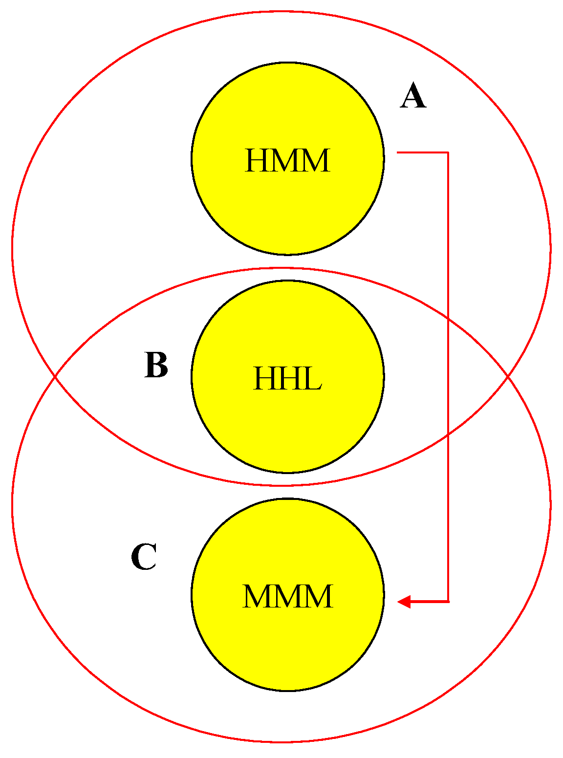
To explain the concept the three tenors show this example: 3 samples are compared, by the data A={H, M, M}, B={H, H, L}, C={M, M, M}. They write:
|
“To compare and order these samples we introduce a rule called ‘dominance criterion’, defined, case by case, on the basis of the characteristics of the monitored process. In accordance with this rule, if sample A dominates sample B, then sample A is preferred to sample B. As a result we can define a new ordinal scale whose levels are the positions of the samples in the ordered sample space. If there is no dominance relationship between sample A and sample B, they belong to the same ‘equivalence class’. The choice of the dominance criterion influences the resolution of the scale (i.e. the number of levels of the ordered sample space) and also the order of levels. For each process one or more dominance criterion may be established on the basic of the specific application”. “We begin analyzing the Pareto-dominance criterion. We state that sample X Pareto-dominates sample Y if all elements in Y do not exceed the corresponding elements in X, and at least one element in X exceeds sponding one in Y. This situation is formally denothe correted by . In case samples X and Y belong to the same equivalence class, i.e. no dominance relationship can be defined between them, we use the following notation: X≈Y”. “As we can see from figure, it is not possible to assign a well-defined position to samples A, B and C, because their intersection is not empty. The problem can be solved by introducing the concept of ‘semi-equivalence class’. A semi equivalence class is composed of equivalence classes whose intersections are not empty… |
Excerpt 16. Statements from “Ordered Sample Control Charts for Ordinal Variables”
The samples (figure 9) A and B form an “equivalence set”, as B and C do.
To avoid any “equivalence class” a more powerful “dominance criterion” is needed.
|
“As we can see from figure, it is not possible to assign a well-defined position to samples A, B and C, because their intersection is not empty. The problem can be solved by introducing the concept of ‘semi-equivalence class’. A semi equivalence class is composed of equivalence classes whose intersections are not empty… In general, Pareto dominance criterion gives a ‘poor’ ordering for the sample space of an ordinal quality characteristic. A more discerning criterion is the ‘rank dominance criterion’. Its introduction requires the definition of the concept of ‘optimal sample’. A sample is said to be optimal if all elements assume the highest level of an ordinal scale. In our example the optimal sample is HHH. For each sample we define a rank index which quantifies its positioning with regard to the optimal sample. The index is built in by adding up the numbers of scale levels contained between each sample value and the corresponding value of the optimal sample”. Consider the sample D={H, M, L}: its rank index is 3. “A high value of rank index corresponds to a ‘bad’ sample. All samples that are characterized by the same index belong to the same equivalence class. Therefore their positioning with respect to the optimal sample can be equivalently identified by the corresponding equivalence class. The number of elements of the new ordinal sample scale depends on the sample size and on the number of levels of the evaluation scale… Table V.6 (first column) reports all possible ordered samples of size n = 4, on an evaluation scale with t=3 levels. For each sample, the corresponding position on the resulting scales is reported (third column). The greater the position number, the higher the sample evaluation. A greater resolution, i.e. a larger number of levels, on the ordinal sample scale can be obtained by integrating the rank dominance criterion with the dispersion dominance criterion. This criterion allows distinguishing among samples belonging to the same equivalence class by analyzing sample dispersion. A lower position is associated with a greater dispersion. The fourth column of table V.6 reports the position of each sample in the new ordered sample space after the sequential application of the rank and the dispersion dominance criteria. As we can see, each ordered sample is associated with a different position; this is the greatest possible resolution”. |
Excerpt 17. Statements from “Ordered Sample Control Charts for Ordinal Variables”
All the samples with the same Rank Index belong to an “equivalence class”. “Therefore their positioning with respect to the optimal sample can be equivalently identified by the corresponding equivalence class”.
If the samples with size 4 of table 6 become of size 3 we have the Sample Space of the table 7:
Table 6.
15 samples (size 4) as “Ordered Sample Space” with Ranck Index and Positions (generated by dominance criteria).
Table 6.
15 samples (size 4) as “Ordered Sample Space” with Ranck Index and Positions (generated by dominance criteria).
| Sample Space | Rank Index | Position in the ordered sample space (equivalent class) [rank dominance criterion] |
Position in the ordered sample space (equivalent class) [rank & dispersion dominance criterion] |
| LLLL | 8 | 1st | 1st |
| MLLL | 7 | 2nd | 2nd |
| MMLL | 6 | 3rd | 4th |
| MMML | 5 | 4th | 6th |
| MMMM | 4 | 5th | 9th |
| HLLL | 6 | 3rd | 3rd |
| HMLL | 5 | 4th | 5th |
| HMML | 4 | 5th | 8th |
| HMMM | 3 | 6th | 11th |
| HHLL | 4 | 5th | 7th |
| HHML | 3 | 6th | 10th |
| HHMM | 2 | 7th | 13th |
| HHHL | 2 | 7th | 12th |
| HHHM | 1 | 8th | 14th |
| HHHH | 0 | 9th | 15th |
Table 7.
10 samples (size 3) as “Ordered Sample Space” with Ranck Index and Positions (generated by dominance criteria).
Table 7.
10 samples (size 3) as “Ordered Sample Space” with Ranck Index and Positions (generated by dominance criteria).
| Sample Space | Rank Index | Position in the ordered sample space (equivalent class) [rank dominance criterion] |
Position in the ordered sample space (equivalent class) [rank & dispersion dominance criterion] |
| LLL | 6 | 1st | 1st |
| MLL | 5 | 2nd | 2nd |
| MML | 4 | 3rd | 4th |
| MMM | 3 | 4th | 6th |
| HHH | 0 | 7th | 10th |
| HLL | 4 | 3rd | 3rd |
| HML | 3 | 4th | 5th |
| HMM | 2 | 5th | 8th |
| HHM | 1 | 6th | 9th |
| HHL | 2 | 5th | 7th |
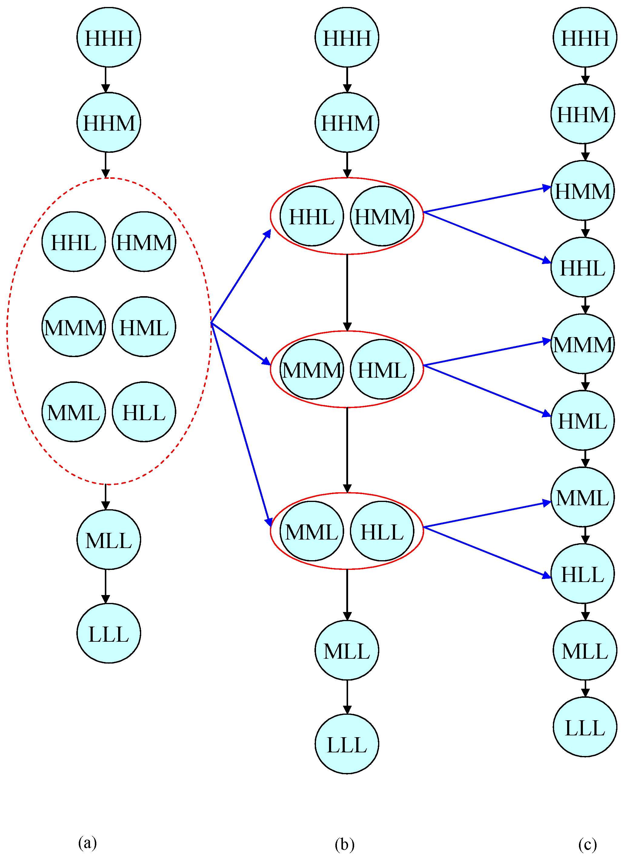
| “A vertical arrow represents a dominance relationship. A continuous ellipse represents an equivalence class, while a dashed ellipse represents a semi-equivalence class. The figures (a), (b) e (c) report respectively the results of the application of the Pareto-dominance, the rank dominance and the rank plus dispersion dominance criteria. The transverse arrows describe how each equivalence or semi-equivalence class is split by the application of a more discerning dominance criterion. The resolution of the ordered sample space varies with the considered dominance criterion. In accordance with a specific dominance criterion, sample charts report the positions of samples in the ordered sample space on the vertical axis. Given the particular meaning of sample charts, only the lower control limit (LCL) is defined. The central line (CL) represents the median of sample distribution. A set of initial samples is considered to determine the sample empirical frequency distribution. This empirical distribution (so a distribution exists!!!) is then used to calculate the lower control limit for a given type I error. Control limits are determined by empirical estimates of probabilities based on observed frequencies in a set of initial samples. Therefore, because the probabilities are estimated, the estimates contain errors, which could become significant for very small probabilities. A large initial set of samples or an alternative approach based on bootstrap techniques are needed to estimate the limits with a more reasonable accuracy”. |
Excerpt 18. Statements from “Ordered Sample Control Charts for Ordinal Variables”
We see this in the figure
Figure 9.
Ordered Sample Space samples of size 3, from the best (Up) to the least (Down): (a) “Pareto Dominance”, (b) “Rank Dominance”, (c) “Rank & Dispersion Dominance” (see Table 7).
Figure 9.
Ordered Sample Space samples of size 3, from the best (Up) to the least (Down): (a) “Pareto Dominance”, (b) “Rank Dominance”, (c) “Rank & Dispersion Dominance” (see Table 7).
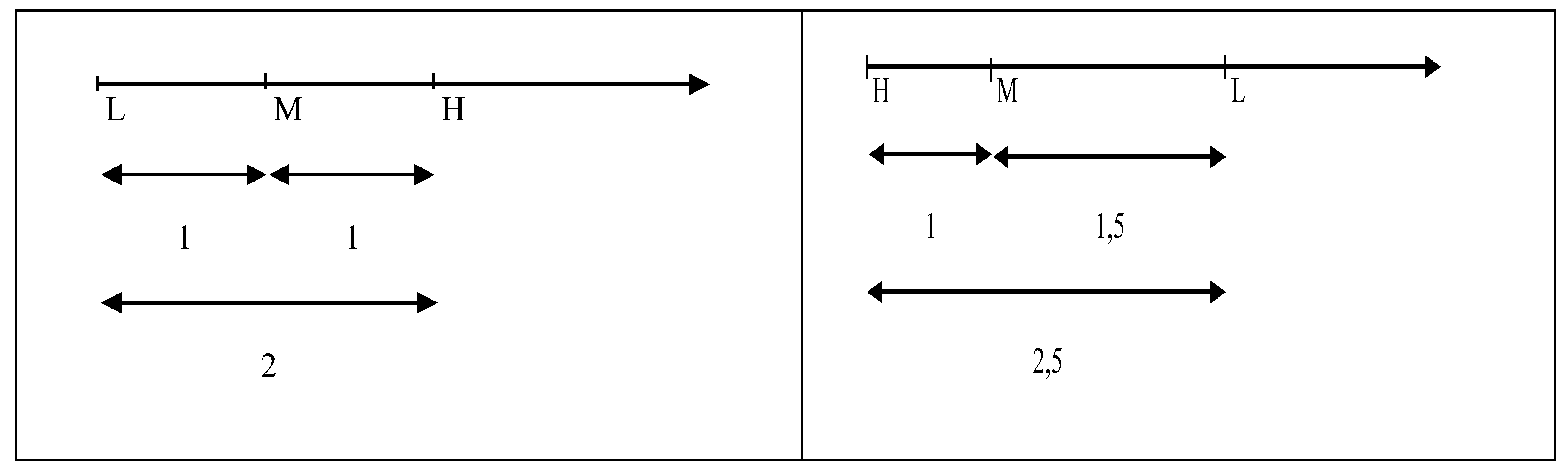
Now we do what is forbidden because it generates “distortion of the collected information”: we calarize the data, and use numbers in Qualitometro III. We show that we can assign numbers to any classification of the items (products, services, …) checked… and we get the same results as the “dominance criteria” [of the new three “tenors”]: numerisation provides NO distortion. Using the codification ‘Low’ = 0; ‘Medium’ = 1; ‘High’ = 2, one finds the results of the “rank dominance criterion”. [same distance between scale values] (on the left), while using the codification ‘Low’ = 2.5; ‘Medium’ = 1; ‘High’ = 0, one finds the results of the “rank and dispersion dominance criterion”. [different distance between scale values] (on the right)
Figure 10.
Scalarisation for Ordering the Sample Space (samples of size 3), “Rank Dominance” (b) in figure 9, “Rank & Dispersion Dominance” (c) in figure 9; see also Table 7.
Figure 10.
Scalarisation for Ordering the Sample Space (samples of size 3), “Rank Dominance” (b) in figure 9, “Rank & Dispersion Dominance” (c) in figure 9; see also Table 7.
With numbers we get the same results …
Notice that the complete sample space, generated by 3 items (sample size) inspected and evaluated on a 3 levels scale (L, M, H), has 27=33 states; naming X the Random Variable “result of the inspection” we can define the probabilities pL=P[X=L], pM=P[X=M], pH=P[X=H] of the events [X=L], [X=M] and [X=H] for any item inspected, and derive that each state out of the 27 has the probability pstate depending on the probabilities of the levels scale (L, M, H) of each inspected items. Notice that our inspection is like a random experiment consisting of a series of independent trials ad so to find the probability pstate we use the joint probability distribution for multiple discrete random variables. The outcome from each trial is categorized into one of 3 classes (L, M, H). The random variables of interest count the number of outcomes in each class.
In the next session we will see the results on the Q III.
3. Results
In this section, firstly, we provide the scientific analysis of about the Q III method. The readers can see that “scalarisation” does not provide any harm: The results are equivalent in the various scales due to the “isomorphism”.
3.1. Results on the Qualitometro III (Q III)
Before we considered the complete sample space, generated by 3 items (sample size) inspected and evaluated on a 3 levels scale (L, M, H) with its 27=33 states.
Now we consider the complete sample space, generated by 4 items (sample size) inspected and evaluated on a 3 levels scale (L, M, H), has 81=43 states; naming X the Random Variable “result of the inspection” we can define the probabilities pL=P[X=L], pM=P[X=M], pH=P[X=H] of the events [X=L], [X=M] and [X=H] for any item inspected, and derive that each state out of the 81 has the probability pstate depending on the probabilities of the levels scale (L, M, H) of each inspected items.
The joint probability distribution for multiple discrete random variables is the “Multinomial Probability Mass” where n is the sample size.
If one uses the multinomial, with n=4 (as in table 5) and the “scalarisation” in figure 10, he can find the probability of each "class of equivalence": that allows the calculation of the UCL and LCL of the control charts.
You get the same results if you use, as well, either L=15, M=10, H=4 or L=4, M=10, H=15; try and see!
Count the numbers nL, nM, nH of the levels scale (L, M, H) of each sample, using the “scalarisation” in figure 10; compute the “inner product” nL *L + nM *H, which is a number (of a “metric space”): with the left “scalarisation” you get the "equivalence classes" of the “rank dominance criterion”, while with the right “scalarisation” you get the "equivalence classes" of the “rank & dispersion dominance criterion”: see the Table 6.
See the probability distributions in the figures 11 and 13 and the “Control Charts” in the figures 12 and 14.
Figure 11.
Probability of Ordered Sample Space “states” ("classes of equivalence") and (samples of size 4): same as with the “Rank Dominance”.
Figure 11.
Probability of Ordered Sample Space “states” ("classes of equivalence") and (samples of size 4): same as with the “Rank Dominance”.
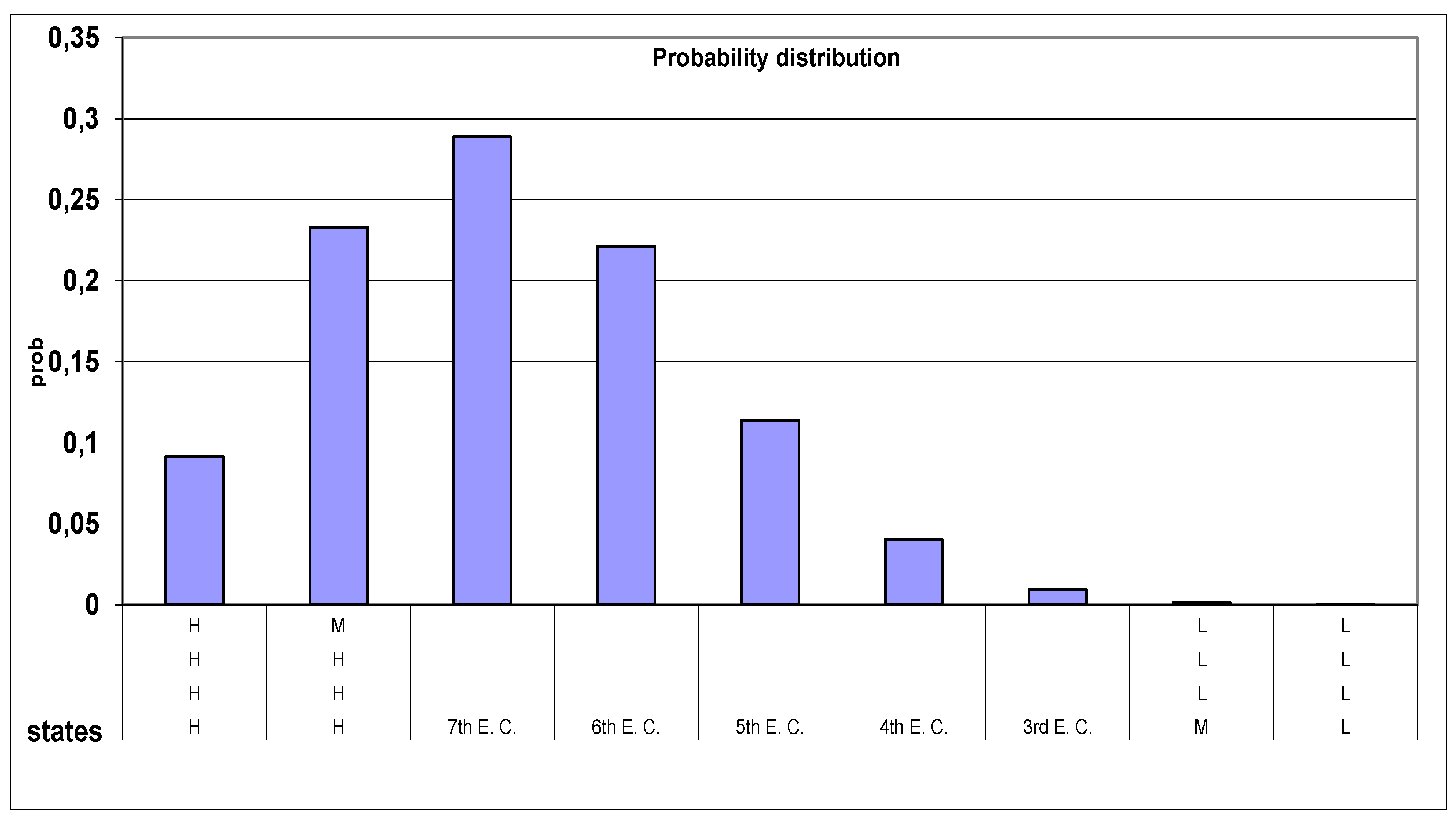
Figure 12.
Control Chart (with “states” "classes of equivalence") and (samples of size 4) for “Rank Dominance”.
Figure 12.
Control Chart (with “states” "classes of equivalence") and (samples of size 4) for “Rank Dominance”.
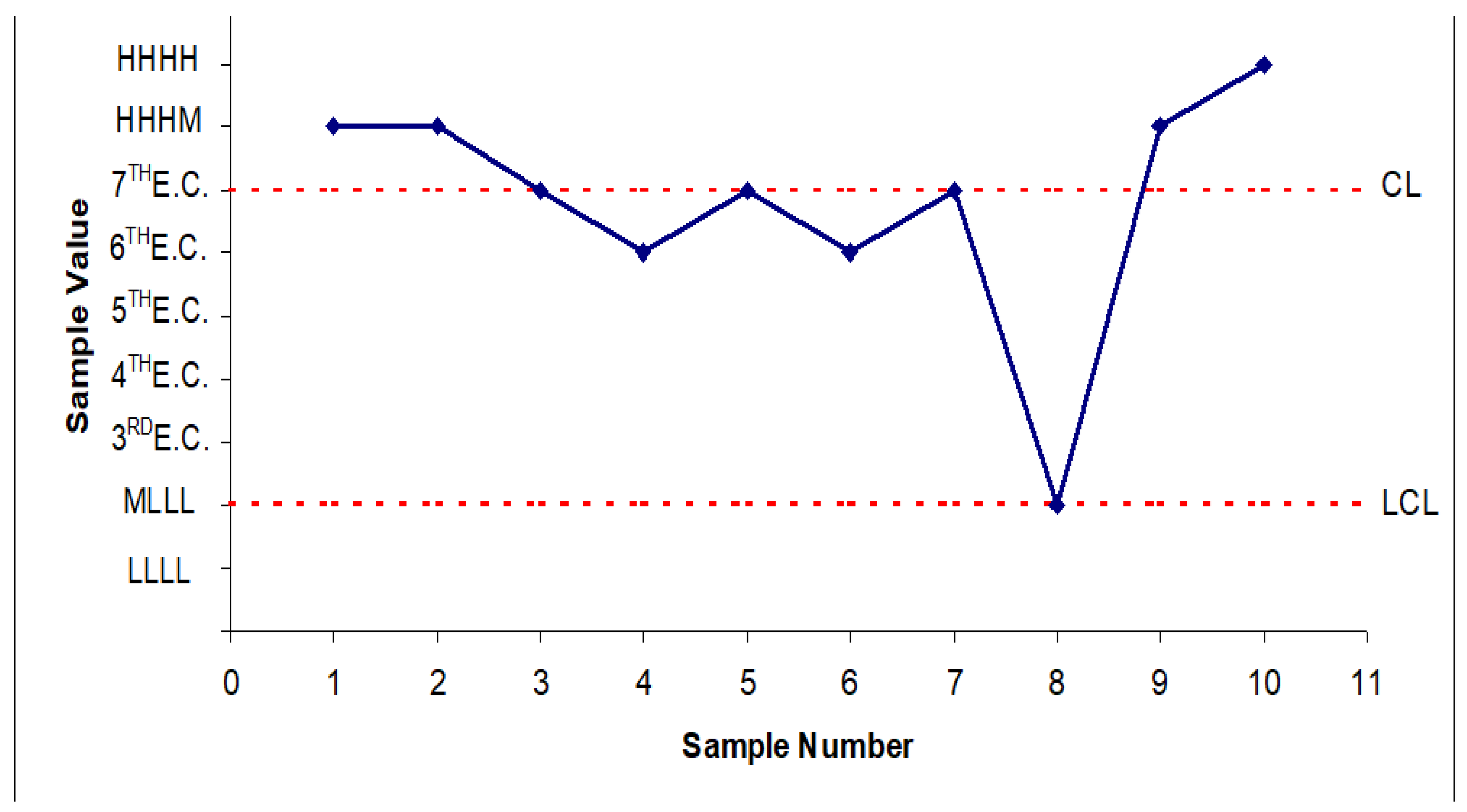
Figure 13.
Probability of Ordered Sample Space “states” ("classes of equivalence") and (samples of size 4): same as with the “Rank & Dispersion Dominance”.
Figure 13.
Probability of Ordered Sample Space “states” ("classes of equivalence") and (samples of size 4): same as with the “Rank & Dispersion Dominance”.
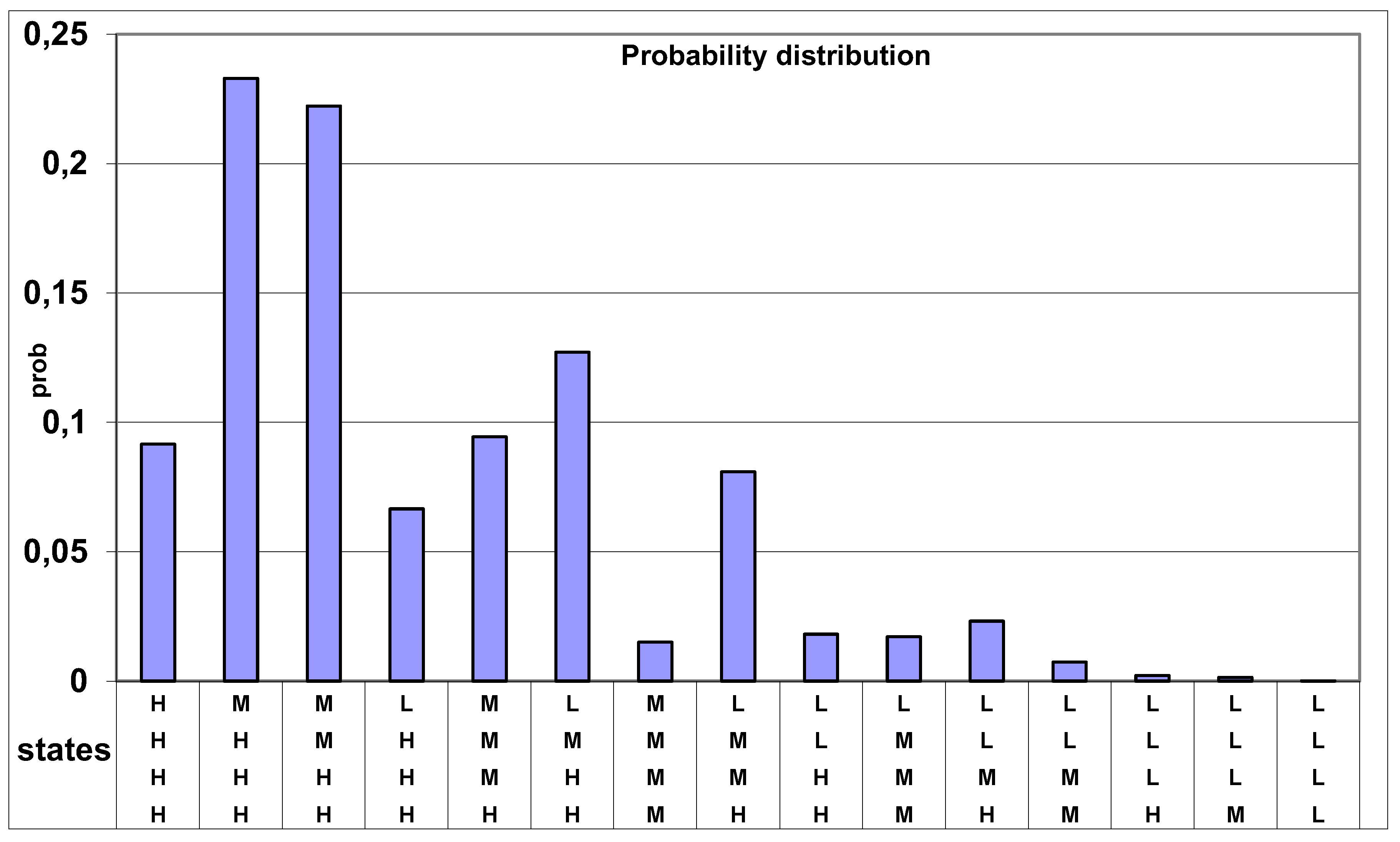
Figure 14.
Control Chart (with “states” "classes of equivalence") and (samples of size 4) for “Rank & Dispersion Dominance”.
Figure 14.
Control Chart (with “states” "classes of equivalence") and (samples of size 4) for “Rank & Dispersion Dominance”.

Is there any doubt that one can use numbers and that there is a distribution connected with the sampling? Is there any doubt that
- ⇒
- "The numerical codification implies fixing the distances among scales levels, thus converting the ordinal scale into a cardinal one; the second is related to the absence of consistent criteria for the selection of the type of numerical conversion [are consistent the "dominance criteria" of the new three "tenors"?????]. It is obvious that changing the numerical encoding [as the "dominance criteria" of the new three "tenors"] may determine a change in the obtained results. In this way the analyst directly influences the acceptance of results.
- ⇒
- Therefore, any conclusions drawn from the analysis on ‘equivalent’ numerical [as the "dominance criteria" of the new three "tenors"] data could be partially or wholly distorted "
- ⇒
- “By the adopted criteria, the example presents some significant differences compared with the approach based on the numeric codification of levels. Using different criteria the difference between the proposed approach and the traditional one becomes more evident, such as for the ordinal sample charts. Furthermore, ordinal range charts also allow a process positioning analysis. A good quality process will present a concentration of samples at the lowest positions of the ordinal range space scale”.
- ⇒
- “The paper presents two new control charts for the process control of quality characteristics evaluated on an ordinal scale, without exploiting an artificial conversion of scale levels. The basic concept of the charts is the ordering of the sample space of the quality characteristic at hand.
- ⇒
- Charts do not suffer from the poor resolution shown by other linguistic charts [while BEFORE for Qualitometro II they said, some years before, that they were fantastic!], where the original evaluation scale is used to evaluate samples”.
- ⇒
- “No distributional shape is assumed for the population (universe) of evaluations”. [a distribution exists and it is the multinomial!]
are FALSE statements?
Only the incompetent "Peer Reviewers" of the magazines "Quality Engineering" and "Quality and Reliability Engineering International" do not understand that.
A question is eventually important: why, for the same data, collected for the "Valdese Hospital", the importance of criteria was very important in Qualitometro II, while it was no longer important in Qualitometro III?
Then, what can Fausto Galetto do? Only reminding professors they must not teach wrong ideas! But professors of the "international scientific community" are deaf: "none so deaf as those that won't hear".
Remember that R. P. Feynman, Nobel laureate in physics, once said, “You do not know anything until you have practiced.” Your ability to solve problems will be one of the main tests of your knowledge. It is essential that you understand basic concepts and principles before attempting to solve problems.
Shewhart (1931) stated that "a controlled quality is a variable quality". Therefore "Quality achievement", needs understanding of variability. Theory only provides this understanding. To understand, theory is necessary: "Experience without theory teaches nothing" (Deming 1982). Deming has been always very clear on this point: he said about his days working at Western Electric Co. (1927) [when Shewhart and Rossbacher were there] "My esteem for him has increased year by year. He had respect for theory. ... He had no use for the word practical". Therefore, to achieve that point "variable quality, but yet controlled" theory is necessary.
The proof? It's here!
According to prof. F. Franceschini (Politecnico di Torino), papers published in Quality Magazines [8] are, by definition, good papers: we saw that it is not true.
He did not read [10,11,12,13,14,15,16,17,18,19,20,21,22,23,24,25,26,27,28,29,30,31,32,33,34,35,36,37,38,39,40,41,42,43,44,45,46,47,48,49,50,51,52,53,54,55,56,57,58,59,60,61,62,63,64,65,66,67,68,69,70,71,72,73,74,75,76,77,78,79,80,81,82,83,84,85] with due care and Logic!
He did not consider the Theory of “tests of hypotheses” and stochastic processes [11,12,13,14,15,16,17,18,19,20,21,22,23,24,25,26,27,28,29,30,31,32,33,34,35,36,37,38,39,40,41,42,43,44,45,46,47,48,49,50] and Galilei ideas [51,52].
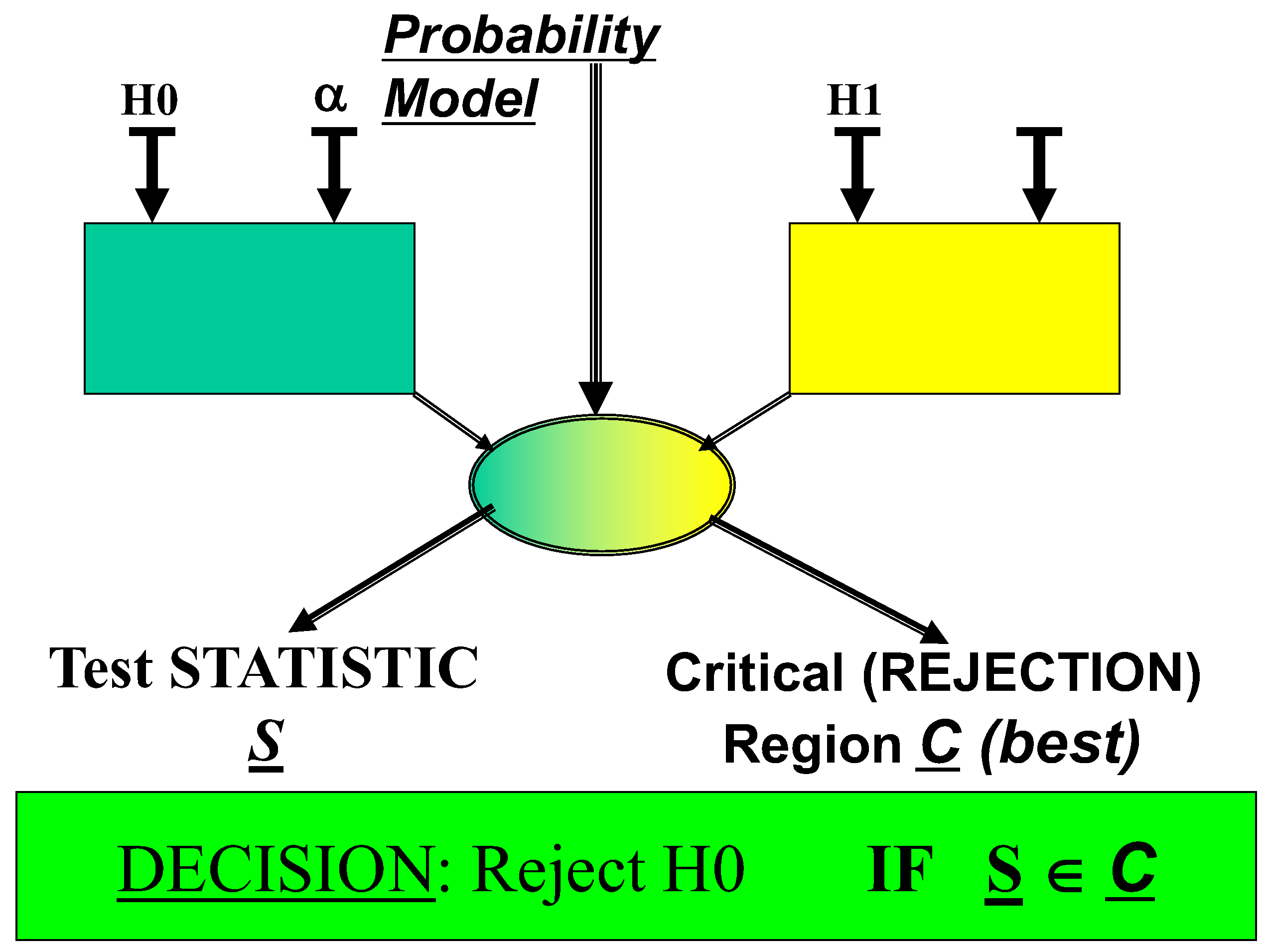
The framework of a test of hypothesis is depicted in the figure 1.
Figure 15.
The pictorial framework of a Statistical Hypothesis (based on a Probability Model of Stochastic Processes for Control Charts).
Figure 15.
The pictorial framework of a Statistical Hypothesis (based on a Probability Model of Stochastic Processes for Control Charts).
3.2. Control Charts for “for Monitoring the Exponential Process with Estimated Parameter”
Now we see that the drawbacks in papers for Control Charts are not limited to case such those of table 1 and fuzzy-linguistic variables, as shown before.
The Journals [8] published several wrong papers; the last found (December 2024) by FG is “An enhanced EWMA chart with variable sampling interval scheme for monitoring the exponential process with estimated parameter”, (Yajie Bai , Jyun-You Chiang , Wen Liu * & Zhengcheng Mou), www.nature.com/scientificreports
In their Abstract the authors write:
|
Control charts have been used to monitor product manufacturing processes for decades. The exponential distribution is commonly used to fit data in research related to healthcare and product lifetime. This study proposes an exponentially weighted moving average control chart with a variable sampling interval scheme to monitor the exponential process, denoted as a VSIEWMA-exp chart. The performance measures are investigated using the Markov chain method. In addition, an algorithm to obtain the optimal parameters of the model is proposed. We compared the proposed control chart with other competitors, and the results showed that our proposed method outperformed other competitors. Finally, an illustrative example with the data concerning urinary tract infections is presented. Keywords Exponential process, Estimated parameter, Exponentially weighted moving average, Variable sampling interval, Markov chain method, Optimization algorithm design |
Excerpt 19. Statements from “An enhanced EWMA chart with … estimated parameter”
Notice the statement “Finally, an illustrative example with the data concerning urinary tract infections is presented”.
This case was shown in many papers and considered by FG in several of his papers. The control charts proposed by those authors are wrong [53,54,55,56,57,58,59,60,70,71,72,73,74,75,76,77,78,79,80,81].
See the excerpt 20:
 |
Excerpt 20. Statements from “An enhanced EWMA chart with … estimated parameter”
4. Discussion
We decided to use the data from the papers of table 1 and the paper in section 3and the analysis by the authors.
Using the Theory we got different results from those authors: the cause is that they use the Probability Limits of the PI (Probability Interval) as they were the Confidence Limits (Control Limits of the Control Charts).
The proof of the confusion between the intervals L-------U (Probability Interval) and LCL-------UCL (Confidence Interval) in the domain of Control Charts (for Process Management) highlight the importance and novelty of these ideas in the Statistical Theory and in the applications.
For the “location” parameter in the CCs, from the Theory, we know that two mean (parameter), q=1,2, …, n, and any other mean (parameter), r=1,2, …, n, are different, with risk α, if their estimates are not both included in their common Confidence Interval as the CI of the grand mean (parameter) is.
Let’s consider the Shewhart formulae and apply them to a “Normal model” (due to CLT, and assuming known variance), sequentially we can write the “real” fixed interval L----U comprising the RV (vertical interval) and the Random Interval comprising the unknown mean (horizontal interval) (fig. 16)
When the RV assume its determination (numerical value) (grand mean) the Random Interval becomes the Confidence Interval for the parameter μ, with CL=1-α: risk α that the horizontal line does not comprise the “mean” μ.
This is particularly important for the Individual Control Charts for Exponential, Weibull, Inverted Weibull, General Inverted Weibull, Maxwell and Gamma distributed data: this is what Deming calls “Profound Knowledge (understanding variation)” [14,15]. The Confidence Interval, the realisation of the horizontal Random Interval.
The case we considered shows clearly that the analyses, in the Process Management, taken so far have been wrong and the decisions have been misleading, when the collected data follow a Non-Normal distribution.
Since a lot of papers (related to Exponential, Weibull, Inverted Weibull, General Inverted Weibull, Maxwell and Gamma distributions), with the same problem as that of “The garden of flowers” [83], are published in reputed Journals we think that the “alternative” title “History is written by the winners. Reflections on Control Charts for Process Control” is suitable for this paper: the authors of the wrong papers [83] are the winners.
Figure 16.
Probability Interval L---U (vertical line) versus Random Intervals comprising the “mean” μ (horizontal random variable lines), for Normally distributed RVs (based on a Probability Model of Stochastic Processes for Control Charts).
Figure 16.
Probability Interval L---U (vertical line) versus Random Intervals comprising the “mean” μ (horizontal random variable lines), for Normally distributed RVs (based on a Probability Model of Stochastic Processes for Control Charts).
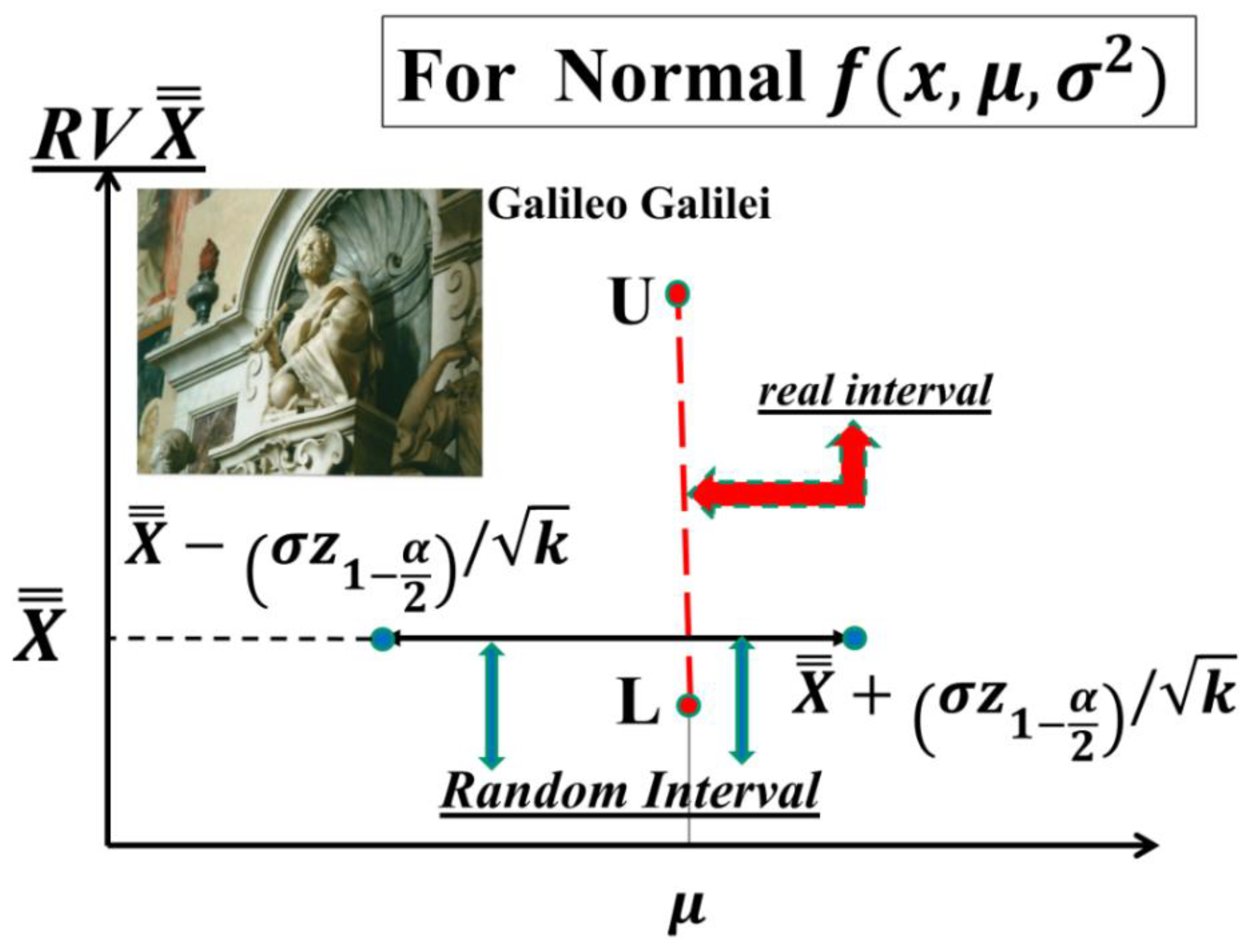
Further studies should consider other distributions which cannot be transformed into the above distributions considered before.
5. Conclusions
With our figures (and the Appendix, that is a short extract from the “Garden … [83]”) we humbly ask the readers to look at the references and find how much the author has been fond of Quality and Scientificness in the Quality (Statistics, Mathematics, Thermodynamics, …) Fields.
The errors, in the “Garden … [83]”, are caused by the lack of knowledge of sound statistical concepts about the properties of the parameters of the parent distribution generating the data, and the related Confidence Intervals. For the I-CC_TBE the computed Control Limits (which are actually the Confidence Intervals), in the literature are wrong due to lack of knowledge of the difference between Probability Intervals (PI) and Confidence Intervals (CI). Therefore, the consequent decisions about Process IC and OOC are wrong.
RIT is able to solve various problems in the estimation (and Confidence Interval evaluation) of the parameters of distributions. The basics of RIT can be found in [39,40,41,42,43,44,45].
Following the scientific ideas of Galileo Galilei, the author many times tried to compel several scholars to be scientific (Galetto 1981-2025). Only Juran appreciated the author’s ideas when he mentioned the paper “Quality of methods for quality is important” at the plenary session of EOQC Conference, Vienna. [48]
RIT can prove that the “linguistic charts” and the T Charts, for rare events and TBE (Time Between Events), used in the software Minitab, SixPack, JMP or SAS are wrong. So doing the author increased the h-index of the mentioned authors who published wrong papers.
RIT allows the scholars (managers, students, professors) to find sound methods also for the ideas shown by Wheeler in Quality Digest documents.
Figure 17.
Knowledge versus Ignorance, in Tools and Methods.
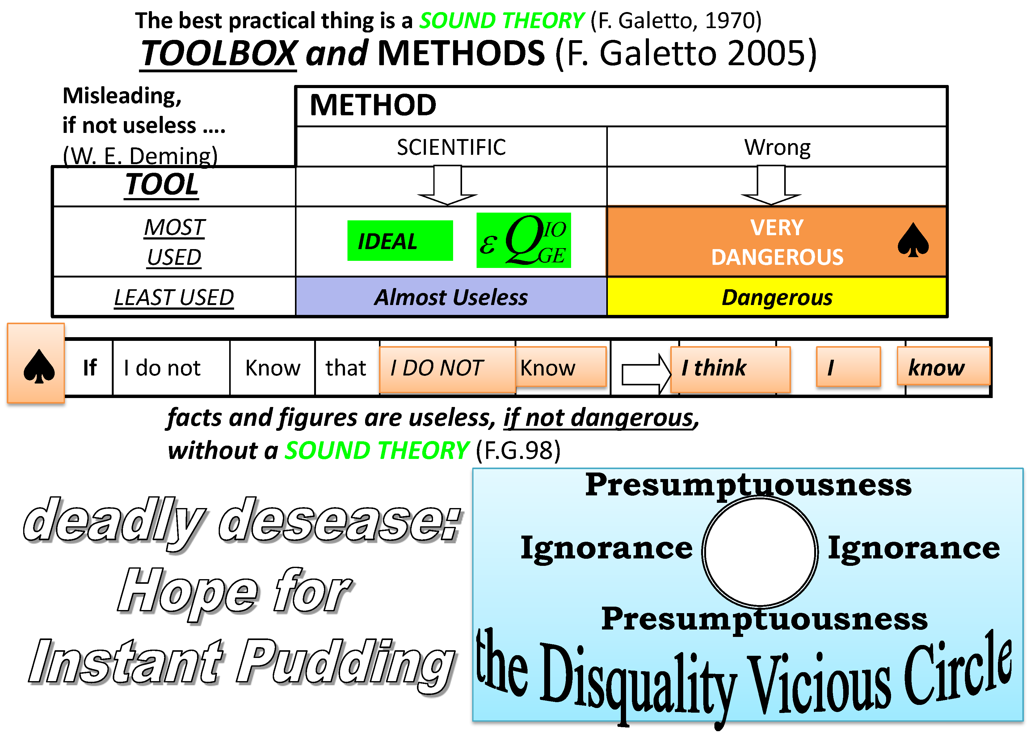
We informed the authors and the Journals who published wrong papers by writing various letters to the Editors…: no “Corrective Action”, a basic activity for Quality has been carried out by them so far. The same happened for Minitab Management. We attended a JMP forum in the JMP User Community and informed them that their “Control Charts for Rare Events” were wrong: they preferred to stop the discussion, instead to acknowledge the JMP faults.
So, dis-quality continues to be diffused people and people continue taking wrong decisions…
Deficiencies in products and methods generate huge cost of Dis-quality (poor quality) as highlighted by Deming and Juran. Any book and paper are products (providing methods): their wrong ideas and methods generate huge cost for the Companies using them. The methods given here provide the way to avoid such costs, especially when RIT gives the right way to deal with Preventive Maintenance (risks and costs), Spare Parts Management (cost of unavailability of systems and production losses), Inventory Management, cost of wrong analyses and decisions.
We think that we provided the readers with the belief that Quality of Methods for Quality is important.
The reader should remember the Deming’s statements.
Unfortunately, many authors do not know Scientifically the role (concept) of Confidence Intervals for Hypothesis Testing.
Therefore, they do not extract the maximum information form the data in the Process Control.
Control Charts are a means to test the hypothesis about the process states, H0={Process In Control} versus H1={Process Out Of Control}, with stated risk α=0.0027.
We have a big problem about Knowledge: sound Education is needed.
We think that the figure 17 conveys the fundamental ideas about the need of Theory for devising sound Methods, to be used in real applications in order to avoid the Dis-quality Vicious Circle.
Humbly, given our commitment to Quality and our long-life love for it [1,2,3,4,5,6,7,8,9,10,11,12,13,14,15,16,17,18,19,20,21,22,23,24,25,26,27,28,29,30,31,32,33,34,35,36,37,38,39,40,41,42,43,44,45,46,47,48,49,50,51,52,53,54,55,56,57,58], we would venture to quote Voltaire:
“It is dangerous to be right in matters on which the established men are wrong.” because “Many are destined to reason wrongly; others, not to reason at all; and others, to persecute those who do reason.” So, “The more often a stupidity is repeated, the more it gets the appearance of wisdom.” and “It is difficult to free fools from the chains they revere.”
Let’s hope that Logic and Truth prevail and allow our message to be understood.
The objective of collecting and analysing data is to take the right action. The computations are merely a means to characterize the process behaviour. However, it is important to use the right Control Limits take the right action about the process states, i.e., In Control versus Out Of Control.
On July-December 2024 we again verified (through several new downloaded papers, not shown here) that the Pandemic Disease about the (wrong) Control Limits, that are actually the Probability Limits of the PI is still present …
There will be any chance that the Pandemic Disease ends? The only way out is Knowledge… (fig. 17): Deming’s Profound Knowledge, Metanoia, Theory.
There is no “free lunch”: metanoia and study are needed and necessary.
Funding
This research received no external funding.
Data Availability Statement
“MDPI Research Data Policies” at https://www.mdpi.com/ethics.
Conflicts of Interest
The author declares no conflicts of interest.
References
- R. E. Bellman und L. A. Zudeh, Decision-Making in a Fuzzy Environment, Report No ERL-69-8, NASA.
- Zadeh, I. (1976) The concept of linguistic variable and application to approximate reasoning, Inf. Science.
- Belmann, R., Zadeh, I. (unknown) Decision making in a fuzzy environment, NASA CR-1594.
- Yager, R. (1981) New methodology for ordinal decision based on fuzzy sets, Decision Sciences, 12, 589-600.
- Yager, R.R. Non-numeric multi-criteria multi-person decision making. Group Decis. Negot. 1993, 2, 81–93. [CrossRef]
- Yager, R., Filev, D. P. (1994). Essentials of Fuzzy Modeling and Control. New York, USA: J. Wiley.
- Zadeh, L. Polak, E. (1969) System Theory, McGraw-Hill.
- Journals: Quality and Reliability Engineering International, Quality Engineering,, Reliability Engineering and System Safety, IIE Transactions, Quality Technology and Quantitative Management, Quality & Quantity, J. of Applied Statistics, J. of Quality Technology, J. of Statistical Planning and Inference, J. of Statistical Computation and Simulation, International J. of Production Research, J. of the American Statistical Association, International J. for Quality Research, J. of Quality Technology, J. of Statistical Theory and Practice, J. of Statistical Theory and Applications, J. of Applied Probability and Statistics, International J. of Advanced Manufacturing Technology, J. of Systems Science and Information, European J. of Operational Research, J. of Nonparametric Statistics, J, of the Japanese Society of Computational Statistics, Communications in Statistics - Simulation and Computation, Statistics and Probability Letters, Communications in Statistics - Theory and Methods, Computational Statistics, Computational Statistics & Data Analysis, www.nature.com/scientificreports.
- Bass, F.M. A new product growth for model consumer durables. Manag. Sci. 1969, 15, 215–227. [CrossRef]
- Bellman, R. (1970) Introduction to Matrix Analysis, 2nd ed., McGraw-Hill.
- Belz, M. Statistical Methods in the Process Industry: McMillan; 1973.
- Casella, Berger, Statistical Inference, 2nd edition: Duxbury Advanced Series; 2002.
- Cramer, H. Mathematical Methods of Statistics: Princeton University Press; 1961.
- Deming W. E., Out of the Crisis, Cambridge University Press; 1986.
- Propst, A.L.; Deming, W.E. The new economics for industry, government, education. Technometrics 1996, 38, 294. [CrossRef]
- Dore, P., (1962) Introduzione al Calcolo delle Probabilità e alle sue applicazioni ingegneristiche, Casa Editrice Pàtron, Bologna.
- Cramer, H., (1961) Mathematical Methods of Statistics, Princeton University Press.
- Ziegel, E.R.; Juran, J.M.; Gryna, F.M. Quality Control Handbook, 4th. Technometrics 1990, 32, 97. [CrossRef]
- Kendall, Stuart, (1961) The advanced Theory of Statistics, Volume 2, Inference and Relationship, Hafner Publishing Company.
- Meeker, W., Hahn, G.., Escobar, L. Statistical Intervals: A Guide for Practitioners and Researchers. John Wiley & Sons. 2017.
- Mood, Graybill, Introduction to the Theory of Statistics, 2nd ed.: McGraw Hill; 1963.
- Papoulis, A.; Saunders, H. Probability, Random Variables and Stochastic Processes. J. Vib. Acoust. 1989, 111, 123–125. [CrossRef]
- Rao, C. R., (1965) Linear Statistical Inference and its Applications, Wiley & Sons.
- Rozanov, Y., (1975) Processus Aleatoire, Editions MIR, Moscow, (traduit du russe) Ryan, T. P., (1989) Statistical Methods for Quality Improvement, Wiley & Sons.
- Saaty, T. (1969) Mathematical Methods of Operations Research, McGraw-Hill.
- Saaty, T., Bram, J. (1964) Nonlinear Mathematics, McGraw-Hill.
- Shewhart W. A., (1931) Economic Control of Quality of Manufactured Products, D. Van Nostrand Company.
- Shewhart W.A., (1936) Statistical Method from the Viewpoint of Quality Control Graduate School, Washington.
- D. J. Wheeler, “The normality myth”, Online available from Quality Digest.
- D. J. Wheeler, “Probability limits”, Online available from Quality Digest.
- D. J. Wheeler, “Are you sure we don’t need normally distributed data?” Online available from Quality Digest.
- D. J. Wheeler, “Phase two charts and their Probability limits”, Online available from Quality Digest.
- Feller, W. (1967) An Introduction to Probability Theory and its Applications, Vol. 1, 3rd Ed. Wiley.
- Feller, W. (1965) An Introduction to Probability Theory and its Applications, Vol. 2, Wiley.
- Parzen, E. (1999) Stochastic Processes, Society for Industrial and Applied Mathematics.
- Jones, P., Smith, P. (2018) Stochastic Processes An Introduction, 3rd Ed. CRC Press.
- Knill, O. Probability Theory and Stochastic Processes with Applications; World Scientific Pub Co Pte Ltd: Singapore, Singapore, 2016; ISBN: .
- Shannon, Weaver (1949) The Mathematical Theory of Communication, University of Illinois Press.
- Galetto, F., (1981, 84, 87, 94) Affidabilità Teoria e Metodi di calcolo, CLEUP editore, Padova (Italy).
- Galetto, F., (1982, 85, 94) “Affidabilità Prove di affidabilità: distribuzione incognita, distribuzione esponenziale”, CLEUP editore, Padova (Italy).
- Galetto, F., (1995/7/9) Qualità. Alcuni metodi statistici da Manager, CUSL, Torino (Italy).
- Galetto, F., (2010) Gestione Manageriale della Affidabilità”, CLUT, Torino (Italy).
- Galetto, F., (2015) Manutenzione e Affidabilità, CLUT, Torino (Italy).
- Galetto, F., (2016) Reliability and Maintenance, Scientific Methods, Practical Approach”, Vol-1, www.morebooks.de.
- Galetto, F., (2016) Reliability and Maintenance, Scientific Methods, Practical Approach”, Vol-2, www.morebooks.de.
- Zhang, H.; Guo, J.; Zhou, L. Hope for the Future: Overcoming the DEEP Ignorance on the CI (Confidence Intervals) and on the DOE (Design of Experiments. Sci. J. Appl. Math. Stat. 2015, 3, 70. [CrossRef]
- Galetto, F., 2019, Statistical Process Management, ELIVA press ISBN 9781636482897.
- Galetto, F., (1989) Quality of methods for quality is important, EOQC Conference, Vienna,.
- Galetto, F., (2015) Management Versus Science: Peer-Reviewers do not Know the Subject They Have to Analyse, Journal of Investment and Management. Vol. 4, No. 6, pp. 319-329. [CrossRef]
- Galetto, F. The first step to Science Innovation: Down to the Basics. Sci. Innov. 2015, 3, 81. [CrossRef]
- Galilei, Galileo, Saggiatore, 1623 (in Italian).
- Galilei, Galileo, Dialogo sopra i due massimi sistemi del mondo, Tolemaico e Copernicano (Dialogue on the two Chief World Systems), 1632 (in Italian).
- Galetto, F. Minitab T charts and quality decisions. J. Stat. Manag. Syst. 2021, 25, 315–345. [CrossRef]
- Galetto, F. Minitab T charts and quality decisions. J. Stat. Manag. Syst. 2021, 25, 315–345. [CrossRef]
- Galetto, F., (2012) Six Sigma: help or hoax for Quality?, 11th Conference on TQM for HEI, Israel.
- Galetto, F., (2020) Six Sigma_Hoax against Quality_Professionals Ignorance and MINITAB WRONG T Charts, HAL Archives Ouvert, 2020.
- Galetto, F., (2021) Control Charts for TBE and Quality Decisions, submitted.
- Galetto F. (2022), “Affidabilità per la manutenzione Manutenzione per la disponibilità”, tab edezioni, Roma (Italy), ISBN 978-88-92-95-435-9, www.tabedizioni.it.
- Scholar, P.L.A.P.d.T.I.; Galetto, F. ASSURE: Adopting Statistical Significance for Understanding Research and Engineering. 2021, 1–10. [CrossRef]
- Galetto F. (2023) Control Charts, Scientific Derivation of Control Limits and Average Run Length, International Journal of Latest Engineering Research and Applications (IJLERA) ISSN: 2455-7137 Volume – 08, Issue – 01, January 2023, PP – 11-45.
- Galetto, F. GIQA the Golden Integral Quality Approach: from Management of Quality to Quality of Management. Total. Qual. Manag. 1999, 10, 17–35. [CrossRef]
- Galetto, F., (2004) Six Sigma Approach and Testing, ICEM12 –12th International Conference on Experimental Mechanics, 2004, Bari Politecnico (Italy).
- Galetto, F., (2006) Quality Education and quality papers, IPSI, Marbella (Spain).
- Galetto, F., (2006) Quality Education versus Peer Review, IPSI, Montenegro.
- Galetto, F., (2006) Does Peer Review assure Quality of papers and Education? 8th Conference on TQM for HEI, Paisley (Scotland).
- Montgomery D., (1996, 2009, 2011) Introduction to Statistical Quality Control, Wiley & Sons (wrong definition of the term "Quality", and many other drawbacks in wrong applications).
- Montgomery D., (2019) “Introduction to Statistical Quality Control”, 8th Wiley & Sons.
- Galetto, F., “Design Of Experiments and Decisions, Scientific Methods, Practical Approach”, 2016, www.morebooks.de.
- Galetto, F., “The Six Sigma HOAX versus the versus the Golden Integral Quality Approach LEGACY”, 2017, www.morebooks.de.
- Galetto, F., “Quality Education on Quality for Future Managers”, 1st Conference on TQM for HEI (Higher Education Institutions), 1998, Toulone (France).
- Galetto, F., “Quality Education for Professors teaching Quality to Future Managers”, 3rd Conference on TQM for HEI, 2000, Derby (UK).
- Galetto, F., “Quality, Bayes Methods and Control Charts”, 2nd ICME 2000 Conference, 2000, Capri (Italy).
- Galetto, F., “Looking for Quality in "quality books", 4th Conference on TQM for HEI, 2001, Mons (Belgium).
- Galetto, F. Quality and Control Carts: Managerial assessment during Product Development and Production Process”. Automotive and Transportation Technology Congress and Exposition. LOCATION OF CONFERENCE, SpainDATE OF CONFERENCE; .
- Galetto, F. Quality QFD and control charts: a managerial assessment during the product development process”. Automotive and Transportation Technology Congress and Exposition. LOCATION OF CONFERENCE, SpainDATE OF CONFERENCE; .
- Galetto, F., “Business excellence Quality and Control Charts”, 7th TQM Conference, 2002, Verona (Italy).
- Galetto, F., “Fuzzy Logic and Control Charts”, 3rd ICME 2002 Conference, Ischia (Italy).
- Galetto, F., “Analysis of "new" control charts for Quality assessment”, 5th Conference on TQM for HEI, 2002, Lisbon (Portugal).
- Galetto, F., “The Pentalogy, VIPSI, 2009, Belgrade (Serbia).
- Galetto, F., The Pentalogy Beyond, 9th Conference on TQM for HEI, 2010, Verona (Italy).
- Scholar, P.L.A.P.d.T.I.; Galetto, F. ASSURE: Adopting Statistical Significance for Understanding Research and Engineering. 2021, 1–10. [CrossRef]
- Galetto, F., (2024), News on Control Charts for JMP, Academia.edu.
- Galetto, F., Papers and Documents in Academia.edu, 2015-2025.
- Galetto, F., Several Papers and Documents in the Research Gate Database, 2014.
- Giordani, A., (2011), Lezioni di Filosofia della Scienza, EduCatt, ISBN 978-88-8311-787-9.
Figure 1.
Qualitometro pictorial format for collecting data (with Linguistic Variables): actual data.
Figure 1.
Qualitometro pictorial format for collecting data (with Linguistic Variables): actual data.
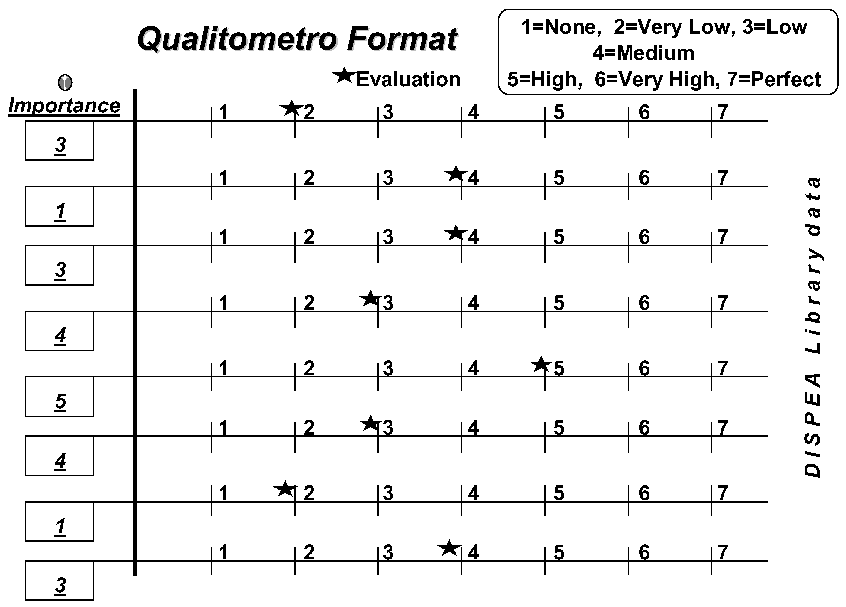
Table 1.
The papers considered in the analysis.
| Franceschini F. et al. | On-line service quality control: The ‘Qualitometro’ method | Quality Engineering | 1999 | QI |
| Franceschini F. et al. | Service Qualimetrics: The Qualitometro II method | Quality Engineering | 1999 | QII |
| Franceschini F. et al. | Control chart for linguistic variables: A method based on the use of linguistic quantifiers | International Journal of Production Research | 1999 | |
| Franceschini F. et al. | Qualitative ordinal scales: The concept of ordinal range | Quality Engineering | 2004 | |
| Franceschini F. et al. | Ordered Sample Control Charts for Ordinal Variables (named here Qualitometro III) | Quality and Reliability Engineering International | 2005 | QIII |
Table 3.
The Matrices R and V.
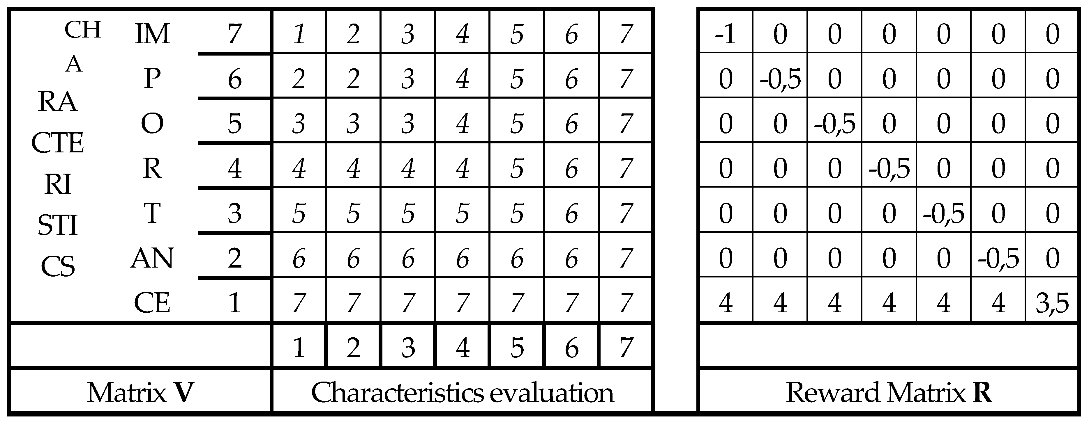
Table 5.
Data collected on 10 samples (size 4) of mechanical pieces for X-R Control Chart and Linguistic Charts (Qualitometro II)
Table 5.
Data collected on 10 samples (size 4) of mechanical pieces for X-R Control Chart and Linguistic Charts (Qualitometro II)
| Original data | Scalarised data, with mean and range | Scalarised Control Limits | Linguistic | |||||||||||||
| Sample\part | 1st | 2nd | 3rd | 4th | 1st | 2ndt | 3rd | 4th | Ri | OWA | ri | |||||
| 1 | H | H | M | H | 3 | 3 | 2 | 3 | 2.75 | 1 | 1.721 | 3.179 | 0 | 2.282 | M | 1 |
| 2 | H | M | H | H | 3 | 2 | 3 | 3 | 2.75 | 1 | 1.721 | 3.179 | 0 | 2.282 | M | 1 |
| 3 | H | M | M | H | 3 | 2 | 2 | 3 | 2.50 | 1 | 1.721 | 3.179 | 0 | 2.282 | H | 1 |
| 4 | H | H | M | L | 3 | 3 | 2 | 1 | 2.25 | 2 | 1.721 | 3.179 | 0 | 2.282 | M | 2 |
| 5 | H | M | M | H | 3 | 2 | 2 | 3 | 2.50 | 1 | 1.721 | 3.179 | 0 | 2.282 | H | 1 |
| 6 | M | H | M | M | 2 | 3 | 2 | 2 | 2.25 | 1 | 1.721 | 3.179 | 0 | 2.282 | M | 1 |
| 7 | H | M | H | M | 3 | 2 | 3 | 2 | 2.50 | 1 | 1.721 | 3.179 | 0 | 2.282 | M | 1 |
| 8 | L | L | M | L | 1 | 1 | 2 | 1 | 1.25 | 1 | 1.721 | 3.179 | 0 | 2.282 | M | 1 |
| 9 | M | H | H | H | 2 | 3 | 3 | 3 | 2.75 | 1 | 1.721 | 3.179 | 0 | 2.282 | H | 1 |
| 10 | H | H | H | H | 3 | 3 | 3 | 3 | 3.00 | 0 | 1.721 | 3.179 | 0 | 2.282 | H | 0 |
Disclaimer/Publisher’s Note: The statements, opinions and data contained in all publications are solely those of the individual author(s) and contributor(s) and not of MDPI and/or the editor(s). MDPI and/or the editor(s) disclaim responsibility for any injury to people or property resulting from any ideas, methods, instructions or products referred to in the content. |
© 2025 by the author. Licensee MDPI, Basel, Switzerland. This article is an open access article distributed under the terms and conditions of the Creative Commons Attribution (CC BY) license (https://creativecommons.org/licenses/by/4.0/).
Copyright: This open access article is published under a Creative Commons CC BY 4.0 license, which permit the free download, distribution, and reuse, provided that the author and preprint are cited in any reuse.


