Assessing the Economic Sustainability of Price Intervention Policies: Evidence from Thailand’s Cassava Market

1. Introduction

Agricultural price intervention policies have long served as fundamental instruments through which governments stabilize farm incomes, correct market failures, and safeguard national food security [1,2,3]. These policy measures, ranging from price supports and pledging schemes to export restrictions, aim to protect farmers from excessive market volatility while maintaining affordable food prices for consumers. Over several decades, such interventions have remained among the most influential mechanisms used to balance income equity, market efficiency, and long-term economic sustainability in the agricultural sector.

Since the 1980s, many advanced economies, particularly those within the European Union (EU) and the Organisation for Economic Co-operation and Development (OECD), have gradually transitioned from direct price interventions toward more market-oriented policy frameworks. This transition has been driven by concerns over fiscal pressures, trade distortions, and sustainability challenges [4,5]. Agricultural economists have extensively analyzed the welfare implications of these reforms, noting that price stabilization entails a trade-off between equity and efficiency [6,7,8]. Within the EU’s Common Agricultural Policy (CAP) and related OECD approaches, export subsidies and market-price supports have largely been reduced or supplemented by decoupled income payments [5,9,10,11] and rural development programs [12]. At the same time, Japan [13], the United States [14], and Canada [15] have employed similar strategies involving income-support mechanisms. Together, these examples suggest a growing trend toward greater financial discipline, market efficiency, and competitiveness over the longer term [16,17,18]. However, it remains the case that the use of price interventions in the developing world can lead to adverse consequences in terms of long-term welfare.

Price interventions remain important in numerous developing economies, with some administered as an ongoing strategy and others applied as and when necessary. The aims are typically to ensure the stability of domestic markets and to guarantee incomes for famers. Latin America has recently seen a withdrawal of many direct intervention policies, although many countries still maintain certain forms of price support [19]. For Brazil, Chile, and Paraguay, the level of market price support represents less than 50% of their respective producer support estimates [20]. Price support strategies are also currently in place in Vietnam [21], China [22], and Indonesia [23], and state purchases of certain commodities are carried out when global market conditions demand intervention to boost stability. It has been demonstrated empirically that while such measures can help to avoid threats to incomes over the short term, they can distort market signals when applied for longer periods, leading to overproduction and the potential for significant financial problems. Competitiveness is thus undermined along with the structural sustainability of a particular market [24,25]. However, several studies indicate a different pattern. These studies find that price-intervention policies, despite distorting market mechanisms, can stabilize domestic prices, enhance food security, and reduce social inequality [26,27].

Thailand has a long history of intervening on agricultural prices. Government involvement began in 1966 with the introduction of a rice procurement program and has continued for more than six decades [28]. Over this period, major export-oriented crops, including rice, cassava, rubber, and longan, have been subject to several price-support measures [29,30]. Among these commodities, cassava has recently become a renewed focus of government intervention. For the crop year 2024/2025, cassava price-support policies were reinstated through a fresh-cassava-root purchasing program [31]. Although these recurring interventions have improved short-term farm incomes [32], their long-term welfare implications remain insufficiently examined. Existing studies typically rely on qualitative assessments [28,33,34] and lack empirical evidence concerning long-term economic welfare effects.

A rigorous assessment of such long-term impacts requires a methodological framework capable of capturing dynamic market adjustments. Previous studies have largely employed comparative-static econometric models to estimate single-period changes in producer and consumer surplus [35]. While it is convenient to assess welfare effects in the near term using these models, it is not possible to fully explain the relationships between prices, supply, and demand across different timeframes. Accordingly, the latest studies have shown a tendency to focus upon dynamic econometric frameworks which make use of lagged adjustments and feedback [36,37,38]. The use of such models addresses temporal concerns and provides greater empirical accuracy when assessing policy outcomes over multiple periods. Dynamic techniques such as those proposed here have also lent support to the creation of sustainability metrics which allow long-term efficiency and welfare outcomes to be evaluated when price intervention policies are implemented. The evidence and conceptual frameworks which might explain the extent to which sustainability-motivated interventions can measurably improve welfare are, however, still limited [39].

To extend previous static analyses, our research comprises a quantitative analysis of the effects upon Thailand’s long-term economic welfare which result from the policy of implementing price interventions in the cassava market. We make use of a dynamic welfare analysis framework so that welfare-economic principles can be integrated with sustainability metrics, thereby enabling a comprehensive assessment of how intermittent interventions influence producers, buyers, and fiscal burdens. As a result, we are able to evaluate economic sustainability from the perspective of welfare, thus adding to our collective understanding of the effects of agricultural policy. Policymakers may be able to apply the findings from this study in formulating agricultural policies which target the Sustainable Development Goals, notably SDG 1 (No Poverty) and SDG 8 (Decent Work and Economic Growth). This study adds validation to the concept of using an integrated econometric framework to determine whether agricultural price-intervention policies can deliver economic sustainability.

2. Literature Review

2.1. Cassava Market and Price-Intervention Policies in Thailand

According to the Food and Agriculture Organization of the United Nations (FAO), cassava is a “crop of the 21^st century”, with the epithet a reference to its contribution to global food security, and potential in the growing field of alternative energy [40]. In 2024, Thailand contributed up to 25% of global exports of cassava and cassava products [41], making it the world leader, and generating approximately USD 3.4 billion in export revenues [42]. There are around 640,000 households in Thailand involved in cassava root production, and cassava cultivation is concentrated in the northeast of the country, accounting for around 57% of all harvested areas [43]. In addition to exports, cassava is also a critical domestic crop used for food, animal feed, and the bioenergy sector, making it a crucial part of the agri-industrial value chain in Thailand [44].

Although cassava plays a key role in the Thai economy, prices have traditionally been volatile [45], with fluctuations reflecting global economic changes, especially in the case of economic conditions in the countries which are major importers of cassava [46]. During the period from 1981 to 2024, there has been significant variation in the farm-gate price of fresh cassava roots, from as high as 3,257 THB/ton to as little as 994 THB/ton (Appendix A.1). Farmers have borne the brunt of losses attributable to these price fluctuations, while periods characterized by low prices have triggered interventions from the state. Cassava is a critical crop supporting the rural economy, as well as a cornerstone of national food security, so Thailand has frequently acted to defend the interests of farmers and rural communities by seeking price stability.

Thailand first intervened in the market for fresh cassava roots in the crop year 1999/2000 through the formation of the Cassava Pledging Scheme. This scheme allowed farmers to pledge their fresh cassava roots to factories under the program, which would duly produce chips and starch. Processing and storage costs were paid by the government, with pledging prices set at around 10-20% under the market price, in line with accepted pledging mechanism principles. From the crop year 2003/2004, however, the pledging price was raised to exceed market prices, turning the scheme into a direct procurement program since it allowed farmers to earn more from the state than they could expect through the market. In the crop year 2011/2012, the government introduced the Cassava Income-Guarantee Scheme, which compensated farmers directly when the reference price fell below the guaranteed threshold. More recently, during the crop year 2024/2025, the government implemented a localized fresh-cassava purchasing program. This pilot initiative targeted specific regions where market prices were lower than in other provinces [31].

Table 1 provides an overview of Thailand’s cassava price-intervention policies implemented during 1981-2025. Among these measures, the Cassava Pledging Scheme was adopted most frequently (11 years), followed by the Income-Guarantee Scheme (6 years). In 2025, the government launched a geographically limited fresh-cassava purchasing program rather than a nationwide intervention. The present study focuses solely on evaluating the welfare effects of the Cassava Pledging Scheme. The income-guarantee program is excluded because it does not directly alter market price formation, while the recent purchasing initiative cannot be analyzed quantitatively at this stage due to incomplete data.

2.2. Sustainability Assessment and Welfare Analysis

In recent years, economic sustainability has become a central focus in agricultural policy analysis [39,48,49,50]. The goals have changed from economic gains in the short term to agricultural sustainability and viability over the longer term [51]. Sustainability in this context refers to farms having the ability to demonstrate economic resilience despite changes in policies, the environment, and the market conditions as prices, yields, market access, and public support all fluctuate [50]. The reference to the longer term indicates the working life of the farmer and the ongoing activity of the farming community down the generations, with the aim of sustaining durable farming operations [52]. The need for sustainability indicators measuring agricultural production and environmental policy [49,53,54] is being addressed, but few metrics are presently applicable as a means to assess the sustainability of price policies in agricultural markets.

When agricultural price-intervention policies are implemented, the outcomes in terms of economic welfare can reflect the effects of the policies upon the actions of producers and customers as their incentives are manipulated. The measured effects might include adjustments to supply and demand quantities, market prices and other variables. These adjustments allow researchers to evaluate the effects of government interventions upon market efficiencies and income distribution. Indicators typically used to assess welfare outcomes include producer surplus, consumer surplus, and net welfare [55], but one drawback is that these measures have their origins in static or comparative-static models which make use of a single time period in estimating the effects of policy interventions [56,57,58]. Although these models offer analytical simplicity, they are unable to capture intertemporal adjustments in prices and quantities [56,57]. A dynamic analytical framework is therefore required to assess welfare effects over both short- and long-term horizons so that welfare measures can be integrated as key components of the Sustainability Metrics.

2.3. Econometric Analysis

Early empirical studies often employed single-equation models, such as isolated supply or demand functions. These models were relatively easy to estimate but could not address the simultaneity between price and quantity, which frequently resulted in biased and inconsistent estimators. To address this issue, econometricians developed Simultaneous Equation Models (SEMs). These models jointly estimate interdependent relationships within the same system. Foundational contributions were provided by Haavelmo [59], followed by developments from Theil [60], Basmann [61], Sargan [62], and Zellner and Theil [63], who introduced the Three-Stage Least Squares (3SLS) estimator to improve efficiency under cross-equation error correlations [64].

Static SEMs, however, provide only a partial description of dynamic market adjustments. In long-term datasets, non-stationary variables are frequently observed. Estimating such systems without addressing non-stationarity may result in spurious regression, a problem highlighted by Granger and Newbold [65] and Phillips [66], and commonly encountered when level variables do not exhibit cointegration. To address these concerns, researchers have frequently applied Vector Autoregressive (VAR) or Vector Error Correction Models (VECM) in differenced form, as well as Autoregressive Distributed Lag (ARDL) models in single-equation settings [67]. Although these approaches appropriately handle non-stationarity, they require transforming key variables into first differences. This transformation prevents direct interpretation at the level of real prices and real quantities, and as a result, the models do not effectively allow integration of the supply and demand functions to calculate producer and consumer surplus, which would be critical for our welfare analysis.

The solution lies in the use of the Dynamic Simultaneous Equation Model (DSEM), which has similar structural rigor to SEMs while adding the dynamic element of temporal flexibility through the use of lagged endogenous and exogenous variables. This enables the DSEM to incorporate market changes across different time frames, while variables remain in level form rather than in differenced form. The DSEM is therefore the ideal tool if welfare analysis is to be conducted on the basis of supply and demand curves integration using real prices and quantities. The DSEM also takes into account both endogeneity and cross-equation correlation by integrating instrumental-variable system estimation, and this has the effect of increasing the robustness of the resulting parameter estimates [68,69].

The DSEM can be employed using various estimation approaches, such as Two-Stage Least Squares (2SLS), Three-Stage Least Squares (3SLS), and Full-Information Maximum Likelihood (FIML). However, stationary variables are typically used in all of these techniques, which serve to limit the lag structure. Hsiao and Wang [69] proposed an approach which might overcome this challenge in the form of the Lag-Augmented Three-Stage Least Squares (LA-3SLS) estimator. A conventional 3SLS framework is augmented by an additional lag order, indicated by ${(p+d}_{max}$), for each of the variables. This process allows system equations to be estimated in level form, even when non-stationary variables are involved, while the resulting estimators retain their asymptotic validity. While differenced variables are necessary for the VAR, VECM, or ARDL models, LA-3SLS is better suited to assessing the dynamic effects on welfare of agricultural price interventions over the longer term from a statistical perspective.

2.4. Lag-Augmented Three-Stage Least Squares (LA-3SLS)

Dynamic Simultaneous Equation Models (DSEMs) which contain mixed integration orders, in particular the $I\left(0\right)$ and $I\left(1\right)$ processes, can be estimated via the LA-3SLS estimator. Asymptotic validity is maintained through system augmentation using additional lag terms, while preliminary cointegration testing is not required. Toda and Yamamoto [70] initially proposed the notion of lag augmentation in order to deliver an inference framework to reliably examine dynamic systems where non-stationary or cointegrated variables are present. The technique expands upon the regular Vector Autoregressive (VAR) approach by determining the optimal lag length ($p$) for the model on the basis of information from AIC, SIC, or HQ. Then the system undergoes augmentation by a further number of lags equivalent to the highest order of integration among the variables, indicated as $d_{max}$.

The specification obtained is a ${(p+d}_{max}$)-order VAR, whereby the augmented lag term coefficients are restricted to zero. The extra lags allow consideration of the unit root and long-run cointegration effects in the lag structure. Within the Toda and Yamamoto framework, lag augmentation is applied uniformly to the complete vector of endogenous variables in the reduced-form VAR. As a result, endogenous variables can all undergo symmetrical treatment as jointly determined processes. Under this approach, the endogenous and exogenous blocks are not treated differently; the focus instead is upon ensuring valid Wald-type inference in the case of joint parameter constraints in level VARs, even where integration or cointegration can be observed in the underlying time-series data.

This principle was applied by Hsiao and Wang [69] to Structural Dynamic Models (SDMs) in the creation of the LA-3SLS estimator. Within this framework, each structural equation is augmented by including additional $d_{max}$ lags of all relevant variables beyond those specified in the original model. The coefficients of these augmented terms are constrained to zero. Lag augmentation is applied to endogenous variables up to (${p+d}_{max}$), whereas exogenous variables are augmented only up to $d_{max}$, or not at all, in order to mitigate over-parameterization [71]. This distinction separates the LA-3SLS approach from the Toda and Yamamoto procedure, which augments solely the endogenous vector in the reduced-form VAR.

In the extended LA-3SLS setting, lag augmentation is implemented within every structural equation, consistent with the simultaneous-equation representation of SDMs in which endogenous variables are jointly determined and exogenous regressors may transmit dynamic feedback effects across equations. Although the system is estimated as a (${p+d}_{max}$)-order model, statistical inference and hypothesis testing are conducted exclusively on the parameters associated with the original lag length, from lag 1 to lag $p$. The augmented lag terms, from ($p+1$) to ($p+d_{max}$), serve only a technical role: they ensure the validity of asymptotic distributions of test statistics and guarantee that the estimators of economically meaningful parameters remain consistent and asymptotically normal. As a result, standard chi-square–based hypothesis testing remains valid.

This framework effectively avoids the non-standard asymptotic distributions that emerge when non-stationary endogenous variables interact within simultaneous systems. It also preserves the efficiency of structural estimation while maintaining valid statistical inference in settings that include integrated or cointegrated variables. Overall, the LA-3SLS methodology offers both theoretical rigor and practical robustness for estimating complex structural dynamic models and is well suited for applications involving policy evaluation in dynamic economic environments.

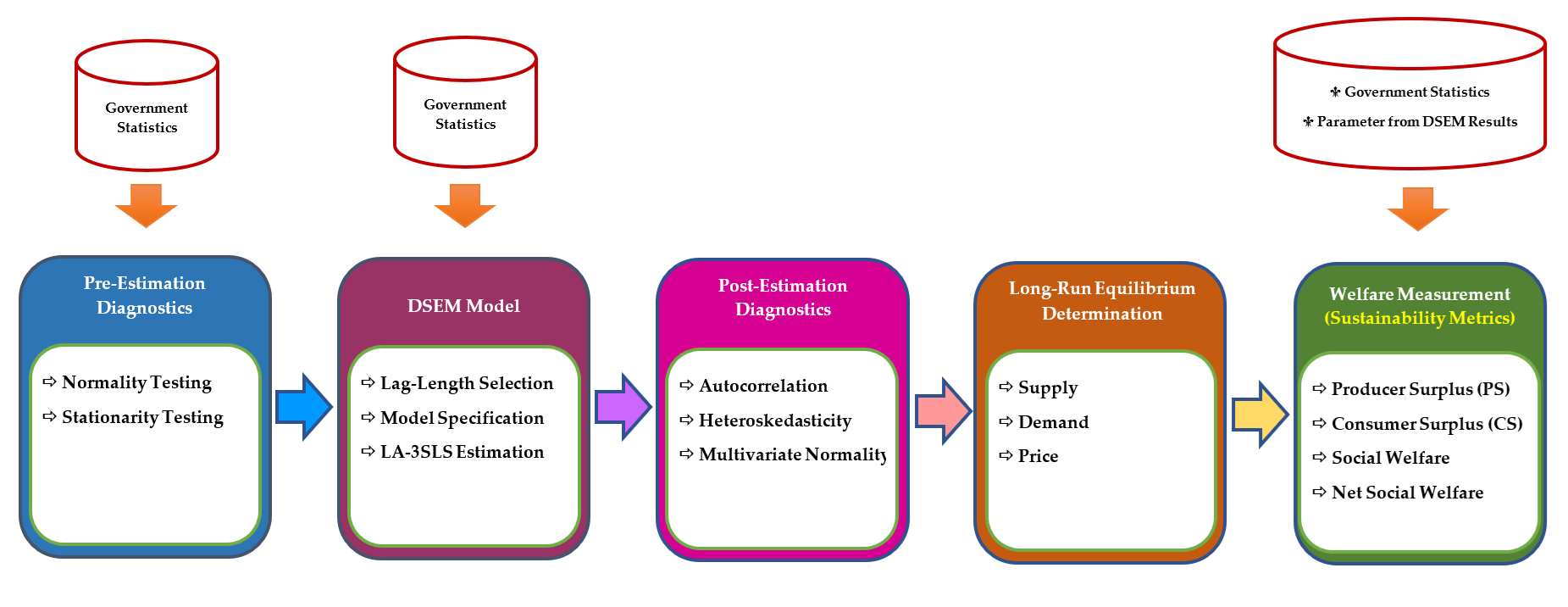
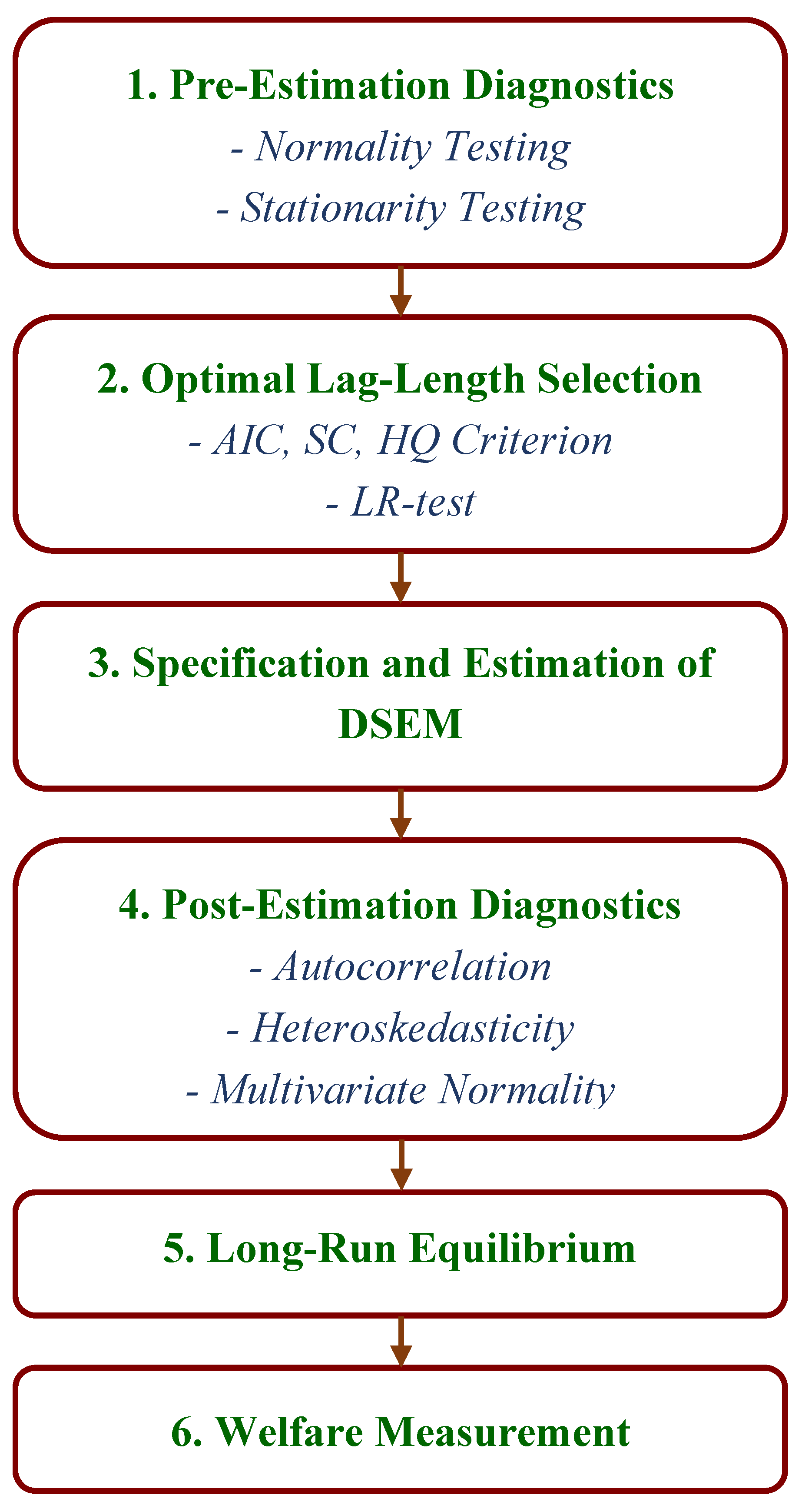
3. Materials and Methods

In this section, the principal data sources are described along with an explanation of the econometric framework used in evaluating the effects of the Thai cassava price-intervention policy on welfare outcomes. This analysis employs a dynamic econometric approach which allows market changes in both the shorter and longer time frames to be taken into consideration.

3.1. Data Collection

Table 2 summarizes all variables used in the Dynamic Simultaneous Equation Model (DSEM), including their definitions, measurement units, and data sources, which together form the empirical foundation for analyzing the long-run behavior of Thailand’s cassava market. Secondary time-series data for 1981-2024 were obtained from the Office of Agricultural Economics (OAE) [43,72], Department of Internal Trade (DIT) [73], Bank of Thailand (BOT) [74], Thai Tapioca Trade Association (TTTA) [75], and the Secretariat of the Cabinet (SOC) [47], representing reliable and consistent datasets that span more than four decades of structural market developments. All price variables were converted into constant 2023 values using the Consumer Price Index (CPI, 2023 = 100) from the Office of Trade Policy and Strategy (TPSO) [76] to remove inflationary effects and ensure comparability in dynamic welfare computations.

The policy dummy variable was coded as $D_{PIP,t}$ = 1 for years in which the fresh cassava pledging scheme was implemented and $D_{PIP,t}$ = 0 otherwise, including years under the income-guarantee program, which provides direct compensation (direct payments) without altering market-clearing prices, and therefore is not considered a price-intervention instrument. Additional variables, such as harvested area, export prices, competing commodity prices, and the exchange rate, were included to capture key supply-demand determinants and price-transmission channels identified in the agricultural economics literature.

3.2. Data Analysis

The impacts of Thailand’s cassava price-intervention policy are assessed using a dynamic econometric framework that captures short-run and long-run adjustments in supply and demand within a partial-equilibrium context. Analysis of the fresh cassava root pledging scheme considers the policy to work by shifting supply, and thus affecting market behavior. The effects are then measured using a system of structural simultaneous equations, which produce parameter estimates capable of determining the welfare indicators of producer surplus, consumer surplus, and total surplus. These values can be derived from integrating the long-run demand and supply curves. EViews 9 was used for all statistical analyses.

Our analysis has six steps: (i) pre-estimation diagnostics; (ii) optimal lag-length selection; (iii) Dynamic Simultaneous Equation Model (DSEM) specification and estimation; (iv) post-estimation diagnostics; (v) determination of the long-run equilibrium, and finally (vi) welfare measurement. A summary of the procedure can be seen in Figure 1.

In the first of these steps, initial diagnostic checks are carried out, testing both normality and stationarity. The data were demonstrated to follow a normal distribution, and therefore the dataset could be considered suitable for inferential statistical analysis. Stationarity testing helps to avoid irrelevant findings which might occur due to non-stationary time-series processes.

In the next stage, the optimal lag structure is chosen, utilizing AIC, SC, and HQ along with likelihood ratio tests. It is important to make use of accurate lag selection in the lag-augmentation process so that the structural model can retain its internal consistency through the estimation procedure.

Following identification of the lag structure, the DSEM can be specified and subsequently estimated. In this study, the equations in question encompass supply and demand, farm-gate price transmission, chip price and starch price formation, and market-clearing conditions. Endogeneity and cross-equation correlation are covered by the LA-3SLS estimator, which also takes into consideration the existence of non-stationary variables while valid statistical inference can be maintained.

Prior to the construction of long-run equilibrium relationships, the adequacy of the model is verified via post-estimation diagnostic tests which examine serial correlation, heteroskedasticity, and the multivariate normality of the residual vector. It is important to carry out such checks to ensure the parameter estimates employed for long-run analysis are reliable. Should these assumptions be broken, the interpretation of market mechanisms may no longer be valid.

Once the diagnosis of the system is complete, long-run demand and supply interactions under steady-state conditions can be derived using the coefficients estimated from the DSEM, and equilibrium outcomes can then be calculated under both policy and non-policy circumstances using information about these relationships. The producer surplus, consumer surplus, and total surplus can be determined via the integration of inverse demand and inverse supply functions. When fiscal costs are also taken into consideration it is possible to present a thorough overview of net social welfare.

3.3. Pre-Estimation Diagnostics

The current research makes use of the Jarque-Bera statistic to evaluate the distributional properties of the stochastic variables. This approach is able to test for skewness and kurtosis deviations from the normal distribution. For analysis purposes, the null hypothesis holds that the series follows a normal distribution, with zero skewness while the kurtosis value is three. The alternative hypothesis holds that the series distribution is not normal, indicated by skewness and kurtosis values which are not zero and three, respectively. Performance of this diagnostic evaluation allows a data generation process which aligns with the distributional assumptions that are necessary in estimating the required simultaneous equations.

This study uses a dataset comprising time-series observations so the stationarity properties of the different variables must be determined prior to conducting the econometric estimation stage. It is common for time-series variables to demonstrate non-stationary characteristics which might lead to irrelevant regression outcomes and the problem of statistical inference. To prevent this issue, unit root testing was carried out for all variables, thus establishing the respective orders of integration.

To evaluate the stochastic qualities of the series, the Augmented Dickey-Fuller (ADF) test created by Dickey and Fuller [77,78] was employed. The ADF procedure evaluates three alternative specifications of the data-generating process in levels: a random walk without drift, a random walk with drift, and a random walk with drift and a deterministic trend. These specifications are expressed as:

$$∆X_t=\gamma X_t+\sum _{i=1}^p{\delta }_i∆X_{t-1}+{\epsilon }_t$$

(1)

$$∆X_t=\alpha +\gamma X_t+\sum _{i=1}^p{\delta }_i∆X_{t-1}+{\epsilon }_t$$

(2)

$$∆X_t=\alpha +{\beta }_i+\gamma X_t+\sum _{i=1}^p{\delta }_i∆X_{t-1}+{\epsilon }_t$$

(3)

The hypothesis structure is:

• $H_0:\gamma =0$, which indicates the presence of a unit root and therefore non-stationarity
• $H_1:\gamma \ne 0$, which indicates stationarity

Rejection of $H_0$ occurs when the test statistic exceeds the absolute value of the critical value at conventional significance levels. In this case, the variable is considered stationary. Failure to reject $H_0$ suggests that the series remains non-stationary. All ADF tests were conducted prior to model estimation to ensure that the subsequent dynamic and simultaneous-equation analyses yield valid and reliable inferences.

3.4. Determination of the Optimal Lag Length

Following the stationarity assessment in Section 3.3, the next step involved identifying the optimal lag length $p$ for the time-series variables to ensure that the dynamic structure of the data is appropriately represented before specifying the DSEM. The lag structure was determined using three widely recognized information criteria: Akaike’s Information Criterion (AIC), the Schwarz or Bayesian Information Criterion (SC or BIC), and the Hannan-Quinn Criterion (HQ). The use of these criteria allows a balance to be achieved between model fit and parsimony, since complexity is avoided where it is not required.

Lag selection can be made more robust by applying the Likelihood Ratio (LR) test, as suggested by Toda and Yamamoto [70] and Hsiao and Wang [69], whose guidance emphasizes the significance of ensuring the accuracy of lag determination when using dynamic econometric models. DSEM construction, which is described in Section 3.5, makes use of the optimal lag length as determined by these criteria as the key input. The DSEM plays a vital role in long-run parameter estimation and the welfare analysis which follows.

3.5. The Dynamic Simultaneous Equation Model (DSEM)

A system comprising six structural dynamic equations is developed to represent the dynamic interactions which take place in the Thai cassava market. These equations encompass the changes attributable to supply and demand responses, price transmission mechanisms, and market clearing conditions. The Lag-Augmented Three-Stage Least Squares (LA-3SLS) estimator [69] is used to estimate the DSEM. This estimator extends the conventional 3SLS method by incorporating additional lag terms to ensure valid statistical inference in dynamic simultaneous equation systems that may contain non-stationary or cointegrated variables. Through this approach, consistent and efficient estimation of the interdependent relationships among cassava market variables is achieved within a unified structural system.

Following the procedure of Hsiao and Wang [69], and consistent with the lag-augmentation method introduced by Toda and Yamamoto [70], each structural equation is augmented by additional lags up to the maximum integration order ($d_{max}$) beyond the optimal lag length $p$. Lag augmentation is applied to the endogenous variables up to ($p+d_{max}$), whereas exogenous variables are augmented only up to $d_{max}$, or in some cases not augmented, in order to avoid over-parameterization. The coefficients associated with these augmented lagged terms are constrained to zero. This restriction ensures that Wald-type test statistics follow their correct asymptotic distributions, preserving the long-run equilibrium properties of the structural system, and allowing standard chi-square-based hypothesis testing to remain valid without requiring prior cointegration testing. As a result, the simultaneous equation estimator remains efficient even under dynamic and potentially non-stationary conditions.

3.5.1. Supply Equation for Cassava Roots (Farm-Gate Level)

$$Q_{S,t}={\alpha }_1+{\beta }_1{Q}_{S,t-1}+{\beta }_2{P}_{FCR,t-1}+\delta D_{PIP,t}+\sum _{i=1}^k{\beta }_{3i}{Z}_{it}+\sum _{j=2}^{p+d_{max}}{(\phi }_{1j}{Q}_{S,t-j})+{\epsilon }_{1t}$$

(4)

Cassava requires six to twelve months from planting to harvest, which prevents farmers from adjusting current output in response to contemporaneous price movements. Consequently, supply decisions depend on expected prices derived from past information. This feature justifies the use of a dynamic decision-making framework that captures intertemporal adjustments between expected and realized prices. The present study adopts the Cobweb theory originally proposed by Ezekiel [79], consistent with the approaches of previous studies [80,81,82], in which farmers are assumed to form naïve expectations by forecasting future prices based on the price observed in the preceding year.

Equation (4) operationalizes the Cobweb mechanism and represents both short-run and long-run supply responses. The lagged supply term $Q_{S,t-1}$ reflects adaptive production adjustment, while $P_{FCR,t-1}$ captures expected price formation through partial adjustment. The variable $D_{PIP,t}$ is a policy dummy that identifies years during which the fresh cassava pledging scheme was implemented as a price-intervention policy. The vector of exogenous variables $Z_{it}$, defined later in the empirical section, includes harvested area, rainfall, fertilizer prices, labor, and a time trend that serves as a proxy for technological progress.

The additional lagged supply terms $Q_{S,t-j}$ are included solely for lag augmentation. While the coefficients ${\beta }_i$ measure economic effects, the augmented-lag coefficients ${\phi }_{ij}$ serve only statistical purposes within the LA-3SLS estimation and do not carry economic interpretation. This specification ensures valid asymptotic inference when endogenous variables exhibit mixed orders of integration.

3.5.2. Demand Equation for Cassava Roots (Farm-Gate Level)

$$Q_{D,t}={\alpha }_2-{\gamma }_1{P}_{FCR,t}+\sum _{j=1}^{p+d_{max}}{{(\phi }_{2j}{Q}_{D,t-j}+\phi }_{3j}{P}_{FCR,t-j})+{\epsilon }_{2t}$$

(5)

Equation (5) models domestic demand responses to farm-gate price changes. The parameter ${\gamma }_1$ measures the effect of the cassava root farm-gate price on demand and is expected to be negative. Lag-augmented terms for both demand and price variables extend from $t-1$ to $p+d_{max}$, consistent with the lag-augmentation procedure.

3.5.3. Cassava Price Transmission Equation at the Farm-Gate Level

$$\begin{gathered} P_{FCR,t}={\alpha }_3+{\gamma }_2{P}_{WCC,t}+{\gamma }_3{P}_{WST,t} \\ +\sum _{j=1}^{p+d_{max}}{{(\phi }_{4j}{P}_{FCR,t-j}+\phi }_{5j}{P}_{WCC,t-j}+{{\phi }_{6j}P}_{WST,t-j})+{\epsilon }_{3t} \end{gathered}$$

(6)

In Equation (6), $P_{FCR,t}$ is the farm-gate price of fresh cassava roots, $P_{WCC,t}$ is the wholesale cassava chip price, and $P_{WST,t}$ is the wholesale cassava starch price. The coefficients ${\gamma }_2$ and ${\gamma }_3$ capture vertical price pass-through from the wholesale level to the farm-gate level, illustrating how price signals originating in downstream markets affect producers. This equation represents the dynamic pathways through which processing sector and export sector price movements transmit to farmers.

3.5.4. Wholesale Cassava Chips Price Equation

$$P_{WCC,t}={\alpha }_4+{\beta }_3{P}_{ECC,t}+{\beta }_4{P}_{WCN,t}+{\beta }_5{THBUSD}_t+\sum _{j=1}^{p+d_{max}}{(\phi }_{7j}{P}_{WCC,t-j})+{\epsilon }_{4t}$$

(7)

This equation specifies wholesale cassava chip prices ($P_{WCC,t}$) as a function of export prices, competing commodity prices, and the exchange rate. The export price of cassava chips ($P_{ECC,t}$) and wholesale corn price ($P_{WCN,t}$​) capture substitution and competitiveness effects, while the exchange rate (${THBUSD}_t$​) links domestic prices to international markets. A depreciation of the Thai baht increases export competitiveness and tends to raise domestic wholesale prices.

3.5.5. Wholesale Cassava-Starch Price Equation

$$P_{WST,t}={\alpha }_5+{\beta }_6{P}_{EST,t}+{\beta }_7{THBUSD}_t\sum _{j=k+1}^{k+d_{max}}{(\phi }_{8j}{P}_{WST,t-j})+{\epsilon }_{5t}$$

(8)

Equation (8) models wholesale starch prices ($P_{WST,t}$) as a function of its export prices ($P_{EST,t}$​) and the exchange rate (${THBUSD}_t$), indicating that changes in international starch prices transmit to domestic markets.

3.5.6. Market Equilibrium Identity

$$Q_{S,t}=Q_{D,t}$$

(9)

The market-clearing condition equates supply with demand, ensuring internal consistency within the structural system.

3.6. Post-Estimation Diagnostics

Following the estimation of the DSEM using the LA-3SLS procedure, a series of diagnostic checks is required to ensure that the estimated structural parameters satisfy the core econometric assumptions necessary for valid inference. These procedures form an essential component of the data analysis process before deriving the long-run supply and demand equations that support the subsequent welfare analysis. Diagnostic assessments focus on autocorrelation, heteroskedasticity, and the distributional attributes associated with the structural disturbance vector.

Initially, the Portmanteau Q-statistic of Hosking [83] is used to investigate autocorrelation throughout the system. It is typical for DSEMs to include lagged dependent variables along with endogenous regressors, which result in serial dependence in the disturbance terms. This kind of dependence leads to distortion in standard errors, and the instrumental variable estimators may exhibit lowered asymptotic efficiency. Autocorrelation testing should therefore be performed at the onset of the study because subsequent procedures are rendered unreliable under conditions of serial dependence.

Following the assessment of autocorrelation, the Breusch-Pagan-Godfrey test [84,85] is used to determine heteroskedasticity. The process is able to identify the incidence of non-constant error variance arising in individual structural equations. It is crucial to manage heteroskedasticity during instrumental-variable and LA-3SLS estimation because the resulting estimators cannot be considered efficient if the variance-covariance matrix of the disturbances is not correctly specified.

The last stage of the diagnostic process demands assessment of the joint disturbance vector to test for normality. In line with Lütkepohl [86], a multivariate normality test can be applied on the basis of the Cholesky orthogonalization of the estimated covariance matrix. This method accounts for the cross-equation covariance that characterizes simultaneous equation systems and provides a rigorous evaluation of the distributional regularity required for system-wide inference.

Taken together, these diagnostic procedures allow an assessment of whether the residual structure satisfies the assumptions required for valid LA-3SLS estimation. This assessment is essential for establishing the statistical reliability of the empirical results that follow and for ensuring that the estimated structural parameters can be used appropriately in the long-run analysis.

Multicollinearity is not considered a diagnostic concern in instrumental-variable simultaneous equation models because endogenous regressors are replaced by their instrumented fitted values, and estimation relies on cross-equation covariance rather than within-equation correlations. For this reason, conventional ordinary least squares diagnostics such as the variance inflation factor (VIF) are not applicable in this context [87,88].

3.7. Long-Run Equilibrium Determination

After estimating the DSEM using the LA-3SLS estimator, the next step is to derive the long-run structural supply and demand equations that characterize the steady-state equilibrium of Thailand’s cassava market. These long-run expressions form the analytical basis for computing producer surplus (PS), consumer surplus (CS), and total surplus (TS). The additional lagged variables included for lag augmentation are not assigned economic interpretation. They serve a technical role that ensures valid asymptotic inference, consistent with the recommendations of Toda and Yamamoto [70] and Hsiao and Wang [69].

The short-run structural equations for supply and demand are presented in Equations (10) and (11). In these expressions, the quantities supplied and demanded in period $t$ depend on lagged output, expected price, and a set of exogenous variables. Harvested area (${AREA}_t$) and the time trend (${TIME}_t$) are grouped into the vector of exogenous supply shifters ($Z_t$), while the policy dummy for price intervention ($D_{PIP,t}$) is separated from $Z_t$ to identify the policy-induced movement in the supply intercept. The short-run supply equation at the farm-gate level is written as:

$$Q_{S,t}={\alpha }_1+{\beta }_1{Q}_{S,t-1}+{\beta }_2{P}_{t-1}+\delta D_{PIP,t}+{\beta }_{3i}{Z}_t+{\epsilon }_{1t}$$

(10)

where the vector of exogenous supply variables is defined as:

$$Z_{it}={\beta }_{31}{AREA}_t+{\beta }_{32}{TIME}_t$$

(11)

To obtain the long-run structural forms, the steady-state conditions are imposed:

$$P_t=P_{t-1}=P^{\mathrm{*}},Q_{S,t}=Q_{S,t-1}=Q_S^{*},Z_t=Z,E\left[{\epsilon }_{1t}\right]=0$$

(12)

Under these conditions, the long-run supply function becomes:

$$Q_S^{*}={\displaystyle \frac{{\alpha }_1+\delta D_{PIP}+{\beta }_{3}Z+{\beta }_2{P}^{*}}{1-{\beta }_1}}$$

(13)

The corresponding intercept, evaluated at $P^{*}=0$ is:

$$Q_{S,0}^{*}={\displaystyle \frac{{\alpha }_1+\delta D_{PIP}+{\beta }_{3}Z}{1-{\beta }_1}}$$

(14)

This result indicates that the price-intervention policy shifts the long-run supply curve vertically by $\delta /(1-{\beta }_1)$. For welfare computation, the long-run supply equation is expressed in inverse form because integration is performed with respect to quantity. The inverse long-run supply function is:

$$P_S^{*}\left(Q\right)={\displaystyle \frac{(1-{\beta }_1)Q{-(\alpha }_1+\delta D_{PIP}+{\beta }_{3}Z)}{{\beta }_2}}$$

(15)

The short-run structural demand equation is:

$$Q_{D,t}={\alpha }_2-{\gamma }_1{P}_t+{\epsilon }_{2t}$$

(16)

Applying the steady-state conditions yields the long-run demand equation:

$$Q_D^{*}={\alpha }_2-{\gamma }_1{P}^{\mathrm{*}}$$

(17)

and its intercept:

$$Q_{D,0}^{*}={\alpha }_2$$

(18)

The inverse long-run demand function is:

$$P_D^{*}\left(Q\right)={\displaystyle \frac{{\alpha }_2-Q}{{\gamma }_1}}$$

(19)

Market equilibrium is determined by equating the long-run supply and demand equations:

$${\displaystyle \frac{{\alpha }_1+\delta D_{PIP}+{\beta }_{3}Z+{\beta }_2{P}^{*}}{1-{\beta }_1}}={\alpha }_2-{\gamma }_1{P}^{\mathrm{*}}$$

(20)

Solving for the long-run equilibrium price yields:

$$P^{\mathrm{*}}={\displaystyle \frac{{\left(1-{\beta }_1\right)(\alpha }_2-{\alpha }_1-\delta D_{PIP}-{\beta }_{3}Z)}{{\beta }_2+(1-{\beta }_1){\gamma }_1}}$$

(21)

Substituting this expression into the long-run demand equation gives the equilibrium quantity:

$$Q^{*}={\alpha }_2-{\gamma }_1{P}^{\mathrm{*}}$$

(22)

These expressions define the long-run market-clearing point under both policy and non-policy regimes. They also provide the computational foundation for welfare analysis. Producer surplus (PS) is obtained by integrating the inverse supply function $P_S^{*}\left(Q\right)$ over the interval $\left[0,Q^{*}\right]$. Consumer surplus (CS) is computed by integrating the inverse demand function $P_D^{*}\left(Q\right)$ over the same interval. Total surplus, defined as the sum of PS and CS, enables a consistent comparison of welfare outcomes between the intervention scenario with $D_{PIP}=1$ and the non-intervention scenario with $D_{PIP}=0$.

3.8. Welfare Measurement

The welfare analysis in this study follows the classical Marshallian framework [89], where consumer surplus (CS) and producer surplus (PS) are measured as the areas between the demand and supply schedules in price-quantity space. In this setting, the inverse demand function denotes the marginal willingness to pay (MWTP), and the inverse supply function represents the marginal cost (MC) or marginal willingness to accept (WTA) [55,91,92]. Integrating these inverse functions with respect to quantity yields aggregate benefits and costs up to the long-run equilibrium quantity ($Q^{*}$). This foundation supports the welfare assessment of Thailand’s cassava price-intervention policy. Kim [92] further establishes that welfare measures based on inverse demand systems are valid when quantities, rather than prices, serve as the exogenous determinants of equilibrium, a condition characteristic of agricultural markets with slow production adjustments.

In Thailand’s cassava sector, farmers supply fresh roots as the primary output, while processors and industrial users generate a derived demand for cassava as an intermediate input [93]. According to the conceptual framework adapted from Zhao, Mullen and Griffith [94], price-intervention instruments, such as pledging programs and guaranteed minimum prices, raise producer incentives and shift the long-run supply curve outward, increasing total market quantity and lowering the long-run equilibrium price under market-clearing conditions. These adjustments create redistributive welfare effects between producers and buyers.

Producer surplus (PS) is defined using the inverse long-run supply function $P_S^{*}\left(Q\right)$:

$$PS=\underset{0}{\overset{Q^{*}}{\int }}\left[P^{*}-P_S^{*}\left(Q\right)\right]dQ$$

(23)

which can also be written as:

$$PS=P^{*}{Q}^{*}-\underset{0}{\overset{Q^{*}}{\int }}{P}_S^{*}\left(Q\right)dQ$$

(24)

with:

$$P_S^{*}\left(Q\right)={\displaystyle \frac{(1-{\beta }_1)Q{-(\alpha }_1+\delta D_{PIP}+{\beta }_{3}Z)}{{\beta }_2}}$$

(25)

The welfare effect on producers is:

$$∆PS={PS}_1-{PS}_0$$

(26)

Consumer surplus (CS) is computed from the inverse long-run demand function $P_D^{*}\left(Q\right)$:

$$CS=\underset{0}{\overset{Q^{*}}{\int }}\left[{P_D^{*}\left(Q\right)-P}^{*}\right]dQ$$

(27)

which can be expressed as:

$$CS=\underset{0}{\overset{Q^{*}}{\int }}{P}_D^{*}\left(Q\right)dQ-P^{*}{Q}^{*}$$

(28)

where:

$$P_D^{*}\left(Q\right)={\displaystyle \frac{{\alpha }_2-Q}{{\gamma }_1}}$$

(29)

The change in consumer welfare is:

$$∆CS={CS}_1-{CS}_0$$

(30)

Total surplus is:

$$TS=PS+CS$$

(31)

and the welfare effect of intervention is:

$$∆TS=∆PS+∆CS$$

(32)

A positive $∆TS$ indicates a net gain, while a negative value implies a net loss. Although the empirical estimates correspond to an interior equilibrium, the analytical framework also accommodates corner-equilibrium cases.

To incorporate fiscal costs, the analysis introduces $GC$, defined as the total budgetary outlays required for program implementation, including administrative expenses, storage and handling, monitoring, and operational losses. This follows full-cost accounting practices in agricultural policy evaluation [95,96,97]. The net welfare measure is:

$$∆{TS}_{net}=∆PS+∆CS-GC$$

(33)

A positive value indicates that welfare gains exceed government costs, while a negative value indicates a net social loss. This approach is consistent with empirical evaluations of agricultural price-support programs that impose substantial administrative and operational burdens on the public sector [97].

4. Results

This section reports the empirical results obtained from the Dynamic Simultaneous Equation Model (DSEM). The analysis is structured to follow the econometric procedures outlined in Section 3, beginning with pre-estimation diagnostics, the selection of the optimal lag structure, and the estimation of the full dynamic system. The use of post-estimation tests subsequently serves to verify the adequacy of the model and guarantee structural parameter reliability. These validated estimates form the basis for deriving long-run equilibrium relationships and for computing welfare effects under both policy and non-policy settings. The results presented in Sections 4.1-4.7 therefore provide a coherent empirical foundation for assessing the long-term economic implications of Thailand’s cassava price-intervention policy.

4.1. Normality Test Results

The test results of the distributional diagnostics in Table 3 indicate that none of the variables reject the null hypothesis of normality at the 5% level. For example, the variable $Q_{S,t}$ reports a Jarque-Bera statistic of 4.2830 with a probability of 0.1175, while $P_{FCR,t}$ and $P_{WCC,t}$ yield probabilities of 0.6180 and 0.4119, respectively. Since all p-values exceed 0.05, the dataset does not exhibit statistically significant deviations from normality. This conclusion is confirmed by the kurtosis measures. While $P_{FCR,t}$ (2.5714) and $P_{EST,t}$ (2.6030) fall a little below the benchmark threshold of 3, they do not specifically imply heavy-tailed behavior.

Furthermore, the descriptive statistics lend weight to significant market variability elements. For instance, a number of price variables are characterized by broad ranges, such as $P_{WST,t}$ (8,190-18,630 THB per ton) and $P_{WCN,t}$ (6,760-12,380). Such ranges are indicative of large fluctuations within the market conditions. In contrast, the close alignment between the mean and median of variables such as PFCR (mean 1904, median 1901) and $P_{ECC,t}$ (mean 225, median 239) suggests limited skewness. Overall, the results indicate that despite economic volatility, the statistical properties of the dataset remain sufficiently stable to support standard econometric estimation without adjustments for heavy-tailed distributions.

4.2. Stationarity Test Results

The Augmented Dickey-Fuller (ADF) results reported in Table 4 provide clear evidence regarding the integration properties of the variables used in the empirical model. Several key price variables exhibit level stationarity. The cassava farmgate price ($P_{FCR,t}$) rejects the unit root null under both the intercept and the intercept plus trend specifications, with ADF statistics of −3.7882 and −4.5239 that are significant at the 1% level (p-value < 0.01). The wholesale cassava starch price ($P_{WST,t}$) is also stationary in levels, as indicated by ADF values of −4.0580 and −4.5709, both significant at the 1% level. By contrast, most quantity variables and several intermediate and export price series are non-stationary in levels, yet become stationary after first differencing. The supply of cassava roots ($Q_{S,t}$) and the harvested area (${AREA}_t$) do not reject the unit root null in levels. Both variables reject it strongly at first differences, with ADF statistics of −7.7721 and −7.6713 for $Q_{S,t}$ and −6.5125 and −6.4123 for ${AREA}_t$ all with p-values equal to 0.0000. The demand for cassava roots ($Q_{D,t}$) displays an identical pattern and is therefore classified as $I\left(1\right)$.

Similarly, the wholesale cassava chips price ($P_{WCC,t}$), the cassava chips export price ($P_{ECC,t}$), the cassava starch export price ($P_{EST,t}$), and the corn wholesale price ($P_{WCN,t}$) all fail to reject the null hypothesis in levels but reject it decisively after first differencing. Their first-difference ADF statistics fall between −7.52 and −6.13, each statistically significant at the 1% level. The Thai baht per U.S. dollar exchange rate (${THBUSD}_t$) also becomes stationary after differencing, with ADF values of −5.3317 and −5.3021 that confirm an integration order of $I\left(1\right)$. The deterministic trend variable, which captures technical change (${TIME}_t$), and the policy dummy variable ($D_{PIP,t}$) are not subjected to unit root testing because they are non-stochastic regressors, consistent with standard time-series econometric practice as described in Hamilton [98].

Overall, the updated ADF results indicate a mixed order of integration across variables. The coexistence of $I\left(0\right)$ and $I\left(1\right)$ variables support the application of the LA-3SLS estimator in levels. This approach allows valid statistical inference without differencing the variables to address non-stationarity.

4.3. Optimal Lag-Length Results

The results of the lag-order selection are presented in Table 5. To carry out the evaluation, the criteria used, including the Schwarz Criterion (SC), the Hannan-Quinn Criterion (HQ), and the Likelihood Ratio (LR) test, must be econometrically reliable. Since both SC and HQ penalize model complexity to a greater degree than AIC, Lag 1 is identified as the optimal specification. At Lag 1, the minimum values of SC (47.6409) and HQ (47.4252) provide evidence that the inclusion of one lag creates a parsimonious model which retains the ability to capture the underlying structure of the data. Lütkepohl [85] reported a similar conclusion, confirming that SC and HQ typically deliver greater stability in the model selection outcomes when samples are small or moderate in size. The penalty terms are large enough to deter overfitting, which can occur with AIC in samples of this magnitude.

The selection of Lag 1 is supported by the LR statistic, since the value for LR of 80.8698 shows statistical significance at the 5% level when the Lag 1 model is compared to the lag-zero specification. It can be inferred that the addition of a single lag leads to a significant upgrade to the explanatory power of the model, but adding further lags has no statistically significant benefit.

Lag 1 can therefore be considered the most suitable lag length on the basis of evidence drawn from the SC, HQ, and LR tests when the DSEM is to be estimated. The model thus achieves a balance between parsimony and the ability to represent the dynamic relationships within the Thai cassava market. Since this optimal lag length $p$ is 1, the LA-3SLS estimation has a lag-augmentation procedure which serves to extend the endogenous variables as far as ($p+d_{max})$. When $d_{max}=1$, the outcome is a total of 2 lags.

4.4. Estimation Results of the DSEM

Table 6 shows the coefficient estimates from the Dynamic Simultaneous Equation Model (DSEM), revealing strong statistical significance. These coefficients show an excellent fit with the economic theory, and suggest that the LA-3SLS estimator is capable of adequately representing the dynamic structure of the Thai cassava market. The lagged supply variable in the supply equation is shown to be very significant (${\beta }_1$ = 0.536, p < 0.01), which suggests that production levels tend to be quite persistent, as one might anticipate due to the seasonal pattern of production based on biological factors as explained in Section 3. A strong positive influence is also exerted by the lagged farm-gate price, which has its basis in the expected price formation from the cobweb framework (${\beta }_2$ = 3,213.247, p < 0.01). The pledging scheme policy dummy generates a notable upward supply shift ($\delta$ = 1.29×10⁶, p < 0.01), which provides clear evidence to cement its status as an instrument which shifts supply. The observed pattern is reinforced by structural factors, with the area harvested having a powerful influence upon supply (${\beta }_{31}$ = 4.589×10⁶, p < 0.01), while a positive effect is also exerted by the time trend (${\beta }_{32}$ = 69,604.44, p < 0.05), suggesting that technological advances are increasingly influential as time passes. The adjusted R² value is 0.8694, which is indicative of strong explanatory power. The findings fit well with the analytical framework which considers policy intervention to be an instrument that shifts the supply curve outward over the longer term.

The parameter estimates of the demand equation also align well with economic theory. A large negative influence on demand (${\gamma }_1$ = −641.019, p < 0.01) is exerted by contemporaneous farm-gate prices, providing clear evidence of a demand relationship which slopes downward. The value for adjusted R² is 0.8294, which shows that our dynamic demand model is able to accurately account for the derived-demand characteristics associated with the Thai cassava market.

The farm-gate price equation shows evidence of vertical price transmission, whereby wholesale cassava chip prices (${\gamma }_2$ = 0.181, p < 0.01) and wholesale cassava starch prices (${\gamma }_3$ = 0.074, p < 0.01) are significantly transmitted to the farm level. The value for adjusted R² is 0.9013, confirming that international processing markets and the formation of farm-gate prices are closely linked, which would be anticipated when considering that the Thai cassava industry relies heavily upon export markets.

The effects of international markets are reflected in the wholesale chip price equation, with markets for competing commodities also proving highly influential. The export chip prices have a substantial effect upon domestic wholesale prices (${\beta }_3$ = 21.920, p < 0.01), while the price of corn, a similar alternative, also contributes significantly (${\beta }_4$ = 0.212, p < 0.01), reflecting substitution in feed and starch manufacturing. The influence of the exchange rate was also significant (${\beta }_5$= 182.551, p < 0.01), in line with expectations based upon the prominent role played by exports in the Thai economy. The value for the adjusted R² was 0.8944, indicating robust relationships. The pattern for the price equation of wholesale starch was similar, as the key drivers are export starch prices (${\beta }_6$ = 32.405, p < 0.01) and the exchange rate (${\beta }_7$ = 447.825, p < 0.01), resulting in an adjusted R² value of 0.7751.

When applied in each of the equations, the estimated coefficients are shown to be statistically significant, with notable explanatory power in line with the theoretical structural relationships which Section 3.5 describes. These relationships are supported by empirical evidence which establishes the parameter foundation used to calculate the long-run equilibrium conditions and carry out the welfare analysis.

4.5. Diagnostic Test Results

The estimated structural parameters must be valid and the long-run and welfare analyses must be reliable. To accomplish these objectives, a number of diagnostic tests were carried out to assess whether the DSEM disturbance processes would be in line with the basic econometric assumptions which are necessary for consistent statistical inference. The diagnosis concerned autocorrelation, heteroskedasticity, and multivariate normality, with findings discussed below.

4.5.1. Autocorrelation Test Results

Residual autocorrelation was evaluated via the Portmanteau test, performed with a maximum lag of 4, which is greater than the DSEM dynamic order under the LA-3SLS framework ($p+d_{max}=2$). This follows the diagnostic requirement that the testing horizon must be greater than the model’s lag order to ensure adequate power for detecting remaining serial dependence. Using lag 4 thus provides a sufficiently rigorous window for verifying white-noise residual behavior.

The test examines whether the residual vector exhibits temporal dependence, with $H_0$ denoting no autocorrelation. When the p-value exceeds the significance level, $H_0$ cannot be rejected. As shown in Table 7, all p-values for lags 1-4 (0.0526, 0.0681, 0.1263, and 0.2449) exceed the 1% threshold. Consequently, the null hypothesis cannot be rejected at any lag, indicating that the disturbance vector behaves as white noise. This confirms that the dynamic specification of the model adequately captures temporal dependence without leaving systematic autocorrelation in the residuals.

4.5.2. Heteroskedasticity Test Results

Table 8 reports the results of the Breusch-Pagan-Godfrey heteroskedasticity tests across all estimated equations. The null hypothesis ($H_0$) specifies that the residuals show homoskedasticity, meaning that no heteroskedasticity is present, whereas the alternative hypothesis ($H_1$) states that the residuals exhibit heteroskedasticity. In every equation, both the F-statistic and Chi-square statistics yield p-values greater than 0.05, indicating that $H_0$ cannot be rejected. Although Equations 4 and 5 show p-values near the 10 percent level, they remain above the conventional 5 percent threshold. Therefore, there is no statistical evidence of heteroskedasticity in any equation of the dynamic system.

4.5.3. Multivariate Normality Test Results

The multivariate normality assessment provides consistent evidence that the disturbance vector of the DSEM follows a normal distribution. Under the null hypothesis ($H_0$: the residuals are multivariate normally distributed) and the alternative hypothesis ($H_1$: the residuals are not multivariate normally distributed), the skewness and kurtosis tests for all five residual components yield p-values that exceed conventional significance levels. The joint skewness statistic (p = 0.5243) and the joint kurtosis statistic (p = 0.9390) both fail to reject $H_0$. In addition, the Jarque-Bera test confirms this result, with a joint p-value of 0.8602. Taken together, these outcomes indicate that the residuals do not exhibit systematic asymmetry or abnormal tail behavior, thereby supporting the validity of the normality assumption required for reliable econometric inference. Table 9

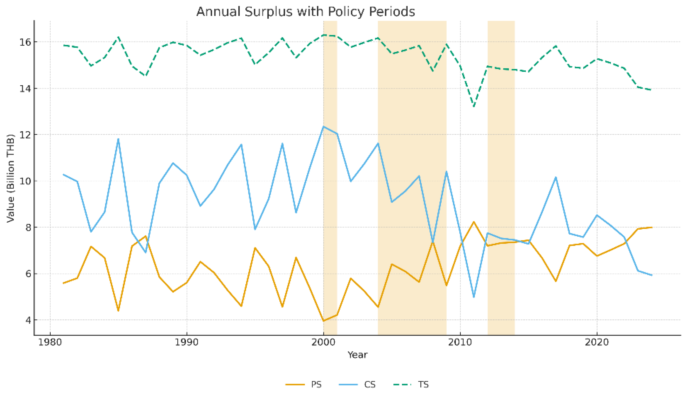
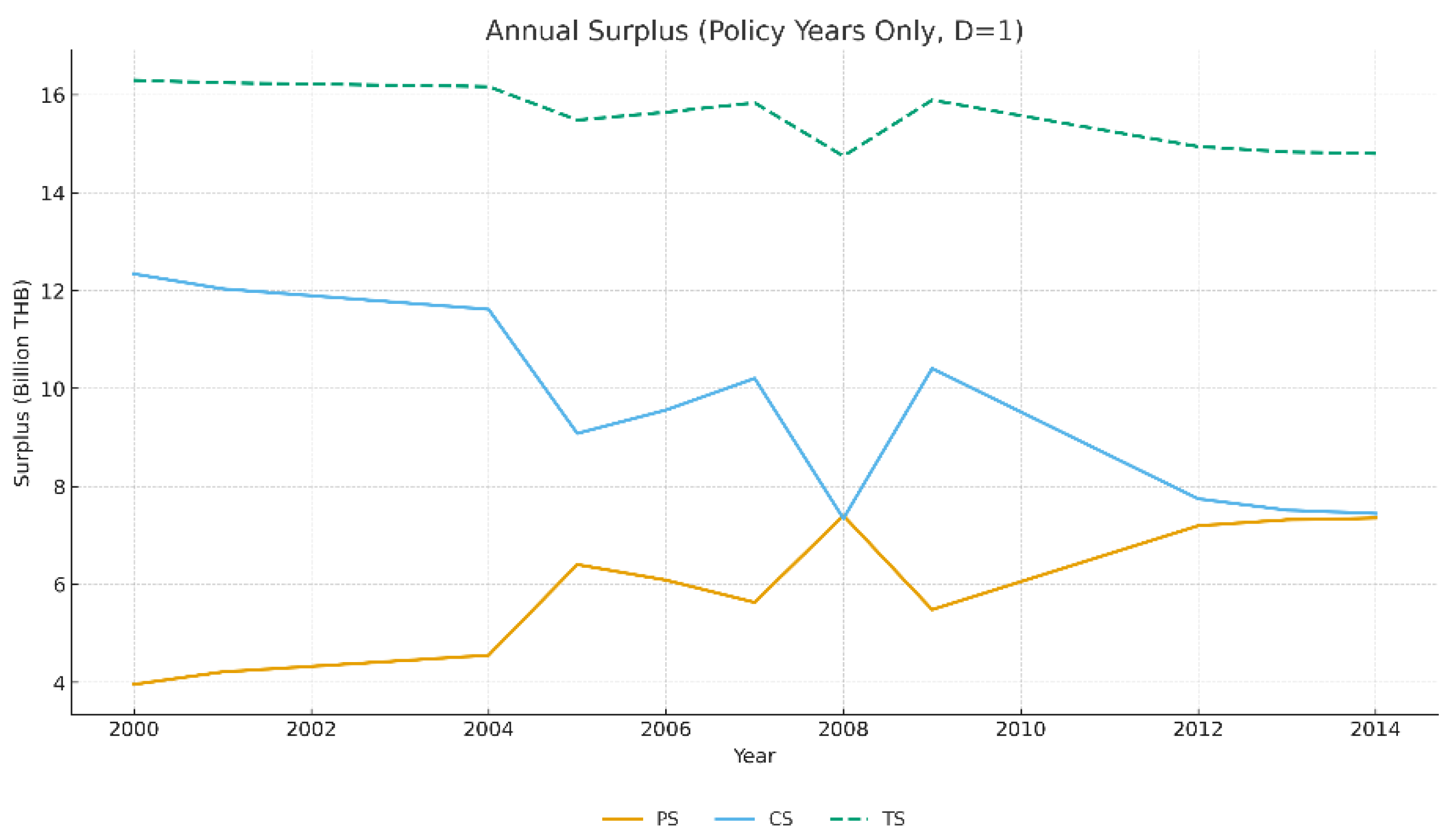
4.6. Welfare Effects of Cassava Price-Intervention Policy

4.6.1. Average Welfare Effects in the Long Term

Based on the long-run structural relationships derived in Section 3.6 and the welfare framework established in Section 3.8, the welfare effects of Thailand’s cassava price-intervention policy were evaluated by comparing producer surplus (PS) and consumer surplus (CS) under two regimes: the non-intervention scenario ($D_{PIP}$ = 0) and the intervention scenario ($D_{PIP}$ = 1) during 1981-2024. The computation relies on the inverse long-run supply function (Equation 25) and inverse long-run demand function (Equation 29), while equilibrium prices and quantities for each regime are obtained from Equations (21) and (22).

To implement these calculations, the analysis requires the estimated structural parameters ${\alpha }_1,{\beta }_1,{\beta }_2,{\beta }_3,\delta$ from the supply equation, and ${\alpha }_2,{\gamma }_1$ from the demand equation, together with the vector of exogenous supply shifters $Z$, defined as the steady-state mean of harvested area and the technological time trend. Using these components, the model derives the market clearing outcomes ($P^{*}$and $Q^{*}$) for both regimes, which are then substituted into the welfare integrals for PS (Equations 23-24) and CS (Equations 27-28).

Table 10 and Table 11 provide the input parameters required for the welfare analysis. Table 10 reports the LA-3SLS structural estimates that define the long-run supply and demand functions and their inverse forms used to compute producer and consumer surplus. Table 11 lists the long-run exogenous supply variables and the policy dummy distinguishing intervention from non-intervention years. These inputs are used to derive the long-run equilibrium and populate the welfare equations, with the resulting welfare outcomes summarized in Table 12.

Table 12 presents the welfare outcomes derived from the long-run equilibrium framework and the welfare-measurement outlined in Sections 3.7-3.8. These results are obtained by integrating the inverse long-run supply and demand functions (Equations 25 and 29) to compute producer surplus (PS) and consumer surplus (CS). The two components are then combined to generate total surplus (TS), as defined in Equation 31.

Under the non-intervention scenario, producers receive 6,602 million THB per year in long-run surplus, whereas consumers obtain 8,760 million THB per year. When the price-intervention policy is applied, PS declines to 6,135 million THB and CS rises to 9,478 million THB per year. These adjustments correspond to $∆PS$ = −467 million THB and $∆CS=718$ million THB per year. The pattern reflects the redistribution implied by the outward shift of the long-run supply curve induced by the pledging scheme. These changes have a size and direction which match the welfare identities of Equations 26 and 30, in which there is a reduction in producer welfare due to distortion of the incentives for production. In contrast, there is an increase in consumer welfare attributable to the effects of policy-driven supply expansion which serve to lower the market clearing price over the longer term.

There is a small increase in total surplus from 15,362 million THB to 15,613 million THB per year, resulting in the value for $∆TS$ = 251 million THB per year. The result matches Equation 32, suggesting that the outcome of the intervention is a small rise in gross economic welfare before considering fiscal costs. Once the government’s budgetary outlays for administering the pledging scheme are incorporated through Equation 33, the net welfare effect becomes negative, as shown by:

$$∆{TS}_{net}=∆PS+∆CS-GC=251-4,811.69=-\mathrm{4,560.69}$$

This result highlights a key implication of the welfare-measurement framework: the policy provides only a negligible increase in total surplus, yet its substantial fiscal burden produces a net social welfare loss of about −4,560.69 million THB per year.

4.6.2. The Dynamics of Long-Term Welfare Effects

The assessment of the long-term welfare effects of Thailand’s cassava price-intervention policy during 1981-2024 was conducted by substituting the estimated structural parameters reported in Table 10, the year-specific values of the exogenous variables, and the policy dummy variables under alternative simulated scenarios into the long-run supply and demand equations evaluated at their steady-state conditions. For the simulations, the policy indicator was defined as $D_{PIP}$ = 0 for years without government price intervention and $D_{PIP}$ = 1 for years in which intervention was implemented.

Figure 2 presents the dynamic evolution of producer surplus (PS), consumer surplus (CS), and total surplus (TS) in Thailand’s cassava market during 1981-2024, with shaded areas indicating years in which price-intervention policies were applied ($D_{PIP}$ = 1). In the short term, the implementation of the fresh cassava pledging scheme produced an immediate rise in PS, together with a corresponding decline in CS. This outcome reflects the pro-producer character of the intervention. When the farm-gate price is held higher than the level at which the market clears, the policy serves to transfer wealth from the consumers to the producers. This redistribution takes place very quickly once the intervention is in place, from which it can be inferred that the cassava supply is highly responsive to government policy.

TS was relatively stable over the longer term, so the pattern observed indicates that the main effect of interventions was to redistribute welfare among market participants instead of making the market more efficient. At the conclusion of the intervention periods, PS showed a tendency to revert to its original levels prior to the intervention. This implies only transient gains for producers, with no sustainable improvement observed in productivity, competitiveness, or the structure of the market. Taken together, the dynamic behavior of the welfare components shows that Thailand’s cassava price-support policies provided short-term protection to producers while delivering limited long-term efficiency gains. The findings reinforce the conclusion that these interventions were transitional measures that redistributed surplus rather than enhancing overall economic performance in the cassava sector.

4.6.3. Welfare Simulation Under Policy and No-Policy Scenarios

The simulation of the long-term welfare effects of Thailand’s cassava price-intervention policy follows the same conceptual procedure as that in Section 4.6.2, although the scenarios differ in the specification of the policy dummy variable. Two scenarios are examined. Scenario 1 represents a situation in which government price intervention is assumed to occur continuously during 1981-2024, with the policy dummy set equal to $D_{PIP}$ = 1 for all years. Conversely, Scenario 2 represents the counterfactual case in which no price intervention is applied at any time during 1981-2024, with the dummy variable fixed at $D_{PIP}$ = 0 throughout the period.

Figure 3 presents the dynamic simulation of long-term welfare under the intervention scenario $D_{PIP}$ = 1. The findings show clearly apparent differences in the development of welfare under the two market scenarios. When continuous government intervention is applied, there is a steady rise in producer surplus, with the opposite trend exhibited by consumer surplus. The pattern is plainly indicative of producer-oriented redistribution effects which result from the cassava-pledging programs. The short-term effect of the policy is to engineer the welfare transfer from consumers to producers as farm-gate prices are held higher than the level at which the market clears, thus providing farm income stability while minimizing price volatility.

However, in the non-intervention scenario shown in Figure 4, the consumer and producer surpluses both fluctuate significantly due to the effects of supply and demand in the market. The pattern shows that the market is able to adjust much more efficiently when policy interventions are absent and thus do not introduce distortions. Over the longer term, the total surplus does not fluctuate greatly in either scenario, but tends to remain slightly lower under conditions of continuous intervention, which suggests that allocative efficiency is lost to a certain extent due to the distortion introduced by the policy. It would appear that farmers might be capable of increasing their producer surplus over time in the absence of state support, thus mitigating the financial burden faced by the government. When the cassava market is permitted to operate freely it is able to reach an equilibrium which ensures allocative efficiency and welfare stability, which is sustainable to the benefit of the economy over the longer term.

5. Discussion

The analysis of welfare in the long run suggests that efficiency and equity are on opposite sides of the balance when price interventions are imposed in the Thai cassava market. While the intervention program delivers income increases to farmers in the short term, the benefits fade rapidly when the intervention is withdrawn, leaving minimal impact upon long-term total surplus. Examination of the incorporation of fiscal costs reveals that a negative net welfare effect is generated by the policy. The government delivers income support on a temporary basis while preparing the ground for ongoing efficiency losses. This pattern shows misalignment with the SDG 1 objective of eliminating poverty, since the emphasis should be placed upon structural reductions in poverty over the long term instead of the short-term income transfers which occur in this scenario. There is also a failure to achieve the SDG 8 objective of decent work and economic growth, since the emphasis of this goal involves long-term productive capacity improvements. The findings appear to concur with the sustainability framework established by Pezzey and Toman [99], in that the redistribution which results from distortionary price policies cannot be considered as sustainable welfare, since it has the effect of damaging efficiency or placing a financial penalty upon future generations.

The dynamic findings add further weight to the evidence report by Anuchitworawong et al. [32], whose work revealed that significant financial burdens resulted from the implementation of the cassava pledging scheme, leading to the accrual of economic rents by intermediaries, while only a minority of farmers actually derived benefits. Their findings in the comparative-static assessment confirmed that inefficiencies arise in the short term. Meanwhile, in this study, the dynamic framework indicated that small distortion tends to occur repeatedly over policy cycles and thus accumulate in the long run, feeding back into the market and affecting long-term behavior and market expectations. Since the total surplus fails to demonstrate any persistent rise in the long term, even though price interventions occur repeatedly, it is clear that the pledging program is not efficient, and furthermore reduces structural competitiveness in the market while persuading participants that ongoing state intervention is likely.

In general, our findings support the need to make adjustments in policy, ceasing the use of repeated price-support interventions and instead employing instruments which are fiscally suitable and more appropriate within the context of the market activity. Farmers can still receive protection from shocks through the use of income-stabilization tools including price insurance or targeted compensatory transfers [18]. Such tools can be applied without the problem of generating artificial demand or encouraging downstream participants to extract rents. Simultaneously, measures which improve productivity, such as managing the soil and water [100], introducing improved crop varieties [101], or utilizing advances in post-harvest technological innovations [102] may provide alternative pathways for boosting producer surplus in the longer term. The market infrastructure could be made stronger by the introduction of farmer registries, effective monitoring systems, and a program for quality certification, since these measures might remove the problem of information asymmetry and eliminate the governance risks which are typically associated with the interventions which have been implemented to date [34].

In considering future studies, it should be noted that three pillars uphold sustainability: economic, social, and environmental factors [49]. It may be possible, therefore, to extends a dynamic framework based on welfare to include environmental indicators [103,104,105], thus enabling a thorough evaluation of long-term policy impacts. It might also be suggested that this dynamic framework could be applied to different agricultural products, or examined in cross-country scenarios, to gain deeper comparative perspectives concerning insights into the longer-term effects of using agricultural price-intervention policies.

6. Conclusions

This research investigated the effects upon long-term economic sustainability of price interventions in the Thai cassava market with the assistance of a Dynamic Simultaneous Equation Model which was estimated via the LA-3SLS procedure. The findings reveal that the main outcome of the pledging scheme is the redistribution of income, instead of the desired improvements in market efficiency. The producers benefit from gains in the short term when the intervention is made, but upon cessation of the intervention, these gains disappear, so the long-term total surplus does not significantly change. If we also take into consideration fiscal expenditures, the net welfare outcome is found to be negative, suggesting that the temporary boost to incomes is more than offset by long-term losses in efficiency.

The structural relationships over the longer term revealed by the dynamic system indicated that when the price intervention is applied repeatedly, supply incentives are altered, leading to a shift in the long-run supply curve. Quantities in the market may rise, but there is no improvement in welfare overall. The results show that equity and efficiency form a trade-off within the mechanism of price support, thereby confirming that pledging schemes are not particularly effective in boosting the competitiveness of markets in the long run.

It can be argued from the results that the Thai cassava industry might better be advanced if direct price controls were rejected in favor of instruments which have the capacity to stabilize farm incomes and support greater market efficiency. Possible solutions might include decoupled income support, counter-cyclical payments, and measures which improve productivity, thus boosting resilience while avoiding the distortion of long-run market signals. This type of approach might be closely aligned with the objectives set out in SDG 1, with is emphasis on structural long-term poverty reduction, as well as SDG 8, which aims for sustainable productivity and a growing economy.

Future studies might seek to expand the current dynamic welfare framework to integrate environmental sustainability indicators. Furthermore, hybrid policy options capable of merging price stabilization and risk management or technological development components might be examined. The use of multi-dimensional sustainability metrics might serve to guide the design and development of policies which can provide welfare protection in the short term while also generating long-term economic resilience.

Appendix A.1

Table A1. Descriptive statistics of variables used in the DSEM.

Variable	N	Mean	Median	Max	Min	SD
$Q_{S,t}$	44	23,226,230	21,070,499	35,094,485	15,254,850	5,837,099
$P_{FCR,t}$*	44	1,904	1,901	3,257	994	527
$P_{WCC,t}$*	44	5,907	5,740	8,580	2,920	1,495
$P_{WST,t}$*	44	13,496	13,475	18,630	8,190	2,593
${AREA}_t$	44	1.29	1.34	1.67	0.99	0.18
${TIME}_t$	44	21.50	21.50	43	0	12.85
$P_{WCN,t}$*	44	9,188	8,915	12,380	6,760	1,552
$P_{ECC,t}$*	44	225	239	386	87	74
$P_{EST,t}$*	44	459	470	732	232	125
${THBUSD}_t$	44	31.60	31.53	44.43	21.82	6.12

* The values of the price variables were converted into constant 2023 values.

Table A1. Descriptive statistics of variables used in the DSEM.

Variable	N	Mean	Median	Max	Min	SD
$Q_{S,t}$	44	23,226,230	21,070,499	35,094,485	15,254,850	5,837,099
$P_{FCR,t}$*	44	1,904	1,901	3,257	994	527
$P_{WCC,t}$*	44	5,907	5,740	8,580	2,920	1,495
$P_{WST,t}$*	44	13,496	13,475	18,630	8,190	2,593
${AREA}_t$	44	1.29	1.34	1.67	0.99	0.18
${TIME}_t$	44	21.50	21.50	43	0	12.85
$P_{WCN,t}$*	44	9,188	8,915	12,380	6,760	1,552
$P_{ECC,t}$*	44	225	239	386	87	74
$P_{EST,t}$*	44	459	470	732	232	125
${THBUSD}_t$	44	31.60	31.53	44.43	21.82	6.12

* The values of the price variables were converted into constant 2023 values.

References

1. Gardner, B.L. The Economics of Agricultural Policies; Macmillan Publishing: New York, NY, USA, 1987; ISBN 0-02-947760-3. [Google Scholar]
2. Anderson, K.; Hayami, Y. The Political Economy of Agricultural Protection: East Asia in International Perspective; Allen & Unwin: Sydney, Australia, 1986. [Google Scholar]
3. Sumner, D.A.; Alston, J.M.; Glauber, J.W. Evolution of the Economics of Agricultural Policy. Am. J. Agric. Econ. 2010, 92, 403–423. [Google Scholar] [CrossRef]
4. Organisation for Economic Co-operation and Development (OECD). The New Rural Paradigm: Policies and Governance. In OECD Rural Policy Reviews; OECD Publishing: Paris, France, 2006. [Google Scholar] [CrossRef]
5. Farm Support and Distortionary Effects; Proceedings of the Expert Meeting on How to Feed the World in 2050; Elbehri, A., Sarris, A., Eds.; FAO: Rome, Italy, 2009; Available online: https://www.fao.org/4/ak542e/ak542e15.pdf (accessed on 3 December 2025).
6. Tyers, R.; Anderson, K. Disarray in World Food Markets: A Quantitative Assessment; Cambridge University Press: Cambridge, UK, 1992. [Google Scholar]
7. Page, T. On the Problem of Achieving Efficiency and Equity, Intergenerationally. Land Econ. 1997, 73, 580–596. [Google Scholar] [CrossRef]
8. Pearce, D. Economics, Equity, and Sustainable Development. Futures 1988, 20, 598–605. [Google Scholar] [CrossRef]
9. European Commission; Directorate-General for Agriculture and Rural Development. Agricultural Policy Perspectives Brief No. 1: The CAP in Perspective – From Market Intervention to Policy Innovation; European Union: Brussels, Belgium, 2011. [Google Scholar]
10. European Commission; Directorate-General for Agriculture and Rural Development. Agricultural Policy Perspectives Brief No. 2: The Future of CAP Direct Payments; European Union: Brussels, Belgium, 2011. [Google Scholar]
11. European Commission; Directorate-General for Agriculture and Rural Development. Agricultural Policy Perspectives Brief No. 3: The Future of CAP Market Measures; European Union: Brussels, Belgium, 2011. [Google Scholar]
12. European Commission; Directorate-General for Agriculture and Rural Development. Agricultural Policy Perspectives Brief No. 4: The Future of Rural Development Policy; European Union: Brussels, Belgium, 2011. [Google Scholar]
13. OECD. Evaluation of Agricultural Policy Reforms in Japan; OECD Publishing: Paris, France, 2009. [Google Scholar] [CrossRef]
14. OECD. Evaluation of Agricultural Policy Reforms in the United States; OECD Publishing: Paris, France, 2011. [Google Scholar] [CrossRef]
15. OECD. Agricultural Policy Monitoring and Evaluation 2025: Making the Most of the Trade and Environment Nexus in Agriculture; OECD Publishing: Paris, France, 2025. [Google Scholar] [CrossRef]
16. European Commission; Directorate-General for Agriculture and Rural Development. Agricultural Policy Perspectives Brief No. 5: Overview of CAP Reform 2014–2020; European Union: Brussels, Belgium, 2013. [Google Scholar]
17. European Commission; Directorate-General for Agriculture and Rural Development. EU-10 and the CAP: 10 Years of Success; European Union: Brussels, Belgium, 2014. [Google Scholar]
18. Food and Agriculture Organization of the United Nations (FAO). Non-Distorting Farm Support to Enhance Global Food Production; FAO: Rome, Italy, 2009. [Google Scholar]
19. Anderson, K.; Valdes, A. Distortions to Agricultural Incentives in Latin America; World Bank: Washington, DC, USA. [CrossRef]
20. Conroy, H.; Rondinone, G.; De Salvo, C.P.; Muñoz, G. Agricultural Policies in Latin America and the Caribbean 2023 2024. [CrossRef]
21. Athukorala, P.; Pham, L.H.; Vo, T.T. Distortions to Agricultural Incentives in Vietnam. of 2): Main Report; Agricultural Distortions Research Project Working Paper No. 26; World Bank: Washington, DC, USA, December 2007. Vol. 1. Available online: http://documents.worldbank.org/curated/en/432701468155378282 (accessed on 5 September 2025).
22. Yan, W.; Huang, K. Determinants of Agricultural Protection in China and the Rest of the World. Asian-Pacific Economic Literature 2018, 32, 64–75. [Google Scholar] [CrossRef]
23. Fane, G.; Warr, P. Distortions to Agricultural Incentives in Indonesia. of 2): Main Report; Agricultural Distortions Working Paper No. 24; World Bank: Washington, DC, USA, 2007. Vol. 1. Available online: https://documents.worldbank.org/curated/en/220901468323377940 (accessed on 5 September 2025).
24. DeBoe, G. Impacts of Agricultural Policies on Productivity and Sustainability Performance in Agriculture: A Literature Review. In OECD Food, Agriculture and Fisheries Papers No. 141; OECD Publishing: Paris, France, 2020. [Google Scholar] [CrossRef]
25. Orden, D.; Cheng, F.; Nguyen, H.; Grote, U.; Thomas, M.; Mullen, K.; Sun, D. Agricultural Producer Support Estimates for Developing Countries: Measurement Issues and Evidence from India, Indonesia, China, and Vietnam. In IFPRI Research Report 152; International Food Policy Research Institute: Washington, DC, USA, 2007. [Google Scholar] [CrossRef]
26. Lyu, J.; Li, X. Effectiveness and Sustainability of Grain Price Support Policies in China. Sustainability 2019, 11, 2478. [Google Scholar] [CrossRef]
27. Li, J.; Liu, W.; Song, Z. Sustainability of the Adjustment Schemes in China’s Grain Price Support Policy—An Empirical Analysis Based on the Partial Equilibrium Model of Wheat. Sustainability 2020, 12, 6447. [Google Scholar] [CrossRef]
28. Ngernklay, P.; et al. Government’s Policy and Measure about Products’ Price Upgrade (in Thai)  . Research and Development Institute, Ramkhamhaeng University; Secretariat of the Senate; Bangkok, Thailand, 2006. Available online: https://prt.parliament.go.th/home (accessed on 24 October 2025).
29. Kohpaiboon, A.; Warr, P.G. Distortions to Agricultural Incentives in Thailand. of 2): Main Report; Agricultural Distortions Working Paper No. 25; World Bank: Washington, DC, USA, 2007. Vol. 1. Available online: http://documents.worldbank.org/curated/en/469601468339594968 (accessed on 5 September 2025).
30. Saiyut, P.; Singhapreecha, C. Political and Economic Impacts of the Price Intervention Policy on Longan (in Thai). Asian J. Appl. Econ. 2013, 14, 103–120. Available online: https://so01.tci-thaijo.org/index.php/AEJ/article/view/10522.
31. Department of Internal Trade. Press Release No. 74: Minister Pichai Orders Action: Major Starch Factories Open Buying Stations for Cassava Farmers to Boost Prices; Ministry of Commerce: Bangkok, Thailand, 29 January 2025; Available online: https://www.dit.go.th/th/news/press-releases/ (accessed on 3 July 2025).
32. Anuchitworawong, C.; Srianunt, N.; Tulayasithpong, S. The Political Economy of the Cassava Market Intervention Measures (in Thai); Thailand Development Research Institute (TDRI); Office of the National Anti-Corruption Commission (NACC): Bangkok, Thailand, 2010. Available online: https://nacc.go.th/categorydetail/2018083118464593/20231101150809 (accessed on 14 May 2025).
33. Amekawa, Y. Rethinking Sustainable Agriculture in Thailand: A Governance Perspective. J. Sustain. Agric. 2010, 34, 389–416. [Google Scholar] [CrossRef]
34. Ruengdet, K.; Wongsurawat, W. The mechanisms of corruption in agricultural price intervention projects: Case studies from Thailand. Soc. Sci. J. 2015, 52, 22–33. [Google Scholar] [CrossRef]
35. Berck, P.; Perloff, J.M. A Dynamic Analysis of Marketing Orders, Voting, and Welfare. Am. J. Agric. Econ. 1985, 67, 487–496. [Google Scholar] [CrossRef]
36. Ciaian, P.; Kancs, D.; Swinnen, J.F.M. Static and Dynamic Distributional Effects of Decoupled Payments: Single Farm Payments in the European Union; LICOS Discussion Paper 207/2008; Available online; Katholieke Universiteit Leuven, LICOS Centre for Institutions and Economic Performance: Leuven, Belgium, 2008. [Google Scholar] [CrossRef]
37. Féménia, F.; Gohin, A. Dynamic Modelling of Agricultural Policies: The Role of Expectation Schemes. Econ. Model. 2011, 28, 1950–1958. [Google Scholar] [CrossRef]
38. Stepanyan, D. From Static to Dynamic-Stochastic Agricultural Partial Equilibrium Models: The Role of Price Expectations and Stockholding. In Working Paper; Humboldt-Universität zu Berlin: Berlin, Germany, 2016. [Google Scholar] [CrossRef]
39. Josling, T. The Historical Evolution of Alternative Metrics for Developing Countries’ Food and Agriculture Policy Assessment. Annu. Rev. Resour. Econ. 2018, 10, 317–334. [Google Scholar] [CrossRef]
40. Food and Agriculture Organization of the United Nations (FAO). Save and Grow: Cassava: A Guide to Sustainable Production Intensification; FAO: Rome, Italy, 2013; Available online: https://www.fao.org/3/i3278e/i3278e.pdf (accessed on 25 June 2025)ISBN 978-92-5-107641-5.
41. International Trade Centre (ITC). Trade Map: Trade Statistics for International Business Development; ITC: Geneva, Switzerland. Available online: https://www.trademap.org (accessed on 15 November 2025).
42. Office of Agricultural Economics (OAE). Thailand Foreign Agricultural Trade Statistics 2024; Centre for Agricultural Information, Ministry of Agriculture and Cooperatives: Bangkok, Thailand, 2025. pp. 1–178. Available online: https://oae.go.th/home/article/393 (accessed on 5 June 2025).
43. Office of Agricultural Economics (OAE). Agricultural Production Data 2024 (in Thai)  . 2024. Available online: https://oae.go.th/home/article/507 (accessed on 5 June 2025).
44. Arthey, T.; Srisompun, O.; Zimmer, Y. Cassava Production and Processing in Thailand: A Value Chain Analysis Commissioned by FAO; FAO: Rome, Italy, 2018; Available online: https://www.researchgate.net/publication/338885781 (accessed on 6 October 2025).
45. Singvejsakul, J.; Chaovanapoonphol, Y.; Limnirankul, B. Modeling the Price Volatility of Cassava Chips in Thailand: Evidence from Bayesian GARCH-X Estimates. Economies 2021, 9, 132. [Google Scholar] [CrossRef]
46. Curran, S.R.; Cooke, A.M. Unexpected Outcomes of Thai Cassava Trade: A Case of Global Complexity and Local Unsustainability. Globalizations 2008, 5, 111–127. [Google Scholar] [CrossRef] [PubMed]
47. The Secretariat of the Cabinet (SOC). Cabinet Resolutions Database (1981–2025); Government of Thailand: Bangkok, Thailand. Available online: https://resolution.soc.go.th/ (accessed on 1 October 2025).
48. Roy, R.; Chan, N.W. An Assessment of Agricultural Sustainability Indicators in Bangladesh: Review and Synthesis. Environmentalist 2012, 32, 99–110. [Google Scholar] [CrossRef]
49. Bathaei, A.; Štreimikienė, D. A Systematic Review of Agricultural Sustainability Indicators. Agriculture 2023, 13, 241. [Google Scholar] [CrossRef]
50. Latruffe, L.; Diazabakana, A.; Bockstaller, C.; Desjeux, Y.; Finn, J.; Kelly, E.; Ryan, M.; Uthes, S. Measurement of Sustainability in Agriculture: A Review of Indicators. Stud. Agric. Econ. 2016, 118, 123–130. [Google Scholar] [CrossRef]
51. Singh, R.K.; Murty, H.R.; Gupta, S.K.; Dikshit, A.K. An Overview of Sustainability Assessment Methodologies. Ecol. Indic. 2012, 15, 281–299. [Google Scholar] [CrossRef]
52. Guth, M.; Smędzik-Ambroży, K.; Czyżewski, B.; Stępień, S. The Economic Sustainability of Farms under Common Agricultural Policy in the European Union Countries. Agriculture 2020, 10, 34. [Google Scholar] [CrossRef]
53. Pannell, D.J.; Glenn, N.A. A Framework for the Economic Evaluation and Selection of Sustainability Indicators in Agriculture. Ecol. Econ. 2000, 33, 135–149. [Google Scholar] [CrossRef]
54. Lynch, J.; Donnellan, T.; Finn, J.A.; Dillon, E.; Ryan, M. Potential Development of Irish Agricultural Sustainability Indicators for Current and Future Policy Evaluation Needs. J. Environ. Manag. 2019, 230, 434–445. [Google Scholar] [CrossRef]
55. Just, R.E.; Hueth, D.L.; Schmitz, A. The Welfare Economics of Public Policy: A Practical Approach to Project and Policy Evaluation; Edward Elgar Publishing: Cheltenham, UK; Northampton, MA, USA, 2004; ISBN 1-84376-688-4. [Google Scholar]
56. Shone, R. An Introduction to Economic Dynamics; Cambridge University Press: Cambridge, UK, 2001; ISBN 0-521-80034-X. [Google Scholar]
57. Shone, R. Economic Dynamics: Phase Diagrams and Their Economic Application, 2nd ed.; Cambridge University Press: Cambridge, UK, 2002; ISBN 978-0-521-81684-7. [Google Scholar]
58. Verdier, V.; Reeling, C. Welfare Effects of Dynamic Matching: An Empirical Analysis. Rev. Econ. Stud. 2022, 89, 1008–1037. [Google Scholar] [CrossRef]
59. Haavelmo, T. The Probability Approach in Econometrics. Econometrica 1943, 11, 1–115. [Google Scholar] [CrossRef]
60. Theil, H. Repeated Least Squares Applied to Complete Equation Systems; Central Planning Bureau: The Hague, Netherlands, 1953. [Google Scholar]
61. Basmann, R.L. A Generalized Classical Method of Linear Estimation of Coefficients in a Structural Equation. Econometrica 1957, 25, 77–83. [Google Scholar] [CrossRef]
62. Sargan, J.D. The Estimation of Economic Relationships Using Instrumental Variables. Econometrica 1958, 26, 393–415. [Google Scholar] [CrossRef]
63. Zellner, A.; Theil, H. Three-Stage Least Squares: Simultaneous Estimation of Simultaneous Equations. Econometrica 1962, 30, 54–78. [Google Scholar] [CrossRef]
64. Greene, W.H. Econometric Analysis, 8th ed.; Pearson/Prentice Hall, 2018; ISBN 978-0134461366. [Google Scholar]
65. Granger, C.W.J.; Newbold, P. Spurious Regressions in Econometrics. J. Econometrics 1974, 2, 111–120. [Google Scholar] [CrossRef]
66. Phillips, P.C.B. Understanding Spurious Regressions in Econometrics. J. Econometrics 1986, 33, 311–340. [Google Scholar] [CrossRef]
67. Pesaran, M.H.; Shin, Y.; Smith, R.J. Bounds Testing Approaches to the Analysis of Level Relationships. J. Appl. Econometrics 2001, 16, 289–326. [Google Scholar] [CrossRef]
68. Hsiao, C. Analysis of Panel Data, 3rd ed.; Cambridge University Press: Cambridge, UK, 2014; ISBN 978-1-109-26091-5. [Google Scholar] [CrossRef]
69. Hsiao, C.; Wang, S. Lag-Augmented Two- and Three-Stage Least Squares Estimators for Integrated Structural Dynamic Models. Econometrics J. 2007, 10, 49–81. [Google Scholar] [CrossRef]
70. Toda, H.Y.; Yamamoto, T. Statistical Inference in Vector Autoregressions with Possibly Integrated Processes. J. Econom. 1995, 66, 225–250. [Google Scholar] [CrossRef]
71. Oliver, M.E.; Mason, C.F.; Finnoff, D. Pipeline Congestion and Basis Differentials. J. Regul. Econ. 2014, 46, 261–291. [Google Scholar] [CrossRef]
72. Office of Agricultural Economics (OAE). Agricultural Product Price Database (in Thai). 2025. Available online: https://oae.go.th/home/article/476 (accessed on 8 June 2025).
73. Department of Internal Trade (DIT). Retail and Wholesale Prices (in Thai). Available online: https://pricelist.dit.go.th/main_price.php?seltime=year (accessed on 25 August 2025).
74. Bank of Thailand (BOT). Average Exchange Rate of Commercial Banks in Bangkok, 1981–2024; Bank of Thailand: Bangkok, Thailand, n.d. Available online: https://www.bot.or.th/en/statistics/financial-market-statistics.html (accessed on 15 July 2025).
75. Thai Tapioca Trade Association (TTTA). Statistics of Cassava Product Exports; TTTA: Thailand. n.d. Available online: https://ttta-tapioca.org (accessed on 19 August 2025).
76. Office of Trade Policy and Strategy (TPSO). Consumer Price Index (CPI) (in Thai); Ministry of Commerce: Thailand. n.d. Available online: https://index.tpso.go.th/cpi (accessed on 20 August 2025).
77. Dickey, D.A.; Fuller, W.A. Distribution of the Estimators for Autoregressive Time Series with a Unit Root. J. Am. Stat. Assoc. 1979, 74, 427–431. [Google Scholar] [CrossRef] [PubMed]
78. Dickey, D.A.; Fuller, W.A. Likelihood Ratio Statistics for Autoregressive Time Series with a Unit Root. Econometrica 1981, 49, 1057–1072. [Google Scholar] [CrossRef]
79. Ezekiel, M. The Cobweb Theorem. Q. J. Econ. 1938, 52, 255–280. [Google Scholar] [CrossRef]
80. Xie, H.; Wang, B. An Empirical Analysis of the Impact of Agricultural Product Price Fluctuations on China’s Grain Yield. Sustainability 2017, 9, 906. [Google Scholar] [CrossRef]
81. Tenaye, A. New Evidence Using a Dynamic Panel Data Approach: Cereal Supply Response in Smallholder Agriculture in Ethiopia. Economies 2020, 8, 61. [Google Scholar] [CrossRef]
82. Guerrini, L.; Anokye, M.; Sackitey, A.L.; Amoah-Mensah, J. Dynamics of a Price Adjustment Model with Distributed Delay. Mathematics 2024, 12, 3220. [Google Scholar] [CrossRef]
83. Hosking, J.R.M. Lagrange-Multiplier Tests of Time-Series Models. J. R. Stat. Soc. Ser. B 1980, 42, 170–181. [Google Scholar] [CrossRef]
84. Breusch, T.S.; Pagan, A.R. A Simple Test for Heteroscedasticity and Random Coefficient Variation. Econometrica 1979, 47, 1287–1294. [Google Scholar] [CrossRef]
85. Godfrey, L.G. Testing Against General Autoregressive and Moving Average Error Models When the Regressors Include Lagged Dependent Variables. Econometrica 1978, 46, 1293–1301. [Google Scholar] [CrossRef]
86. Lütkepohl, H. New Introduction to Multiple Time Series Analysis; Springer: Berlin/Heidelberg, Germany, 2005. [Google Scholar] [CrossRef]
87. Kmenta, J. Elements of Econometrics, 2nd ed.; University of Michigan Press: Ann Arbor, MI, USA, 1997. [Google Scholar]
88. Wooldridge, J.M. Econometric Analysis of Cross Section and Panel Data, 2nd ed.; MIT Press: Cambridge, MA, USA, 2010. [Google Scholar]
89. Marshall, A. Principles of Economics; Macmillan: London, UK, 1890. [Google Scholar]
90. Varian, H.R. Microeconomic Analysis, 3rd ed.; W.W. Norton & Company: New York, NY, USA, 1992. [Google Scholar]
91. Nicholson, W.; Snyder, C. Microeconomic Theory: Basic Principles and Extensions, 11th ed.; Cengage Learning: Boston, MA, USA, 2012. [Google Scholar]
92. Kim, H.Y. Inverse Demand Systems and Welfare Measurement in Quantity Space. South. Econ. J. 1997, 63, 663–679. [Google Scholar] [CrossRef]
93. Muth, R.F. The Derived Demand Curve for a Productive Factor and the Industry Supply Curve. Oxf. Econ. Pap. 1964, 16, 221–234. Available online: https://www.jstor.org/stable/2662270 (accessed on 20 November 2025). [CrossRef]
94. Zhao, X.; Mullen, J.D.; Griffith, G.R. Functional Forms, Exogenous Shifts, and Economic Surplus Changes. Am. J. Agric. Econ. 1997, 79, 1243–1251. [Google Scholar] [CrossRef]
95. Mullen, K.; Orden, D.; Gulati, A. Agricultural Policies in India: Producer Support Estimates 1985–2002; MTID Discussion Paper 82; IFPRI: Washington, DC, USA, 2005. Available online: https://hdl.handle.net/10568/160727 (accessed on 8 July 2025).
96. OECD. OECD’s Producer Support Estimate and Related Indicators: Concepts, Calculations, Interpretation and Use (The PSE Manual); OECD Publishing: Paris, France, 2016; Available online: https://www.oecd.org/... (accessed on 8 July 2025).
97. OECD. The Implementation Costs of Agricultural Policies; OECD Publishing: Paris, France, 2007. [Google Scholar] [CrossRef]
98. Hamilton, J.D. Time Series Analysis; Princeton University Press: Princeton, NJ, USA, 1994. [Google Scholar]
99. Pezzey, J.C.V.; Toman, M.A. The Economics of Sustainability: A Review of Journal Articles; Discussion Paper 02-03; Resources for the Future: Washington, DC, USA, 2002. Available online: https://media.rff.org/documents/RFF-DP-02-03.pdf (accessed on 1 December 2025).
100. Thompson, D.K.; Thepsilvisut, O.; Imorachorn, P.; Boonkaen, S.; Chutimanukul, P.; Somyong, S.; Mhuantong, W.; Ehara, H. Nutrient Management Under Good Agricultural Practices for Sustainable Cassava Production in Northeastern Thailand. Resources 2025, 14, 39. [Google Scholar] [CrossRef]
101. Kongsil, P.; Ceballos, H.; Siriwan, W.; Vuttipongchaikij, S.; Kittipadakul, P.; Phumichai, C.; Wannarat, W.; Kositratana, W.; Vichukit, V.; Sarobol, E.; Rojanaridpiched, C. Cassava Breeding and Cultivation Challenges in Thailand: Past, Present, and Future Perspectives. Plants 2024, 13, 1899. [Google Scholar] [CrossRef]
102. Adejumo, O.; Okoruwa, V.; Abass, A.; Salman, K. Post-Harvest Technology Change in Cassava Processing: A Choice Paradigm. Scientific African 2020, 7, e00276. [Google Scholar] [CrossRef]
103. Lankoski, J.; Nales, E.; Valin, H. Assessing the Impacts of Agricultural Support Policies on the Environment: Economic Analysis, Literature Findings and Synthesis. In OECD Food, Agriculture and Fisheries Papers No. 223; OECD Publishing: Paris, France, 2025. [Google Scholar] [CrossRef]
104. Streimikis, J.; Baležentis, T. Agricultural Sustainability Assessment Framework Integrating Sustainable Development Goals and Interlinked Priorities of Environmental, Climate and Agriculture Policies. Sustainable Development 2020, 28, 1702–1712. [Google Scholar] [CrossRef]
105. Lankoski, J.; Thiem, A. Linkages between Agricultural Policies, Productivity and Environmental Sustainability. Ecol. Econ. 2020, 178, 106809. [Google Scholar] [CrossRef]
Figure 1. Dynamic welfare analysis workflow.
Preprints 190039 g001
Figure 2. Welfare surpluses in the Thai cassava market; the shaded sections indicate policy periods (1981-2024).
Preprints 190039 g002
Figure 3. Annual welfare surpluses in the Thai cassava market when the continuous government price-intervention policy scenario is in place ( D P I P = 1), 1981-2024.
Preprints 190039 g003
Figure 4. Annual welfare surpluses in the Thai cassava market when the non-intervention policy scenario is in place ( D P I P = 0), 1981-2024.
Preprints 190039 g004