
Submitted:
17 December 2025
Posted:
17 December 2025
You are already at the latest version
Abstract
The main aim in this paper is to present a simplified (temperature-dependent) version of the quantum statistical model for computing the equation of state of electrons in materials. For this purpose, the Englert-Schwinger approximation scheme within the quantum statistical model is extended to finite temperatures. This procedure leads to a modified Thomas-Fermi-Dirac model. Schwinger and co-workers had originally demonstrated this procedure for the case of zero-temperature, and applied it to compute the electronic properties of cold free atoms. In this paper, a new algorithm is developed to solve the modified Thomas-Fermi-Dirac model, and the numerical results obtained for Cu and Al are compared with those of the exact quantum statistical model. Good agreement is found particularly for thermal component of electron equation of state. The present approach, at much less efforts, would be useful in high-energy-density physics as thermal component of electron properties alone are needed in equation of state theory. Derivation of explicit expressions of different contributions (viz. kinetic, gradient, exchange and exchange-correlation terms) to the free energy functional, its stationary property, finite-temperature corrections to energy of strongly bound electrons, and (iv) details of the new algorithm are provided in the Appendix.
Keywords:
quantum statistical model
; Thomas Fermi Dirac model
; equation of state
; thermodynamic functions
; virial theorem
; Newton’s method
1. Introduction
Orbital-free density functional theories of electronic structure provide the simplest way for determining the electron-components of thermodynamic properties of materials [1]. The Thomas-Fermi (TF) model with its finite-temperature generalization [2], together with the spherical atomic cell concept, is the workhorse for computing electron-properties of hot dense matter [3,4]. The excellent compilation of approximate solutions of TF equation [5] shows the need for efficient and accurate numerical methods in this field. Addition of the quantum mechanical exchange correction to the TF model leads to Thomas-Fermi-Dirac (TFD) model [6], while the Thomas-Fermi-Dirac-Weizsäcker (TFDW) model, also known as quantum statistical model (QSM), is obtained when electron-density gradient corrections to kinetic energy are also accounted [7]. Numerical computations of electron-component of equation of state (EOS) using the QSM is somewhat involved [8,9]. Moreover, there is no scaling of thermodynamic properties with atomic (Z) and mass (A) numbers [10,11]. Therefore, it would be valuable to have improvements to the TF model, with the addition of electron exchange-correlation and gradient effects, however, at less computational efforts.
In a seminal work, Schwinger showed [12] that bound electron contribution to the energy of a cold free atom within the TF model is divergent, and the addition of the correct component yields the leading correction, proportional to , to TF-energy, which scales as . All energies quoted here are in atomic unit (where e is the electron charge and is the Bohr radius ). He also showed [13] that a second correction, which arises from the gradient of electron density in the atom (as in QSM) is very accurately expressed as two by ninth (2/9) of the exchange correction (which scales as . Of course, the energy of strongly bound electrons has to be corrected in this procedure. An important step in this work is to use TF-density to compute the magnitude of gradient contribution. This is a very plausible assumption as the gradient contribution is only the first quantum correction ( is the reduced Planck’s constant) to TF-energy. So this contribution may be accounted as an accurate correction term. More elaborately, Englert and Schwinger [14] demonstrated that a new energy functional (hereafter referred as Englert-Schwinger (ES) functional) could be introduced, in terms of pseudo electron density and electrostatic potential. Then, the contribution of the gradient term is found expressible as (2/9) of exchange contribution plus the correction. Their computations of electron properties of cold isolated atom showed significant improvements over the results of TF model. In fact, their results of atomic biding energies differ from the corresponding results of Hartree-Fock method by about 1.1 percent (for ) and 0.1 percent for . The new model was also applied in EOS studies to compute (the zero-temperature) pressure of Al and Cu, in compressed volume states, and the results showed good agreement with those of detailed QSM [15].
The present paper is an extension of ES model to finite temperatures, and is motivated by their comment [14] on QSM proper: ’The resulting forth order differential equation for (electrostatic potential) V in QSM is too complicated, and there is the danger of taking too seriously the initial terms of an infinite series of quantum corrections’ (below Eq.3 in page-23 ). So, a relation between the electron density gradient and exchange contributions to free energy functional (at finite temperature) is established first in this paper. This is done without resorting to the properties of TF-density, as was done earlier by Englert and Schwinger. The proportionality factors between the two components are (2/9) and (3/9) in the zero-temperature and high-temperature limits, respectively. A temperature-dependent correction to the energy of strongly bound electons also arises. Thus, the approximation procedure yields a modified Thomas-Fermi-Dirac (mTFD) model, which incorporates the density gradient component accurately. Additionally, the exchange-correlation term is explicitly accounted in the present paper. Then, a new method to solve the mTFD model is presented, which is an extension of a recently developed algorithm for solving the TF model [16]. The algorithms make use of very accurate rational function approximations of Fermi-Dirac integrals [17].
The paper is organized as follows. The relevant formulas related to the QSM are collected in Section 2. The relation between the density-gradient and exchange components, leading to the finite-temperature mTFD model, is derived in Section 3. Thermodynamic functions and virial theorem are discussed in Section 4. The Newton-Ralphson algorithm to solve the mTFD equation is outlined in Section 5, and numerical results and their comparisons are provided in Section 6. Finally, a summary of the work is provided in Section 7. To make the paper totally self-contained, derivation of the various terms in the QSM functional are provided in sections Section 8.1 (kinetic energy term), Section 8.2 (density-gradient term), Section 8.3 (exchange term) , Section 8.4 (exchange-correlation-free-energy) of the Appendix. In addition, the stationary property of the functional, around its minimum, is proved in Section 8.5. The finite-temperature corrections to energy of strongly bound electrons is obtained in Section 8.6, and details of the algorithm is provided in Section 8.7 .
2. Quantum Statistical Model
Mermin [18] extended the Hohenberg-Kohn theorem by showing that, for given temperature and chemical potential , there exists a unique functional of electron density such that is a minimum, where U is an external potential energy per electron. At the minimum, equals the thermodynamic grand potential and is the equilibrium density in presence of U. The explicit form of is not provided by the theorem. The QSM starts with an assumed form for in the atomic cell. This functional of n, for the specific Coulomb case , is expressed as [9,10]
The corresponding has a minimum is proved in the Appendix (see Section 8.5 ). In the above expression, the volume integrals are over the atomic cell of radius R. The last two terms represent electron potential energy from the nuclear charge at the center of the cell, and self repulsive energy of electrons, respectively. Note that e is the magnitude of electron charge and so that is the attractive component of electrostatic energy of one electron at r. The first three terms represent contributions from kinetic energy, density-gradient and exchange-correlation effects of electron states. Although well known, derivation of explicit expressions of these terms, from basics, are provided in different sections of the Appendix. However, for the sake of completeness, these are also briefly discussed below. Thus, the kinetic energy density is
Here, and in what follows, and is the Fermi-Dirac function of order k (see below). Further, is the energy parameter of the model, m is electron mass, is Boltzman’s constant and ℏ is the reduced Planck’s constant . The energy parameter is introduced in electron density as
This follows from the phase-space density . Next, the gradient-correction to kinetic energy is
The symbol ′ in the expression for denotes derivative with respect to the argument. This complicated formula for the coefficient is derived in the Appendix. Using the asymptotic forms and , it is easily verified that and in the appropriate limits.
The exchange-correlation free energy density arises from the requirement of anti-symmetry of the wave function, which includes the effects of Coulomb repulsion of electrons. Computation of this effect requires solution to an interacting many-particle quantum system. Just as in the case of , the expressions obtained within the uniform electron gas (UEG) model are employed here also. Results of extensive quantum Monte Carlo simulations are fitted in terms of electron density and temperature so as to obtain analytical formulas for [19]. Alternately, a mapping of the quantum electron fluid model to the classical fluid model, based on Ornstein-Zernike equations, also provides good results and fits for [20]. All these important points are discussed in the Appendix. However, note that Monte Carlo representations of is of the form
Here, is the average inter-electron distance, defined by . The parameters are complicated (fitted) functions of T and n (see Appendix for explicit expressions of the parameters ).
Finally, note that the pure exchange term is given by
which is also derived in the Appendix. This is a part of , but it is based only on free-electron wave functions. However, for any finite temperature T, electrons become fully degenerate as , and hence in that limit.
The Fermi-Dirac functions, occurring in different expressions, are defined as
These satisfy the recursion relation (where the symbol ′ denotes derivative). This formula readily follows by differentiating the second representation given above.
Note that the energy parameter in the free gas model is where as it is in the TF model. The chemical potential is ( which is also known as Fermi-energy at zero-temperature) and the electrostatic potential energy per electron. The chemical potential in each of the models is determined via the normalization condition with appropriate energy parameter in the density . In QSM or TFD models, is to be determined via minimizing the functional over the local density (Mermin’s theorem quoted above). The minimization is to be done under the constraint , and enters the models as Lagrange multiplier. In all cases, and are related via the Fermi-Dirac function as given by , and the phase space density is .
The condition that the functional derivative of with respect to is zero ( is the Langrange multiplier) yields the Euler-Lagrange equation, to determin in QSM, as
Here, the electrostatic potential V is defined as
so that is the potential energy per electron. Of course, V satisfies the Poisson’s equation and boundary conditions
While the first boundary condition imposes the nuclear charge, the last one mimics the effect of the surrounding medium. The atomic cell is electrically neutral. Since is expressed as functions of , use of the expression reduces Eq.(6) to
The derivative term is an effective potential energy per electron, and it needs to be computed numerically using Eq.(4). Extensive comparison of this effective potential energy, using different approximations to , has been done [21] because of its use in average atom models.
The energy parameter for the TF model follows on neglecting the exchange-correlation and gradient terms. However, the non-linear equation for , viz.
is to be solved in the TFD model [22], as it accounts only for exchange effects. This follows from where the expression is used . This way of solving the TFD model [22], together with the Poisson’s equation for V, is much simpler than the original method due to Cowan and Askin [6]. In lieu of Eq.(2), these authors used a generalized form of TF phase-space distribution function, viz. , where is the momentum-dependent exchange energy. While the TF and TFD models leads to divergence of as , solution of full equation (9) in QSM is known [9,10] to provide a finite value of due to the occurrence of derivative terms in it. Use of Poisson’s equation reduces Eq.(9) to a highly non-linear fourth order differential equation.
By deriving the relation , via using the TF approximation for , and hence , Schwinger simplified the QSM in the T limit. But he found that is divergent because of the use of TF-density in the procedure. However, Schwinger argued that can be omitted together with the substitution of the correct energy of strongly bound electrons in place of the wrong TF-energy of these electrons. He had already obtained the correction term that is needed to remedy the latter defect as . Thus, according to Schwinger, is the non-divergent part of the gradient term that should be used in the QSM functional. This development is quite important because the contribution of the gradient term to thermodynamic properties is relatively small, particularly for temperatures where electron contribution to thermal energy and pressure are significant. Furthermore, the the gradient term is only the leading quantum correction to the semi-classical (TF model) free energy functional (see also Section 8.2). Lastly, it reduces the order of the non-linear differential equation of the model from four to two. Schwinger’s approximation scheme for finite temperatures is explored next.
3. Englert-Schwinger Functional
A relation between gradient and exchange terms is obtained below following the method of Schwinger for zero-temperature [13]. The starting point in the derivation is that the Poisson’s equation for V is also expressed as , where represents the parts in Eq.(9) due to gradient and exchange-correlation effects (see also third para in Section 8.5). Now, on multiplying this equation with , where , and integrating over the atomic cell leads to
where . Next, the term in the integral on the left is written as
where the symbol ′ denotes derivative with . Conversion of the divergence term to surface integrals yields
The surface term is zero at R as vanishes there. But it tends to a finite limit at the origin as . Note that n, and hence , are finite at the origin in QSM. But, this term at is to be ignored together with the replacement of free energy of strongly bound electrons from a quantum mechanical model (see Eq.(13) given below). Now, noting that , the term proportional to is expressed as . Thus, also using the result , the relation in Eq.(11) reduces to
Here, and . The expression in Eq.(12) is a generalization of Schwinger’s relation, between gradient and exchange terms at zero-temperature. The correction term involving vanishes if TF approximation is used for n or , and is neglected hereafter. The parameter tends to (-3/4) and (-1/2) in the limits and , respectively. But reduces to and in these limits. So, it is clear that the proportionality factors between and terms are (2/9) and (3/9) in the two limits. Thus, the Englert-Schwinger functional is obtained (in the limits of zero and high temperature) by using , in lieu of with the definition . The constant takes values (2/9) and (3/9) in the limits and , respectively. Since the range of these limits is very small, all computations reported in this paper employed the geometric average value . The resulting free energy functional is a modified form of TFD functional (denoted as mTFD), the modification being the addition of and the exchange-correlation component. The functional in mTFD is given by
Here, is the correction to energy of strongly bound electrons within a radius . It refers only to kinetic and electrostatic energies (i.e. TF model) because the wrong contribution from gradient term is already omitted. Further, quantum Monte Carlo simulations accurately model the exchange-correlation term in the free energy functional. The quantity is taken as correction in energy as it is computed by conserving the number of states within . As mentioned earlier, equals at zero-temperature when all bound states are considered. It is computed in the Appendix for finite-temperature (see Section 8.6). The scaled factor verses scaled temperature parameter , for the lowest 10 bound states, is shown in Figure 1. The magnitude of the hump in the figure decreases, and the asymptotic value approaches 0.5, if more levels are considered. The symbols in this figure depict the fit function ( with error ) for the correction factor. The difference in the occupation probability of these levels versus (see the inset figure) is less than 1 percent in the entire range of temperature.
The energy parameter obeys the equation . For the sake of compact notation, a combined fenergy density is introduced here. While represents a part of the gradient term, the second is for exchange-correlation contribution. The first term is explicitly evaluated as . Since electron density , Poisson’s equation for V, written in terms of the TF function , is
where . The independent variable is and . Boundary conditions on are reduced to and . After solving the Eq.(14), the chemical potential is obtained as because of the normalization .
4. Thermodynamic Functions
Derivations of the thermodynamic functions within the TF model [3,16] are extended due to the presence of modified-exchange term (representing the density-gradient effects) and exchange-correlation term. Electron pressure is obtained using the definition and Eq.(13). In this step T and are kept constant, where the subscript denotes cell-boundary. Using the relation for derivative with spherical cell-volume, it readily follows that pressure is given by . Last term arises from . Also, note the result . Substitution of free energy densities shows that the terms and cancel out, so that P is expressed as
Note that is evaluated as , where . Accurate approximations exists [23] for the integral term involving .
The potential energy (per cell) of electrons is where is the electrostatic potential due to electrons. This is the same as , so potential energy is given by
On integrating the TF equation [see Eq.(14)], it is found that equals . Similarly, multiplying the TF equation with x and integrating shows that the second integral equals . Thus, is obtained as
The last integral needs to be computed after obtaining the solution and
Kinetic energy of electrons in the cell is expressed in the integral
The phase space density provides this expression. One integration by parts, and the equation for yields
The TF equation [see Eq.(14)] shows that . Then, is obtained as
To use this expression, the last integral also needs to be done numerically. More importantly, Eq.(17) together with Eq.(16) show that
With out the last integral term (see also Eq.(15)), this equation provides the virial theorem within TF model. Now, one integration by parts provides the result
The result is used here. The three expressions in Eq.(15), Eq.(18) and Eq.(19) yield the virial theorem in mTFD model, viz.
The same relation is found [10] in the original QSM because Eq.(18) is also valid there. In the zero-temperature limit, . Then the virial theorem is reduced to . Feynman et al has argued that the last relation is valid in general [2]. It is noted that Cowan et al have used the same for finite temperatures as well [6].
It is necessary to obtain total energy of electrons using the relation . The density profile is kept constant so as to avoid any contribution due to its variation. Multiplication of Eq.(13) by and differentiation with yields
Here, the subscript stands for partial derivative with at constant and n. The second and third terms cancel and the last term vanishes. Thus, E reduces to
Substitution of the explicit form for yields
The result is used in the last step. The integral terms reduces to at zero-temperature. A fitted formula for , obtained from liquid state theory [20], is given in the Appendix (see Section 8.4). A fitted function for the correction term for energy of lowest 10 strongly bound states, , is found adequate even for all temperatures (see Figure 1).
Using the phase-space density function , the number of free electrons (with positive energy) is expressed as
Here, is the incomplete Fermi-Dirac integral [24] of order one-half. The positive quantity arises from the condition [22] of positive total energy of an electron, viz. . Note that this energy includes the contributions from gradient and exchange-correlation terms.
5. Numerical Scheme
The numerical scheme needed to solve Eq.(14) is easily obtained via a slight modification of the recently proposed algorithm [16] for the TF model. First of all, it is rewritten as an integral equation
The boundary conditions are incorporated above and the kernel is for and for . Further, obeys the non-linear equation
Here, denotes the effective potential energy (per electron) due to exchange-correlation term. As already pointed out, is to be computed via a finite difference formula. The second term above is . In comparison to the algorithm for TF model [16], the modification required in the present case is just finding the solution of Eq.(24). But this is easily done via Newton’s method.
To use Newton’s method for Eq.(23), guess-solutions and are assumed first. Then, from Eq.(24), it is noted that . Just like in , the symbol ′ on indicates derivative with . The non-linear term in Eq.(23) is approximated via the expansion . This follows from Taylor’s expansion of (using the relation ) around the function . Substitution into Eq.(23) yields the linear integral equation
The known function is given by
If newton’s method converges, the terms involving Q cancel out and the original Eq.(23) for is recovered. Therefore, to simplify algorithm, is approximated as in the in the Q-function. This amounts to modifying the definition of in Eq.(24) with the constant in place of . Once the linear equation is solved to obtain the improved solution , it is necessary to update also. In the numerical computations, it is found that this updating is best achieved via Picad’s iterations of Eq.(24). The linear approximation connecting and is found to slowdown convergence for expanded volume states and very low temperatures.
It is evident from Eq.(24) that as . However, the integral and the source term (see 25 and 27) in the linear Fredholm integral equation (FIE) exist for because and as . So, starting with guess solution , and corresponding , the FIE is solvable employing well known approaches, say, the Nyström’s method [25]. Thereafter, is updated via Picad’s iterations. A few repetitions of this whole procedure, together with the replacements and provide the required solution, if Newton’s method converges. But for the occurrence of Q-function [see Eq.(26)] in lieu of and Picad’s iterations, the algorithm is identical to that for the TF model [16]. Therefore, additional details of the algorithm are provided in Section 8.7 of the Appendix.
After obtaining the converged profiles of and , the integral is needed (see Eq.(15)) for pressure. An accurate numerical fit [23] is available for . For various components of energy, the integrals , and are required (see equations (16) ), (17) and (21). These integrals are evaluated by dividing the interval [0,1] to sub-intervals and using piece-wise quadratic interpolation functions, as done for (see Section 8.7). The same technique is used for and to facilitate the computation of and ionization .
6. Numerical Results
The method described above is now applied to compute thermodynamic properties of Cu and Al. Results of electron pressure for Cu, obtained in this paper, are given in Figure 2. The symbols in this figure denote the results of QSM reported by Perrot [10]. The curves marked 1, 2 and 3 correspond to values 10, 1 and 0.1, respectively, where . The agreement is good at much less computational effort (in comparison to QSM proper), thereby demonstrating that mTFD is an excellent approximation to the detailed QSM. Similar results for electron energy are given in Figure 3 for three values (10, 1 and 0.1) of density ratio . The binding energy of Cu at is subtracted from the computed values of total energy, as done in the results of Perrot [10]. These comparisons show that the main parts of corrections to TF model, due to exchange-correlation and gradient effects are captured in the mTDF model. It extends the arguments of Schwinger [13], that the gradient effects can be accurately treated as an exchange term, to finite temperature cases. Next, the different components of energy (kinetic, gradient-exchange part, exchange-correlation and potential) for Cu for the case are shown in Figure 4.
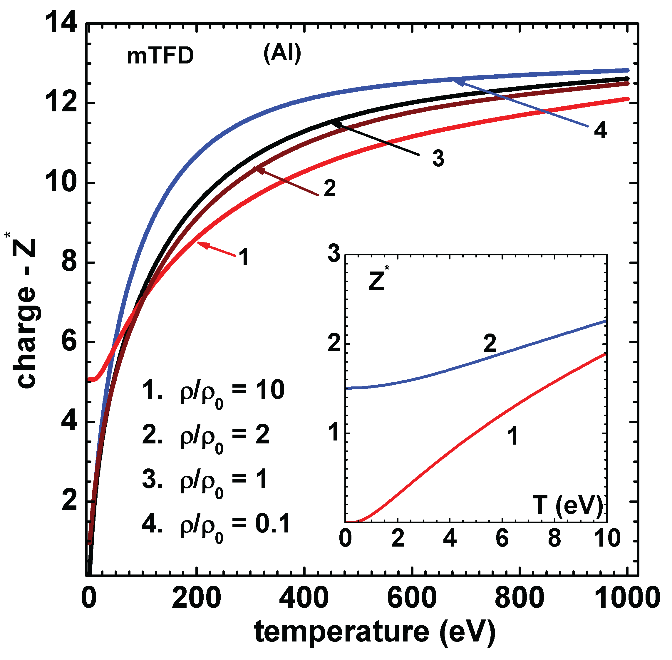
Similar set of results are obtained for Al and are shown in Figure 5 for pressure and Figure 6 for energy. The result for energy corresponding to QSM for the case of 50 eV temperature is from Fromy et al [11], which agree better with those of mTFD. Agreement with results of QSM is again good. Finally, Figure 7 shows the variation of ionization () versus temperature for density rations 10, 2, 1 and 0.1. Note that at 300 K are 5.06 and 0.966 for and 2, respectively. An alternate definition is also used quite often [21]. The values based on this relation and those using Eq.(22 are compared (for ) in the inset figure. All computations leading to the results given above used 20 sub-intervals in [0,1]. Newton’s method converged in less than 10 iterations (criteria ) for all temperatures in the compressed volume states. For expanded volume states and low temperatures ( eV) around 20 iterations were needed.
7. Summary
A simplified version of the QSM for computing the equation of state of electrons in materials is presented. To this end, Englert-Schwinger approximation scheme (at zero-temperature) of QSM is extended to finite temperatures. This procedure leads to a modified Thomas-Fermi-Dirac model (mTFD); the modification being the addition of a term proportional to the exchange free energy in lieu of the gradient term. Of course, the usual exchange-correlation effects are accounted accurately. An efficient numerical algorithm based on Newton’s method to solve the mTFD equation is developed in this paper. The basic idea is to rewrite the mTFD equation as a non-linear Fredholm integral equation and use Newton’s method. Explicit formulas for thermodynamic functions are derived which facilitates computation of pressure and various components of energy of electrons. Numerical results obtained for Cu and Al, using mTFD model, are compared with those based on detailed QSM. Good agreement is found for compressed and expanded volume states. Derivation of explicit expressions of different terms in the free energy functional of QSM are provided in the Appendix. Additionally, the stationary property of QSM is established and temperature-dependent corrections to energy of strongly bound electrons is obtained.
8. Appendix
Key steps in obtaining the expressions (see Eq.(1)) for the four free energy densities , , and are outlined in this Appendix. This includes the empirical formulas for computing the exchange-correlation components, viz, and . These expressions are well known, however, their derivations from first principles are given here for completeness. The stationary property of (finite-temperature) free energy functional of QSM as well as corrections to energy of strongly bound electrons are also discussed.
8.1. Kinetic Free Energy
The starting point is definition of electron density n in the uniform free-gas model (see Eq.(2)) given by where . The thermodynamic definition of chemical potential is . It should be noted that temperature (i.e. ) and volume V are kept unaltered here. Use of the expression gives . This is re-written as . Integration by parts yields . On substituting , integration readily yields . The same expression with general is used in Eq.(1).
An alternate method is to use the Gibbs-Helmholtz equation . The expression for total energy is , where the spatially varying energy parameter is with U denoting an external potential. Integration over yields . Integration by parts (over ) and use of the relation yields
Another integration by parts (over ) shows that
where the definition of n is used. Now, the terms consisting cancel because of the normalization . These steps also show that terms corresponding to TF-model in Eq.(1) follow with the addition of electron-electron potential energy.
8.2. Gradient Energy Density
The approach outlined in this section is along the work of Brack et al [28], however, readers may find that it is more complete and self-contained. The computation of the gradient contribution, to the finite-temperature free energy functional, starts with the definition of density distribution of a single-particle quantum system
where is the Fermi-Dirac occupation probability with denoting the energy of state. The summation in Eq.(28) is over all states (bound and free) and the factor 2 accounts for spin orientations. This definition is applicable to electrons in the atomic cell as they can be ascribed to single-particle states corresponding to a universal (density-temperature-dependent potential) (Mermin’s extension of Homberg-Kohn theorem). Inserting the -function , Eq.(28) is rewritten as
Next, use the Fourier representation (with ) to obtain
Here, a new density , called the Bloch density, is introduced. A nice feature of this expression is that temperature dependent part occurs separately. Now, on writing and integrating by parts yields
The expression is employed above. Using the Fourier transform , above equation reduces to
Here, temperature T appears only in the factor which approaches 1 when . Next, the expression in Eq.(29) is evaluated semi-classically so that the lowest order term is the density in TF model. Higher order terms follow from a series expansion in powers of ℏ.
8.2.1. Bloch Density
To derive the semi-classical approximation, the Bloch-density is written as [29]
where is just a parameter, is the Hamiltonian operator, and it obeys the equation . The last term in Eq.(30) is the trace of the matrix with elements . Now, trace of a matrix is unaltered if its elements are computed with any complete set of orthogonal functions. So, is replaceable with free-particle wave function and the sum is changeable to integration over . This is a crucial point in the development of semi-classical approximations. With these alterations, is expressed as [29]
The factor in front provides the correct number of states in , although is not written explicitly. Denoting , it is easily verified that . Further, as . Then, operating with in H yields [30]
Note that satisfies the equation
and its right-hand-side as . So may be expanded as . Then, it is easily verified that [30]
Solution of these equations give and
Substitution of I in to Eq.(31) provides as [30]
Note that does not contribute to the above as it is proportional to . The constant (see Eq.(2)) is also incorporated. The factor arises due to integration over p over 0 to ∞.
8.2.2. Corrected Density
With the use of Eq.(32), it is now easy to obtain quantum-corrected expressions for density and other thermodynamic quantities. For instance, Eq.(29) readily provides as
The steps leading to Eq.(33) show that the first term 1 inside the square bracket (devoid of and ) must provide the density in TF model (for the potential U), and is given by
Using this definition, is expressed as
Here, primes on denotes derivative with respect to . This generalizes Schwinger’s expression [13] for zero-temperature.
8.2.3. Corrected Free Energy Density
As the free particle entropy is given by , where is the occupation probability, the free energy is . In fact, substitution of and a bit of simplification yield . Note the change of sign in the exponential term. This is convertible to the expression for free energy, given earlier (see Section 8.1) in this appendix, on replacing the sum by integration over , followed by a partial integration. However, the quantum-corrected free energy density is expressed as
Next, introducing the delta function and free particle states to compute the trace (see Eq.(29) ) yield
The first sum is replaced with , which is already obtained in Eq.(34). Two integration by parts converts the logarithmic term to . Then, a Fourier transformation of the cosh term provide
On introducing yields
As done earlier in the case of , the terms devoid of and is identified as proportional to TF-kinetic energy , for the specified potential U, which is given by
Then, is expressed as
The primes on indicates derivative with here also. The chemical potential and energy parameter corresponds to TF model, where as the free energy density is
This form is already derived earlier in Section 8.1 .
8.2.4. QSM-Free Energy Density
For simplifying the expression for , and for developing QSM further, density , including quantum corrections, is re-defined as
The new energy parameter (to be determined) is , with representing a small correction () due to quantum effects. Employing the approximation , TF-free energy density reduces to . Furthermore, it is easily found that as well as . The primes on denote derivatives with and hence the factor . With these changes, Eq.(38) reduces to
The energy parameter in this expression is taken , in lieu of , to the same order of accuracy. The gradient terms in U are now expressed in terms of . Now, Eq.(39) yields , where it is assumed that . In a similar manner . These relations provide
Finally, is given by
The term does not contribute to total free energy as vanishes on the cell boundary and has finite derivative at the origin. Thus the gradient term and the definition of in Eq.(1) follows.
8.3. Exchange Free-Energy
Exchange contribution arises as a pure quantum effect from the symmetry requirement of wave function with respect to exchange of electron’s positions. The two-electron wave function (with spin and position) has to be anti-symmetric on exchange. The electrostatic interaction energy, as given in Eq.(1) (last term), is based on considering elections as particles obeying classical statistics, and the factor (1/2) in front is only because the term inside the integral is for a pair of electrons. In the free-gas model (which is used to compute the exchange effect), the two-electron wave function, with one at and the other at , is where and represent their momenta (), respectively. Box-normalization of a free-particle state is implied here. The classical energy of a pair of electrons now is generalized as . However, the total wave function should be considered as where is the (normalized) anti-symmetric spin component. There is also the possibility of wave function (with symmetric spin component ) where the anti-symmetric space-part is . The factor in front properly normalize . Energy of a pair in the latter state is . Difference of the energy of the two states (in which the spin states are, respectively, and ) is called the exchange energy (per pair)
where and denotes complex conjugate. It is necessary to take so that it decreases the (classical) repulsive energy of a pair, as required for fermions. To go over to quantum statistics in phase space, classical occupation probability (at zero-temperature), viz. is replaced as . Further, the Fermi-Dirac function , for finite-temperature occupation probability at momentum is introduced. Thus, the definition of is changed to , where is the energy parameter in free-gas model. Now, note that the factor [ corresponds to 2 pairs of electrons; two electrons at and other two at . Therefore, the factor [ should be used for the exchange energy per electron. Integration over changes to
which is real as is a function of . Now, the factor corresponds to density of electrons at and at . Therefore, the total exchange energy is [31]
Change of the integral over to integral over the relative co-ordinate shows that . Integration of the angle variables yield . It is possible to simplify the expression for further. To that end, its derivative with is obtained as
This is expressed in terms of using an elegant method [31]. Note that with , . Substitution of this followed by an integration by parts over k yields . Therefore, integration over the angle variable yields where . Integral over r is evaluated as . Therefore, . Using the boundary condition as , integration over yields
where the the definition of is used. Now, it is easily verified that . Thus, substitution of provides the final expression, viz.
The same expression with general , in lieu of , is used in Eq.(1).
8.4. Exchange-Correlation Free-Energy
The formula for exchange free energy derived in the previous section assumes free-electron wave functions. However, effects of electron-electron repulsion (on wave functions), within the uniform electron gas model, is needed in the free energy functional of QSM. The exchange effect when the wave functions also account for repulsive interactions is termed as exchange-correlation free-energy . Quantum ab initio simulations are useful to compute this quantity. These use the standard random sampling techniques, however, the functional that is minimized is based on wave functions obeying symmetry requirements. Alternatively, the techniques based on path-integral approach compute averages like (where denotes n-particle wave function dependent on co-ordinates ) to obtain quantum mechanical partition function and thermodynamic properties.
First of all, note that the (configuration) free energy, of N particles in volume V, due to a inter-particle potential is given by , where denotes N-dimensional configuration integral. This is the definition of free-energy in terms of the partition function . Differentiation by gives where is the distribution function for two-particles separated by r. The pair-distribution function is , which tends to 1 and , is related to as . On changing integration over to and taking the thermodynamic limit yields . Further, integration over gives free energy per electron as . This formula is applicable to the UEG model if , the Coulomb energy, and is obtained incorporating quantum effects. On subtracting the classical interaction energy per particle, viz. , the remaining exchange-correlation free energy per particle is obtained as . Here, is known as the pair correlation function. This is called the coupling-parameter integration for . It is the quantity that is computed via quantum ab initio simulations.
The integration variable is replaceable with inter-particle distance defined as . Now, using , first rewrite free energy as where . As is a functional of , it follows that . Multiplying and dividing by yields and so . A change of integration variable yields . Differentiation with yields the relation . The quantum ab initio simulations generate for a series of thereby determining using the above formula. Using extensive data sets of , generated for the UEG [19], exchange-correlation free energy per electron is fitted as
The parameters are functions of where the Fermi-temperature is defined as . Note that the right-hand-side is the Fermi-energy.
The exchange-correlation energy (per electron) is to be obtained numerically. Similar is the case for the effective potential energy (per electron) .
The approach based on the liquid state theory also provides good results. If and denote the correlation functions for parallel and anti-parallel spin orientations, then . Perrot and Dharma-wardana [20] developed a mapping of the UEG model to a classical two-component fluid model (based on Ornstein-Zernike equation) for computing . Extensive database, as a function of n and T, generated using this method is then converted to fitting formulas for as well as the exchange-correlation energy (provided as supplementary material). In a recent paper, Faussurier [21] reported the formula of Perrot and Dharma-wardana for . To provide this formula, first of all define three functions, viz. , and . Five fitting functions are introduced as
With these parameters, energy per electron is expressed as
Ichimaru et al show that this expression is analytically convertible to the free energy per electron [32]. With the definition of additional functions (see Faussurier’s paper [21] also)
the, free energy (per electron) is expressed as
Note that in denotes natural logarithm. An alternate, but equivalent, fit ( using liquid state theory results) for is provided by Perrot and Dharma-wardana [20].
8.5. Stationary Property of Free Energy
A procedure, introduced by Englert and Schwinger [14], to show the stationary property of is extended to finite temperature in this section. The stationary property is assumed (necessary condition) to derive the Euler-Lagrange equations, but the reverse provides the sufficient condition. Further, this demonstration illustrates Homberg-Kohn-Mermin theorem for the specific functional that is postulated in QSM.
Let the triplet be perturbed as , and , where are first order quantities. It is intended to show that if the triplet are chosen appropriately. As V and U need to obey the Poisson’s equations, with densities n and , respectively, it follows that . Now, Taylor’s expansion of around shows that . Thus, only one of parameters in is independent. Similarly, Taylor’s expansion of together with the relation between and readily yields . Thus, the increment in , in changing from n to , turns out to be .
Using Taylor’s expansion, the incremental change in gradient term is expressed as . Similarly, the exchange-correlation term contributes the incremental change Both these together is expressed as . (The term , originating from exchange and gradient terms, is also made use of in Section 3). Thus, the sum of the changes is . The relation between and is also employed in this step.
Now, let it be assumed that , where corresponds to the -system. This relation is identical to the Euler-Lagrange equation given in Eq.(9), however, the triplet occur in lieu of . Substitution of then yield . The term involving is dropped as it does not contribute to the integral over the atomic cell. This is so because since total charge is the same. The expression for completely cancels with the change in electrostatic interaction energy as shown below. However, Englert and Schwinger [14] chose so that this terms cancels the gradient term. This is readily seen to be possible after two partial integration as surface terms vanish. However, this approach equates an O(1) and O(0) quantities which is undesirable.
The interaction free energy is , as provided by Eq.(1 and Eq.(7). Then, the increment is , where symmetry of with respect to interchange of and is employed. Now, the relation , which follows from the Poisson’s equation for , shows that which cancels . Thus, the sufficient condition, , (i.e. the Euler-Lagrange equation) is shown to vanish the first order derivative terms, and hence, the stationary property of in QSM. No appeal to TF model is needed, as employed in the earlier work (of Englert and Schwinger) for zero-temperature [14].
8.6. Strongly Bound Electrons
The nearly free electron concept embedded in the kinetic energy of QSM is inadequate for strongly bound electrons. For the cold isolated atom, Schwinger [12] re-derived Scott’s correction term , where is the Bohr radius, to TF binding energy [. The correction arises because of inadequate accounting of kinetic and electrostatic energies of strongly bound electrons in TF model. The derivation given below is more complete, and provides the basis for extension to finite-temperatures.
The free energy functional in Eq.(1) should be corrected with the term which amounts to replacing free energy (kinetic and electrostatic) of strongly bound electrons in TF model with a quantum mechanical (QM) expression ( see Section 3 ) . The latter accounts for discrete structure of electron states within a sphere of radius . When minimizing Eq.(1) with respect to density , under the constraint , it is necessary to insist that the number of states within is the same in both (TF and QM) models. Since entropy is directly related to number of states, it may be assumed to be the same in both models. Then, the correction term is expressed in terms of energy difference, viz., where electrons with energy are included in each term in the integral. Here, is a positive number, like binding energy of lowest bound state. The conservation condition of number of states provide the equation to fix the arbitrary value of which is related to . For these electrons, the potential energy is nearly Coulomb, and is (approximately) given by , where is the contribution of electrons outside radius .
In the TF model, the number of these states is where the momentum-integral is restricted by because . This inequality shows that is fixed as , which yields with . Further, it also gives the maximum momentum . These relations, together with the value of the integral , readily give the result where . Here, is twice the ground state binding energy of H in non-relativistic QM [12]. The cumulative number of states via QM model is for the Coulomb potential , where k is an integer (the principal quantum number), and the factor 2 is for spin degeneracy. As this is more than , the parameter should be chosen [12] between k and . Therefore, equals and 3.475 for and 3, respectively, and for large k. Choice of a specific value of k (say, k=1 for the ground state) fixes and hence also and .
Kinetic and electrostatic energy of electrons in TF model is easily obtained as . Values of the integrals and are also used here. As explained earlier (see Section 3), contributions from the gradient and exchange-correlation terms need not be considered. The energy of electrons in k states via QM is . This is so because in the potential , the electron state has energy which should be less than , that is, . The good approximation provides, for the cold free atom, , which is Scott’s correction. Using the semi-classical WKB method of March [27], for computing energy of bound electrons in Coulomb potential, Barnes[26] also derived the same result.
For finite temperature, number of electrons must be computed using the Fermi-Dirac occupation probability . As this probability is required for , where the potential energy dominates, is neglected and is taken as the Coulomb term . Then, the number of electrons and energy in TF model are expressed as and . The temperature-dependent factors (which are normalized to 1 as ) are easily obtained as
Here, . Note that ( within the integrals ), and so approaches 1 as . Further, a very plausible choice (i.e. ten states) shows that so that even for high temperatures. This is also evident from the corresponding quantities of the QM model. These are expressed as and , with the normalized temperature-dependent factors
The factor shows that and are close to 1 even for high values of . For all numerical applications, the fitted function provide accurate results ( error ) for all temperatures (see Figure 1).
8.7. Solution via Nyström’s Method
The Nyström’s method to solve Eq.(25), and the source function in Eq.(27), converts them to a matrix equation [25]. To this end, the integral term and the source function are suitably evaluated by a quadrature formula. In this work, (as well as are approximated using piece-wise quadratic polynomials in the sub-intervals covering [0, 1]. For this purpose, the interval [, 1] is divided in to N (even) sub-intervals defined with (odd) mesh points defined as . This choice of yields more mesh points near where varies more steeply. There are only unknowns to be determined as is known. In the sub-interval (), the unknown function is represented as a quadratic polynomial . The Lagrange polynomials are defined as (for ) so that these are normalized to unity at and pass through others. Similar representation is employed for and . Substitution of into Eq.(25) yields Nyström’s interpolation formula
The weight functions (for ) are given by
For expressing , additional weight functions are defined as
Then, the source term is expressed as
Note that the second sum (with on lower limit), involving , is only over even values of j. The last integral term is obtained by adding up all contributions in the interval , and also using the approximation .
Expressing and expanding near , it is easy to show that . The definition of involving is used here to account for the exchange contribution. Thus, in is approximated by the quadratic polynomial for all computations. This polynomial passes through and and has the correct variation near the origin. The slope is given by
Differentiation of Eq.(23) provides the first equality. Currently available values of and are employed in Newton’s iterations. Furthermore, all the integrals are evaluated using low order (say 6 or 8) Gauss quadrature formula. It is to be noted that the asymptotic term should be subtracted in the integral in Eq.(52) (before applying Gauss quadrature formula) and its contribution added separately. The steps involved in obtaining Eq.(47) are the same as in deriving three-point Simpson’s integration formula. Hence the local truncation error in the method is proportional to . In the collocation rule in Nyström’s method, Eq.(47) is enforced at the discrete set of values , which yields a matrix equation of order for the vector . The coefficient matrix is . The components and those of of the vectors and are and , respectively.
References
- Nikiforov, A. F. ; Novikov, V. G. ; Uvarov, V. B. Quantum-statistical models of hot dense matter: Methods for computation of opacity and equation of state. In Progress in Mathematical Physics, volume 37, Eds: De Monvel, A.B. ; Kaiser, G. Birkhäuser Verlag, Basel, Switzerland, 2005.
- R.P. Feynman, N. Metropolis and E. Teller. Equation of state of elements based on the generalized Fermi-Thomas theory. Phys. Rev. 1949, 75, 1561. [CrossRef]
- Latter, R. Thermal behavior of Thomas-Fermi statistical model of atoms. Phys. Rev. 1955, 99, 1854.
- Shemyakin, O. P. ; Levashov, P. R. ; Obruchkova, L. R. ; Khishchenko, K. V. Thermal contribution to thermodynamic functions in the Thomas-Fermi model. J. Phys. A: Math. Theor. 2010, 43, 335003. [CrossRef]
- Pert, G. J. Approximations for the rapid evaluation of the Thomas-Fermi equation. J. Phys. B: At. Mol. Opt. Phys. 1999, 32, 272. [CrossRef]
- Cowan, R.D; Ashkin, J. Extension of the Thomas-Felllli-Dirac Statistical Theory of the Atom to Finite Temperatures. Phys. Rev. 1957, 105, 144. [CrossRef]
- Kalitkin, N. N. ; Kuz’mina, L. V. Curves of cold compression at high pressures. Sov. Phys. Solid State 1972, 13, 1938.
- Perrot, F. Zero-temperature equation of state of metals in the statistical model with density gradient correction. Physica 1979, A 98, 555. [CrossRef]
- More, R. M. Quantum-statistical model for high-density matter. Phys. Rev. 1979, A 19, 1234. [CrossRef]
- Perrot, F. Gradient correction to the statistical electronic free energy at nonzero temperatures: Application to equation-of-state calculations. Phys. Rev. 1979, A 20, 586. [CrossRef]
- Fromy, P; Deutsch, C and Maynard, G. Thomas-Fermi-like and average atom models for hot dense and hot matter. Physics Plasmas 1996, 3, 714. [CrossRef]
- Schwinger, J. Thomas-Fermi model: The leading correction Phys. Rev. 1980, A 22, 1827.
- Schwinger, J. Thomas-Fermi model: The Second correction Phys. Rev. 1981, A 24, 2353.
- Englert, B. G and Schwinger, J. Thomas-Fermi revisited: The outer regions of the atom Phys. Rev. 1982, A 26, 2622. [CrossRef]
- Venkat Ramana, A. S. and Menon, S. V. G. Application of the Englert–Schwinger model to the equation of state and the fullerene molecule Physica 2011, A 390, 1575. [CrossRef]
- Menon, S. V. G. Analytical Representations of Thermodynamic Functions of Thomas-Fermi Model, Phys of Plasmas 32, (10), 5.0293395, DOI: 10.1063/5.0293395. [CrossRef]
- Antia, H. M. Rational function approximations for Fermi-Dirac integrals. Astrophys. J. Suppl. Series 1993, 84, 101. [CrossRef]
- Mermin, N. D. Thermal Properties of the Inhomogeneous Electron Gas . Phys. Rev. 1965, 137, A 1441. [CrossRef]
- Goth, S; Dornheim, T; Sjostrom, T; Malone, F. D; Foulkes, W. M. C; Bonitz, M. Ab initio Exchane-Correlation free energy of uniform electron gas at warm dense matter conditions. [CrossRef]
- Perrot, F; Darmma-wardana, M. W. C. Spin-polarized electron liquid at arbitrary temperatures: Exchane-Correlation energies, electron-distribution functions, and the state response functions. Phys. Rev. 2000-II, B 62, 16536. [CrossRef]
- Faussurier, G Exchane-Correlation potential at finite temperature. Phys. Plasmas 2025, 32, 072713.
- Szichman, H. Eliezer, S. and Salzmann, D. Calculation of the Moments of the Charge state distribution in hot and dense plasmas using the Thomas-Fermi models J. Quant. Spec. Rad. Trans. 1987, 38, 281. [CrossRef]
- Karasiev, V. V. Chakraborty, D. Trickey, S. B. Improved analytical representation of combinations of Fermi–Dirac integrals for finite-temperature density functional calculations Comp.Phys.Comm. 2015, 192, 114.
- Goano, M. Computation of complete and incomplete Fermi–Dirac integral ACM Transactions on Mathematical Software 19955, 21, 221.
- K. E. Atkinson, The numerical solution of integral equations on the second kind Cambridge University Press, Cambridge. 2009. [CrossRef]
- Barnes, J. F. and Cowan, R. D. Atomic Binding Energies from a Modified Thomas-Fermi-Dirac Theory Phys. Rev. 1963, 132, 236. [CrossRef]
- March, N. H. and Plaskett, J. S. The Relation between the Wentzel-Kramers-Brillouin and the Thomas-Fermi Approximations Proc. R. Soc. Lond. A 1956, A 235, 419. [CrossRef]
- Bartel, J. Brack, M. and Durand, M. Extended Thomas-Fermi Ttheory at finite temperature. Nuclear Physics bf 1985 A 445, 263. [CrossRef]
- Uhlenbeck, G. E. Beth, E. The quantum theory of the non-ideal gas I - Deviations from classical theory. Physica 1936, 3, 729. [CrossRef]
- Landau, L. D. and Lifshitz, E. M. Statistical Physics. In Course of Theoretical Physics, Volume 5, 3rd Edition, Part 1( Revised and Enlarged by Lifshitz, E. M and Pitaevskii, L. P. Translated by Sykes, J. B. and Kerarsley, M. J.) Pergamon Press, Oxford, New York, Beijing 1989.
- Horovitz, B. Thieberger, R. Exchange integral and specific heat of electron gas. Physica 1974, 71, 99. [CrossRef]
- Ichimaru, S; Iyetomi, H; Tanaka, S. Statistical physics of dense plasmas: Thermodynamics, transport coefficients and dynamic correlations. Phys. Rep. 1987, 149, 91. [CrossRef]
Figure 1.
Correction factor to TF-energy of lowest 10 strongly bound states versus scaled temperature , where . Symbols depict the fit function . The inset figure shows the difference in occupation probability (of TF and QM models) of same 10 states versus scaled temperature.
Figure 1.
Correction factor to TF-energy of lowest 10 strongly bound states versus scaled temperature , where . Symbols depict the fit function . The inset figure shows the difference in occupation probability (of TF and QM models) of same 10 states versus scaled temperature.
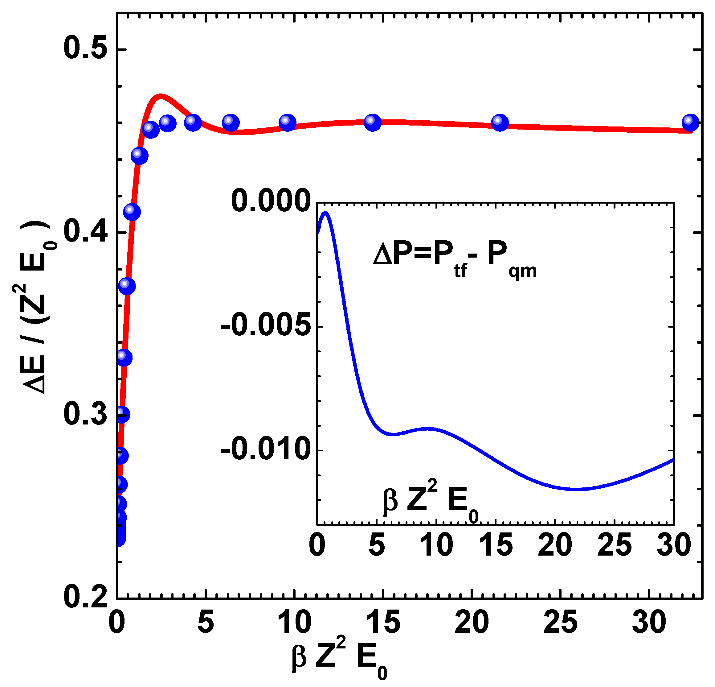
Figure 2.
Pressure (100 GPa) versus temperature (eV) of Cu using mTFD model of this paper (lines) and finite-temperature-QSM (symbols) [10]. Curves marked 1, 2 and 3, respectively, correspond to , 1, and 0.1 , where .
Figure 2.
Pressure (100 GPa) versus temperature (eV) of Cu using mTFD model of this paper (lines) and finite-temperature-QSM (symbols) [10]. Curves marked 1, 2 and 3, respectively, correspond to , 1, and 0.1 , where .
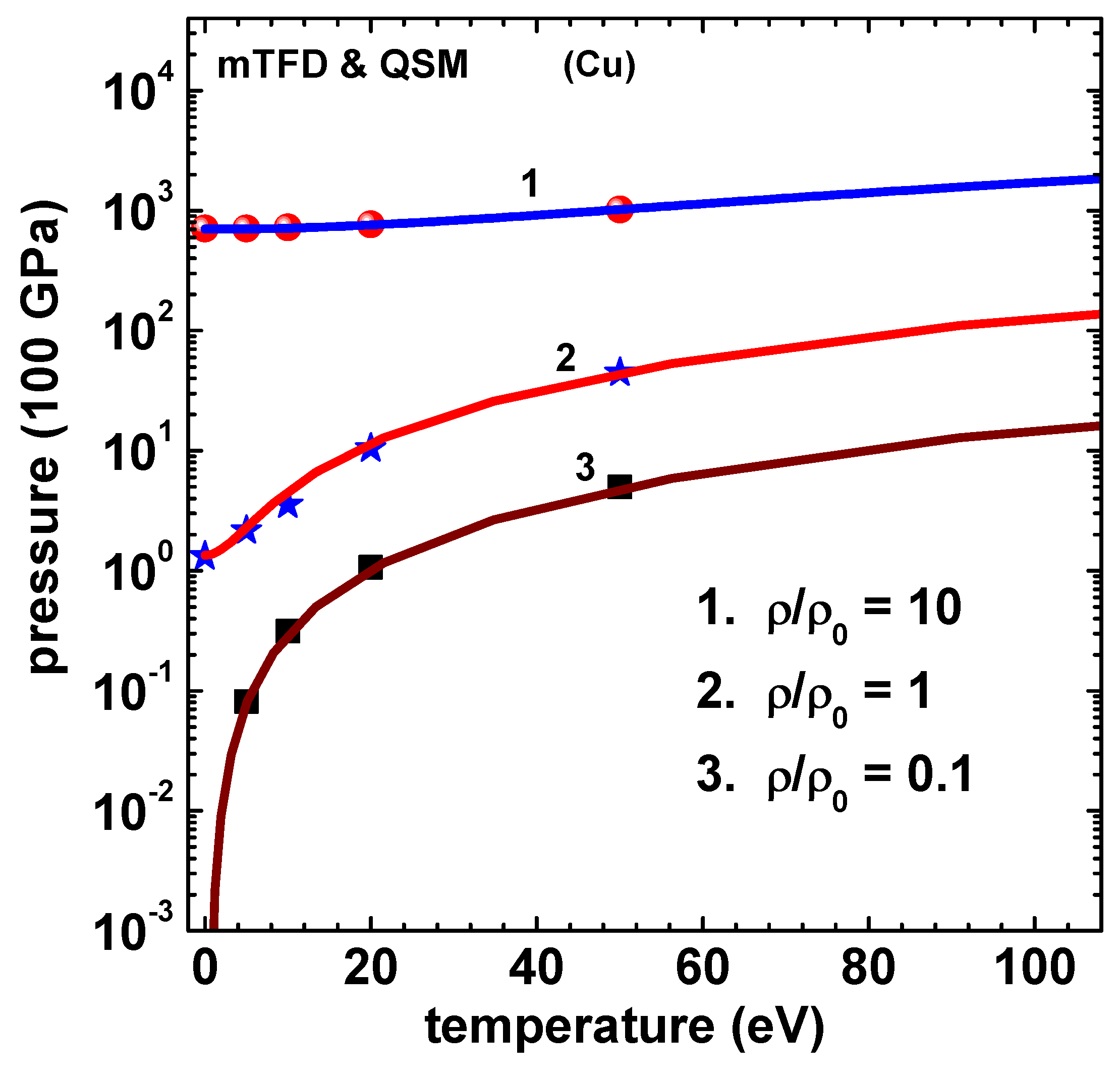
Figure 3.
Energy (100 kJ/g) versus temperature (eV) of Cu using mTFD model of this paper (lines) and finite-temperature-QSM (symbols) [10]. Curves marked 1, 2 and 3, respectively, correspond to , 1, and 0.1 , where . Data for Curve-2 and Curve-1 are shifted up by 30 and 60 units, respectively.
Figure 3.
Energy (100 kJ/g) versus temperature (eV) of Cu using mTFD model of this paper (lines) and finite-temperature-QSM (symbols) [10]. Curves marked 1, 2 and 3, respectively, correspond to , 1, and 0.1 , where . Data for Curve-2 and Curve-1 are shifted up by 30 and 60 units, respectively.
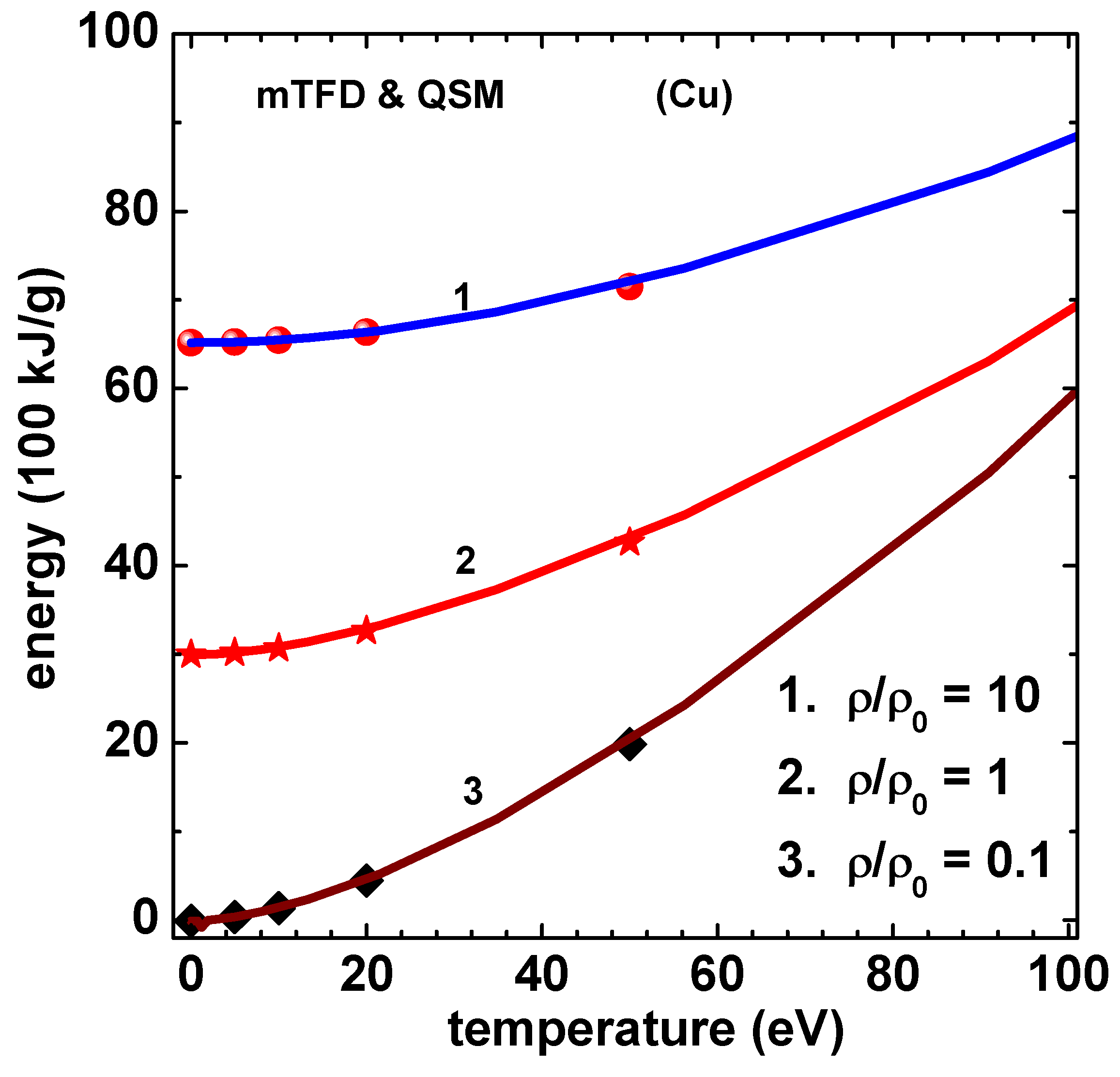
Figure 4.
Various components of energy (100 kJ/g) versus temperature (eV) of Cu using mTFD model of this paper. Density ratio is . The lines are for kinetic (curve-1), gradient (exchange part only) (curve-2), exchange-correlation (curve-3), and potential (curve-4). Data for kinetic and potential are divided by 20.
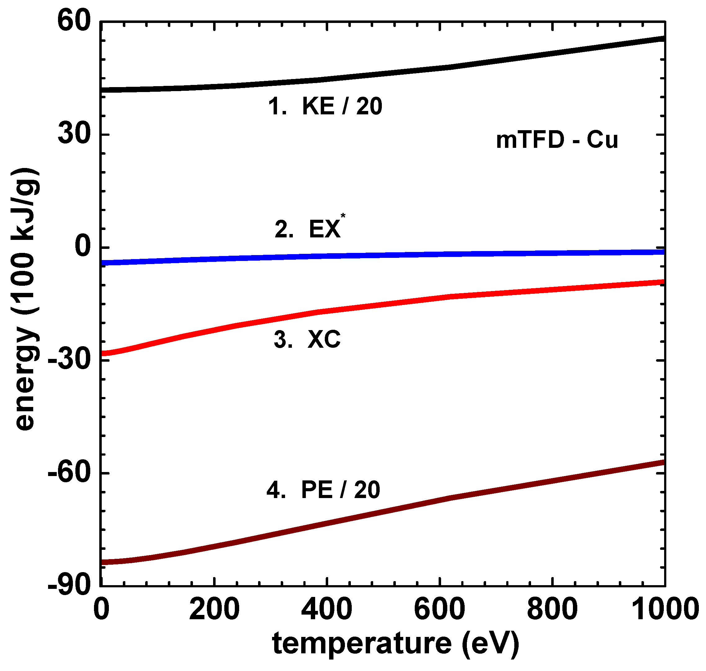
Figure 5.
Pressure (100 GPa) versus temperature (eV) of Al using mTFD model of this paper (lines) and finite-temperature-QSM (symbols) [10]. Curves marked 1, 2 and 3, respectively, correspond to , 1, and 0.1 , where .
Figure 5.
Pressure (100 GPa) versus temperature (eV) of Al using mTFD model of this paper (lines) and finite-temperature-QSM (symbols) [10]. Curves marked 1, 2 and 3, respectively, correspond to , 1, and 0.1 , where .
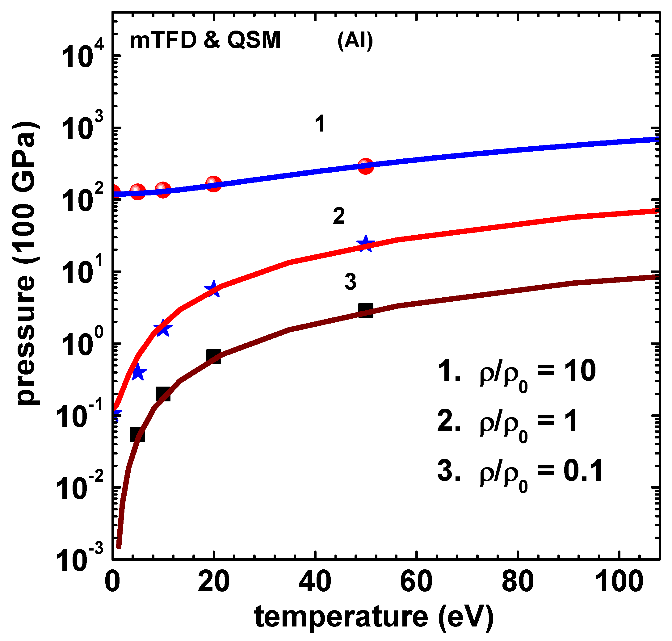
Figure 6.
Energy (100 kJ/g) versus temperature (eV) of Al using mTFD model of this paper (lines) and finite-temperature-QSM (symbols) [10]. Curves marked 1, 2 and 3, respectively, correspond to , 1, and 0.1 , where . Data for Curve-2 and Curve-1 are shifted up by 30 and 60 units, respectively.
Figure 6.
Energy (100 kJ/g) versus temperature (eV) of Al using mTFD model of this paper (lines) and finite-temperature-QSM (symbols) [10]. Curves marked 1, 2 and 3, respectively, correspond to , 1, and 0.1 , where . Data for Curve-2 and Curve-1 are shifted up by 30 and 60 units, respectively.
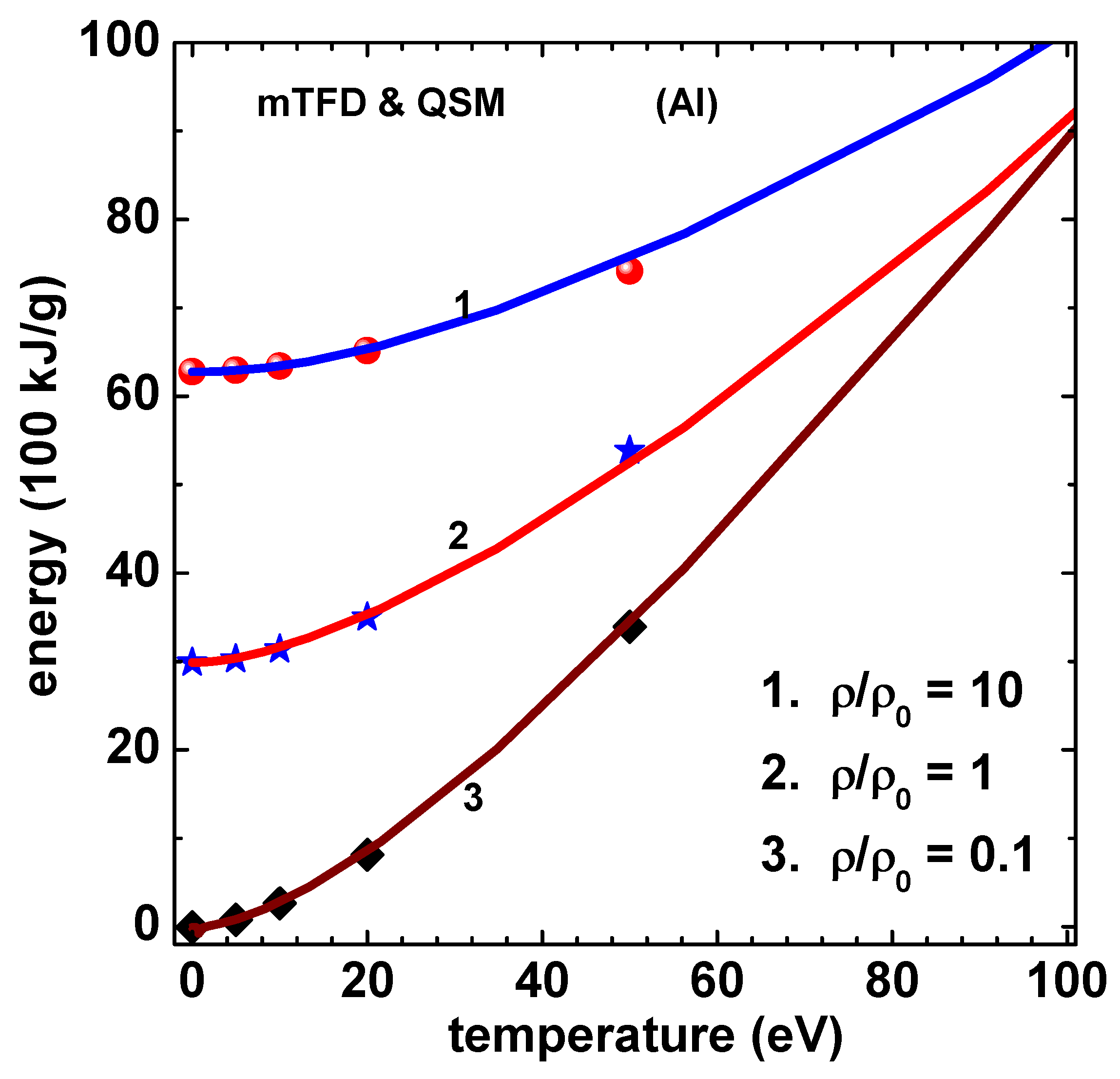
Figure 7.
Charge versus temperature (eV) of Al for different densities using mTFD model of this paper. Density ratio are 10 (curve-1), 2 (curve-2), 1 (curve-3) and 0.1 (curve-4). ( at 300 K are 5.06 and 0.966 for and 2, respectively). Values of using Eq.(22 (curve-1) and (curve-2), for , are compared in the inset figure.
Disclaimer/Publisher’s Note: The statements, opinions and data contained in all publications are solely those of the individual author(s) and contributor(s) and not of MDPI and/or the editor(s). MDPI and/or the editor(s) disclaim responsibility for any injury to people or property resulting from any ideas, methods, instructions or products referred to in the content. |
© 2025 by the author. Licensee MDPI, Basel, Switzerland. This article is an open access article distributed under the terms and conditions of the Creative Commons Attribution (CC BY) license (https://creativecommons.org/licenses/by/4.0/).
Copyright: This open access article is published under a Creative Commons CC BY 4.0 license, which permit the free download, distribution, and reuse, provided that the author and preprint are cited in any reuse.


