
Submitted:
16 December 2025
Posted:
17 December 2025
You are already at the latest version
Abstract
Accurate load identification serves as a fundamental requirement for achieving lightweight and efficient structural designs. This paper presents a dynamic load identification method for structures with parameter uncertainties, integrating the ellipsoidal model with shape functions. The approach explicitly accounts for correlations among uncertain structural parameters, leading to improved identification accuracy and more compact load bounds. The method first establishes an ellipsoidal model for the uncertain parameters, representing their feasible domain as a compact ellipsoidal set. This model is then incorporated into the dynamic load identification framework. Convex optimization theory and the Lagrangian multiplier method are employed to derive analytical expressions for the load bounds. Shape functions are utilized to describe the temporal variation of the load, reducing the ill-posedness of the inverse problem, while central finite difference approximations are applied to compute load sensitivities with respect to the uncertain parameters. The efficacy of the proposed method is validated through a numerical example involving a 21-bar truss structure, demonstrating its advantages in both identification accuracy and boundary compactness compared to conventional interval methods.
Keywords:
dynamic load identification
; uncertain structures
; correlation
; ellipsoid model
; interval model
1. Introduction
With the rapid advancement of contemporary industrial structures and manufacturing equipment toward larger scales, increased complexity, and technological sophistication, vibration and reliability concerns have gained prominence. Consequently, the scientific analysis of structural vibration states and the enhancement of structural reliability have emerged as important challenges. Dynamic loads, as fundamental excitation inputs, critically influence structural design optimization, vibration mitigation strategies, and reliability assessments [1,2,3]. However, in numerous practical scenarios, external dynamic loads prove challenging or unfeasible to measure directly due to adverse environmental conditions or prohibitive costs [4]. This limitation has motivated the development of indirect approaches that leverage measurable structural responses and system models for dynamic load identification.
Traditional dynamic load identification methodologies have been extensively developed under the assumption of deterministic structures with precisely known parameters [5], providing valuable frameworks and robust solutions for many engineering applications. However, in practical engineering scenarios, uncertainties arising from manufacturing tolerances, material variability, and measurement inaccuracies are inevitable [6]. These uncertainties may limit the direct applicability of deterministic methods and affect the reliability of identification results, particularly when parameter correlations are present. Therefore, extending load identification techniques to handle uncertain structures while accounting for parameter interdependencies becomes an important and complementary research direction.
Research on dynamic load identification for uncertain structures lies at the intersection of inverse problems and stochastic or non-probabilistic structural analysis. The need for dynamic load identification was recognized as early as the 1970s in fields such as military aviation, primarily to determine loads on propeller shafts [7]. Over time, two principal methodological categories have emerged: frequency-domain and time-domain approaches [8]. Frequency-domain techniques determine the dynamic load spectrum through the system's transfer function and response spectrum. Time-domain methods, developed subsequently, utilize the convolution relationship between load and response to reconstruct the load history. Beyond these, various innovative approaches have been proposed, including time-domain Galerkin methods [9], support vector regression techniques [10], neural network strategies [11], wavelet transform methodologies [12], and Kalman filter approaches [13]. It is noteworthy that these methodologies commonly assume structures to be deterministic.
In engineering practice, structural complexities, material inhomogeneity, and potential errors during manufacturing, installation, and measurement invariably introduce approximations and uncertainties into the structural models used for load identification. Parameters such as physical properties (mass, damping, stiffness), geometric characteristics, and boundary conditions [14] may all exhibit uncertainty. The influence of these uncertain parameters can lead to significant deviations from accurate results if deterministic load identification methods are applied without considering such uncertainties.
Research on uncertain structures originated with perturbation methods [15]. Monte Carlo simulation (MCS) [16] is a widely adopted technique for simulating random structures and often serves as a benchmark for assessing the accuracy of numerical methods. For solving differential equations with random coefficients, Moghaddam et al. [17] introduced an approximation approach based on expanding displacement using Hermite orthogonal polynomials, later recognized as the polynomial chaos expansion method. While probabilistic models can offer high theoretical accuracy [18,19,20], they require knowledge of the joint probability density function (PDF) of all uncertain parameters, and extensive sampling is often needed. In many practical engineering scenarios, acquiring sufficient data to characterize these PDFs accurately remains challenging. In some cases, even the underlying probability distributions themselves may be uncertain. In contrast, delineating the potential bounds of structural uncertainties is often more feasible [21,22,23,24,25]. Non-probabilistic models, operating under the premise of bounded uncertainties, require only the bounds of uncertain parameters. The output is then a set encompassing all feasible solutions, which can be more aligned with practical applications when data is scarce. Research into load identification for uncertain structures has seen various approaches: Lombardi [26] addressed uncertain optimization using anti-optimization strategies; Liu et al. [27,28] developed interval-based load identification methods; Wang et al. [29] introduced a fast iterative regularization approach; He et al. [30] advanced techniques to mitigate transducer damage; Yang [31] proposed an uncertainty-oriented regularization method; Wang et al. [32] approximated spatiotemporal dynamic loads via Chebyshev orthogonal polynomials; and Wu et al. [33] transformed uncertain system load identification into equivalent deterministic problems.
While the aforementioned studies have significantly advanced the field of load identification for uncertain structures, the explicit consideration of correlations among uncertain parameters remains an area that merits further investigation. Incorporating such correlations can potentially refine identification accuracy and lead to tighter uncertainty bounds, which is particularly beneficial for lightweight and efficient structural design.
Addressing this aspect, this study introduces an integrated methodology grounded in ellipsoidal modeling and shape functions. This approach provides a natural way to handle parameter correlations while maintaining implementation simplicity and achieving good identification precision. The remainder of this paper is organized as follows: Section 2 provides a comprehensive problem formulation. Section 3 elaborates the proposed methodology, detailing ellipsoidal modeling, problem transformation, and shape function implementation. Section 4 presents numerical validation through a 21-bar truss case study with thorough discussion. Section 5 concludes with key findings and future research directions.
2. Problem Formulation
Dynamic load identification aims to establish a mapping between measurable structural responses and unknown external loads, often stabilized through regularization techniques to mitigate ill-posedness. In deterministic settings, this mapping-often referred to as the solution model-yields unique load estimates based on precisely known structural parameters. However, real-world structures inevitably exhibit uncertainties in material properties, geometric dimensions, boundary conditions, and other parameters due to manufacturing variations, environmental effects, and measurement limitations. These uncertainties propagate into the solution model, transforming the load identification problem into a non-deterministic one. Consequently, reliable load estimation must not only address the ill-posed nature of the inverse problem but also account for the influence of parameter uncertainties and their potential correlations.
Considering uncertain parameters , the load identification model can be represented as:
(1)
where denotes the deterministic structural dynamic response with respect to time t, while F and f represent the solution model and dynamic load, respectively, both constituting function sets compatible with the uncertain parameters rather than unique deterministic functions. The existence of parameter uncertainty creates disparities between structural models and actual structures. Consequently, loads identified based on specific deterministic structural parameters represent only one possible scenario among many. When significant disparities exist between assumed and actual structural parameters, identified loads may deviate substantially from reality, potentially leading to misleading information or even structural failures.. Therefore, developing methods that systematically incorporate uncertainties for reliable load identification becomes imperative.
Traditional interval models represent uncertain parameters as , where superscripts I, L and U denote interval, lower bound, and upper bound, respectively. Under the assumption of small parameter variations, the uncertain load can be approximated through first-order Taylor expansion around parameter medians:
(2)
where and represent the median and perturbation of , respectively, while denotes the first-order derivative of the identified load at with respect to the uncertain parameter , and K indicates the number of uncertain parameters.
Based on the uncertain-but-bounded assumption, load identification for uncertain structures transforms into determining maximum and minimum load values. Conventional interval approaches yield explicit solutions for load boundaries at time t through natural interval extension of Equation (2):
(3a)
(3b)
where and are the minimum and maximum values of all possible dynamic loads at time t, respectively, and represents the value range of .
Equation (3) reveals that uncertain parameters are implicitly assumed to be independent, neglecting potential correlations. However, due to physical relationships between parameters, common sources of uncertainty, and other factors, parameter correlation is often present in practical engineering problems. Accounting for these correlations and establishing a more compact feasible domain can contribute to obtaining tighter load bounds and higher-precision identification results, which holds significant practical importance.
3. Methodology
3.1. Ellipsoid Modeling of Structural Uncertain Parameters
To effectively capture and utilize correlations among structural parameters, this paper employs the non-probabilistic ellipsoid model. This approach describes the joint uncertainty domain of multiple interval parameters as a multidimensional ellipsoid, reflecting parameter uncertainty levels and correlations through the size and shape of the ellipsoid [34]. In the ellipsoid set, each element represents a possible realization of the uncertain parameters. For two correlated interval parameters and , the uncertainty domain can be described by an elliptic domain denoted as , as illustrated in Figure 1.
The covariance of the two interval parameters and is defined as
(4)
where and respectively represent the lengths of the two semi-axes of the ellipse. The correlation coefficient of interval parameters and is defined as:
(5)
which reveals the correlation characteristics between and . When , the parameters are positively correlated; when , they are negatively correlated; when , they are uncorrelated. A more compact elliptical uncertainty domain corresponds to a larger absolute value of calculated by Equation (5), indicating stronger correlation between parameters. If parameters are fully correlated (), the ellipse degenerates into a line.
For two interval parameters, the ellipse uncertainty domain can be expressed as:
(6)
For multiple correlated interval parameters, the high-dimensional ellipsoidal uncertainty domain can be expressed as:,
(7)
where W is the symmetric positive definite characteristic matrix of the ellipsoid, reflecting the size and shape of the uncertainty domain. Equation (7) shows that constructing an n-dimensional ellipsoid domain essentially equates to determining W. In practical computation, the correlation analysis technique [35] is adopted, establishing the relationship between W and the covariance matrix of uncertain parameters as follows:
(8)
3.2. Load Identification Based on Ellipsoid Model
Assuming structural parameter uncertainties exhibit small variations, the dynamic load can be approximated through first-order Taylor expansion around uncertain parameter medians. Utilizing the constructed ellipsoid model, which incorporates correlation characteristics, the determination of dynamic load lower and upper bounds transforms into the following optimization problems:
(9a)
(9b)
In these optimization problems, the objective function is linear and the feasible domain constitutes a convex set. According to convex optimization theory [36], optimal points for Equations (9a) and (9b) must reside on the feasible domain boundary. Consequently, the Lagrange multiplier method is introduced to solve these problems. The Lagrange function L is constructed as:
(10)
where denotes the Lagrange multiplier, and is introduced for notational convenience.
To determine extreme points of Equation (10), the gradient of function L with respect to uncertain parameters is computed:
(11)
The extreme points are obtained by setting Equation (11) equal to zero:
(12)
Substituting Eq. (12) into the ellipsoid equation yields:
(13)
Substituting Equations (13) and (12) into Equation (2), the lower and upper load bounds are obtained as:
(14a)
(14b)
Comparing Equation (14) with Equation (3), the solutions utilizing the ellipsoid model incorporate parameter correlation, which can contribute to more accurate and compact results. However, realizing load identification for uncertain structures still requires the identification of load medians and computation of load gradients .
3.3. Identification of Load Median by Using Shape Functions
To reconstruct , median values of uncertain parameters are substituted into the structural model. According to the Green's kernel function method (GKFM) [1], the forward problem of dynamic load identification at these median values assumes the following convolution integral form:
(15)
where refers to the Green's kernel function. By approximating the load through a series of square wave functions, GKFM assumes the load remains constant within each discrete sampling time interval. However, since the actual load variation within time intervals is unknown, accurately describing the load typically requires sufficiently small time intervals. This, in turn, increases the scale of the Green's kernel function matrix, exacerbating computational burden and ill-conditioning.
To address this issue, shape functions are adopted in this paper, enabling load description through specific functional forms within time intervals and reducing ill-posedness. The load is initially divided into m elements in the time domain, with n time nodes assumed within each time element. In the i-th element, the modal load can be locally approximated by linear combination of n linearly independent basis functions:
(16)
where approximates the load median in the i-th time element, while and respectively represent linearly the independent basis functions and coefficients. Taking the n nodes in the time element as interpolation control points, the coefficient vector is solved as:
(17)
where , , and represents the basis function matrix with elements . Substituting Equation (17) into Equation (16) yields:
(18)
Denoting , represents the shape functions of the load in the time element. Since identical basis functions are used in each time element, load shape functions remain consistent across elements. Therefore, across the entire time domain, the load can be obtained by assembling approximate dynamic loads from all time elements:
(19)
Notably, and of two adjacent time elements represent the same load sampling point. Based on the linear system superposition principle, the response can be expressed as:
(20)
Denoting:
(21)
(22)
(23)
It can be obtained that
(24)
And in discrete form:
(25)
When multiple dynamic loads act on the structure, according to the superposition principle of linear time-varying structures, structural responses can be correspondingly expressed as:
(26)
where and represent the i-th load and j-th structural response, respectively, denotes the Green's kernel matrix from the i-th loading point to the j-th measuring point, and P indicates the number of loads. For notational convenience, Equation (26) is still abbreviated as without loss of generality.
When solving the load based on Equation (25), matrix H is often ill-conditioned. Direct matrix inversion would seriously amplify errors in measured responses, causing obtained load medians to substantially deviate from true values. To improve solution stability, the Tikhonov regularization method [37] is employed to suppress noise influence, yielding the following stable approximate solution:
(27)
where and denote the computed load and measured response, respectively. Matrix is singular value decomposed [38] as , where , , and represent its singular matrices and non-negative singular values, while denotes the Tikhonov regularization filter function. The optimal regularization parameter is determined by the L-curve method [39].
After acquiring the load median , gradients with respect to each uncertain parameter are computed using central finite difference approximations:
(28)
where stands for the variation vector of uncertain parameters, sharing the same dimension as . When , only the k-th parameter is perturbed by a small bias . The corresponding load is identified using the shape function method with regularization, and the load gradient with respect to the parameter is calculated according to Equation (28). Ultimately, the lower and upper boundaries from Equation (14) can be obtained.
4. Numerical Example and Discussion
4.1. Example Setup
To verify the proposed method's effectiveness and demonstrate its detailed implementation, the load identification problem for a 21-bar truss structure, illustrated in Figure 2, is considered. Transverse and longitudinal bars have lengths of 5m, material Poisson's ratio is 0.3, and proportional damping is assumed with a stiffness matrix correlation coefficient of 3×10⁻³. Nodes 1, 2, 3, and 4 are hinge-supported. Two dynamic loads, as shown in Figure 2, act on Node 7 and Node 10 along horizontal and vertical directions, respectively, with forms of N and N, where . Elastic modulus E, cross-sectional area A, and density d of the truss are assumed uncertain. The uncertainty level (ucl) of parameters is 10%, with median values , and . These three uncertain parameters exhibit certain correlations: , , . To simulate real measurement environments, noise is introduced into calculated responses as follows:
(29)
where denotes the noise polluted response, computes the standard deviation of response , is the noise level, and generates random numbers falling in [[-1,1].
Initially, following the correlation modeling technique described in Section 3.1, the approximate ellipsoid model for these uncertain parameters is established as Equation (30) and illustrated in Figure 3. Evidently, the established ellipsoidal model is more compact compared to the volumetric interval model, offering a more precise representation of uncertain parameter distribution. Employing this ellipsoidal model for load identification is anticipated to yield more accurate results.
(30)
As the measured responses have a direct impact on the accuracy of identification results, the measuring points are to be selected. On the one hand, the measuring points should be close to the loading points so that the responses can be ensured with high signal-to-noise ratio; on the other hand, the measuring responses should be as uncorrelated as possible so as to improve the stability when solving the inverse problem. In view of this, the horizontal direction of Node 5 and vertical direction of Node 8 are selected for response measurement. To simulate real conditions, structural measuring responses are randomly calculated under , and , with 10% noise level added per Equation (29). The two measured responses are shown in Figure 4. Both responses exhibit significant magnitudes, and distinctive response patterns can be intuitively observed, confirming their suitability for load identification.
4.2. Load Identification Results
According to the proposed method, load identification decomposes into load median identification and load boundary determination. For the first subproblem, median values of structural uncertain parameters,, and , are substituted into the structural numerical model. As mentioned in Section 3.3, GKFM approximates loads as constants within sampling time intervals, creating a dilemma where accuracy and ill-posedness cannot be simultaneously balanced. To improve this situation, shape functions are employed, enabling kernel matrix scale control while enhancing description accuracy.
In this example, the load is divided into 199 time elements within the 0.4s time domain. Each time element contains 2 time nodes, with a time interval of 0.002s. The employed shape functions take the forms and , where . Applying linear shape function loads described by and at actual truss loading points, combined responses of corresponding linear shape function loads are determined through two separate finite element analyses. In the discrete time domain, analogous to finite element stiffness matrix assembly, responses of linear shape function loads for each discrete time element are aggregated, forming the kernel function response matrix across the entire time domain per Equation (23). Based on the established forward model of Equation (24), Tikhonov regularization is introduced to overcome inherent ill-posedness, acquiring stable and accurate results shown in Figure 5. Although certain deviations exist between identified and actual loads, they demonstrate high consistency. Typically, disparities between identified and true loads stem from two primary sources: inherent parameter discrepancies and inevitable identification process errors. While regularization ameliorates problem ill-posedness, it doesn't eradicate it entirely. Consequently, the solution represents an approximation endeavoring to approach the true value as closely as feasible.
Subsequently, gradients of dynamically identified loads at parameter medians with respect to each uncertain parameter are computed using central finite difference approximations. At each time instance, only one parameter is varied around its median value. The corresponding load is identified via the shape function method with regularization. Load gradients with respect to parameters are then calculated according to Equation (28). In this example, gradient curves of the two dynamic loads with respect to the three uncertain parameters are shown in Figure 6. The figure reveals that both dynamic loads exhibit sensitivity to uncertain parameters.
Finally, lower and upper load boundaries are calculated based on Equation (14) and depicted in Figure 7. For comparison, load intervals identified based on the traditional interval model are presented in Figure 8. Comparing Figure 7 and Figure 8 reveals that: (1) load boundaries identified using both ellipsoid and interval models effectively envelope real loads; (2) load boundaries established via the ellipsoid model exhibit more concise profiles compared to those derived from the interval model. This implies that considering parameter correlations proves highly beneficial for obtaining more accurate load identification results, playing a significant role in reducing structural design safety factors and promoting lightweight, efficient structural design.
4.3. Parameter Sensitivity and Robustness Analysis
To further investigate the influence of structural uncertain parameters on load identification, noise levels are adjusted to 5% and 15% while maintaining parameter uncertainty levels unchanged. Implementing the proposed method, identified load bounds are shown in Figure 9 and Figure 10. Under different noise levels, identified load boundaries exhibit considerable deviation, but interval sizes remain essentially unchanged. This indicates that measurement noise primarily affects load boundary forms rather than boundary ranges.
Further, under the noise level of 10%, the uncertainty level of the parameter is adjusted to 5% and 15%. The identified load bounds are shown in Figure 11 and Figure 12. It can be observed that the load range changes significantly under different uncertainty levels. As uncertainty levels increase, load bounds widen, with change amplitudes more substantial than those induced by noise increases.
4.4. Comparative Analysis with Monte Carlo Simulation
To further validate the proposed method's accuracy, a comparative analysis with Monte Carlo simulation (MCS) involving 10,000 samples was conducted under 10% parameter uncertainty level and 10% noise level. Table 1 presents boundary errors and computational times for both methods, demonstrating that the proposed approach achieves comparable accuracy to MCS with significantly reduced computational effort.
5. Conclusions
This study proposes an approach integrating a non-probabilistic ellipsoidal model with shape functions for identifying external dynamic loads in structures subject to parameter uncertainties. The ellipsoidal model provides an effective means to represent and utilize correlations among uncertain parameters, which are often overlooked in conventional interval methods. Based on the developed ellipsoidal model and Lagrangian formulation, explicit expressions for the bounds of structural dynamic loads are derived. The adoption of shape functions for load representation helps reduce the scale of the inverse problem and enhances numerical stability. The practical applicability and advantages of the proposed method are validated through a case study on a 21-bar truss structure.
The main features and advantages of the proposed method include:
(1) Effective incorporation of parameter correlations through ellipsoidal modeling, resulting in more compact and accurate identification bounds compared to independent interval analysis.
(2) Enhanced computational efficiency compared to sampling-based probabilistic approaches like Monte Carlo simulation.
(3) Improved numerical stability through the combined use of shape function representation and Tikhonov regularization.
(4) Demonstrated robustness under various levels of measurement noise and parameter uncertainty.
However, certain limitations should be noted. The method primarily applies to structures with relatively small uncertainty levels, as the first-order Taylor expansion may become less accurate under high uncertainty conditions. Future research directions include extending the methodology to handle larger uncertainties through higher-order expansions or other approximation schemes, developing adaptive or higher-order shape functions for improved load representation, and investigating applications to more complex structural systems with nonlinear dynamic behaviors.
Author Contributions
K.L., Conceptualization, Methodology, Investigation, Funding acquisition, Writing-review and editing; Z.F., Methodology, Investigation, Writing-review and editing; X.M., Investigation, Software, Data curation. N.C. and Y.C., Data curation, Writing-original draft. All authors have read and agreed to the published version of the manuscript.
Institutional Review Board Statement
Not applicable.
Informed Consent Statement
Not applicable.
Data Availability Statement
Detailed data are contained within the article.
Conflicts of Interest
The authors declare no conflict of interest.
References
- Liu, J.; Li, K. Sparse identification of time-space coupled distributed dynamic load. Mech. Syst. Signal Process. 2021, 148, 107177. [Google Scholar] [CrossRef]
- Yu, B.; Wu, Y.; Hu, P.; et al. A non-iterative identification method of dynamic loads for different structures. J. Sound Vib. 2020, 483, 115508. [Google Scholar] [CrossRef]
- Li, K.; Zhao, Y.; Fu, Z.; et al. Equivalent Identification of Distributed Random Dynamic Load by Using K-L Decomposition and Sparse Representation. Machines 2022, 10, 311. [Google Scholar] [CrossRef]
- Jia, Y.; Yang, Z.; Song, Q. Experimental study of random dynamic loads identification based on weighted regularization method. J. Sound Vib. 2015, 342, 113–123. [Google Scholar] [CrossRef]
- Xu, M.; Jiang, N. Dynamic load identification for interval structures under a presupposition of 'being included prior to being measured'. Appl. Math. Model. 2020, 85, 107–123. [Google Scholar] [CrossRef]
- Li, L.; Chen, G.; Fang, M.; et al. Reliability analysis of structures with multimodal distributions based on direct probability integral method. Reliab. Eng. Syst. Saf. 2021, 215, 107885. [Google Scholar] [CrossRef]
- Sanchez, J.; Benaroya, H. Review of force reconstruction techniques. J. Sound Vib. 2014, 333, 2999–3018. [Google Scholar] [CrossRef]
- Liu, R.; Dobriban, E.; Hou, Z.; et al. Dynamic load identification for mechanical systems: A review. Arch. Comput. Methods Eng. 2021, 28, 1–33. [Google Scholar] [CrossRef]
- Liu, J.; Meng, X.; Jiang, C.; et al. Time-domain Galerkin method for dynamic load identification. Int. J. Numer. Methods Eng. 2016, 105, 620–640. [Google Scholar] [CrossRef]
- Liu, Y.; Wang, L.; Gu, K. A support vector regression (SVR)-based method for dynamic load identification using heterogeneous responses under interval uncertainties. Appl. Soft Comput. 2021, 110, 107599. [Google Scholar] [CrossRef]
- Li, J.; Yan, J.; Zhu, J.; et al. K-BP neural network-based strain field inversion and load identification for CFRP. Measurement 2022, 187, 110227. [Google Scholar] [CrossRef]
- Ovanesova, A.V.; Suarez, L.E. Applications of wavelet transforms to damage detection in frame structures. Eng. Struct. 2004, 26, 39–49. [Google Scholar] [CrossRef]
- Li, H.; Jiang, J.; Mohamed, M.S. Online dynamic load identification based on extended Kalman filter for structures with varying parameters. Symmetry 2021, 13, 1372. [Google Scholar] [CrossRef]
- Wang, L.; Wang, X.; Xia, Y. Hybrid reliability analysis of structures with multi-source uncertainties. Acta Mech. 2014, 225, 413–430. [Google Scholar] [CrossRef]
- He, J.H. Homotopy perturbation method: a new nonlinear analytical technique. Appl. Math. Comput. 2003, 135, 73–79. [Google Scholar] [CrossRef]
- Lewis, E.E.; Böhm, F. Monte Carlo simulation of Markov unreliability models. Nucl. Eng. Des. 1984, 77, 49–62. [Google Scholar] [CrossRef]
- Moghaddam, V.H.; Hamidzadeh, J. New Hermite orthogonal polynomial kernel and combined kernels in support vector machine classifier. Pattern Recognit. 2016, 60, 921–935. [Google Scholar] [CrossRef]
- Mao, J.; Xiao, Y.; Yu, Z.; et al. Probabilistic model and analysis of coupled train-ballasted track-subgrade system with uncertain structural parameters. J. Cent. South Univ. 2021, 28, 2238–2256. [Google Scholar] [CrossRef]
- Liu, J.; Sun, X.; Han, X.; et al. Dynamic load identification for stochastic structures based on Gegenbauer polynomial approximation and regularization method. Mech. Syst. Signal Process. 2015, 56, 35–54. [Google Scholar] [CrossRef]
- Liu, J.; Sun, X.S.; Li, K.; et al. A probability density function discretization and approximation method for the dynamic load identification of stochastic structures. J. Sound Vib. 2015, 357, 74–94. [Google Scholar] [CrossRef]
- Rao, S.S.; Berke, L. Analysis of uncertain structural systems using interval analysis. AIAA J. 1997, 35, 727–735. [Google Scholar] [CrossRef]
- Qiu, Z.; Ma, Y.; Wang, X. Comparison between non-probabilistic interval analysis method and probabilistic approach in static response problem of structures with uncertain-but-bounded parameters. Commun. Numer. Methods Eng. 2004, 20, 279–290. [Google Scholar] [CrossRef]
- Jiang, C.; Lu, G.Y.; Han, X.; et al. A new reliability analysis method for uncertain structures with random and interval variables. Int. J. Mech. Mater. Des. 2012, 8, 169–182. [Google Scholar] [CrossRef]
- Xia, B.; Wang, L. Non-probabilistic interval process analysis of time-varying uncertain structures. Eng. Struct. 2018, 175, 101–112. [Google Scholar] [CrossRef]
- Ni, B.Y.; Jiang, C.; Han, X. An improved multidimensional parallelepiped non-probabilistic model for structural uncertainty analysis. Appl. Math. Model. 2016, 40, 4727–4745. [Google Scholar] [CrossRef]
- Lombardi, M. Optimization of uncertain structures using non-probabilistic models. Comput. Struct. 1998, 67, 99–103. [Google Scholar] [CrossRef]
- Liu, J.; Han, X.; Jiang, C.; et al. Dynamic load identification for uncertain structures based on interval analysis and regularization method. Int. J. Comput. Methods 2011, 8, 667–683. [Google Scholar] [CrossRef]
- Liu, J.; Sun, X.; Meng, X.; et al. A novel shape function approach of dynamic load identification for the structures with interval uncertainty. Int. J. Mech. Mater. Des. 2016, 12, 375–386. [Google Scholar] [CrossRef]
- Wang, L.; Peng, Y.; Xie, Y.; et al. A new iteration regularization method for dynamic load identification of stochastic structures. Mech. Syst. Signal Process. 2021, 156, 107586. [Google Scholar] [CrossRef]
- He, Z.C.; Zhang, Z.; Li, E. Random dynamic load identification for stochastic structural-acoustic system using an adaptive regularization parameter and evidence theory. J. Sound Vib. 2020, 471, 115188. [Google Scholar] [CrossRef]
- Yang, C. A novel uncertainty-oriented regularization method for load identification. Mech. Syst. Signal Process. 2021, 158, 107774. [Google Scholar] [CrossRef]
- Wang, L.; Liu, Y.; Liu, Y. An inverse method for distributed dynamic load identification of structures with interval uncertainties. Adv. Eng. Softw. 2019, 131, 77–89. [Google Scholar] [CrossRef]
- Wu, S.; Sun, Y.; Li, Y.; et al. Stochastic dynamic load identification on an uncertain structure with correlated system parameters. J. Vib. Acoust. 2019, 141, 041009. [Google Scholar] [CrossRef]
- Jiang, C.; Han, X.; Lu, G.Y.; et al. Correlation analysis of non-probabilistic convex model and corresponding structural reliability technique. Comput. Methods Appl. Mech. Eng. 2011, 200, 2528–2546. [Google Scholar] [CrossRef]
- Jiang, C.; Bi, R.G.; Lu, G.Y.; et al. Structural reliability analysis using non-probabilistic convex model. Comput. Methods Appl. Mech. Eng. 2013, 254, 83–98. [Google Scholar] [CrossRef]
- Bertsekas, D. Convex Optimization Theory; Athena Scientific: Belmont, MA, USA, 2009. [Google Scholar]
- Golub, G.H.; Hansen, P.C.; O'Leary, D.P. Tikhonov regularization and total least squares. SIAM J. Matrix Anal. Appl. 1999, 21, 185–194. [Google Scholar] [CrossRef]
- Abdi, H. Singular value decomposition (SVD) and generalized singular value decomposition. In Encyclopedia of Measurement and Statistics; Salkind, N.J., Ed.; Sage: Thousand Oaks, CA, USA, 2007; pp. 907–912. [Google Scholar]
- Calvetti, D.; Morigi, S.; Reichel, L.; et al. Tikhonov regularization and the L-curve for large discrete ill-posed problems. J. Comput. Appl. Math. 2000, 123, 423–446. [Google Scholar] [CrossRef]
Figure 1.
Schematic of the ellipsoidal (elliptic) correlation model for two uncertain parameters.
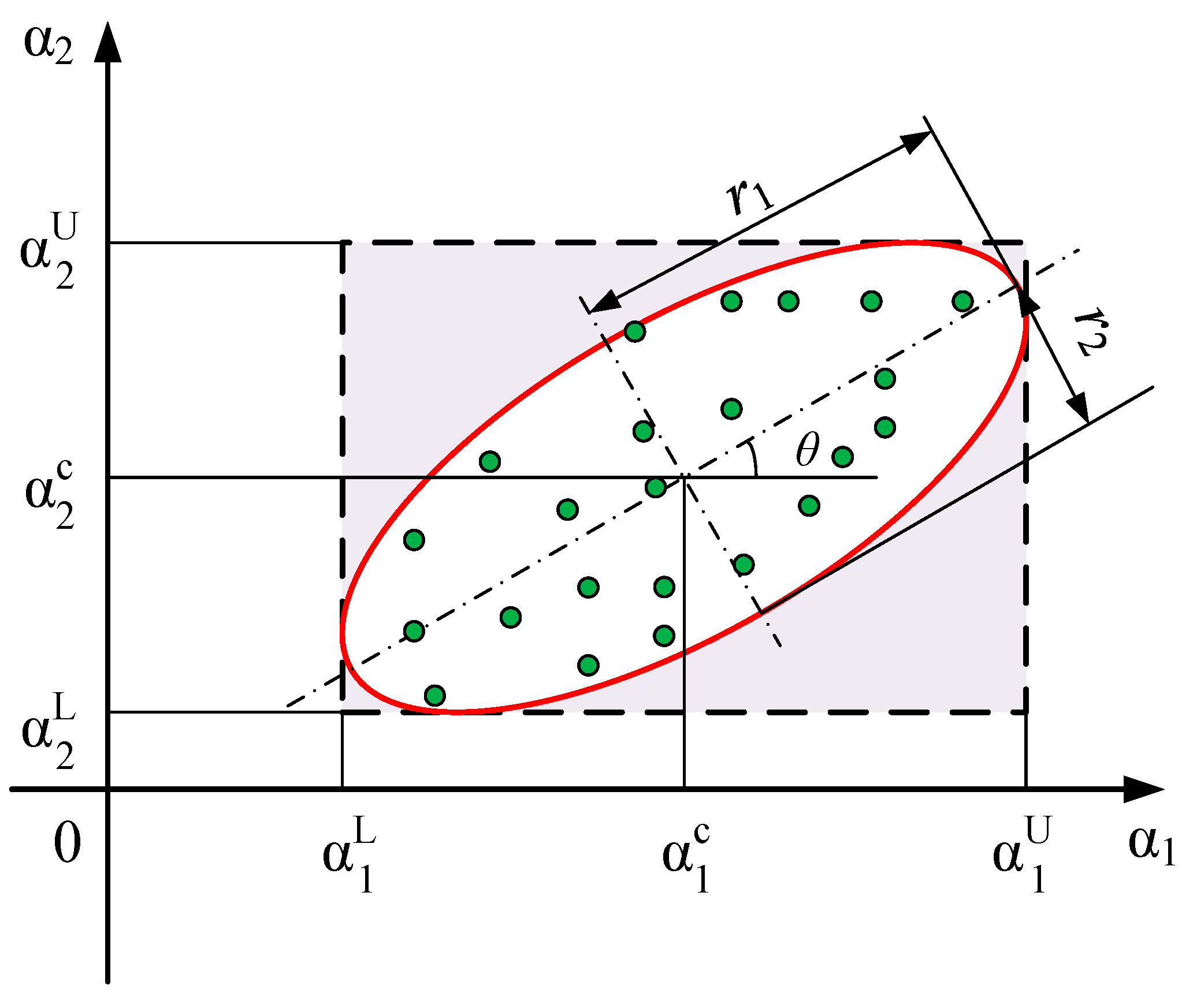
Figure 2.
The 21-bar truss structure.
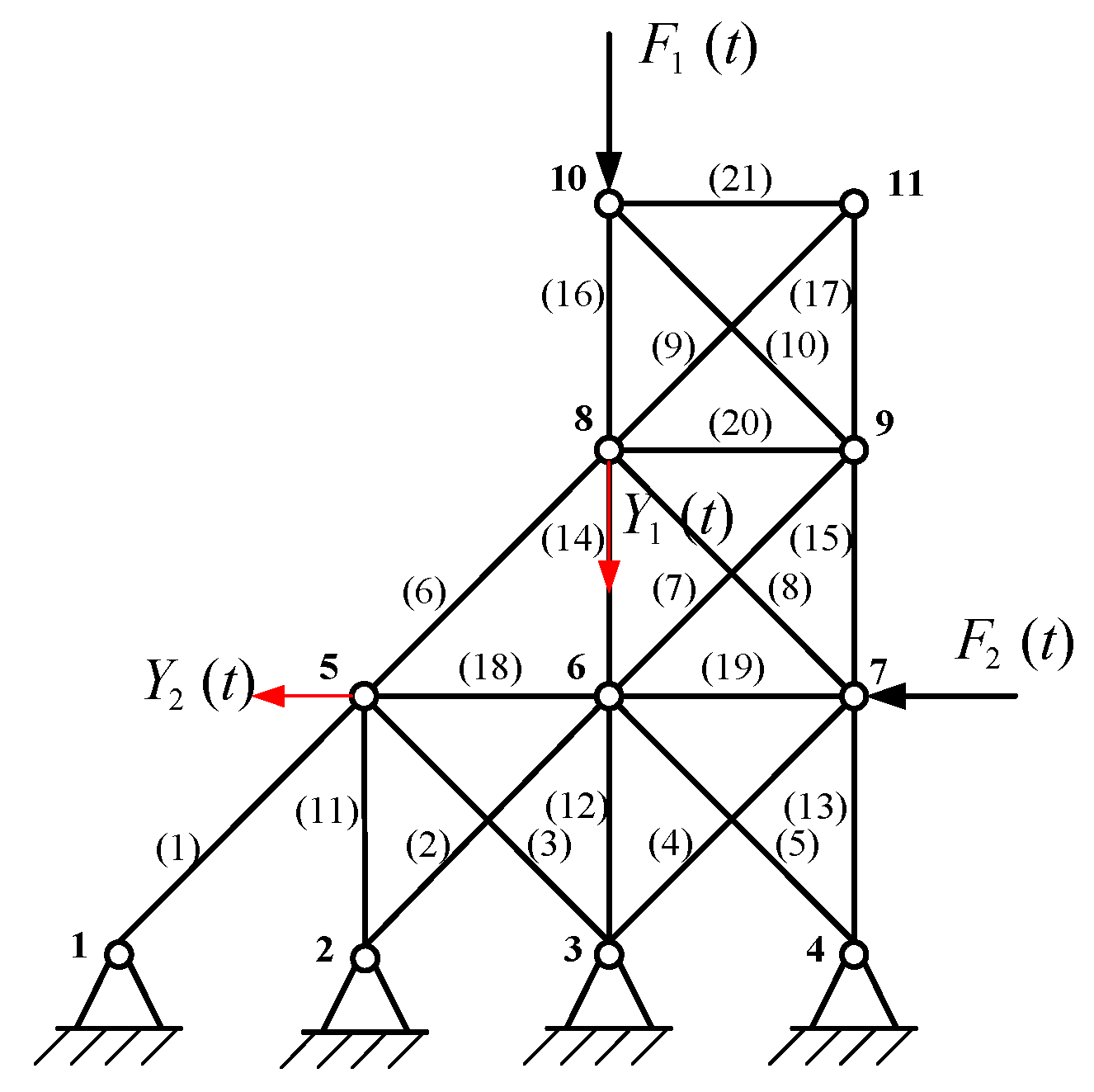
Figure 3.
The ellipsoid model of the uncertain parameters E, A, and ρ.
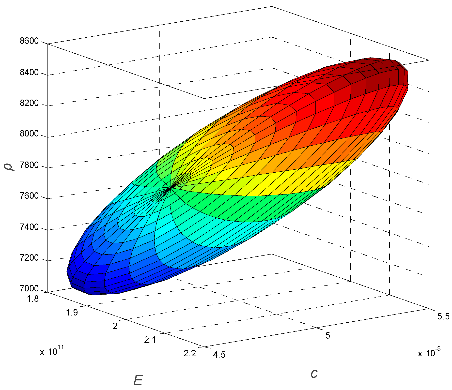
Figure 4.
Measured displacement responses used for load identification: (a) horizontal displacement at Node 5; (b) vertical displacement at Node 8.
Figure 4.
Measured displacement responses used for load identification: (a) horizontal displacement at Node 5; (b) vertical displacement at Node 8.
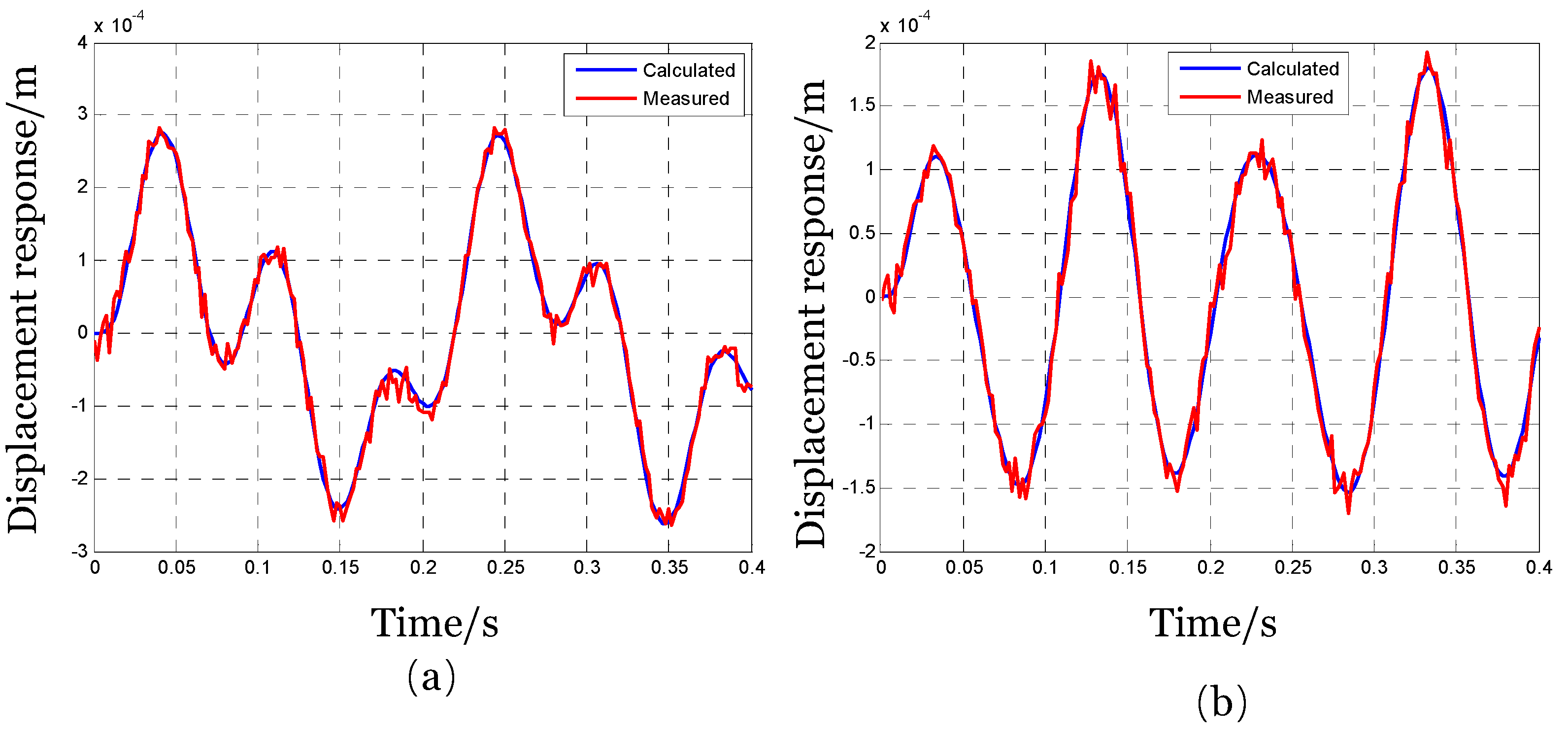
Figure 5.
Dynamic loads identified at median values of uncertain parameters ((a): Load f1; (b): Load f2).
Figure 5.
Dynamic loads identified at median values of uncertain parameters ((a): Load f1; (b): Load f2).
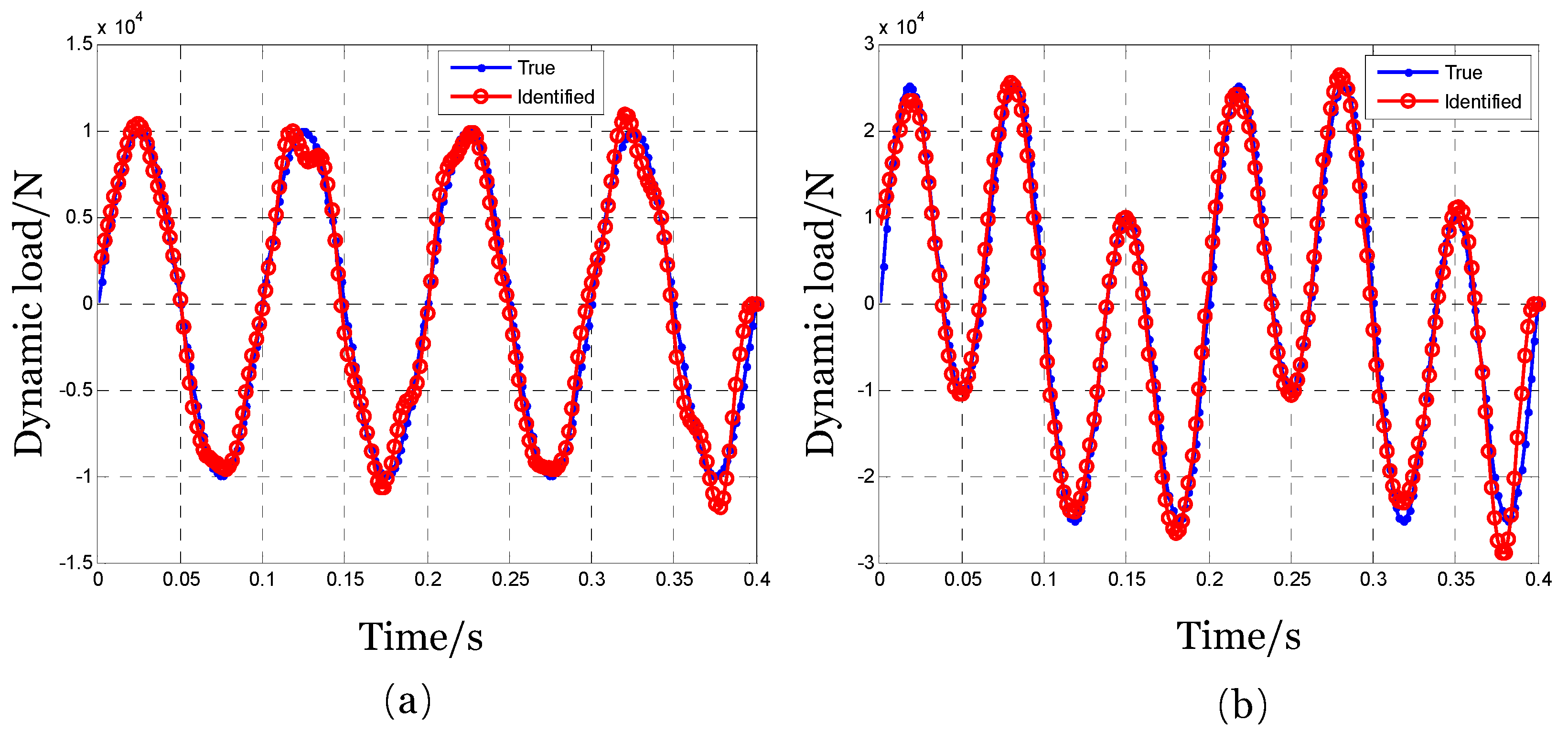
Figure 6.
Gradients of the loads with respect to the uncertain parameters (Blue line: ; Red line: ).
Figure 6.
Gradients of the loads with respect to the uncertain parameters (Blue line: ; Red line: ).
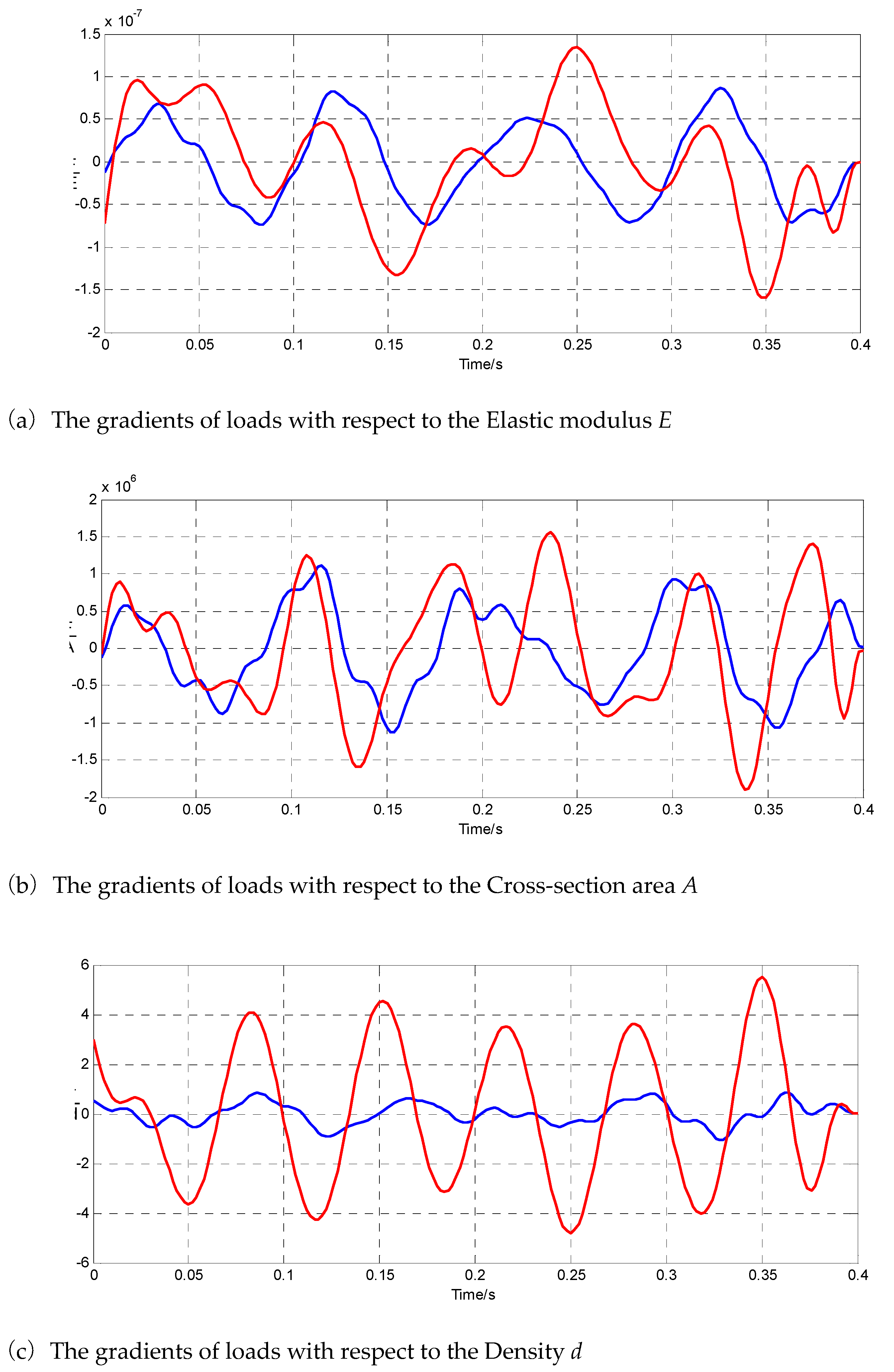
Figure 7.
Load bounds identified using the proposed ellipsoid model under , .
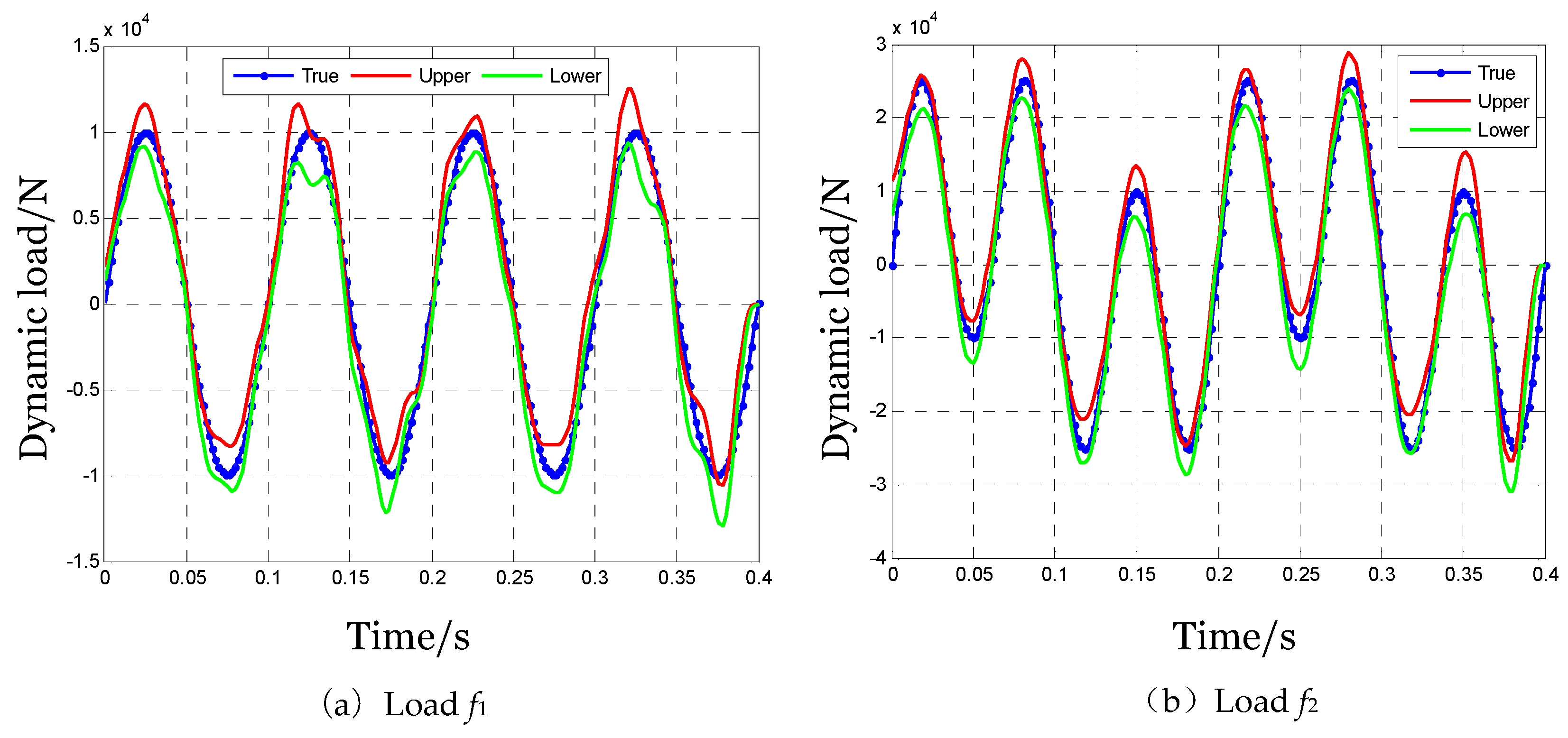
Figure 8.
Load bounds identified using the conventional interval model under , .
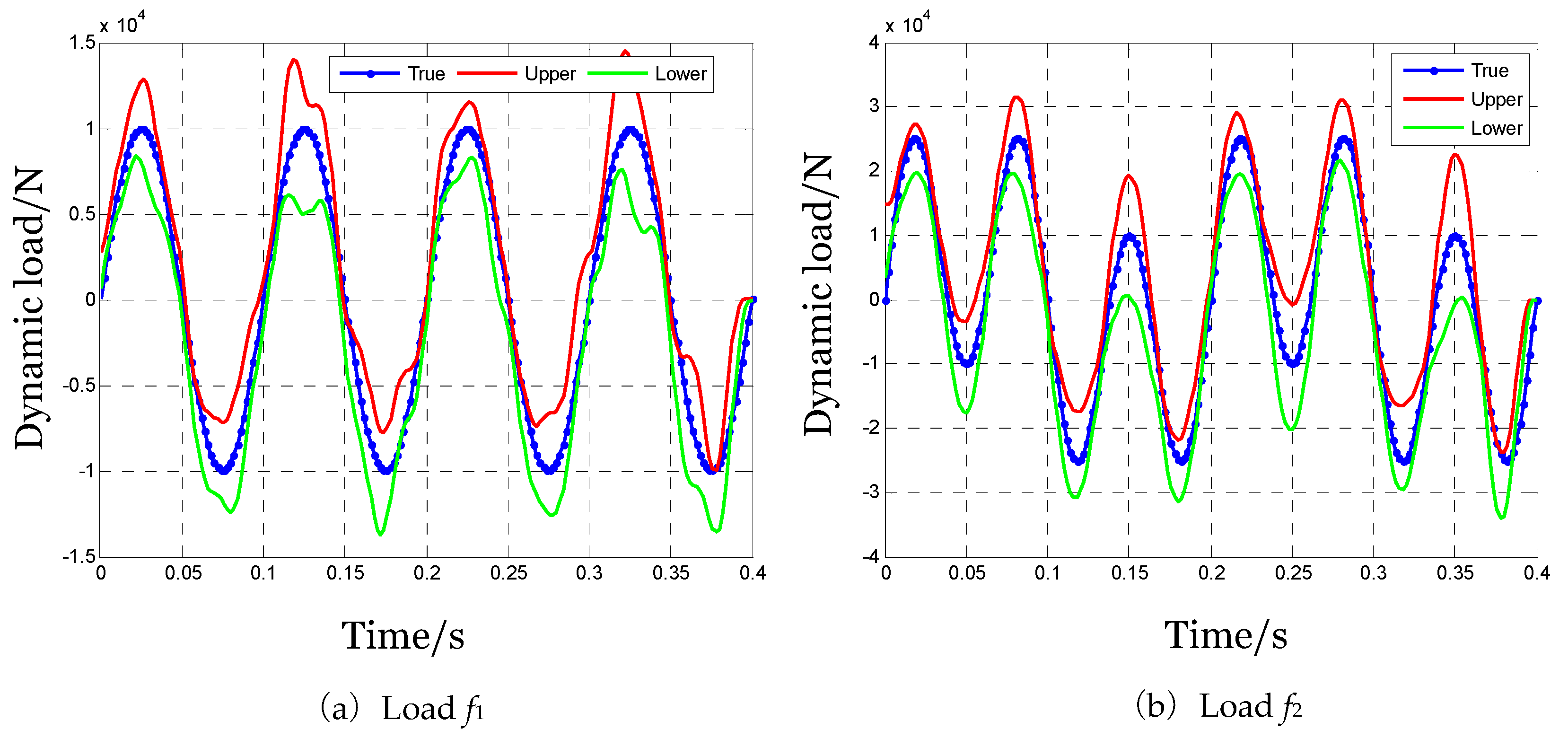
Figure 9.
Load bounds identified using the ellipsoid model under , .
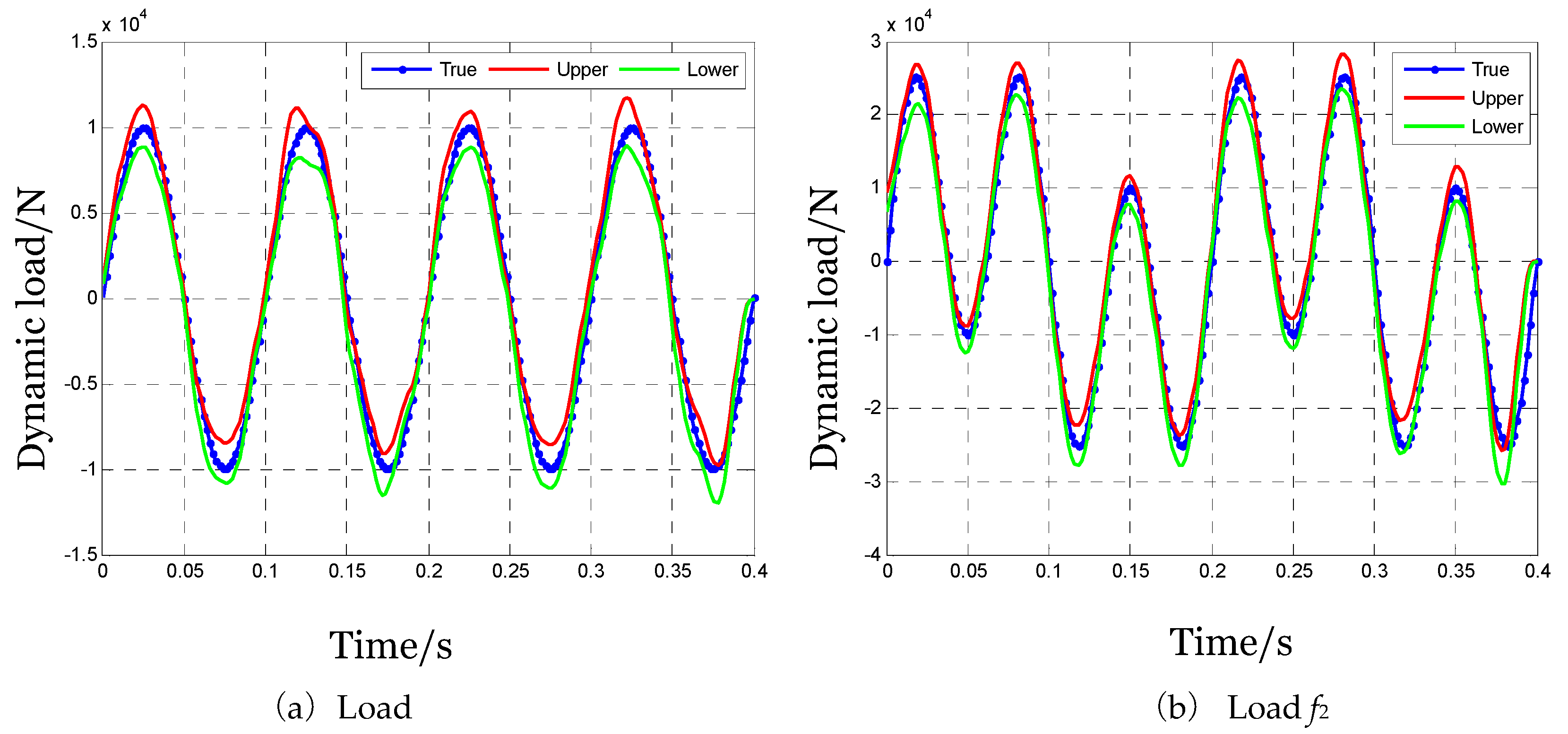
Figure 10.
Load bounds identified using the ellipsoid model under , .
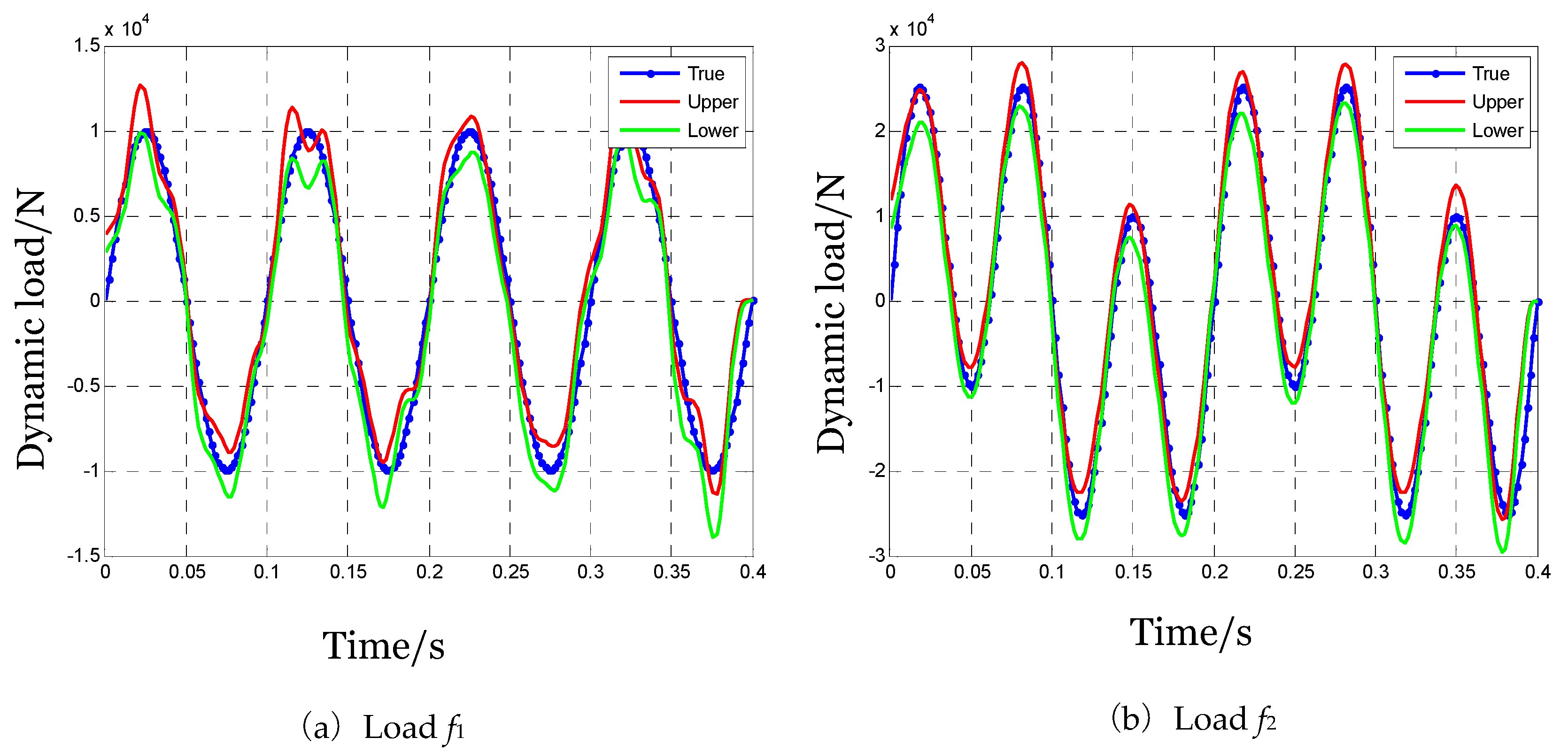
Figure 11.
Load bounds identified using the ellipsoid model under , .
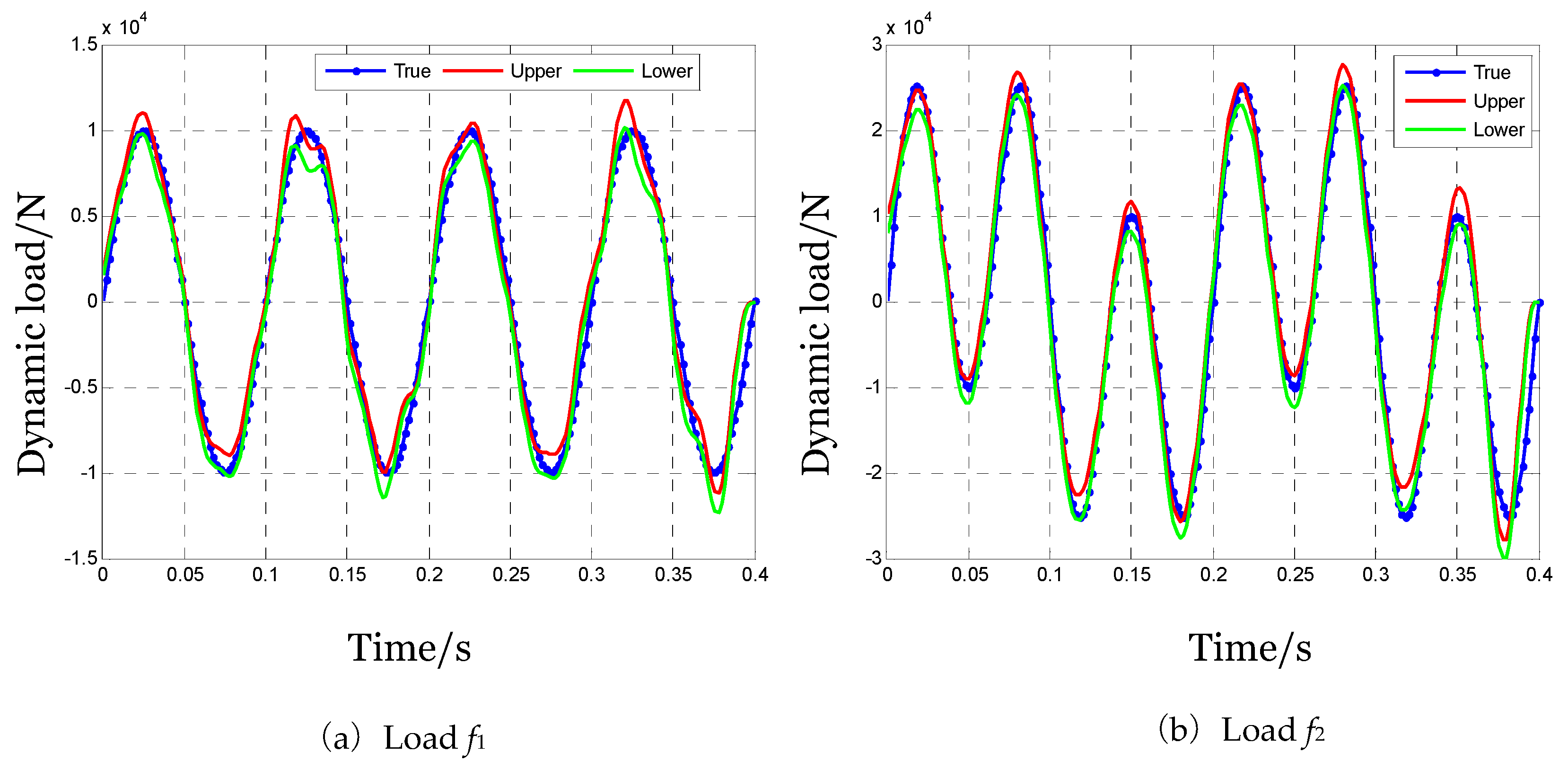
Figure 12.
Load bounds identified using the ellipsoid model under , .
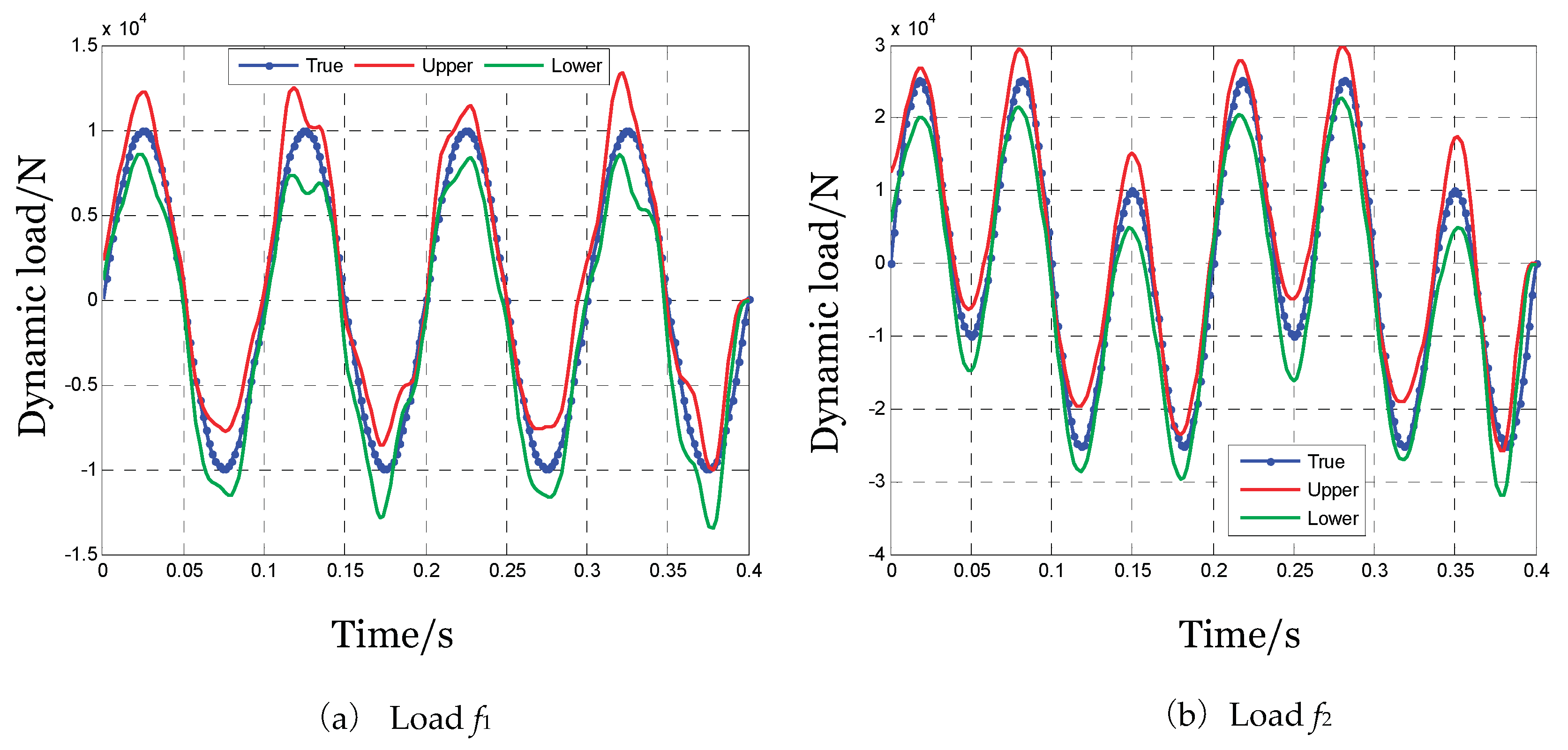

Table 1.
Comparison between proposed method and Monte Carlo simulation.
| Method | Maximum Boundary Error (%) | Average Boundary Error (%) | Computational Time (s) |
| Proposed Method | 4.32 | 2.15 | 156 |
| Monte Carlo Simulation | 3.87 | 1.92 | 2847 |
Disclaimer/Publisher’s Note: The statements, opinions and data contained in all publications are solely those of the individual author(s) and contributor(s) and not of MDPI and/or the editor(s). MDPI and/or the editor(s) disclaim responsibility for any injury to people or property resulting from any ideas, methods, instructions or products referred to in the content. |
© 2025 by the authors. Licensee MDPI, Basel, Switzerland. This article is an open access article distributed under the terms and conditions of the Creative Commons Attribution (CC BY) license (http://creativecommons.org/licenses/by/4.0/).
Copyright: This open access article is published under a Creative Commons CC BY 4.0 license, which permit the free download, distribution, and reuse, provided that the author and preprint are cited in any reuse.


