Orientational Phase Transitions

1. Phase Transitions

1.1. Introduction

The definition of the phase (phase state) concept is based on the symmetry of the crystal, both spatial and magnetic. Phase transitions (PT), as a rule, occur with a change in the crystal’s symmetry. Thus, during structural phase transitions, the crystal before and after the transition has a different crystal structure. For small atomic displacements, some symmetry elements are lost, and symmetry is lowered (distortional PT); however, there is a subgroup relationship between the low-symmetry (usually low-temperature) and high-symmetry (usually high-temperature) phases. For large atomic displacements during PT, a subgroup relationship between the symmetry groups of the two phases may not exist (reconstructive PT). In both cases, we are dealing with PTs of the displacement type. A structural PT can also occur as an "order-disorder" transition (atomic ordering in alloys like CuZn...). Classical objects for the physics of PT are magnetic materials, which is primarily due to the diversity of observed magnetic structures. Among magnetic PTs, the best-known are "order-disorder" type transitions at Curie ($T_C$ – ferromagnetic ordering temperature) and Néel ($T_N$ – antiferromagnetic ordering temperature) points. A common characteristic feature of such transitions is the appearance, for $T<T_C\left(T_N\right)$, of a non-zero average magnetic moment per atom. In other words, these PTs occur with a change in the magnitude of the average atomic magnetic moment. Among magnetic "order-disorder" type PTs, the so-called magnetic orientational PTs or spin-reorientation (SR) transitions are particularly distinguished. A characteristic feature of such transitions is a smooth or sharp change in the orientation (direction) of the atomic magnetic moments (spins).

Like other phase transitions, SR transitions can be spontaneous, i.e., occur solely under the influence of temperature change, or induced by an external magnetic field, electric field, or mechanical stress. A number of authors include in the concept of an SR transition only transitions with a change in magnetic state (orientation of magnetic moments) but without a change in the magnetic structure (ferro-, ferri-, or antiferromagnetic). In many cases, the concept of an SR transition is extended to all transitions accompanied by a change in the orientation of the magnetic moments of atoms or magnetic sublattices in multi-sublattice magnets. In this case, SR transitions include such well-known magnetic ones as spin-flop (reorientation of sublattices in antiferromagnets in an external magnetic field), the Morin transition (ferro – antiferromagnet transition), the metamagnetic transition (antiferromagnet – ferromagnet transition in highly anisotropic materials in an external field).

A feature of orientational PTs is the wide applicability range of the simple Landau theory, which, unlike PTs at the Curie point, is valid up to temperatures differing from the transition temperature by an extremely small amount ${10}^{-6}÷{10}^{-8}$ K.

1.2. Elements of Landau Theory

In the thermodynamic description of PT, the order parameter $\eta$ introduced by L.D. Landau is of fundamental importance. This parameter always characterizes some new property that appears in the system as a result of a PT from the original phase where it was absent. In other words, the order parameter is zero in the original (high-symmetry) phase and non-zero in the new (low-symmetry) phase. Thus, during a 2nd order phase transition, a symmetry breaking of the system occurs.

In the general case, the parameter $\eta$ can be multi-component (e.g., two angles of magnetic moment orientation). Below we consider the simplest theory of spontaneous 2nd order PTs.

The thermodynamic potential is written as a polynomial including invariant combinations of the order parameter to various powers. For example, for a single-component parameter $\eta$:

$$\Phi \left(\eta \right)={\Phi }_0+A{\eta }^2+B{\eta }^4+\dots$$

(1)

A linear term in the expression for $\Phi \left(\eta \right)$ is absent because the condition for the energy minimum for the equilibrium of the new phase requires that

$${\displaystyle \frac{\partial \Phi }{\partial \eta }}=0,$$

(2)

including at the transition point itself ($\eta =0$). Along with the minimum condition (1.2), the condition for phase stability must be fulfilled

$${\left.{\displaystyle \frac{{\partial }^2\Phi }{\partial {\eta }^2}}\right|}_{\eta ={\eta }_0}>0,$$

(3)

Bellow we will only use terms with ${\eta }^2,{\eta }^4$. Depending on A and B parameters there are 4 cases for $\Phi \left(\eta \right)$ dependency (Figure 1).

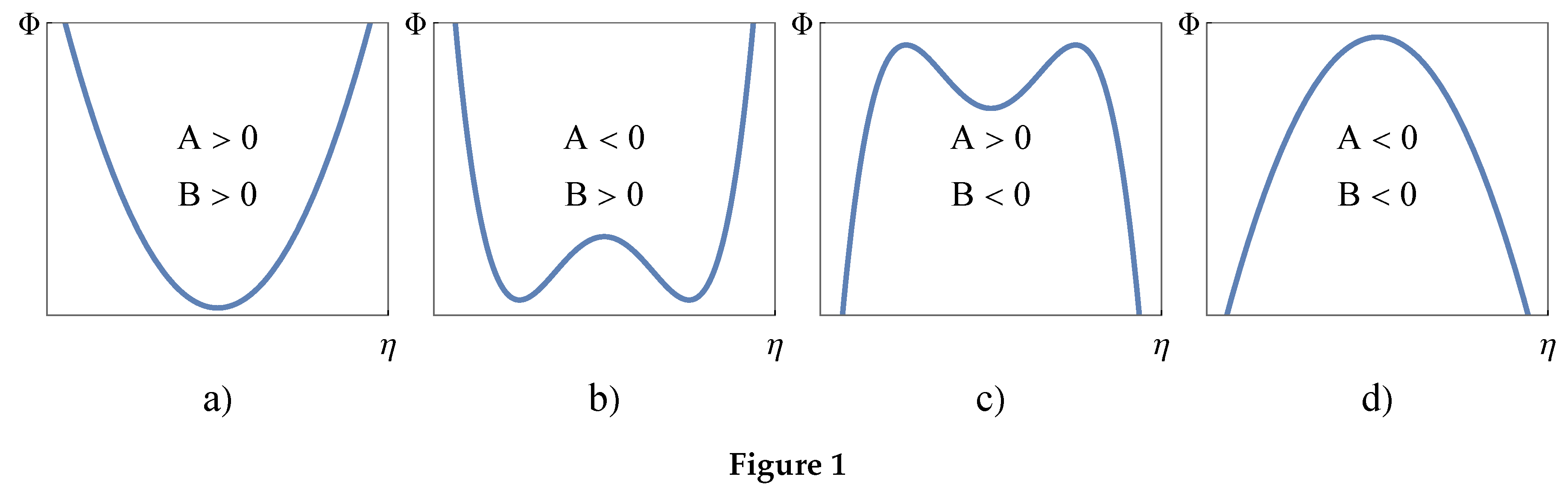
Case (d) is uninteresting because it does not correspond to any stable states. Case (c) corresponds to the existence of a metastable state. The most interesting are cases (a) and (b). In case (a), the energy minimum corresponds to $\eta =0$ (original phase); in case (b) — to $\eta \ne 0$ (new phase). During the transition from (a) to (b), the coefficient A changes sign. Since we are considering a spontaneous PT, the only reason for the change in A can be a change in temperature T. Expanding $A\left(T\right)$ near the transition point ($T=T_c$) in a Taylor series and keeping only the first (linear) term, we have

$$A=A_0(T-T_c).$$

(4)

We will consider the coefficient B to be constant hereafter: $B=\mathrm{const}$.

From the condition for the minimum of the thermodynamic potential, we find

$${\displaystyle \frac{\partial \Phi }{\partial \eta }}=(2A+4B{\eta }^2)\eta =0,$$

(5)

which gives two solutions:

(1)

$\eta =0$ for original phase;

(2)

${\eta }^2=-{\displaystyle \frac{A}{2B}}$ for new phase ($B>0$).

The stability condition gives

$${\displaystyle \frac{{\partial }^2\Phi }{\partial {\eta }^2}}=2A+12B{\eta }^2>0,$$

(6)

i.e., the original phase ($\eta =0$) is stable for $A>0$, and the new phase ($\eta \ne 0$) for $A<0$. In the new phase

$${\eta }^2=-{\displaystyle \frac{A}{2B}}=-{\displaystyle \frac{A_0}{2B}}(T-T_c),$$

(7)

or

$$\eta =\pm {\left[{\displaystyle \frac{A_0}{2B}}(T_c-T)\right]}^{{\displaystyle \frac{1}{2}}}.$$

(8)

The obtained temperature dependence of the order parameter near $T_c$ is characteristic of Landau theory.

Note also that in the low-symmetry phase, the parameter $\eta$ can be either positive or negative. This fact reflects the so-called Curie principle, according to which a dissymmetry appearing in a system must be present in the causes that give rise to it.

According to this principle, the symmetry of a crystal should not seem to change with temperature, since the latter is a scalar. This contradiction between the Curie principle and the aforementioned emergence of symmetry breaking during second-order phase transitions is resolved by the crystal breaking into domains with different signs of $\eta$ for $T<T_c$. The symmetry within each domain is lower than in the high-temperature phase; however, their arrangement in the crystal is determined by those symmetry elements that were lost during the phase transition, as a result of which the overall symmetry of the crystal remains unchanged.

1.3. Elements of Thermodynamics of Solids

In the thermodynamic description of solids, it is customary to introduce the so-called generalized thermodynamic forces (temperature T, electric E and magnetic H field, mechanical stress $\sigma$) and generalized thermodynamic coordinates (entropy S, electric displacement field D, magnetic flux density B, strain $\epsilon$).

The thermodynamic potential (TDP) $\Phi$, or Gibbs free energy, is a function of the form

$$\Phi =\mathcal{U}-TS-{\sigma }_{ij}{\epsilon }_{ij}-\dots =\mathcal{U}-X_i{x}_i,$$

(9)

where $\mathcal{U}$ is an internal energy, $X_i$ is a generalized force, $x_i$ is a generalized coordinate. The total differential of $\Phi$ is

$$d\Phi =-SdT-{\epsilon }_{ij}d{\sigma }_{ij}-\dots =-x_{i}d{X}_i,$$

(10)

since for the internal energy

$$d\mathcal{U}=TdS+{\sigma }_{ij}d{\epsilon }_{ij}+\dots =X_{i}d{x}_i.$$

(11)

If $\Phi$ is considered as a function of the generalized forces, then for the generalized coordinates we have

$$x_i=-{\displaystyle \frac{\partial \Phi }{\partial X_i}}.$$

(12)

Let us consider as the initial state one in which external forces are absent ($\mathbf{E}=0$, $\mathbf{H}=0$, $\sigma =0$, $T=T_0$). Expanding the generalized coordinates $x_i$ in a Taylor series, we obtain

$$x_i=-{\displaystyle \frac{\partial \Phi }{\partial X_i}}{|}_0-{\displaystyle \frac{{\partial }^2\Phi }{\partial X_i\partial X_j}}{|}_0{X}_j-\dots =-{\displaystyle \frac{\partial \Phi }{\partial X_i}}{|}_0+M_{ij}{X}_j-\dots .$$

(13)

Then the TDP can be represented as

$$\Phi ={\Phi }_0+{\displaystyle \frac{\partial \Phi }{\partial X_i}}{|}_0{X}_i+{\displaystyle \frac{1}{2}}{\displaystyle \frac{{\partial }^2\Phi }{\partial X_i\partial X_j}}{|}_0{X}_i{X}_j+\dots ={\Phi }_0+{\displaystyle \frac{\partial \Phi }{\partial X_i}}{|}_0{X}_i-{\displaystyle \frac{1}{2}}{M}_{ij}{X}_i{X}_j+\dots .$$

(14)

Most often, the second term in the expansion of $\Phi$ is absent (exceptions are crystals without spontaneous electric or magnetic polarization, nor spontaneous strain, and ferroelectrics, ferromagnets, and ferroelastics — crystals with spontaneous deformation). The tensors $M_{ij}=-{\partial }^2\Phi /\partial X_i\partial X_j{|}_0$ have the meaning of generalized susceptibilities, for example:

$$-{\displaystyle \frac{{\partial }^2\Phi }{\partial T^2}}{|}_0={\displaystyle \frac{C_p}{T}},$$

where $C_p$ is heat capacity at constant pressure;

$$-{\displaystyle \frac{{\partial }^2\Phi }{\partial E_i\partial E_j}}{|}_0={\epsilon }_{ij}$$

- dielectric susceptibility (permittivity);

$$-{\displaystyle \frac{{\partial }^2\Phi }{\partial E_i\partial T}}{|}_0=p_i^E$$

- pyroelectric coefficients;

$$-{\displaystyle \frac{{\partial }^2\Phi }{\partial H_i\partial H_j}}{|}_0={\mu }_{ij}$$

- magnetic susceptibility (permeability);

$$-{\displaystyle \frac{{\partial }^2\Phi }{\partial H_i\partial T}}{|}_0=p_i^M$$

- pyromagnetic coefficients;

$$-{\displaystyle \frac{{\partial }^2\Phi }{\partial {\sigma }_{ij}\partial {\sigma }_{kl}}}{|}_0=S_{ijkl}$$

- tensor of elastic compliances;

$$-{\displaystyle \frac{{\partial }^2\Phi }{\partial {\sigma }_{ij}\partial T}}{|}_0={\alpha }_{ij}^{\sigma }$$

- coefficients of thermal expansion (at constant stress);

$$-{\displaystyle \frac{{\partial }^2\Phi }{\partial E_i\partial {\sigma }_{jk}}}{|}_0=d_{ijk}^E$$

- piezoelectric coefficients;

$$-{\displaystyle \frac{{\partial }^2\Phi }{\partial H_i\partial {\sigma }_{jk}}}{|}_0=d_{ijk}^M$$

- piezomagnetic coefficients. The tensor M of generalized susceptibilities is symmetric: $M_{ij}=M_{ji},$ i.e., $M_{ij}$ determines both the change in the coordinate $x_i$ under the action of the force $X_j$, and vice versa, the change in $x_j$ under the action of $X_i$. Thus, for example, the pyromagnetic coefficient $p_i^M$ determines the change in magnetic induction with temperature and the change in entropy under the action of a magnetic field (the magnetocaloric effect). Incidentally, the magnetocaloric effect can be realized in two variants:

1. Isothermal process ($\Delta T=0$)

$$\Delta S=p_k^M{H}_k=({\mathbf{p}}^M·\mathbf{H}),$$

(15)

i.e., the crystal absorbs heat from the surroundings:

$$\Delta Q=T\Delta S=T({\mathbf{p}}^M·\mathbf{H}).$$

(16)

(It releases heat if ${\mathbf{p}}^M·\mathbf{H}<0$).

2. Adiabatic process (heat exchange with the surroundings is excluded, and $\Delta S=0$). In this case:

$$\Delta S=-{\displaystyle \frac{C_p}{T}}\Delta T+{\mathbf{p}}^M·\mathbf{H}=0,$$

(17)

and

$$\Delta T={\displaystyle \frac{T}{C_p}}({\mathbf{p}}^M·\Delta \mathbf{H}).$$

(18)

Considering that, as a rule, for paramagnets

$${\mathbf{p}}^M=-{\displaystyle \frac{{\partial }^2\Phi }{\partial T\partial \mathbf{H}}}{|}_0={\displaystyle \frac{\partial \mathbf{I}}{\partial T}}{|}_{\mathbf{H}}<0,$$

we arrive at the conclusion that the temperature decreases when the field is reduced (magnetic cooling).

1.4. Features of Generalized Susceptibilities Near a 2nd Order PT

In the general case, the TDP of a crystal is a function of the order parameter and thermodynamic forces $T,\mathbf{E},\mathbf{H},\sigma ,\dots$: $\Phi =\Phi (\eta ,T,\mathbf{E},\mathbf{H},\sigma )$.

Here, the order parameter is itself a function of the forces $(T,\mathbf{E},\mathbf{H},\sigma ,\dots )$ and is determined from the condition of the minimum of the TDP; in other words, the only independent variables in the TDP are the forces. It is completely obvious that the nature of phase transitions from the high-temperature phase should not change if the crystal is preliminarily subjected to any symmetry transformation that maps it onto itself. Consequently, the TDP used to describe a phase transition must be invariant under the transformations of the symmetry group of the high-temperature phase.

The expansion of the TDP near the PT point includes three types of terms of minimal degree in $\eta$ and X:

(1)

Terms of the type ${\eta }^2,{\eta }^4,\dots$;

(2)

Terms of the type $X_i{X}_j,\dots$;

(3)

Terms of the type $\eta X_i,{\eta }^2{X}_i,\dots ,\eta X_i,{\eta }^2{X}_i{X}_j$.

The order parameter is found from the condition of the minimum of the TDP:

$${\displaystyle \frac{\partial \Phi (T,X,\eta )}{\partial \eta }}{|}_{X=X_0}=0,{\displaystyle \frac{{\partial }^2\Phi (T,X,\eta )}{\partial {\eta }^2}}{|}_{X=X_0}>0,$$

(19)

where

$$\Phi ={\Phi }_0+A{\eta }^2+B{\eta }^4-{\displaystyle \frac{1}{2}}M{X}^2+N\eta X+K{\eta }^{2}X+\dots$$

(20)

(for simplicity, we restrict ourselves to only one force X). Below we analyze the PT, keeping in the TDP only the terms highlighted in (20).

1.4.1. Accounting for Terms of the Type $\eta X$ ($N\ne 0,K=0$)

The first of the TDP minimum conditions (19) in this case reduces to

$${\displaystyle \frac{\partial \Phi }{\partial \eta }}=2A\eta +4B{\eta }^3+NX=0.$$

(21)

Differentiating this equality with respect to X, we get

$$2A{\displaystyle \frac{\partial \eta }{\partial X}}+12B{\eta }^2{\displaystyle \frac{\partial \eta }{\partial X}}+N=0,$$

(22)

whence

$${\displaystyle \frac{\partial \eta }{\partial X}}=-{\displaystyle \frac{N}{2A+12B{\eta }^2}}=\left\{\begin{array}{cc}-{\displaystyle \frac{N}{2A}}\hfill & (\mathrm{high}-\mathrm{symmetry}\mathrm{phase}),\hfill \\ -{\displaystyle \frac{N}{2A+12B{\eta }^2}}\hfill & (\mathrm{low}-\mathrm{symmetry}\mathrm{phase}).\hfill \end{array}\right.$$

Let us find the generalized coordinate x:

$$x=-{\displaystyle \frac{d\Phi }{dX}}=-{\displaystyle \frac{\partial \Phi }{\partial X}}-{\displaystyle \frac{\partial \Phi }{\partial \eta }}{|}_X{\displaystyle \frac{\partial \eta }{\partial X}}=-{\displaystyle \frac{\partial \Phi }{\partial X}}{|}_{\eta },$$

(I.22)

since $\partial \Phi /\partial \eta {|}_X=0$. Thus, differentiating x in (20) with respect to X and using (21), we obtain

$$x=MX-N\eta .$$

(24)

Let us define the effective (renormalized) susceptibility $M_{\mathrm{eff}}$ as

$$M_{\mathrm{eff}}={\displaystyle \frac{\partial x}{\partial X}}=-{\displaystyle \frac{{\partial }^2\Phi }{\partial X^2}}=M+N{\displaystyle \frac{\partial \eta }{\partial X}}=$$

$$=M+\left\{\begin{array}{cc}{\displaystyle -\frac{N^2}{2A}}\hfill & \left(\mathrm{high}-\mathrm{symmetry}\mathrm{phase}\right),\hfill \\ {\displaystyle -\frac{N^2}{2A+12B{\eta }^2}}\hfill & \left(\mathrm{low}-\mathrm{symmetry}\mathrm{phase}\right).\hfill \end{array}\right.$$

Substituting ${\eta }^2=-A/2B$, we get

$$M_{\mathrm{eff}}=M+\left\{\begin{array}{cc}{\displaystyle -\frac{N^2}{2A}}\hfill & \left(\mathrm{high}-\mathrm{symmetry}\mathrm{phase}\right),\hfill \\ {\displaystyle +\frac{N^2}{4A}}\hfill & \left(\mathrm{low}-\mathrm{symmetry}\mathrm{phase}\right).\hfill \end{array}\right.$$

(25)

Considering that near $T\sim T_c$, $A=A_0(T-T_c)$ and $A_0>0$, we obtain

$$M_{\mathrm{eff}}=M_0+\left\{\begin{array}{cc}{\displaystyle -\frac{N^2}{2A_0}{\tau }^{-1},}\hfill & T>T_c,\hfill \\ {\displaystyle +\frac{N^2}{4A_0}{\left|\tau \right|}^{-1},}\hfill & T<T_c,\hfill \end{array}\right.$$

(26)

where $\tau =T-T_c$.

Thus, when terms of the type $\eta X$, linear in the order parameter and the force, are present in the TDP, the generalized susceptibility corresponding to the force X — generalized susceptibility has at $T_c$ a characteristic hyperbolic singularity.

1.4.2. Accounting for Terms of the Type ${\eta }^{2}X$ ($N=0,K\ne 0$)

In this case, the first of the minimum conditions (19) for the TDP reduces to

$${\displaystyle \frac{\partial \Phi }{\partial \eta }}=2\eta (A+KX)+4B{\eta }^3=0.$$

Differentiating with respect to X gives

$$2{\eta }^{\prime }(A+KX)+2K\eta +12B{\eta }^2{\eta }^{\prime }=0,$$

or

$${\eta }^{\prime }={\displaystyle \frac{\partial \eta }{\partial X}}=-{\displaystyle \frac{K\eta }{A+KX+6B{\eta }^2}}.$$

For the coordinate, we have

$$x=MX-K{\eta }^2,$$

and for the effective generalized susceptibility (at $X=0$)

$$M_{\mathrm{eff}}=M-2K\eta {\displaystyle \frac{\partial \eta }{\partial X}}=M+{\displaystyle \frac{2K^2{\eta }^2}{A+6B{\eta }^2}},$$

$$M_{\mathrm{eff}}=\left\{\begin{array}{cc}M,\hfill & T>T_c,\hfill \\ M+{\displaystyle \frac{K^2}{\left|A\right|}},\hfill & T<T_c,\hfill \end{array}\right.$$

(27)

taking into account that ${\eta }_0^2=-{\displaystyle \frac{A}{2B}}$.

Thus, if the TDP contains only terms of the type ${\eta }^{2}X$, which are quadratic in the order parameter but linear in the force X, then the corresponding generalized susceptibility experiences a jump at the same 2nd order PT point.

2. Spontaneous Orientational Phase Transitions

2.1. Orientational Phase Transitions in Uniaxial Magnets

Without an external magnetic field a thermodynamic potential (TDP) of an uniaxial magnet has the following form:

$$\Phi =K_1{sin}^2\theta +K_2{sin}^4\theta ,$$

(28)

where $K_1$ and $K_2$ are the first and second anisotropy constants, $\theta$ is the angle between the z-axis and a magnetic moment $\overrightarrow{M}$. The TDP minimum condition

$${\displaystyle \frac{\partial \Phi }{\partial \theta }}=sin2\theta \left(K_1+2K_2{sin}^2\theta \right)=0$$

(29)

gives us

$$\begin{array}{cc}\hfill \mathrm{I}.& sin2\theta =0,\mathrm{i}.\mathrm{e}.\mathrm{the}\mathrm{phases}{M}_{\left|\right|}(\theta =0)\mathrm{and}{M}_{\perp }(\theta =\pi /2)\hfill \\ \hfill \mathrm{II}.& {sin}^2\theta =-{\displaystyle \frac{K_1}{2K_2}},\mathrm{i}.\mathrm{e}.\mathrm{the}\mathrm{angular}\mathrm{phase}{M}_{>}.\hfill \end{array}$$

(30)

The thermodynamic stability condition of the phases

$${\displaystyle \frac{{\partial }^2\Phi }{\partial {\theta }^2}}=2cos2\theta \left(K_1+K_2{sin}^2\theta \right)+2K_2{sin}^{2}2\theta \ge 0$$

(31)

leads us to the following relations:

$$\begin{array}{cc}\hfill a)& K_1\ge 0\mathrm{for}\mathrm{the}{M}_{\left|\right|}-\mathrm{phase},\hfill \\ \hfill b)& K_1+2K_2\le 0\mathrm{for}\mathrm{the}{M}_{\perp }-\mathrm{phase},\hfill \\ \hfill c)& K_2\ge 0\mathrm{at}{K}_1\le 0\mathrm{and}{K}_1+2K_2\ge 0\mathrm{for}\mathrm{the}{M}_{>}-\mathrm{phase},\hfill \end{array}$$

(32)

which define a regions of the phase existence (Figure ).

The equality to zero in the relations (32) define lines of the stability loss (lability borders).

Values of the TDP in the different phases

$$\Phi \left(M_{\left|\right|}\right)=0;\Phi \left(M_{\perp }\right)=K_1+K_2;\Phi \left(M_{>}\right)={\displaystyle \frac{K_1^2}{4K_2}}$$

(33)

allow us to find the exact form of equations, which define the lines of the phase transitions:

$$\begin{array}{cc}\hfill a)& K_1+K_2=0,K_1\ge 0\left(M_{\left|\right|}\leftrightarrow M_{\perp }\right);\hfill \\ \hfill b)& K_1=0,K_2\ge 0\left(M_{\left|\right|}\leftrightarrow M_{>}\right);\hfill \\ \hfill c)& K_1+2K_2=0,K_1\le 0\left(M_{\perp }\leftrightarrow M_{>}\right).\hfill \end{array}$$

(34)

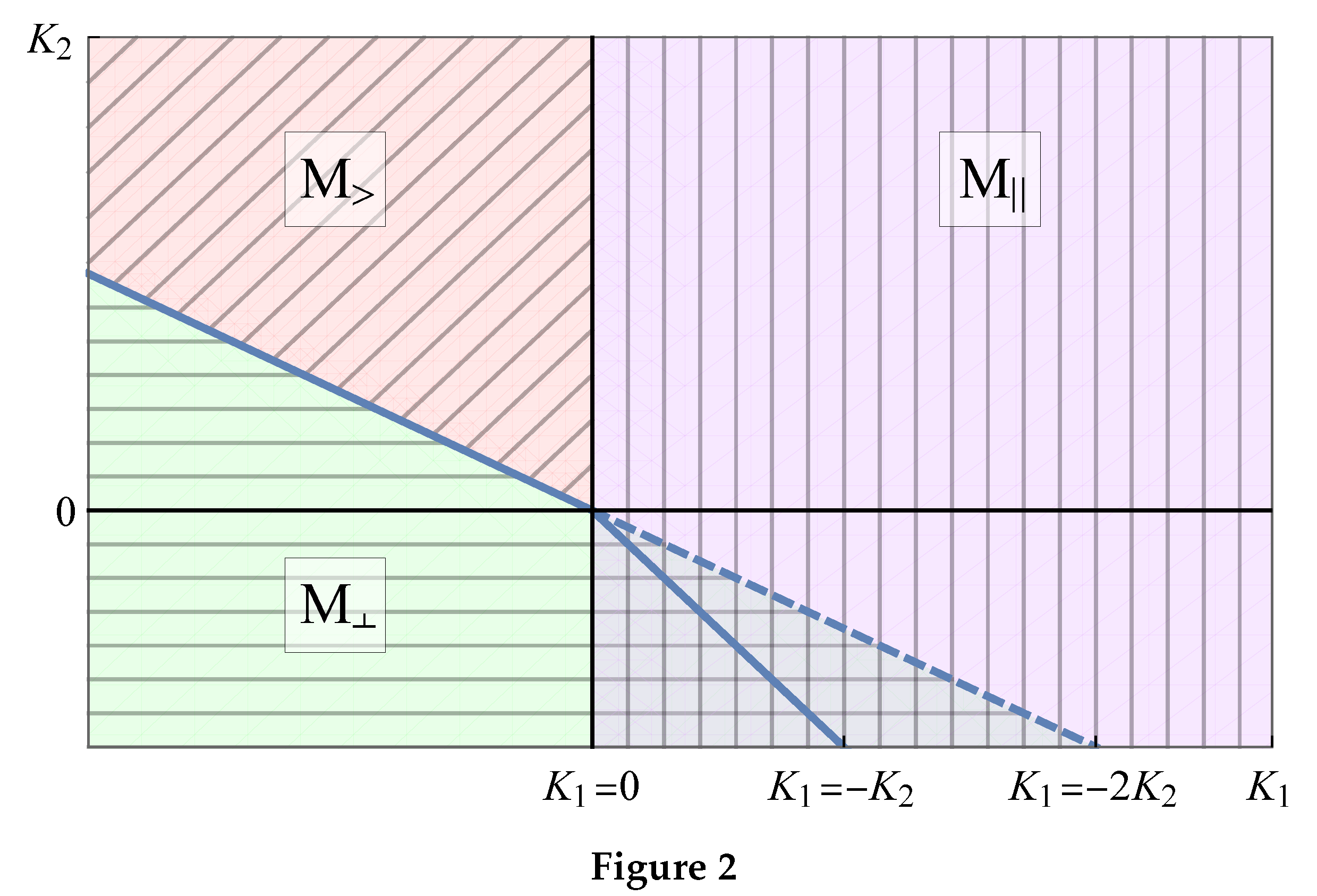
A magnetic phase diagram of the uniaxial magnet in the ($K_1$, $K_2$) coordinates shown in the Figure (the bold lines is the PT lines, the dashed lines represent the phase stability loss, or the lability borders).

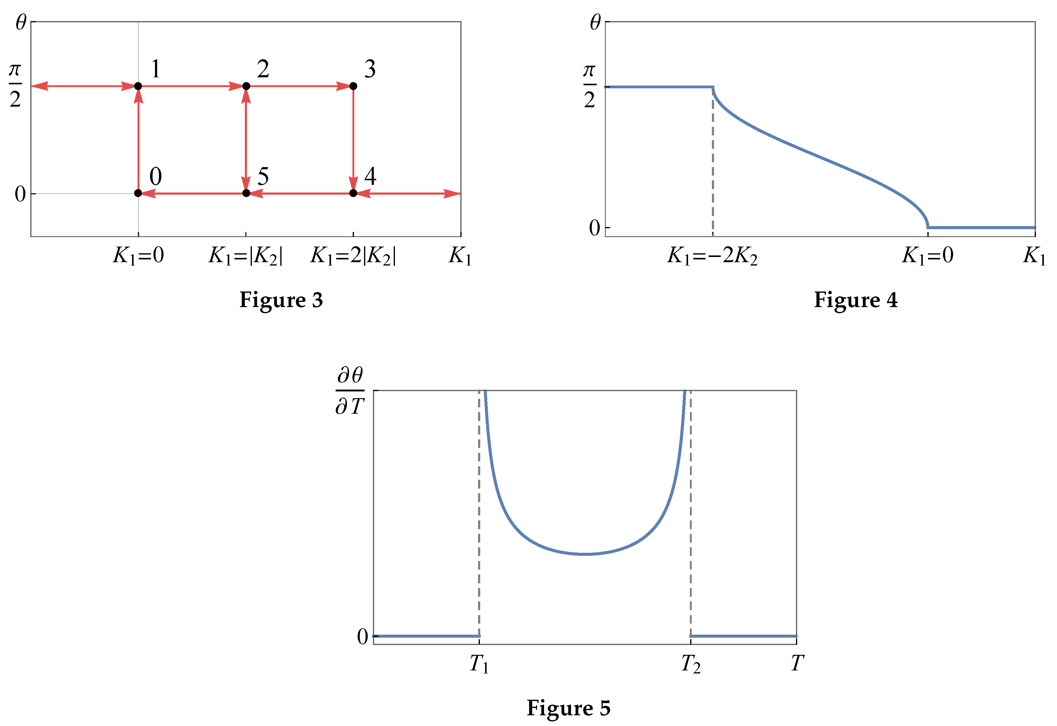
Let us pay attention to the presence of the phase coexistence areas ($M_{\left|\right|}$ and $M_{\perp }$) in the last case, which makes possible an appearance of a hysteresis and metastable states. A schematic dependence of the orientation angle of the vector $\overrightarrow{M}$ versus the anisotropy $K_1$ at $K_2=\mathrm{const}<0$ shown in the Figure 2. The sectors $2\to 3$ and $5\to 0$ correspond to the metastable states, which can appear in a single-domain sample. The transition $M_{\left|\right|}$ – $M_{\perp }$ could occur without hysteresis loops in the way $1\leftrightarrow 2\leftrightarrow 5\leftrightarrow 4$, because there are nucleus of the new phase in the domain borders of the old phase, which grows through the all crystal volume at $K_1$ changes with temperature.

A smooth $M_{\left|\right|}\to M_{\perp }$ orientational phase transition (OPT) realized with two second-order phase transition ($M_{\left|\right|}\to M_{>}$ and $M_{>}\to M_{\perp }$) through the intermediate angular phase $M_{>}$. Schematically the dependence of the orientation angle $\theta$ versus the $K_1$ at $K_2=\mathrm{const}>0$ given in the Figure 2. Note that in the angular phase the derivative

$${\displaystyle \frac{\partial \theta }{\partial K_1}}=-{\left(2K_{2}sin2\theta \right)}^{-1}$$

(35)

becomes infinity when $\theta =0$ and $\theta =\pi /2$. In a conventional OPT model it is considered that in the transition region $K_2=\mathrm{const}$ and $K_1$ is the linear function of temperature:

$$K_1\left(T\right)=-2K_2{\displaystyle \frac{T-T_2}{T_1-T_2}},$$

(36)

where $T_1$ and $T_2$ are the transition temperatures $M_{\perp }\leftrightarrow M_{>}$ and $M_{\left|\right|}\leftrightarrow M_{>}$ respectively. Then in the angular phase we have the following equations (with Figure ):

$$\begin{array}{cc}\hfill & {sin}^2\theta ={\displaystyle \frac{T-T_2}{T_1-T_2}},\hfill \\ \hfill {\displaystyle \frac{\partial \theta }{\partial T}}={\displaystyle \frac{1}{(T_1-T_2)sin2\theta }}=& {\displaystyle \frac{1}{2\sqrt{(T-T_1)(T_2-T)}}},T_1<T<T_2.\hfill \end{array}$$

(37)

In the uniaxial magnet the $M_{\left|\right|}$-phase could be named “easy-axis” phase, and the $M_{\perp }$-phase is “easy-plane”. In the angular phase $M_{>}$ takes place a cone of the easy-axes.

The given analysis could be applicable to an OPT in a certain crystallographic plane of a rhombic magnet.

2.2. Magnetic Part of a Heat Capacity at an OPT in Uniaxial Magnets

We use the well-known relation for a heat capacity at constant pressure

$$C_p=-T{\displaystyle \frac{{\partial }^2\Phi }{\partial T^2}},$$

(38)

and taking into account $\Phi =\Phi (\theta ,T)$ for an uniaxial magnet we get

$$C_p\left(m\right)=-T\left[{\left.{\displaystyle \frac{{\partial }^2\Phi }{\partial T^2}}\right|}_{\theta }+2{\displaystyle \frac{{\partial }^2\Phi }{\partial \theta \partial T}}·{\displaystyle \frac{\partial \theta }{\partial T}}+{\displaystyle \frac{{\partial }^2\Phi }{\partial {\theta }^2}}·{\left({\displaystyle \frac{\partial \theta }{\partial T}}\right)}^2\right],$$

(39)

where we used the TDP minimum condition $\partial \Phi /\partial \theta =0$.

From differentiating the minimum condition by temperature T we get

$${\displaystyle \frac{{\partial }^2\Phi }{\partial \theta \partial T}}+{\displaystyle \frac{{\partial }^2\Phi }{\partial {\theta }^2}}·{\displaystyle \frac{\partial \theta }{\partial T}}=0,$$

or

$${\displaystyle \frac{\partial \theta }{\partial T}}=-{\displaystyle \frac{{\Phi }_{\theta T}^{\prime \prime }}{{\Phi }_{\theta \theta }^{\prime \prime }}}.$$

(40)

Thus, we can rewrite the magnet part of the heat capacity in the form

$$\begin{array}{cc}\hfill C_p\left(m\right)& =-T\left[{\left.{\displaystyle \frac{{\partial }^2\Phi }{\partial T^2}}\right|}_{\theta }-{\left.{\displaystyle \frac{{\partial }^2\Phi }{\partial {\theta }^2}}\right|}_T{\left({\displaystyle \frac{\partial \theta }{\partial T}}\right)}^2\right]=\hfill \\ \hfill & =-T\left({\Phi }_{TT}^{\prime \prime }-{\displaystyle \frac{{\left({\Phi }_{\theta T}^{\prime \prime }\right)}^2}{{\Phi }_{\theta \theta }^{\prime \prime }}}\right)=C_p^{\prime }\left(m\right)+C_p^{\prime \prime }\left(m\right),\hfill \end{array}$$

(41)

where the second term is considered as the pure “orientational” contribution. With the account of (31) for ${\Phi }_{\theta \theta }^{\prime \prime }$ and

$${\Phi }_{\theta T}^{\prime \prime }=sin2\theta \left({\displaystyle \frac{\partial K_1}{\partial T}}+2{\displaystyle \frac{\partial K_2}{\partial T}}{sin}^2\theta \right)$$

(42)

we get the following equation for the orientational term in $C_p\left(m\right)$:

$$C_p^{\prime \prime }\left(m\right)=T{\displaystyle \frac{{sin}^{2}2\theta \left({\displaystyle \frac{\partial K_1}{\partial T}}+2{\displaystyle \frac{\partial K_2}{\partial T}}{sin}^2\theta \right)}{2cos2\theta \left(K_1+2K_2{sin}^2\theta \right)+2K_2{sin}^{2}2\theta }}=$$

$$=\left\{\begin{array}{cc}0,& M_{\left|\right|}-\mathrm{phase}\\ {\displaystyle \frac{T}{2K_2}}{\left({\displaystyle \frac{\partial K_1}{\partial T}}-{\displaystyle \frac{\partial K_2}{\partial T}}·{\displaystyle \frac{K_1}{K_2}}\right)}^2,& M_{>}-\mathrm{phase}\\ 0,& M_{\perp }-\mathrm{phase}\end{array}\right.$$

(43)

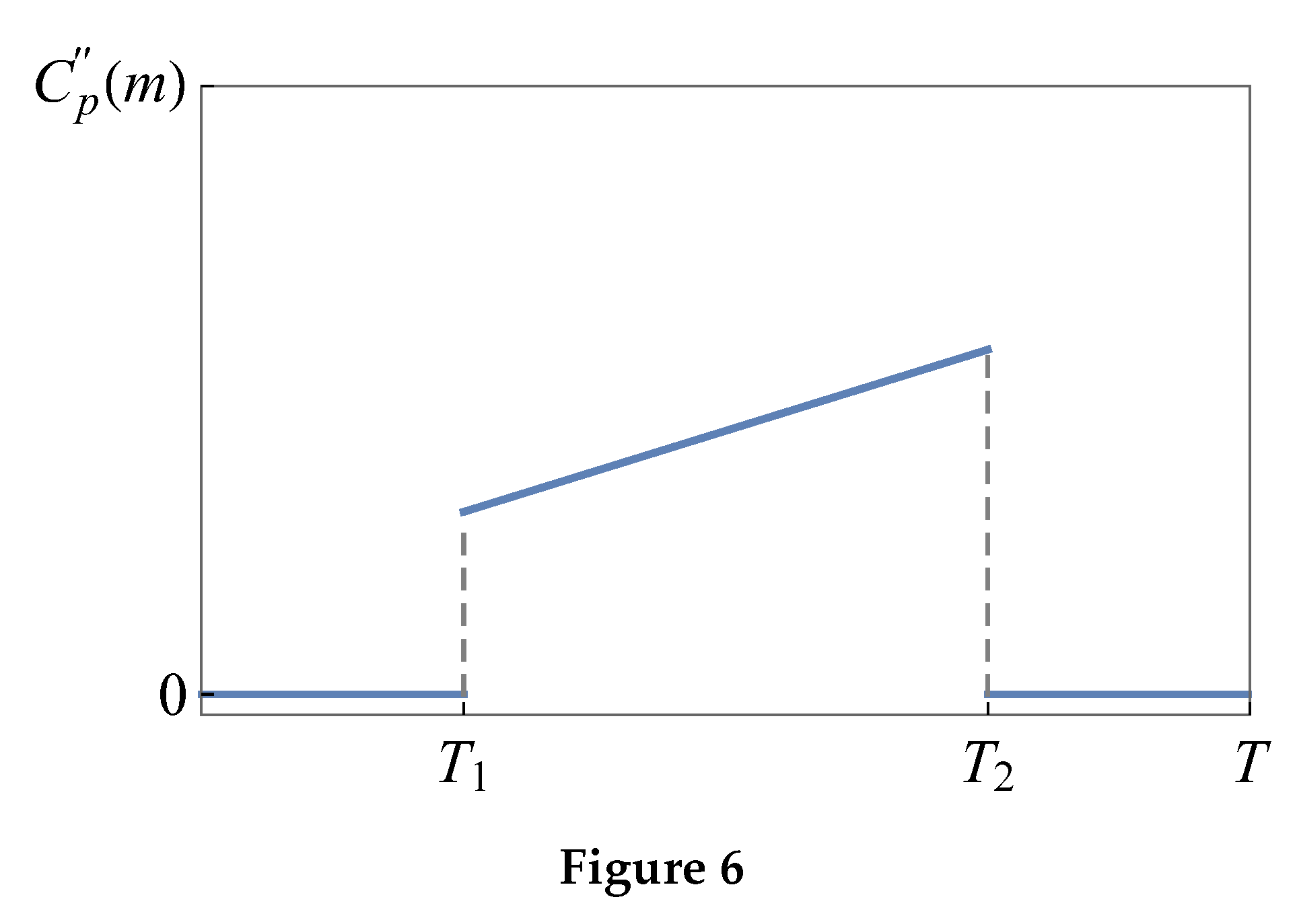
Assuming $K_2=\mathrm{const}$ and a linear temperature dependence of $K_1\left(T\right)$ like in (36) we have $C_p^{\prime }\left(m\right)=0$ and

$$C_p^{\prime \prime }\left(m\right)=\left\{\begin{array}{cc}0,& M_{\left|\right|}-\mathrm{phase}\\ {\displaystyle \frac{2K_{2}T}{{\left(T_1-T_2\right)}^2}},& M_{>}-\mathrm{phase}\\ 0,& M_{\perp }-\mathrm{phase}\end{array}\right.$$

(44)

A schematic temperature dependence of $C_p^{\prime \prime }\left(m\right)$ at a smooth OPT $M_{\left|\right|}\to M_{\perp }$ shown in the Figure .

2.3. Behavior Features of a Magnetic Susceptibility at an OPT

We write a TDP of an uniaxial or a rhombic ferromagnet (“plane” OPT) in an external magnetic field in the following form:

$$\Phi =K_1{sin}^2\theta +K_2{sin}^4\theta -\overrightarrow{m}\overrightarrow{H}-{\displaystyle \frac{1}{2}}\chi H^2.$$

(45)

At an analysis of the OPT $M_{\left|\right|}\to M_{>}$ the $sin\theta$, or the angle $\theta$ itself at the small rotations of $\overrightarrow{m}$, plays a role of an order parameter. Then we have

$$\Phi \simeq {\Phi }_0+K_1{\theta }^2+K_2{\theta }^4-m{H}_{\perp }\theta +{\displaystyle \frac{1}{2}}{m}_0{H}_{\left|\right|}{\theta }^2-{\displaystyle \frac{1}{2}}\chi H^2.$$

(46)

There is also a completely different behavior of the effective magnetic susceptibilities ${\chi }_{\perp }$ and ${\chi }_{\left|\right|}$, corresponding to $H_{\perp }$ and $H_{\left|\right|}$, i.e.

$$\begin{array}{cc}\hfill {\chi }_{\perp }=& {\chi }_{\perp }^0+\left\{2.3\begin{array}{cc}{\displaystyle \frac{m_0^2}{2K_1}},& M_{\left|\right|}-\mathrm{phase}\\ -{\displaystyle \frac{m_0^2}{4K_1}},& M_{>}-\mathrm{phase}\end{array}\right.\hfill \\ \hfill {\chi }_{\left|\right|}=& {\chi }_{\left|\right|}^0+\left\{\begin{array}{cc}0,& M_{\left|\right|}-\mathrm{phase}\\ {\displaystyle \frac{m_0^2}{8K_2}},& M_{>}-\mathrm{phase}\end{array}\right.\hfill \end{array}$$

(47)

At an analysis of the OPT $M_{>}\to M_{\perp }$ the angle ${\theta }^{\prime }=\pi /2-\theta$ could play a role of an order parameter, so at $\theta \sim \pi /2$

$$\Phi \simeq {\Phi }_0-(K_1+2K_2){\theta }^{\prime 2}+K_2{\theta }^{\prime 4}-m_0{H}_{\left|\right|}{\theta }^{\prime }+{\displaystyle \frac{1}{2}}{m}_0{H}_{\perp }{\theta }^{\prime 2}-{\displaystyle \frac{1}{2}}\chi H^2.$$

(48)

Thus, at the $M_{>}\to M_{\perp }$ transition we have

$$\begin{array}{cc}\hfill {\chi }_{\perp }=& {\chi }_{\perp }^0+\left\{\begin{array}{cc}{\displaystyle \frac{m_0^2}{8K_2}},& M_{>}-\mathrm{phase}\\ 0,& M_{\perp }-\mathrm{phase}\end{array}\right.\hfill \\ \hfill {\chi }_{\left|\right|}=& {\chi }_{\left|\right|}^0+\left\{\begin{array}{cc}{\displaystyle \frac{m_0^2}{4(K_1+2K_2)}},& M_{>}-\mathrm{phase}\\ -{\displaystyle \frac{m_0^2}{2(K_1+2K_2)}},& M_{\perp }-\mathrm{phase}\end{array}\right.\hfill \end{array}$$

(49)

Schematically the temperature behavior of the susceptibilities ${\chi }_{\left|\right|}$ and ${\chi }_{\perp }$ at the smooth OPT $M_{\left|\right|}\to M_{\perp }$ shown in the Figure 3. With the linear temperature dependence of $K_1\left(T\right)$ at the transition region and with $K_2=\mathrm{const}$ the susceptibility ${\chi }_{\perp }$ near the transition $M_{\left|\right|}\to M_{>}$ and ${\chi }_{\left|\right|}$ near the transition $M_{>}\to M_{\perp }$ have a characteristic for the Landau theory hyperbolic dependence:

$${\chi }_{\perp }\sim |T-T_2{|}^{-1},{\chi }_{\left|\right|}\sim {|T-T_1|}^{-1}.$$

(50)

2.4. Spatial Spin-Reorientation in Rhombic Magnets

Without external magnetic fields a magnetic anisotropy energy of rhombic magnets with a consideration of second and fourth order anisotropy has the following form:

$${\Phi }_{\mathrm{an}}=K_1{sin}^2\theta \left(1+\alpha {sin}^2\phi \right)+K_2{sin}^4\theta \left(1+\beta {sin}^2\phi +\gamma {sin}^4\phi \right),$$

(51)

where $\theta$, $\phi$ is the polar and azimuth orientation angles of a magnetization vector (or an antiferromagnetism vector). The constants $K_1$, $K_2$, $\alpha$, $\beta$, $\gamma$ can be connected with the first and the second anisotropy constants in the different crystallographic planes:

$$\begin{array}{cc}\hfill K_1\left(ac\right)=K_1;& K_1\left(bc\right)=K_1(1+\alpha );K_1\left(ab\right)=\alpha K_1+\beta K_2\hfill \\ \hfill K_2\left(ac\right)=K_2;& K_2\left(bc\right)=K_2(1+\beta +\gamma );K_2\left(ab\right)=\alpha K_2+\gamma K_2.\hfill \end{array}$$

(52)

As it is accepted for perovskites RFeO$3$ and RCrO$3$, let us select the magnetic configurations ${\Gamma }_1$, ${\Gamma }_2$, ${\Gamma }_4$, ${\Gamma }_{12}$, ${\Gamma }_{14}$, ${\Gamma }_{24}$, ${\Gamma }_{124}$, which are different by the antiferromagnetism vector orientation: ${\Gamma }_1(\overrightarrow{l}\left|\right|b)$, ${\Gamma }_2(\overrightarrow{l}\left|\right|c)$, ${\Gamma }_4(\overrightarrow{l}\left|\right|a)$ are the “clear” phases, ${\Gamma }_{12}(\overrightarrow{l}\perp a)$, ${\Gamma }_{14}(\overrightarrow{l}\perp c)$, ${\Gamma }_{24}(\overrightarrow{l}\perp b)$ are the angular phases and ${\Gamma }_{124}$ is the phase with a spatial orientation of $\overrightarrow{l}$. An equilibrium orientation of the vector $\overrightarrow{l}$ can be found from the minimization of ${\Phi }_{\mathrm{an}}$. A phase diagram of the rhombic magnet in coordinates $K_1$ and $K_1^{\prime }=\alpha K_1$ shown in the Figure at a condition of the positive second anisotropy constants in all of the crystallographic planes. The stability strips width of the phases ${\Gamma }_{24}$, ${\Gamma }_{12}$, ${\Gamma }_{14}$ are respectively $2K_2\left(ac\right)$, $\sqrt{2}{K}_2\left(bc\right)$, $2K_2\left(ab\right)$. The borderline between the phases ${\Gamma }_4$ and ${\Gamma }_{14}$ defined by the equation $K_1^{\prime }=-\beta K_2$ ($K_1\left(ab\right)=0$), and between the ${\Gamma }_2$ and ${\Gamma }_{12}$-phases by the equation $K_1^{\prime }=-K_1$ ($K_1\left(bc\right)=0$).

The triangle region in the center is the ${\Gamma }_{124}$ configuration stability region and it realizes only if $4\gamma -{\beta }^2>0$. Actually, at $4\gamma ={\beta }^2$ the triangle region degenerate into a segment, which is occur to be a borderline between two angular phases on the one side and the third angular phase on the other side (e.g. ${\Gamma }_{14}$, ${\Gamma }_{24}$, ${\Gamma }_{12}$). From the form of the diagram follows that the most possible transitions with the spatial orientation of the antiferromagnetism vector are complex cascading transitions like ${\Gamma }_4-{\Gamma }_{14}-{\Gamma }_{124}-{\Gamma }_{12}-{\Gamma }_1$, ${\Gamma }_2-{\Gamma }_{24}-{\Gamma }_{124}-{\Gamma }_{14}-{\Gamma }_1$, and etc., i.e. those scenarios, in which the transition to the ${\Gamma }_{124}$-phase and out from it goes through a intermediate angular phase.

2.5. Spin-Reorientation Transitions in Cubic Magnets

Without an external magnetic field a TDP of a cubic magnet has the form

$${\Phi }_{\mathrm{an}}=K_1\left({\alpha }_1^2{\alpha }_2^2+{\alpha }_2^2{\alpha }_3^2+{\alpha }_1^2{\alpha }_3^2\right)+K_2{\alpha }_1^2{\alpha }_2^2{\alpha }_3^2=$$

(53)

$$={\displaystyle \frac{1}{4}}\left(K_1{sin}^{2}2\theta +\left(K_1+K_2{cos}^2\theta \right){sin}^4\theta {cos}^{2}2\phi \right),$$

where ${\alpha }_i$ are the direction cosines of the magnetic moment vector $\overrightarrow{M}$ (or the antiferromagnetism vector in the cubic antiferromagnet), $\theta$, $\phi$ are the polar and azimuth angles of this vector orientation, $K_1$ and $K_2$ are the first and second anisotropy constants.

From minimizing (53) on $\theta$ and $\phi$ we find that minimum of the TDP realizes only when the vector $\overrightarrow{M}$ oriented along one of the three main crystallographic directions $\left[100\right]$, $\left[110\right]$ and $\left[111\right]$:

$$\begin{array}{cc}\hfill \overrightarrow{M}\left|\right|\left[100\right]& \mathrm{at}{K}_1\ge 0,\hfill \\ \hfill \overrightarrow{M}\left|\right|\left[110\right]& \mathrm{at}0\ge K_1\ge -\frac{1}{2}{K}_2,\hfill \\ \hfill \overrightarrow{M}\left|\right|\left[111\right]& \mathrm{at}{K}_1\le -\frac{1}{3}{K}_2.\hfill \end{array}$$

(54)

The equalities in the equations (54) correspond to the lines of the phases stability loss and, as it seen from (54), there is regions of the $K_1$ and $K_2$ magnitudes at which there is coexistence of the different phases. Comparing the TDP values we could find lines of the phase transitions:

$$\begin{array}{cc}\hfill {\Phi }_{\left[100\right]}={\Phi }_{\left[110\right]}& \mathrm{at}{K}_1=0,K_2\ge 0,\hfill \\ \hfill {\Phi }_{\left[110\right]}={\Phi }_{\left[111\right]}& \mathrm{at}9K_1+4K_2=0,K_1\le 0,\hfill \\ \hfill {\Phi }_{\left[111\right]}={\Phi }_{\left[100\right]}& \mathrm{at}9K_1+K_2=0,K_1\ge 0.\hfill \end{array}$$

(55)

The phase transitions in the cubic magnet with considering only two anisotropy constants $K_1$ and $K_2$ occur sharply at the absence of external magnetic fields, i.e. the spin-reorientation is a first order phase transition.

2.6. SR Peculiarities in Magnets with a Fluctuating Magnetic Anisotropy

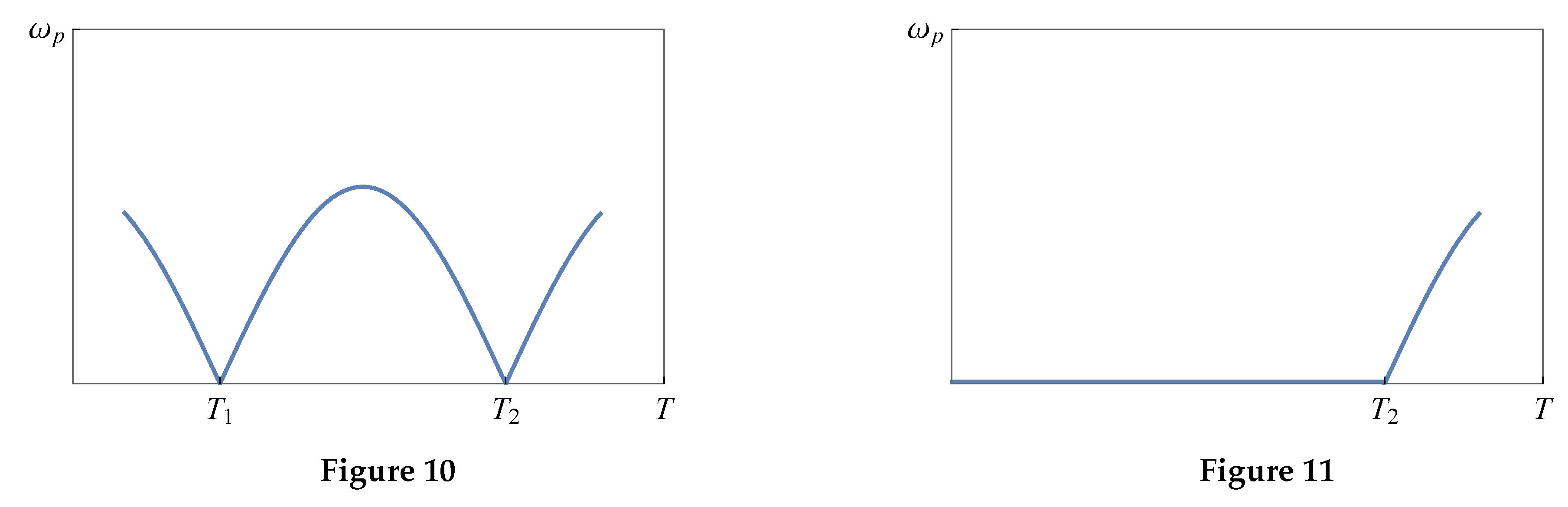
Compounds with a second order fluctuating magnetic anisotropy (i.e. many of disordered magnets, as well as compounds with substitution, containing ions with a different contribution to the magnetic anisotropy energy: R the eigenfrequency of the order parameter, when approaching the transition temperature from the high-symmetry phase, goes to zero and keeps equal to zero at the low-symmetry phase (Figure 5). This soft mode called a “Goldstone mode”.

3. Orientational Phase Transitions Induced by External Magnetic Fields

3.1. Uniaxial Ferromagnets

Consider an uniaxial ferromagnet with an easy-axis in parallel to the z-axis in an external magnetic field in a basal plane. A thermodynamic potential in this case has the following form

$$\Phi =K_1{sin}^2\theta +K_2{sin}^4\theta -m_{0}Hsin\theta ,(K_1>0),$$

(69)

where $m_0$ is the saturation magnetic moment. Equilibrium directions $\overrightarrow{m}$ can be determined from the condition

$${\displaystyle \frac{\partial \Phi }{\partial \theta }}=sin2\theta \left(K_1+2K_2{sin}^2\theta \right)-m_{0}Hcos\theta =0,$$

(70)

which gives us two phases:

a)

the “high-field” phase: $\theta =\pi /2$, $cos\theta =0$;

b)

the angular phase: $\theta \ne \pi /2$, $sin\theta \left(K_1+2K_2{sin}^2\theta \right)-m_{0}H=0$.

The last equation determine the magnetization curve in the angular phase if we consider $sin\theta =m_{\perp }/m_0=\mu$:

$$H={\displaystyle \frac{1}{m_0}}\left(2K_1\mu +4K_2{\mu }^3\right).$$

(71)

From the condition ${\displaystyle \frac{{\partial }^2\Phi }{\partial {\theta }^2}}>0$ at $cos\theta =0$ we can find the high-field phase stability region:

$$H\ge {\displaystyle \frac{2K_1+4K_2}{m_0}}=H_1$$

(72)

(the equality corresponds to the magnetic field at which the phase loses its stability). The stability region of the angular phase can be easily determined if we consider $\Phi$ in the form

$$\Phi =K_1{\mu }^2+K_2{\mu }^4-m_{0}H\mu .$$

(73)

In this case

$${\displaystyle \frac{\partial \Phi }{\partial \mu }}=2K_1\mu +4K_2{\mu }^3-m_{0}H=0$$

(74)

and

$${\displaystyle \frac{{\partial }^2\Phi }{\partial {\mu }^2}}=2K_1+12K_2{\mu }^2>0.$$

(75)

At $K_2\ge 0$ the angular phase stable for any $\mu$: $0\le \mu \le 1$, so the orientational phase transition from the angular phase into the high-field phase will always be a second-order phase transition with the critical field $H_1$ (Figure 6), at which the phase stability loss occurs and the values of the thermodynamic potentials equalize. At $K_2>0$ the angular phase loses stability at

$${\mu }^2\ge -{\displaystyle \frac{K_1}{6K_2}},$$

(76)

which corresponds to the value of the magnetic field

$$H\ge {\displaystyle \frac{4}{3}}{\displaystyle \frac{K_1}{m_0}}\sqrt{-{\displaystyle \frac{K_1}{6K_2}}}=H_2\ge H_1.$$

(77)

The field $H_2$ of the stability loss of the angular phase corresponds to a point on the magnetization curve, in which

$$\partial H/\partial \mu =0.$$

The TDP of the angular and high-field phases match up at $H=H_{\mathrm{crit}}$, which can be determined by the equation

$$K_1{\mu }^2+K_2{\mu }^4-m_0\mu H_{\mathrm{crit}}=K_1+K_2-m_0{H}_{\mathrm{crit}},$$

at

$$H_{\mathrm{crit}}={\displaystyle \frac{1}{m_0}}\left(2K_1\mu +4K_2{\mu }^3\right).$$

(78)

The solution of these equations gives us

$$H_{\mathrm{crit}}={\displaystyle \frac{2K_2}{27m_0}}\left(9{\displaystyle \frac{K_1}{K_2}}+10+\left(2+3{\displaystyle \frac{K_1}{K_2}}\right)\sqrt{-2-3{\displaystyle \frac{K_1}{K_2}}}\right),H_1\le H_{\mathrm{crit}}\le H_2.$$

(79)

Thus, at $K_2>0$ the transition from the angular phase into the high-field phase is a first-order phase transition.

Two different options of magnetization curves in a hard direction of the uniaxial ferromagnet shown in the Figure 6.

There is regions at $K_2>0$ in the magnetization curve corresponding to metastable states, which leads to hysteresis in single-domain samples. In multi-domain samples a hysteresis-free option of the first-order transition is possible.

All of the results above can be used for the analysis of a transition from the easy-plane phase $\overrightarrow{m}\perp z$ into the easy-axis phase $\overrightarrow{m}\left|\right|z$ at $\overrightarrow{H}\left|\right|z$. For this analysis the replacement $K_1\to -K_1-2K_2$ is needed in all of the expressions for the critical fields.

3.2. Anisotropic Antiferromagnets. “Spin-Flop” Transitions

An interaction energy of an antiferromagnet with an external magnetic field can be determined in the following form:

$${\Phi }_H=-{\displaystyle \frac{1}{2}}{\chi }_{\perp }{H}^2+{\displaystyle \frac{1}{2}}\left({\chi }_{\perp }-{\chi }_{\left|\right|}\right){\left(\overrightarrow{l}·\overrightarrow{H}\right)}^2,$$

(80)

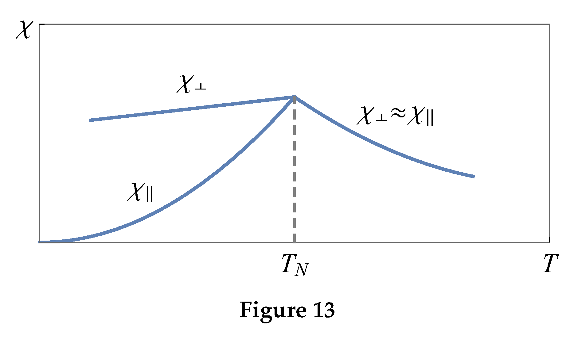
where $\overrightarrow{l}$ is the normalized antiferromagnetism vector ($2M_0\overrightarrow{l}={\overrightarrow{M}}_1-{\overrightarrow{M}}_2$ where ${\overrightarrow{M}}_{1,2}$ are the magnetization of the sublattices, $M_0=|{\overrightarrow{M}}_1|=|{\overrightarrow{M}}_2|$); ${\chi }_{\perp }$ is the perpendicular susceptibility (susceptibility at $\overrightarrow{H}\perp \overrightarrow{l}$), ${\chi }_{\left|\right|}$ is the parallel susceptibility (susceptibility at $\overrightarrow{H}\left|\right|\overrightarrow{l}$).

A characteristic temperature dependence of ${\chi }_{\perp }$ and ${\chi }_{\left|\right|}$ for weakly anisotropic antiferromagnets like MnF$2$ shown in the Figure .

In the transverse phase ($\overrightarrow{l}\perp \overrightarrow{H}$) of the antiferromagnet the Zeeman energy is less by ${\displaystyle \frac{1}{2}}\left({\chi }_{\perp }·{\chi }_{\left|\right|}\right)H^2$ than in the longitudinal phase ($\overrightarrow{l}\left|\right|\overrightarrow{H}$).

Let us consider a rhombic anisotropic antiferromagnet in external magnetic fields oriented along one of the crystallographic axes, e.g. z-axis. A TDP, which is describing rotation processes of $\overrightarrow{l}$ in one of the planes, will has the following form:

$$\begin{array}{cc}\hfill \Phi =& K_1{sin}^2\theta +K_2{sin}^4\theta -{\displaystyle \frac{1}{2}}{\chi }_{\perp }{H}^2+{\displaystyle \frac{1}{2}}\left({\chi }_{\perp }-{\chi }_{\left|\right|}\right)H^2{cos}^2\theta \hfill \\ \hfill =& \left[K_1-{\displaystyle \frac{1}{2}}\left({\chi }_{\perp }-{\chi }_{\left|\right|}\right)H^2\right]{sin}^2\theta +K_2{sin}^4\theta -{\displaystyle \frac{1}{2}}{\chi }_{\left|\right|}{H}^2,\hfill \end{array}$$

(81)

where $\theta$ is the angle between the z-axis and the vector $\overrightarrow{l}$.

Obviously, that taking into account the external magnetic field in this case leads to a renormalization of the first anisotropy constant. Thus, the analysis of the antiferromagnet behavior in the field can be based on the Section 2.1, in particular the phase diagram on the Figure .

At $K_2>0$ and the initial phase $\overrightarrow{l}\left|\right|z$ the inclusion of the external magnetic field $\overrightarrow{H}\left|\right|z$ leads to a “spin-flop” transition from the longitudinal phase $\overrightarrow{l}\left|\right|\overrightarrow{H}$ into the transverse phase $\overrightarrow{l}\perp \overrightarrow{H}$, which is starting at

$$H_{\left|\right|}=\sqrt{{\displaystyle \frac{2K_1}{{\chi }_{\perp }-{\chi }_{\left|\right|}}}},$$

(82)

as a second order phase transition (the transition into the angular phase), and ending at

$$H_{\perp }=\sqrt{{\displaystyle \frac{2K_1+4K_2}{{\chi }_{\perp }-{\chi }_{\left|\right|}}}}$$

(83)

also, as a second order phase transition (the transition from the angular phase into transverse phase).

At $K_2\le 0$ and $K_1>2\left|K_2\right|$ the initial longitudinal phase $\overrightarrow{l}\left|\right|\overrightarrow{H}$ loses the stability at $H_{\left|\right|}$, and the transverse phase became stable at $H=H_{\perp }$ ($H_{\perp }<H_{\left|\right|}$). Thus, in the region of fields $H_{\perp }<H<H_{\left|\right|}$ the longitudinal and transverse phases can coexist. Equality of the thermodynamic potentials of both phases takes place at $H=H_{\mathrm{crit}}=\sqrt{{\displaystyle \frac{2K_1+2K_2}{{\chi }_{\perp }-{\chi }_{\left|\right|}}}}$, and $H_{\perp }<H_{\mathrm{crit}}<H_{\left|\right|}$.

In an external magnetic field, which is exceeded the maximum of the critical fields $H_{\perp }$, $H_{\left|\right|}$, $H_{\mathrm{crit}}$, gradual “contraction” of the magnetic moments of the sublattices 1 and 2 to the direction of the magnetic field H occurs. So, in the sufficiently large magnetic field ($H\approx H_E$ for the weakly anisotropic antiferromagnets, $H_E={\displaystyle \frac{2m_0}{{\chi }_{\perp }}}$ is the exchange field) a ferromagnetic structure ${\overrightarrow{M}}_1\left|\right|{\overrightarrow{M}}_2\left|\right|H$ is realized.

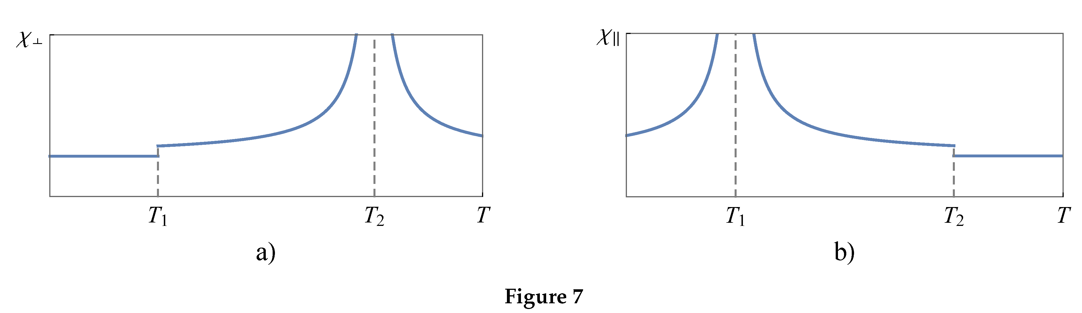
Schematically a magnetization curve of the antiferromagnet in our case shown in the Figure 7. The magnetic susceptibility on the region $0\le H\le H_{\left|\right|}$ (Figure 7a) or $0\le H\le H_{\perp }$ (Figure 7b) matches with ${\chi }_{\left|\right|}$, and on the region $H_{\left|\right|}\le H\le H_E$ it matches with ${\chi }_{\perp }$. On the region $H_{\left|\right|}\le H\le H_{\perp }$ (Figure 7a) the susceptibility has a “rotational” character:

$${\chi }_{\mathrm{rot}}={\displaystyle \frac{\partial m}{\partial H}}={\chi }_{\perp }-\left({\chi }_{\perp }-{\chi }_{\left|\right|}\right)\left({cos}^2\theta -{\displaystyle \frac{2H^2}{H_{\perp }^2-H_{\left|\right|}^2}}\right),$$

(84)

where we used the following relations:

$$m={\chi }_{\perp }H-\left({\chi }_{\perp }-{\chi }_{\left|\right|}\right){cos}^2\theta ·H,$$

(85)

$${\displaystyle \frac{\partial \theta }{\partial H}}={\displaystyle \frac{2H}{\left(H_{\perp }^2-H_{\left|\right|}^2\right)sin2\theta }}.$$

(86)

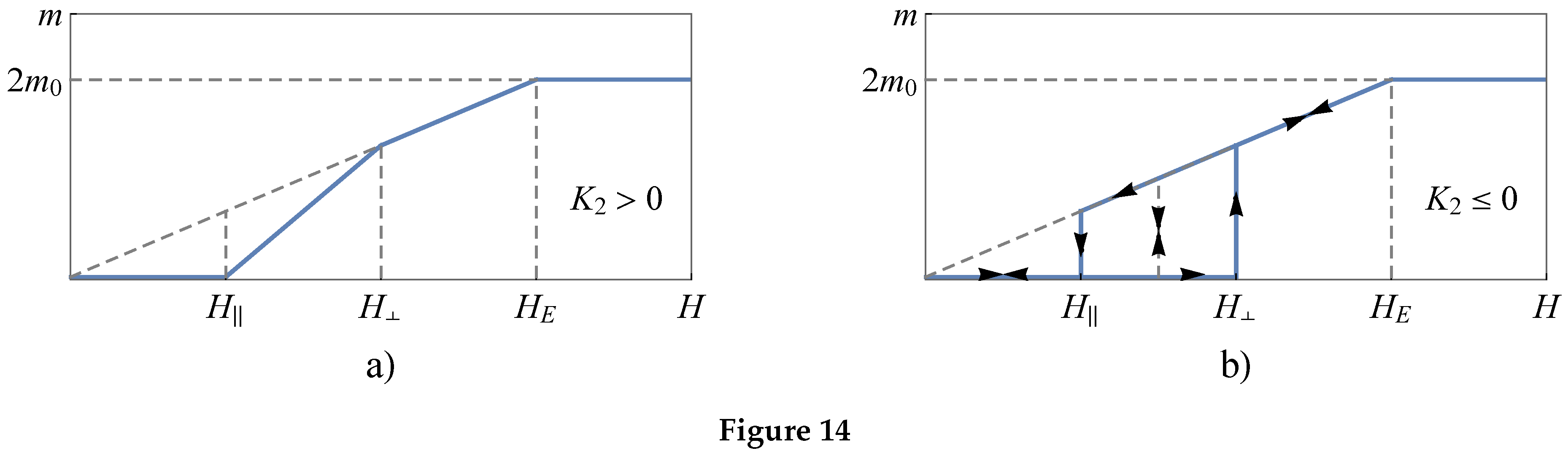
Let us pay attention to that $\partial \theta /\partial H\to \infty$ at $H\to H_{\left|\right|}$ from the right and at $H\to H_{\perp }$ from the left. At ${\chi }_{\perp }\gg {\chi }_{\left|\right|}$ (low temperature) and $\left(H_{\perp }-H_{\left|\right|}\right)\ll H_{\left|\right|}$ ($K_2\ll K_1$) the rotational susceptibility

$${\chi }_{\mathrm{rot}}\approx {\displaystyle \frac{H_{\left|\right|}}{H_{\perp }-H_{\left|\right|}}}{\chi }_{\perp }$$

(87)

can significantly exceed ${\chi }_{\perp }$.

3.3. Metamagnetic Transitions in High-Anisotropy Magnets

Considering the “spin-flop” transitions we implicitly assumed that a magnetic anisotropy energy is small in comparison with an exchange energy. There is, actually, a wide enough class of high-anisotropy magnets, which has the anisotropy energy comparable with the exchange energy, or even exceeds it. For a research of the peculiarities of orientational transitions induced by a magnetic field in such systems we restrict ourselves with $K_2=0$ case, and also with the region of sufficiently low temperatures, at which ${\chi }_{\left|\right|}\approx 0$ in antiferromagnets.

A model thermodynamic potential for the analysis of the orientational phase transition in the certain plane can be determined in the following form:

$$\begin{array}{cc}\hfill \Phi & =K_1\left({sin}^2{\theta }_1+{sin}^2{\theta }_2\right)+I{M}_0^{2}cos\left({\theta }_1-{\theta }_2\right)\hfill \\ \hfill & -M_{0}H\left(cos\left({\theta }_H-{\theta }_1\right)+cos\left({\theta }_H-{\theta }_2\right)\right),\hfill \end{array}$$

(88)

where I is the exchange constant, ${\theta }_{1,2}$ are the orientation angle of sublattices magnetic moments, ${\theta }_H$ is the orientation angle of the external magnetic field $\overrightarrow{H}$.

A minimization of the TDP in the magnetic field H, which is directed along the anisotropy axis (${\theta }_H=0$), gives us three equilibrium phases:

$$\begin{array}{ccc}\hfill 1.& {\theta }_1=0;{\theta }_2=\pi \hfill & \hfill (\mathrm{antiferromagnet}\mathrm{phase}),\\ \hfill 2.& {\theta }_1=-{\theta }_2\hfill & \hfill (\mathrm{phase}\mathrm{with}\mathrm{the}\mathrm{flipped}\mathrm{sublattices}),\\ \hfill 3.& {\theta }_1={\theta }_2=0\hfill & \hfill (\mathrm{ferromagnet}\mathrm{phase}).\end{array}$$

A research of the stability of this structures shows that the antiparallel ordering of the magnetic moments ${\theta }_1=0$, ${\theta }_2=\pi$ exist in the region

$$0<H<\sqrt{\left(2H_E+H_A\right)H_A}=H_c,$$

(89)

where $H_A=2K_1/M_0$, $H_E=I{M}_0$ are the anisotropy and the exchange field respectively. The second state ${\theta }_1=-{\theta }_2$ with the flipped lattices is stable in the region

$$H_c^{\prime }=\sqrt{{\displaystyle \frac{{\left(2H_E-H_A\right)}^2{H}_A}{2H_E+H_A}}}\le H\le H_c.$$

(90)

The magnetic fields $H_c^{\prime }$ and $H_c$ are the analogues of $H_{\perp }$ and $H_{\left|\right|}$ for the weakly anisotropic antiferromagnet (Figure 7b). The existing of overlapping phases witness about a possibility of hysteresis.

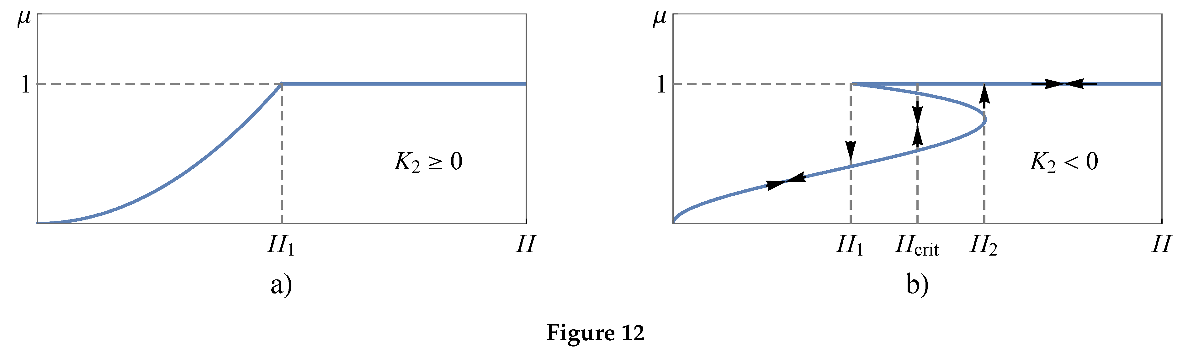
The state with the flipped sublattices at the increasing of the magnetic field smoothly transit into a “ferromagnet” state ${\theta }_1={\theta }_2=0$ in the magnetic field $H_{SF}=2H_E-H_A$.

With the increasing of the anisotropy constant, or the anisotropy field $H_A$, the magnitude of the magnetic field $H_{SF}$ decreases, but the magnitude of the magnetic field $H_c$ increases. With this the stability regions of the antiferromagnet phase (${\theta }_1=0$, ${\theta }_2=\pi$) and ferromagnet phase (${\theta }_1={\theta }_2=0$) expand, and simultaneously the stability region of the angular phase (${\theta }_1=-{\theta }_2$) narrows. Physically this fact corresponds to the minimum of the anisotropy energy in the ferro- and antiferromagnet phases, unlike the angular phase.

At $H_A={\displaystyle \frac{2}{3}}{H}_E$ the upper border of the antiferromagnetic phase stability is compared with the lower border of the ferromagnetic phase stability $H_{SF}$. At $H_{SF}$ energies of the three phases

$$\begin{array}{c}{\Phi }_{AFM}=-M_0{H}_E;{\Phi }_{FM}=-M_0(2H-H_E);\\ {\Phi }_{FL}=M_0\left(H_A-H_E-{\displaystyle \frac{H_2}{2H_E-H_A}}\right)\end{array}$$

(91)

become equal and, with a further increase in $H_A$, the phase with flipped sublattices becomes energetically unfavorable for any H. Magnets for which the condition $H_A\ge H_E$ is valid are called metamagnets. Because of this condition, in metamagnets there is no phenomenon of flipping magnetic sublattices.

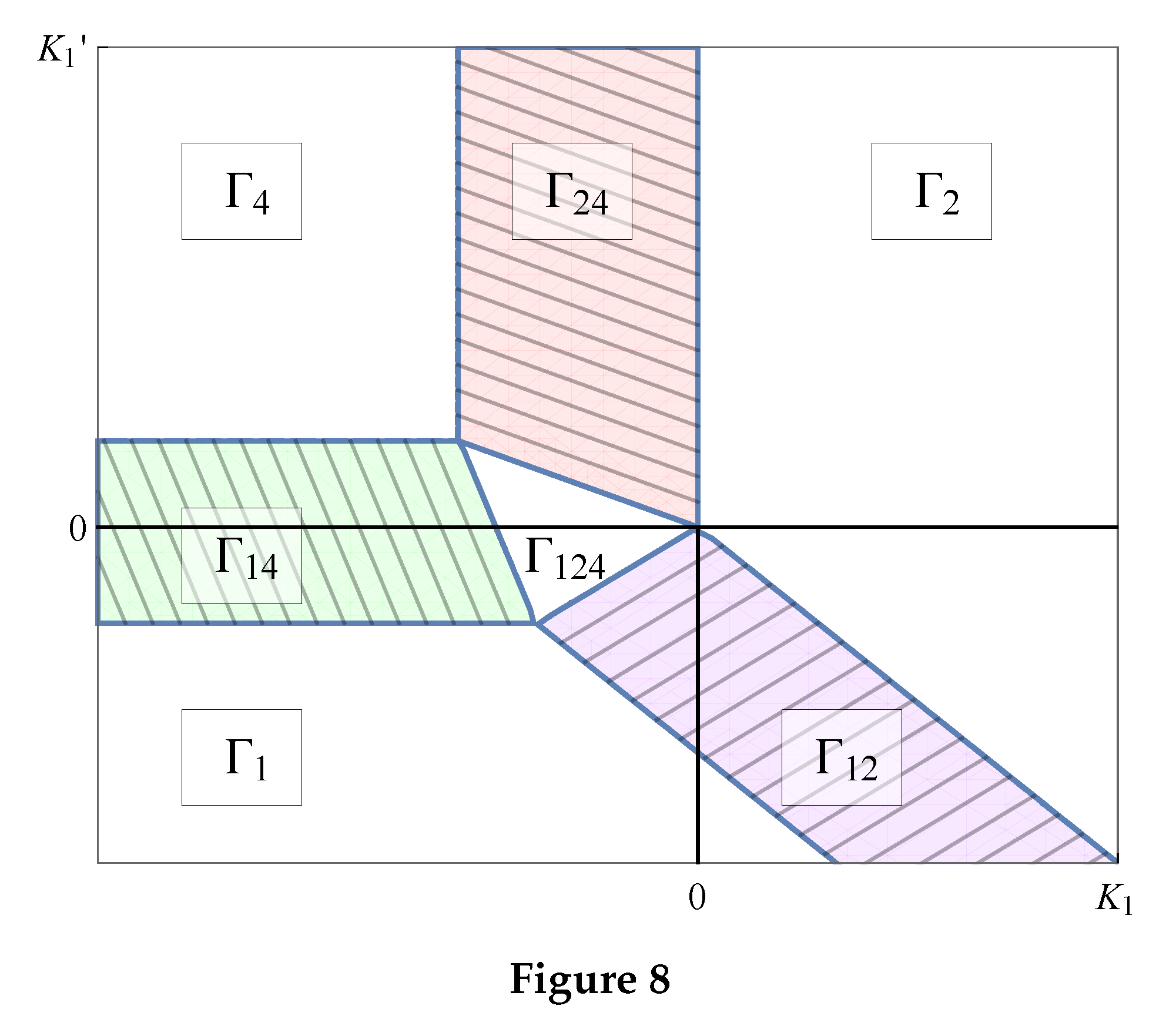
Figure shows the phase diagram of the system described by the TDP (88) in coordinates $\alpha =H_A/H_E$, ${\alpha }_H=H/H_E$. It can be seen from the figure that at $\alpha \lesssim 1$, i.e. at $H_A\lesssim H_E$, there is always the phase with flipped sublattices FL (between the phase lines 1 and 3). The transition from the antiferromagnetic phases (AFM) to the FL-phase can be delayed, this phenomenon analogous to overheating during a first-order phase transition such as melting. The reverse transition FL–AFM can also be delayed (this is shown in Figure by the lines 2 and 4). At $\alpha >1$, the FL-phase is absent. With an increase in the external field at $\alpha \ge 1$, the AFM-phase transforms into the FM-phase, i.e. into a ferromagnet induced by the field. The region $\alpha >1$ of the phase diagram is the region of the metamagnetic state existence.

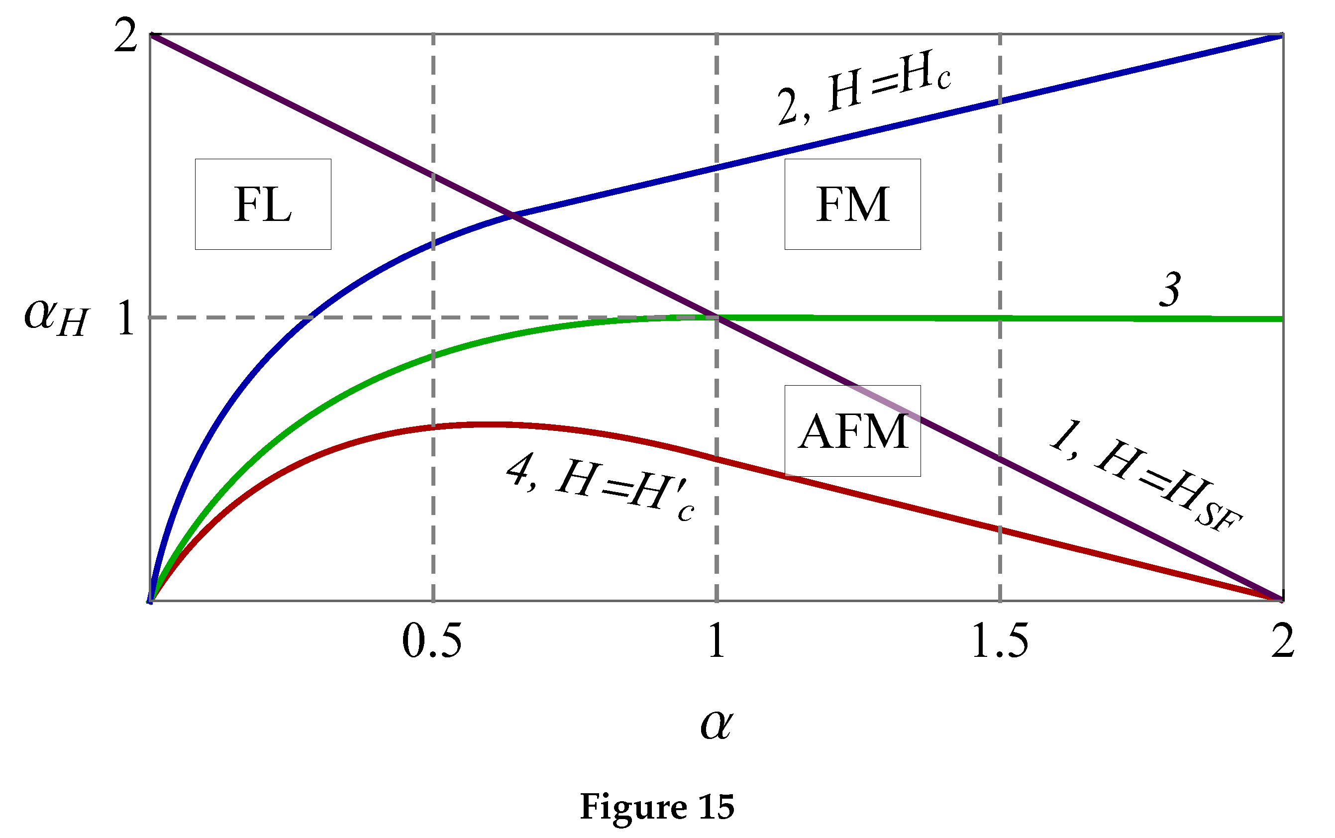
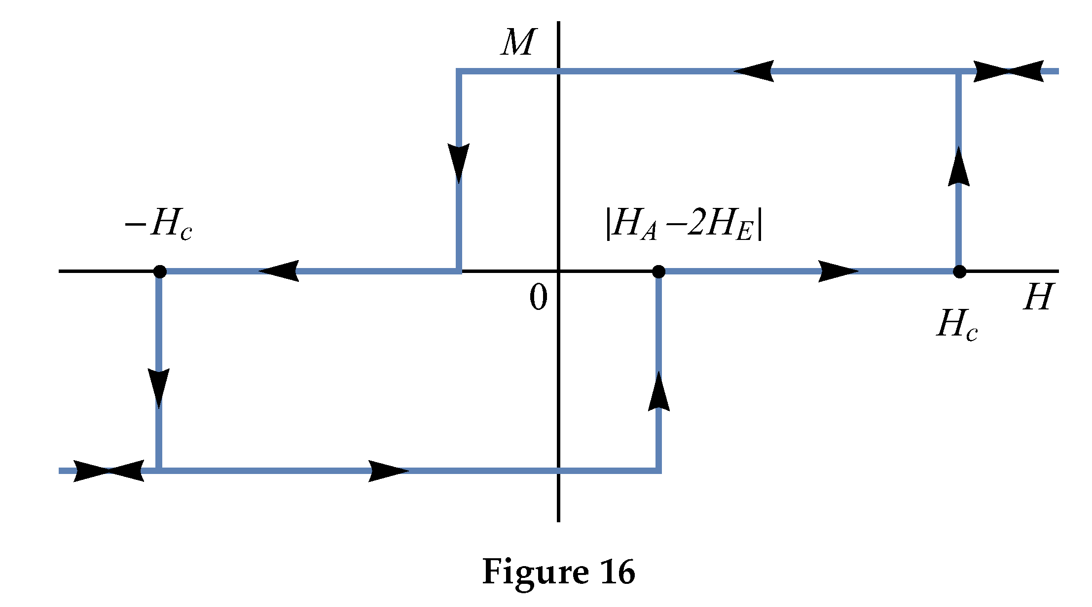
The transition AFM–FM in an external field is called the “spin-flip” transition. A typical magnetization curve for metamagnets is shown in Figure . We note that a decrease in the field to zero after the spin-flip transition can not be accompanied by a return of the system to the AFM state (this requires $H_A>2H_E$). Thus, after turning off the field, the metamagnet can remain in the FM state, it will have remanent magnetization. If the value of $|H_A-2H_E|$, which plays the role of the coercive force in this case, is sufficiently large, then such a metamagnet can be used as the material for permanent magnets.

4. Elastic and Magnetoelastic Properties of Rhombic Magnets at SR Transitions

4.1. Magnetostriction at SR Transitions

Consider a rhombic magnet with a SR transition in one of the crystallographic planes (e.g. $ac$-plane). Along with ${\Phi }_{\mathrm{an}}$ from (28), the TDP of the crystal will include the elastic and magnetoelastic energies:

$$\begin{array}{cc}\hfill {\Phi }_{\mathrm{el}}=& \frac{1}{2}{c}_{11}{\epsilon }_{xx}^2+\frac{1}{2}{c}_{22}{\epsilon }_{yy}^2+\frac{1}{2}{c}_{33}{\epsilon }_{zz}^2+c_{12}{\epsilon }_{xx}{\epsilon }_{yy}+\hfill \\ \hfill & c_{13}{\epsilon }_{xx}{\epsilon }_{zz}+c_{23}{\epsilon }_{yy}{\epsilon }_{zz}+2c_{44}{\epsilon }_{yz}^2+2c_{55}{\epsilon }_{xz}^2+2c_{66}{\epsilon }_{xy}^2,\hfill \end{array}$$

(92)

$$\begin{array}{cc}\hfill {\Phi }_{\mathrm{m}-\mathrm{el}}=& \left(L_a{\epsilon }_{xx}+L_b{\epsilon }_{yy}+L_c{\epsilon }_{zz}\right){sin}^2\theta +\frac{1}{2}{\mu }_2{\epsilon }_{xz}sin2\theta ;\hfill \end{array}$$

(93)

moreover, the form of ${\Phi }_{\mathrm{m}-\mathrm{el}}$ is determined by choosing the SR in the $ac$-plane.

Minimizing the TDP by deformations ${\epsilon }_{ij}$ in the absence of external mechanical stresses, we obtain:

$${\epsilon }_{ii}=-{\displaystyle \frac{L_i}{c_{ii}}}{sin}^2\theta ,{\epsilon }_{xz}=-{\displaystyle \frac{{\mu }_2}{8c_{55}}}sin2\theta ,{\epsilon }_{yz}={\epsilon }_{xy}=0.$$

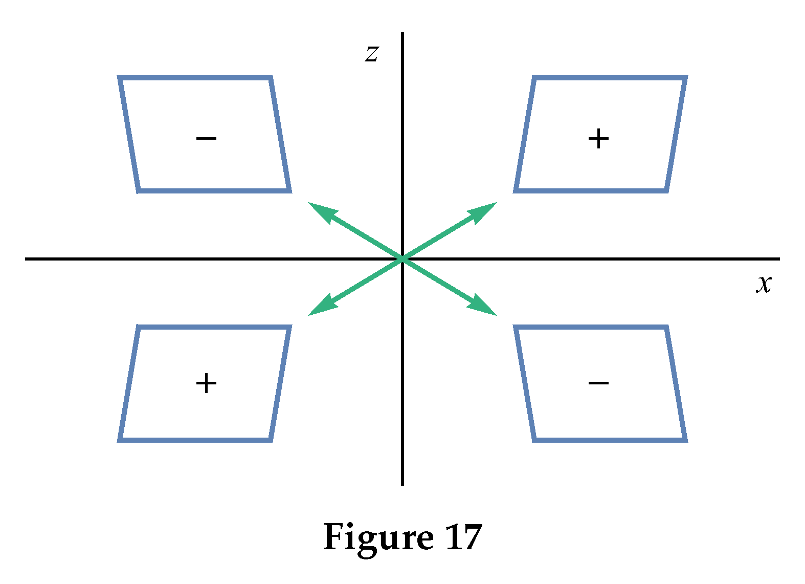
In this way, at a smooth SR transition $M_z\to M_x$, along with the usual magnetostrictive deformations ${\epsilon }_{xx,yy,zz}$ that do not change the rhombic symmetry of the crystal, shear (monoclinic) deformations appear in the plane of magnetic moments rotation, reaching a maximum at $\theta =\pm {45}^{\circ }$, $\pm {135}^{\circ }$. The ordinary deformations ${\epsilon }_{ii}$ are even, and the monoclinic deformation ${\epsilon }_{xz}$ is the odd function of the order parameter $\theta$. Therefore, if the magnetostrictive deformations are insensitive to the domain structure, then the monoclinic deformation differs in sign in domains with different signs of the order parameter (Figure ).

During the SR transition $M_z\to M_x$ induced by an external magnetic field $\overrightarrow{H}\left|\right|x$, the nature of the magnetostrictive deformations in the rhombic ferromagnet will have the form shown schematically in Figure 8.

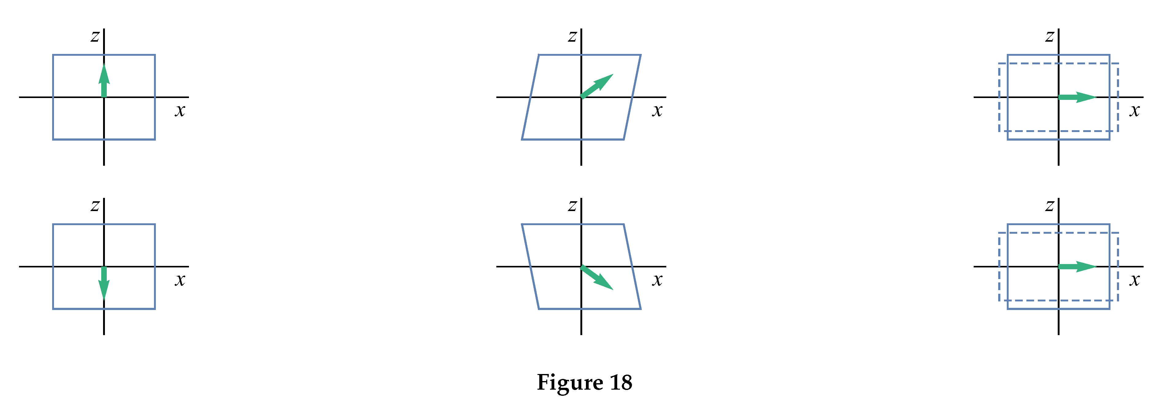
It is clear that the sample remagnetization by domain boundary offsets in the angular phase $M_{zx}$, for which small external magnetic fields are sufficient, will be accompanied by a change in the sign of the monoclinic deformation.

4.2. OPT Induced by External Mechanical Stresses

Below we consider a rhombic magnet with magnetic anisotropy of the form

$${\Phi }_{\mathrm{an}}=K_1{sin}^2\theta +K_2{sin}^4\theta ,$$

(94)

where $\theta$ is the orientation angle of a magnetic moment (or antiferromagnetism) vector in one of the crystallographic planes (e.g. $ac$-plane).

The action of external mechanical stresses (pressure) leads to elastic deformations of the sample. Under uniaxial compression along the c-axis, the components of the elastic deformation tensor in the rhombic crystal is determined according to

$${\epsilon }_{ij}=-p{S}_{ijzz}{\delta }_{ij},$$

(95)

where $S_{ijkl}$ is the elastic compliance tensor. Under bulk compression of the rhombic crystal, we have

$${\epsilon }_{ii}=-p\sum _j{S}_{iijj}.$$

(96)

If pressure is applied in the $ac$-plane at an angle of $\alpha$ to the a or c-axis, then it also causes the appearance of shear deformations. At $\alpha ={45}^{\circ }$

$${\epsilon }_{ii}=-\frac{1}{2}p\left(S_{ii33}+S_{ii11}\right),{\epsilon }_{ac}=\frac{1}{2}p{S}_{1313}.$$

(97)

When analyzing the OPT in the $ac$-plane, we represent the magnetoelastic energy in the form (92). It is clear that bulk compression, or compression along the crystallographic axes a, b, c of the rhombic crystal does not change the lattice symmetry and, due to the magnetoelastic coupling (92), it leads only to the change in the anisotropy constant $K_1$:

$$\Delta K_1=L_a{\epsilon }_{aa}+L_b{\epsilon }_{bb}+L_c{\epsilon }_{cc}=\left\{\begin{array}{c}-p\sum _j{L}_i{S}_{ii33}(c-\mathrm{axis}\mathrm{compression}),\hfill \\ -p\sum _{ij}{L}_i{S}_{iijj}(\mathrm{bulk}\mathrm{compression}).\hfill \end{array}\right.$$

(98)

If we assume that $K_2$, $L_{a,b,c}$ do not depend on temperature and $K_1$ depends linearly on T according to the relation (36), then the effect of pressure in this case will be reduced only to the shift in the beginning and end of the SR without changing the SR interval:

$${\displaystyle \frac{\partial T_1}{\partial p}}={\displaystyle \frac{\partial T_2}{\partial p}}=-{\displaystyle \frac{(T_2-T_1)}{2K_2}}{\displaystyle \frac{\partial K_1}{\partial p}},{\displaystyle \frac{\partial (T_2-T_1)}{\partial p}}=0.$$

(99)

For the values of the parameters that are characteristic of a number of orthoferrites RFeO$3$: $(T_2-T_1)\sim 10$ K, $K_2\sim 5·{10}^4$ erg · cm$-3$, ${\displaystyle \frac{\partial K_1}{\partial p}}\sim {10}^5$ erg · cm$-3·$ kbar$-1$, we have:

$${\displaystyle \frac{\partial T_{1,2}}{\partial p}}\sim 10{\displaystyle \frac{\mathrm{K}}{\mathrm{kbar}}}.$$

(100)

The presence of the shear component of mechanical stresses leads to a change in the rhombic symmetry of the crystal and an OPT induction in the $ac$-plane even at an arbitrarily small value of ${\epsilon }_{ac}$. The equilibrium value of the angle $\theta$ is determined in this case by the equation

$$tan2\theta =-{\displaystyle \frac{{\mu }_2{\epsilon }_{ac}}{K_1+\Delta K_1+2K_2{sin}^2\theta }}$$

(101)

at $cos2\theta \ne 0$. For the “magnetoelastic” susceptibility, we have

$${\left.{\displaystyle \frac{\partial \theta }{\partial {\epsilon }_{ac}}}\right|}_0=\left\{2.5\begin{array}{c}-{\displaystyle \frac{{\mu }_2}{2K_1}},\theta =0;\hfill \\ -{\displaystyle \frac{{\mu }_2}{2(K_1+2K_2)}},\theta ={\displaystyle \frac{\pi }{2}};\hfill \\ -{\displaystyle \frac{{\mu }_{2}cos2\theta }{2K_2{sin}^{2}2\theta }},0<\theta <{\displaystyle \frac{\pi }{2}}\hfill \end{array}\right.$$

(102)

(where the equation $\partial \Phi /\partial \theta =0$ is used). Thus, the magnetoelastic susceptibility ${\left.{\displaystyle \frac{\partial \theta }{\partial {\epsilon }_{ac}}}\right|}_0$ has a singularity at the points $T_1$ and $T_2$, i.e. the beginning and end of the smooth SR transition $\theta =0\to \theta =\pi /2$ (Figure ).

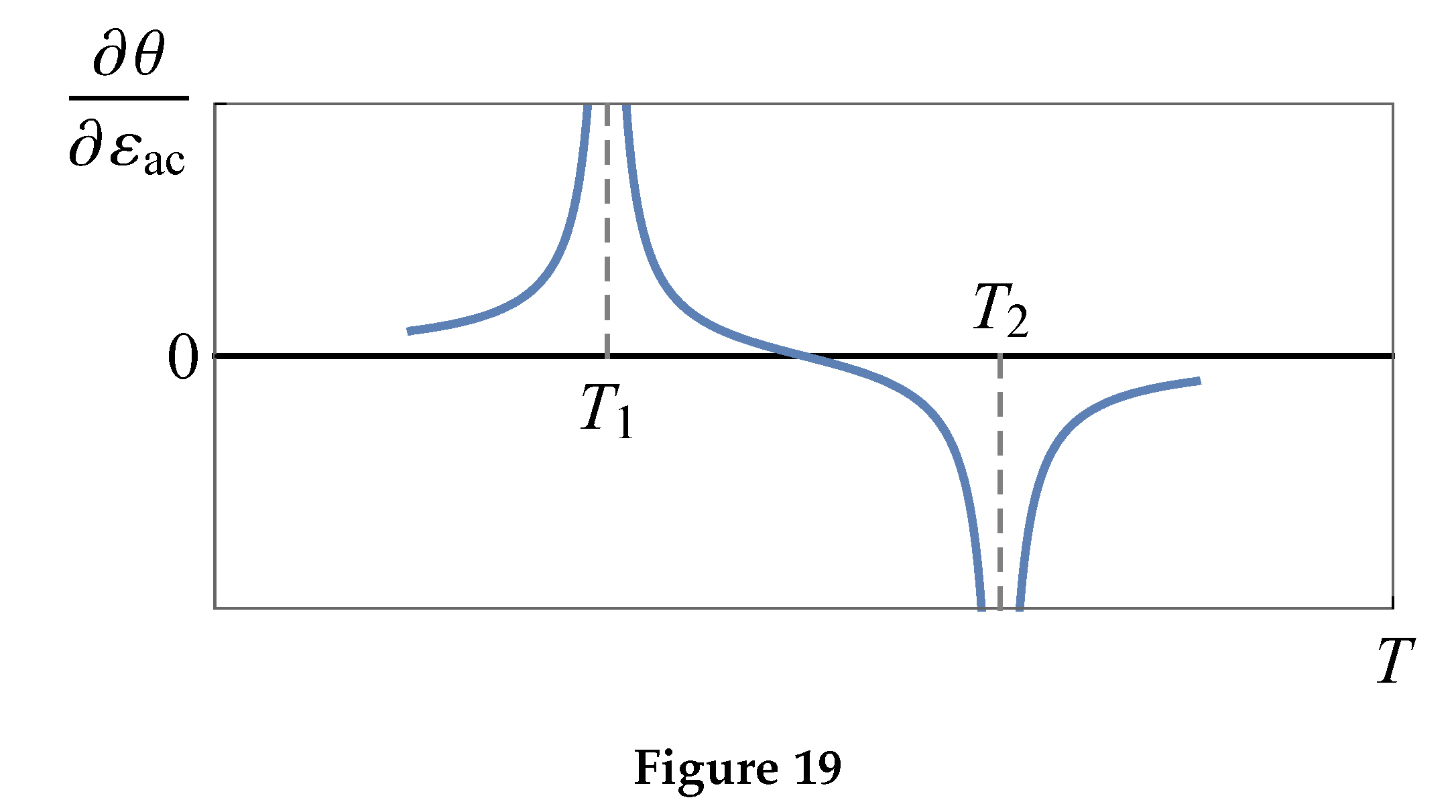
At a linear dependency of $K_1\left(T\right)$ this singularity is a characteristic of the Landau theory. Close to $T_1$ or $T_2$, we have ${\left.{\displaystyle \frac{\partial \theta }{\partial {\epsilon }_{ac}}}\right|}_0\sim {(T-T_{1,2})}^{-1}$.

Note that for large shear deformations ${\epsilon }_{ac}$ and small values of $K_{1.2}$, the equilibrium value of angle $\theta$ will approach $\pm \pi /2$. The sign of $\theta$ will then be determined by the signs of $\mu$ and ${\epsilon }_{ac}$.

4.3. Behavior of Elastic Modules at SR Transitions

The components of an elastic compliance tensor $S_{\mu \nu }$ play a role of elastic susceptibilities and have singularities in SR transition regions.

For a rhombic crystal with the spontaneous SR transition in the $ac$-plane, the elastic modules $S_{11,22,23}$ and $S_{12,13,23}$ will change sharply at the PT points $M_z\to M_{zx}$ and $M_{zx}\to M_x$, since the associated with ${\epsilon }_{ii}$ and mechanical stresses ${\sigma }_{ii}$ term in ${\Phi }_{\mathrm{m}-\mathrm{el}}$ is quadratic in the order parameter $\theta$ or ${\theta }^{\prime }=\pi /2-\theta$. The elastic modulus $S_{55}$ will have a hyperbolic type divergence at these points, since the associated with ${\epsilon }_{ac}$ and ${\sigma }_{ac}$ (${\epsilon }_{ac}=S_{55}{\sigma }_{ac}$) term in ${\Phi }_{\mathrm{m}-\mathrm{el}}$ is linear in the order parameter. The modules $S_{44}$, $S_{66}$ do not have singularities in the SR transition region of the $ac$-plane.

Of practical interest is an analysis of the behavior of constants $C_{\mu \nu }$ (inverse elastic susceptibilities) during the SR transitions, which are easily determined experimentally in terms of sound propagation velocities. For example, for $C_{55}$ at the SR transition $M_z\to M_x$ in the $ac$-plane, we have (Figure )

$$C_{55}=C_{55}^{\left(0\right)}+\left\{2.5\begin{array}{c}-{\displaystyle \frac{{\mu }_2^2}{4K_1}},M_z-\mathrm{phase};\hfill \\ +{\displaystyle \frac{{\mu }_2^2}{8K_1}},M_{xz}-\mathrm{phase},\theta \ge 0;\hfill \\ -{\displaystyle \frac{{\mu }_2^2}{8(K_1+2K_2)}},M_{xz}-\mathrm{phase},\theta \le {\displaystyle \frac{\pi }{2}};\hfill \\ +{\displaystyle \frac{{\mu }_2^2}{4(K_1+2K_2)}},M_x-\mathrm{phase}.\hfill \end{array}\right.$$

(103)

A sharp decrease in the shear elastic constant $C_{55}$ at the points $T_1$ and $T_2$ of the SR transitions $M_{zx}\to M_x$ and $M_z\to M_{zx}$ leads to a corresponding sharp drop in the transverse sound velocity

$$v_{xz}^T=\sqrt{C_{55}/p}$$

(104)

and an anomalous “softening” of the lattice with respect to shear mechanical stresses in the plane of a magnetic moments rotation.

References

- Belov, K.P.; Zvezdin, A.K.; Kadomtseva, A.M.; Levitin, R.Z. Orientational Transitions in Rare-Earth Magnets; Nauka: Moscow, 1979. [Google Scholar]
- Vonsovsky, S.V. Magnetism; Nauka: Moscow, 1971. [Google Scholar]
- Turov, E.A. Physical Properties of Magnetically Ordered Crystals; Publishing House of the Academy of Sciences of the USSR: Moscow, 1963. [Google Scholar]
- Moskvin, A. Structure–Property Relationships for Weak Ferromagnetic Perovskites. Magnetochemistry 2021, 7, 111. [Google Scholar] [CrossRef]
- Moskvin, A. S. JETP 2021, 132((4)), 517–547. [CrossRef]
- Moskvin, A.S. Dzyaloshinskii–Moriya Coupling in 3d Insulators. Condens. Matter 2019, 4, 84. [Google Scholar] [CrossRef]
- Moskvin, A. S. JMMM 2018, 463, 50. [CrossRef]
- Moskvin, A. S. JMMM 2016, 400, 117. [CrossRef]
- Moskvin, A.; Vasinovich, E.; Shadrin, A. Simple Realistic Model of Spin Reorientation in 4f-3d Compounds. Magnetochemistry 2022, 8, 45. [Google Scholar] [CrossRef]
- Vasinovich, E.V.; Moskvin, A.S. Physics of the Solid State 2024, Vol. 66(No. 6).
Disclaimer/Publisher’s Note: The statements, opinions and data contained in all publications are solely those of the individual author(s) and contributor(s) and not of MDPI and/or the editor(s). MDPI and/or the editor(s) disclaim responsibility for any injury to people or property resulting from any ideas, methods, instructions or products referred to in the content. |
© 2025 by the authors. Licensee MDPI, Basel, Switzerland. This article is an open access article distributed under the terms and conditions of the Creative Commons Attribution (CC BY) license (http://creativecommons.org/licenses/by/4.0/).
Copyright: This open access article is published under a Creative Commons CC BY 4.0 license, which permit the free download, distribution, and reuse, provided that the author and preprint are cited in any reuse.