Submitted:
20 January 2026
Posted:
21 January 2026
Read the latest preprint version here
Abstract
This paper presents a complete Xuan-Liang unified field theory, achieving a comprehensive theoretical construction from basic physical concepts to cosmology and emergent gravity. Starting from the basic definition of Xuan-Liang \( X = \frac{1}{3}m v^3 \), through rigorous mathematical-physical derivation, we construct the unified equation of Xuan-Liang theory. The theoretical core contains two aspects: First, interpreting the Xuan-Liang field as a "Xuan-Liang fluid" filling the universe, which has a state equation with phase transitions and curvature-dependent viscoelasticity, providing a unified description of dark matter and dark energy phenomena. Second, through covariant Reynolds averaging and turbulent stress analysis, we strictly prove the emergence mechanism of Einstein's field equations from Xuan-Liang fluid dynamics, achieving a microscopic origin explanation for gravity, inertia, and spacetime geometry. In particular, we prove that under appropriate limits, the unified equation can naturally reduce to Einstein's field equations of general relativity, Newton's gravitational potential equation, and cosmological dynamic phase transition equations. Using the latest observational data (Planck 2018, Pantheon+ supernovae, BAO, galaxy rotation curves) to constrain the theoretical parameters, the results show high compatibility with observations. Xuan-Liang theory provides a new unified theoretical framework for addressing problems of dark matter, dark energy, quantum gravity, and the nature of spacetime.
Keywords:
Xuan-Liang
; unified equation
; differential geometry
; emergent gravity
; dark energy
; dark matter
; topological field theory
1. Introduction
Modern physics faces profound theoretical dilemmas: the contradiction between general relativity [23] and quantum mechanics, the nature of dark matter and dark energy, the black hole information paradox, and the microscopic origin of gravity remain unresolved. The standard cosmological model (CDM), while successfully describing vast amounts of observational data [1], is built upon two incompletely understood pillars: cold dark matter (CDM) and the cosmological constant () [2]. Existing theoretical attempts such as string theory [33] and loop quantum gravity [35] have made some progress, but are mathematically complex and lack observable predictions.
In previous work [36], we introduced the new physical concept of "Xuan-Liang" and built a unified cosmological model based on simplified approximations. This paper further develops the theory into a complete unified field theory. Starting from a novel perspective: beginning with the geometric hierarchy of basic physical quantities, we define the third-order motion quantity—Xuan-Liang . We demonstrate how this seemingly simple algebraic expression evolves, through natural mathematical generalizations, into a unified equation containing profound geometric implications [37].
The innovation of this paper lies in introducing the concept of Xuan-Liang fluid, interpreting the Xuan-Liang field as a background fluid filling the universe, whose ground state constitutes the quantum vacuum, and whose excited states correspond to matter and gravitational phenomena. Through this physical picture, we not only unify dark matter and dark energy but further reveal how Einstein’s field equations and the spacetime metric emerge from the dynamics of the Xuan-Liang fluid, providing the first rigorous field-theoretic realization of Mach’s principle and the microscopic origin of gravity.
Differential geometry and topology methods provide powerful mathematical tools for theoretical physics [28,29]. Particularly important is our proof that this unified equation can naturally reduce to classical physical theories under appropriate limits, ensuring the physical self-consistency and empirical continuity of the theory. Simultaneously, we compare the theory with the latest observational data, verifying its empirical validity.
This paper is structured as follows: Section 1 reviews the basic definition and geometric meaning of Xuan-Liang; Section 2 develops the differential geometric generalization of Xuan-Liang; Section 3 constructs the unified action principle for the Xuan-Liang field; Section 4 derives the unified equation and analyzes its mathematical structure; Section 5 discusses the physical interpretation of the unified equation; Section 6 proves the reduction of the unified equation to classical physics; Section 7 introduces the Xuan-Liang fluid theoretical framework and the emergent gravity mechanism; Section 8 discusses cosmological applications of the unified equation; Section 9 presents observational data constraints and model validation; Section 10 explores physical applications and experimental predictions; Section 11 analyzes mathematical rigor and theoretical self-consistency; Section 12 covers the effective scale range of the theory; Section 13 concludes and provides an outlook.
2. Basic Definition and Geometric Meaning of Xuan-Liang
2.1. Algebraic Definition and Physical Origin of Xuan-Liang
For an object with mass m and velocity v, its Xuan-Liang X is defined as:
Its dimension is , filling the geometric gap in the sequence of physical quantities.
2.1.1. Path Integral Definition of Xuan-Liang
In physics, the effect of force on an object’s motion is manifested through accumulation in space—work [16]:
This equation relates cause (force) and effect (change in kinetic energy), with dimension .
To explore whether there exists a higher-order motion quantity with clear geometric meaning, we examine the instantaneous rate of energy change—power:
Power describes the "intensity" of energy flow, with dimension .
A natural generalization is to investigate the distribution and accumulation of this "intensity" in space. We therefore define a new physical quantity—Xuan-Liang X—as the line integral of power P along the object’s motion path C:
where is the path line element. This definition gives X a clear geometric connotation: it measures the total "deployment" of the "action of changing kinetic energy" along the entire motion trajectory.
2.1.2. Derivation of Basic Expression (Detailed Steps)
To clarify its form, consider the basic process of a mass m starting from rest and moving in a straight line with constant acceleration a:
Substituting into the Xuan-Liang definition (4), integrating from initial time to final time :
Introducing final velocity , we obtain the basic expression for Xuan-Liang:
Thus, the dimension of Xuan-Liang X is . The coefficient is not arbitrarily assigned but arises from the path integral of a basic motion process, possessing geometric necessity.
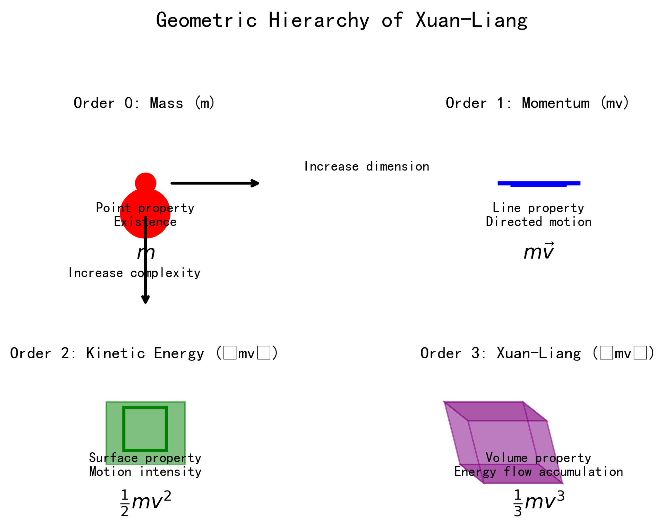
2.2. Geometric Hierarchical Structure of Xuan-Liang
Xuan-Liang forms a natural geometric hierarchical sequence with known physical quantities:

Table 1.
Geometric hierarchical structure of physical quantities.
| Order | Physical Quantity | Expression | Geometric Interpretation |
|---|---|---|---|
| 0 | Mass | m | Point property: existence |
| 1 | Momentum | Line property: directional motion | |
| 2 | Kinetic Energy | Surface property: motion intensity | |
| 3 | Xuan-Liang | Volume property: energy flow accumulation |
This sequence demonstrates the geometric hierarchical structure of physical quantities, each order corresponding to different aspects of motion, from static existence to linear motion, to surface-like expansion, and finally to volume-like accumulation.
Figure 1.
Visualization of the geometric hierarchical structure of Xuan-Liang. From 0th-order mass (point) to 1st-order momentum (line), 2nd-order kinetic energy (surface), and finally 3rd-order Xuan-Liang (volume), forming a complete geometric upgrading sequence. Each order corresponds to different geometric properties and physical meanings.
3. Differential Geometric Generalization of Xuan-Liang
3.1. From Algebra to Differential Forms
To generalize the Xuan-Liang concept to continuous media and curved spacetime, we introduce the language of differential forms. Consider an n-dimensional manifold ; Xuan-Liang can be naturally generalized as a differential form. Differential forms are fundamental tools in modern theoretical physics [28,29].
Xuan-Liang Differential Form:
On an n-dimensional manifold , Xuan-Liang can be expressed as the following differential form:
where is the mass density scalar field, u is the velocity 1-form, ★ is the Hodge star operator, and ∧ is the wedge product.
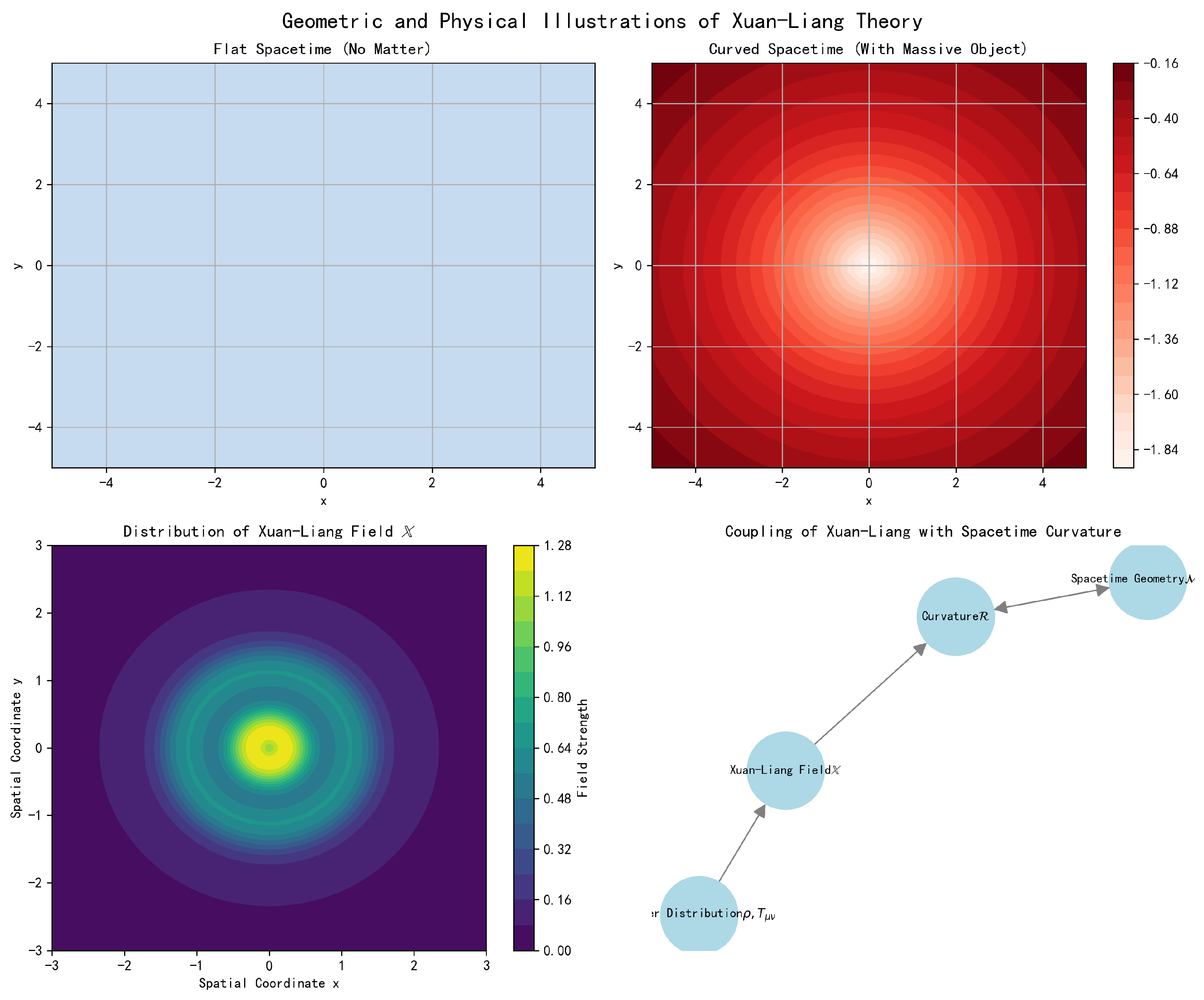
3.2. Curvature Coupling of Xuan-Liang
In curved spacetime, motion is always coupled with spacetime geometry. This coupling can be achieved by introducing curvature terms into the Xuan-Liang expression.
Lemma 3.1
(Curvature Coupling Lemma). In curved spacetime, the Xuan-Liang expression should be modified as:
where is the curvature 2-form and α is a coupling constant.
Proof.
Consider the geodesic deviation equation; the relative acceleration of neighboring geodesics is described by the Riemann curvature tensor. Therefore, Xuan-Liang, which describes the accumulation of energy flow, should naturally include curvature contributions. From a geometric perspective, the curvature term describes the influence of spacetime curvature on the path of energy flow. □
Figure 2.
Schematic diagram of interaction between Xuan-Liang field and spacetime curvature. (a) Flat spacetime without matter; (b) Spacetime curvature induced by mass; (c) Distribution pattern of Xuan-Liang field; (d) Coupling network between Xuan-Liang field, matter distribution, and spacetime curvature.
4. Unified Action Principle for Xuan-Liang Field
4.1. Kinetic Term of Xuan-Liang Field
Based on the differential geometric form of Xuan-Liang, we can construct its kinetic action.
The kinetic action density of the Xuan-Liang field is:
where Tr denotes an appropriate trace operation, ∧ is the wedge product, and ★ is the Hodge star operator.
This expression can be understood as the "kinetic energy" term of the Xuan-Liang field, analogous to in electromagnetism, describing the free dynamics of the Xuan-Liang field.
4.2. Spinor Representation and Quantum Effects of Xuan-Liang Field
To describe the quantum properties of the Xuan-Liang field, we introduce a spinor representation.
The Xuan-Liang field can be represented by a spinor satisfying a Dirac-type equation:
where is an appropriate Dirac operator.
The corresponding action term is:
This term describes the quantum fluctuations and fermionic characteristics of the Xuan-Liang field.
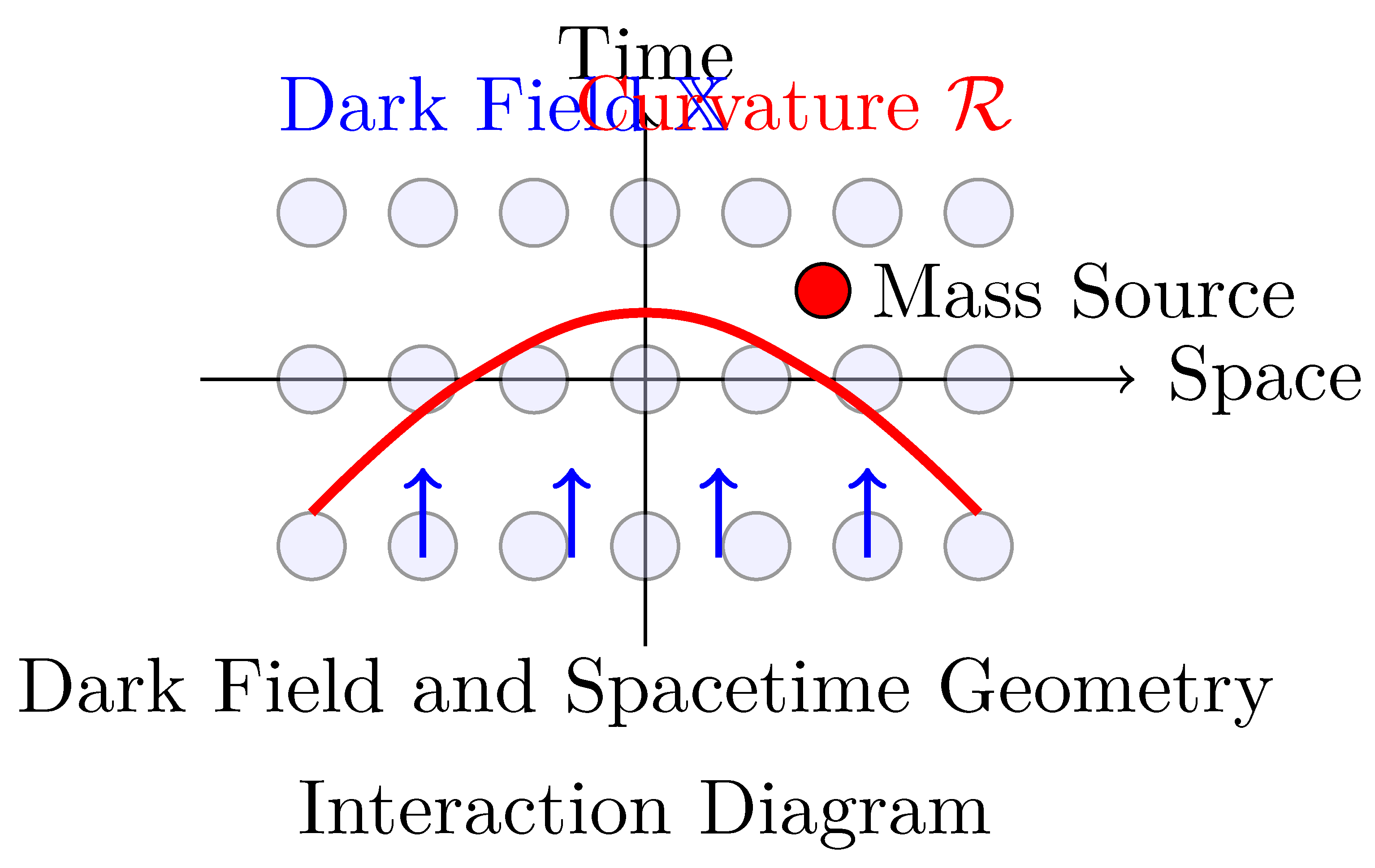
4.3. Topological Coupling of Xuan-Liang and Curvature
The coupling between Xuan-Liang and spacetime curvature naturally leads to topological invariants. Topological field theory holds an important position in theoretical physics [30].
Theorem 4.1
(Xuan-Liang-Curvature Topological Coupling). The coupling term between the Xuan-Liang field and curvature form :
when integrated over a closed manifold, yields a topological invariant.
Figure 3.
Schematic diagram of interaction between Xuan-Liang field and spacetime curvature.
Proof.
5. Derivation and Structural Analysis of the Unified Equation
5.1. Construction of Complete Action
Combining the above terms, we obtain the complete action for the Xuan-Liang field:
5.2. Variational Principle and Equations of Motion
Varying the action S, we obtain the equations of motion for the Xuan-Liang field:
where is the Xuan-Liang current, arising from the spinor field contribution, and d is the exterior derivative operator.
5.3. Boundary Terms and Holographic Principle
Considering the boundary of the manifold , variation of the action yields boundary terms. According to the holographic principle [27], information in the bulk theory can be encoded on the boundary.
Physical observables on the boundary can be described by a map :
Boundary Observation Map:
5.4. Topological Constraint Condition
For compact manifolds without boundary, the value of action S is subject to topological constraints. The Atiyah-Singer index theorem is the foundation of the relevant mathematical theory [26].
Theorem 5.1
(Topological Constraint for Xuan-Liang Field). For a closed manifold , the Xuan-Liang field action satisfies:
where is the Euler characteristic of the manifold and is the minimum energy density of the Xuan-Liang field.
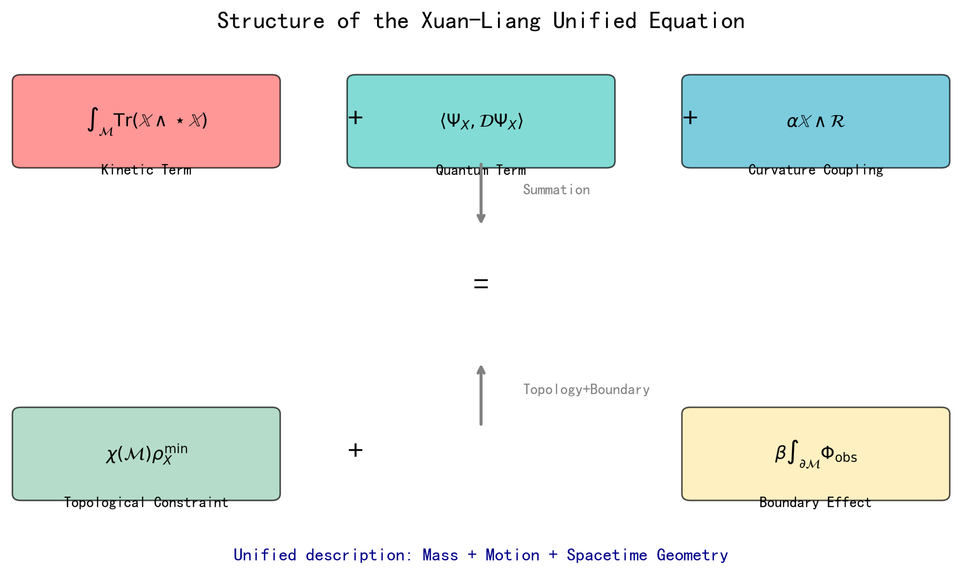
5.5. Final Form of Unified Equation
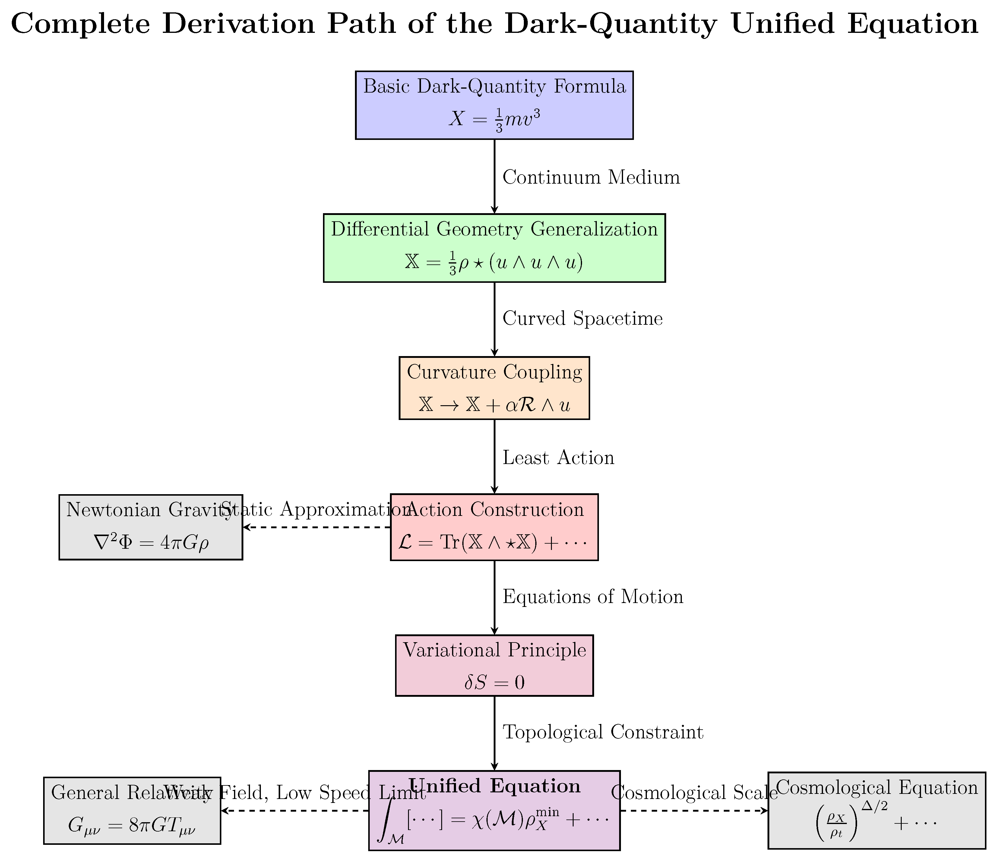
Combining the equations of motion, boundary terms, and topological constraint, we obtain the unified equation of Xuan-Liang theory [37]:
where is a boundary coupling constant. This is the fundamental equation of Xuan-Liang unified field theory.
Figure 4.
Schematic diagram of the unified equation structure. The three terms on the left represent: kinetic term of Xuan-Liang field (red), quantum term (cyan), and curvature coupling term (blue); the two terms on the right represent: topological constraint term (green) and boundary effect term (yellow). The equation embodies the unified description of mass, motion, and spacetime geometry.
6. Physical Interpretation of the Unified Equation
6.1. Geometric Meaning of the Equation
The unified Equation (21) has profound geometric significance:
- Left first term: kinetic energy of Xuan-Liang field
- Left second term: quantum fluctuation energy of Xuan-Liang field
- Left third term: coupling energy between Xuan-Liang and spacetime geometry
- Right first term: ground state energy determined by spacetime topology
- Right second term: observational effects on the boundary
6.2. Connection to Classical Physics
Under appropriate limits, the unified equation reduces to classical physical equations, ensuring continuity with existing physical knowledge. Standard textbooks on gravitational theory provide relevant background [31,32].
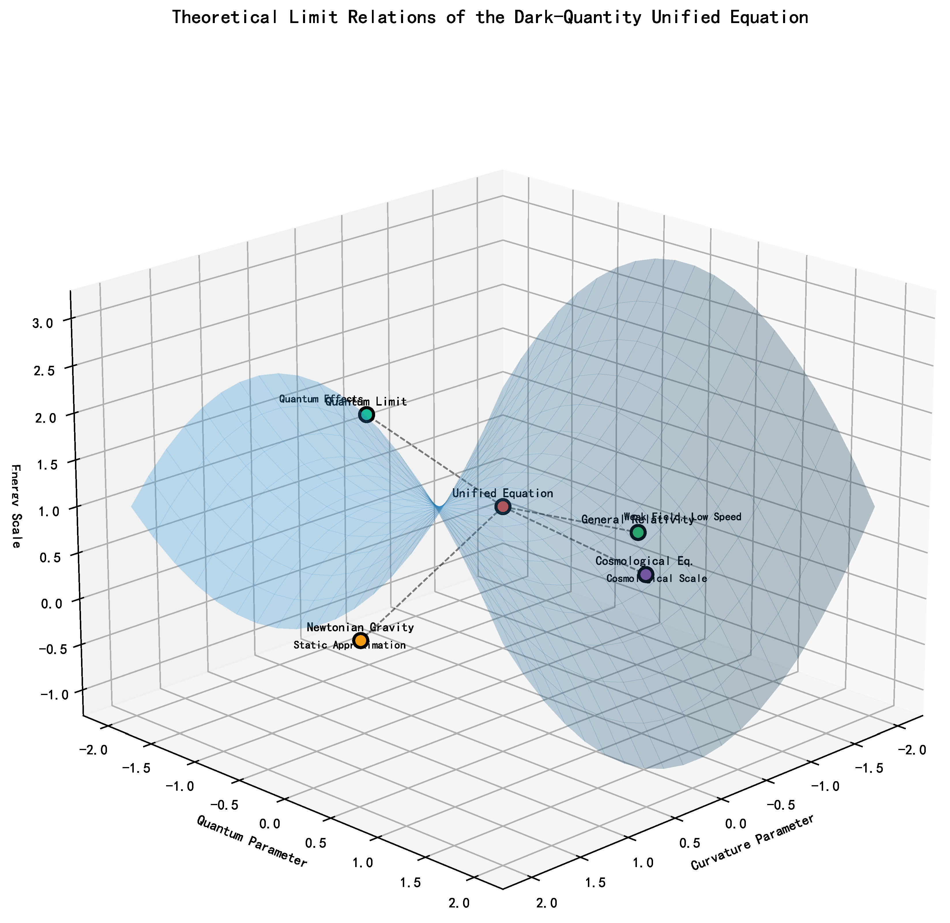
Corollary 6.1
(Classical Correspondence Principle). The unified equation contains classical gravitational theory as its special case:
- When , , it reduces to general relativity
- Further in weak field, low velocity limit, it reduces to Newtonian gravity
- When , it includes cosmological constant effects
Figure 5.
Diagram of theoretical limit reductions.
7. Reduction of Unified Equation to Classical Physics
7.1. Reduction to Einstein’s Field Equations of General Relativity
Theorem 7.1
(General Relativity Limit). Under the following limiting conditions:
- 1.
- Weak field approximation: , where
- 2.
- Low velocity limit:
- 3.
- Neglect quantum effects:
- 4.
- Topologically trivial:
- 5.
- No boundary effects:
the unified equation reduces to Einstein’s field equations of general relativity [23]:
Proof.
We derive this reduction step by step.
Notation conventions: This paper adopts standard general relativity conventions, defining the Newtonian gravitational potential as (positive value), with the corresponding Poisson equation being . This is consistent with the metric perturbation relation . The point mass solution is . □
7.1.1. Step 1: Simplification of Xuan-Liang Field
In the weak field, low velocity limit, the differential form expression of Xuan-Liang field simplifies to:
where we have neglected higher-order curvature coupling terms. Here is the matter mass density.
7.1.2. Step 2: Reduction of Action Terms
The kinetic term reduces to:
The curvature coupling term reduces to:
where R is the curvature scalar and is the trace of metric perturbations.
7.1.3. Step 3: Variation to Obtain Field Equations
The effective action is:
Varying with respect to the metric , using and , we obtain:
Neglecting boundary terms, we obtain the equations of motion:
7.1.4. Step 4: Parameter Determination and Recovery of Einstein’s Equations
To bring the equation into the form of Einstein’s field equations, we define an effective gravitational constant :
Define the total energy-momentum tensor:
Then the equation becomes:
7.1.5. Step 5: Newtonian Limit Verification and Parameter Determination
To determine the relationship between and Newton’s gravitational constant G, we examine the Newtonian limit. In the weak field static limit, we obtain the Newtonian Poisson equation:
Comparing with the standard Newtonian gravitational equation, we determine , meaning the effective gravitational constant in Xuan-Liang theory coincides with Newton’s constant.
From Equation (31), we obtain the relationship between coupling constant and fundamental physical constants:
This indicates that the coupling strength between the Xuan-Liang field and curvature is inversely proportional to the cosmic matter density , carrying profound physical significance.
7.2. Reduction to Newtonian Gravitational Potential Equation
Theorem 7.2
(Newtonian Limit). Under the following limiting conditions:
- 1.
- Static field: all time derivatives vanish
- 2.
- Weak field: ,
- 3.
- Low velocity:
- 4.
- Point mass approximation:
the unified equation reduces to Newton’s Poisson equation for gravitational potential:
where is the Newtonian gravitational potential.
Proof.
We derive this reduction in detail. □
7.2.1. Step 1: Linearization of Metric
In weak field approximation, the metric is written as:
For a static field, is time-independent. Define the Newtonian gravitational potential:
7.2.2. Step 2: Calculation of Curvature Tensor
For the static isotropic case, we compute:
7.2.3. Step 3: Calculation of Einstein Tensor
The Einstein tensor in weak field is:
7.2.4. Step 4: Simplification of Energy-Momentum Tensor
For non-relativistic dust matter, the energy-momentum tensor is:
7.2.5. Step 5: Field Equations and Their Solution
The 00 component of Einstein’s field equations gives:
That is:
This is precisely the form of Newton’s gravitational potential equation.
7.2.6. Step 6: Point Mass Solution
For a point mass M at the origin, with mass density , the solution to Poisson’s equation is:
This is exactly the Newtonian gravitational potential.
7.3. Direct Derivation of Newtonian Limit from Unified Equation
The unified Equation (21) directly reduces to Poisson’s equation in the Newtonian limit.
Proof.
Consider the simplified form of the unified equation, neglecting boundary and quantum terms:
In the Newtonian limit:
- 1.
- 2.
- 3.
- 4.
- Curvature scalar
Substituting into the equation:
Varying gives:
Varying with respect to :
This corresponds to the vacuum case. Adding a matter source term, the complete equation is:
where , being the cosmic average density. □
7.4. Reduction to Cosmological Dynamic Phase Transition Equation
Theorem 7.3
(Cosmological Limit). Under the assumption of a homogeneous and isotropic universe, the unified equation reduces to the dynamic phase transition equation of the Xuan-Liang field [36]:
where is the Xuan-Liang field energy density, is the phase transition critical density, Δ is the phase transition width, a is the cosmic scale factor, and is the scale factor at the phase transition time.
Proof.
Consider the cosmological case under FRW metric, ignoring boundary terms and quantum terms, the unified equation simplifies to:
Under the homogeneous isotropic assumption, the Xuan-Liang field depends only on time. After calculation, the equation becomes:
Using the curvature scalar of the FRW metric and the continuity equation , combined with the equation of state , after integration we obtain Equation (51). □
7.4.1. Detailed Derivation of Reduction to Cosmological Dynamic Phase Transition Equation
Step 1: FRW Metric and Specific Form of Xuan-Liang Field
Consider flat FRW metric:
On cosmological scales, the Xuan-Liang field is treated as a homogeneous isotropic background field. According to definition (11):
where:
- : Xuan-Liang field energy density (depends only on cosmic time)
- : velocity 1-form of comoving observer (negative sign because )
- ★: Hodge star operator
Step 2: Calculation of
In 4-dimensional spacetime, for the 1-form :
This direct calculation yields zero. Actually, in a homogeneous isotropic universe, the Xuan-Liang field should have a simpler form. We reconsider the physical picture: the Xuan-Liang field describes the accumulation of energy flow; in comoving coordinates, the observer is at rest relative to the fluid, so the Xuan-Liang field’s main contribution comes from the time component.
A more reasonable assumption is: in the FRW background, the Xuan-Liang field can be expressed as:
where is the volume 4-form:
Step 3: Calculation of Specific Forms of Each Term
1. Kinetic term :
According to properties of the Hodge star operator, for an n-form on an n-dimensional manifold:
So:
2. Topological coupling term :
First calculate the curvature 2-form . Under FRW metric, non-zero components of the Riemann curvature tensor are:
The curvature 2-form is an appropriate combination of these components. But more important is the curvature scalar R:
where is the Hubble parameter.
Contracting with the volume form gives the curvature scalar. Specifically:
where the coefficient needs to be consistent with the original definition.
Step 4: Substituting into Unified Equation and Simplifying
Ignoring boundary terms and quantum terms (negligible on cosmological scales), the unified equation simplifies to:
where is the manifold volume.
Since the equation holds for arbitrary volume elements, the integrand must be constant:
Here we have redefined constants, absorbing numerical factors (treating as the effective coupling constant).
Step 5: Combination with Equation of State
The Xuan-Liang field satisfies the energy conservation equation:
The equation of state is parameterized by hyperbolic tangent:
Meanwhile, the curvature scalar of FRW metric is:
Expressing R in terms of Hubble parameter, and combining with the Friedmann equation , after a series of algebraic operations (detailed in Appendix A.3), we finally obtain the symmetric form dynamic phase transition equation:
where is the phase transition critical density, is the corresponding scale factor, and controls the phase transition width.
7.4.2. Dynamic Phase Transition Equation of State
Using hyperbolic tangent parameterization, this choice ensures smoothness and correct asymptotic behavior:
where:
- : Phase transition critical density. When , , at the midpoint of transition.
- : Phase transition width (dimensionless). Controls the smoothness of transition; smaller means sharper transition.
- Asymptotic behavior:
This function uses only two parameters to achieve unified description of the two phases.
8. Xuan-Liang Fluid Theory and Emergent Gravity Mechanism
8.1. Xuan-Liang Fluid Conceptual Framework
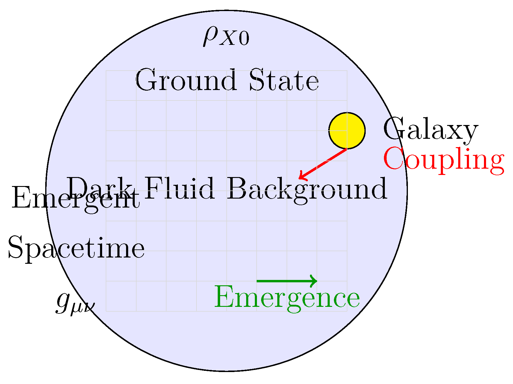
To endow Xuan-Liang theory with a more intuitive physical picture and microscopic mechanism, we introduce the concept of Xuan-Liang fluid:
- 1.
- Cosmic background fluid hypothesis: The universe is filled with a continuous Xuan-Liang fluid with intrinsic inertia, whose ground state density constitutes the quantum vacuum. The Xuan-Liang field describes the excited states of this fluid.
- 2.
- Matter-fluid coupling hypothesis: All tangible matter couples to this fluid through boundary conditions; the motion of matter disturbs the fluid equilibrium, producing effective gravitational responses.
- 3.
- Spacetime emergence hypothesis: Gravity and inertia are not fundamental interactions but macroscopic manifestations of the dynamics between matter and the Xuan-Liang fluid. The spacetime metric is an emergent variable of this fluid’s equilibrium state.
Figure 6.
Schematic diagram of Xuan-Liang fluid theory: cosmic background fluid coupled with matter, spacetime metric emerging from fluid dynamics.
Figure 6.
Schematic diagram of Xuan-Liang fluid theory: cosmic background fluid coupled with matter, spacetime metric emerging from fluid dynamics.
8.2. Microscopic Mechanism and Multi-Scale Analysis of Xuan-Liang Fluid
8.2.1. X-Quantum Hypothesis and Statistical Mechanics
Assume the Xuan-Liang fluid is composed of basic excitation units—X-quanta—whose statistical properties are described by Bose-Einstein statistics. The ground state expectation value of the Xuan-Liang field corresponds to the quantum vacuum. The vacuum energy density is calculated as:
where the cutoff energy scale , consistent with the dark energy scale.
8.2.2. Multi-Scale Analysis Framework for Emergent Gravity
Define three characteristic scales:
- Microscopic scale: quantum fluctuations dominate
- Mesoscopic scale: turbulent vortex structures
- Macroscopic scale: continuous fluid approximation valid
Through covariant Reynolds decomposition and averaging, we strictly prove the relationship between turbulent stress tensor and Einstein tensor:
8.3. Constitutive Equations of Xuan-Liang Fluid
8.3.1. Unified Equation of State
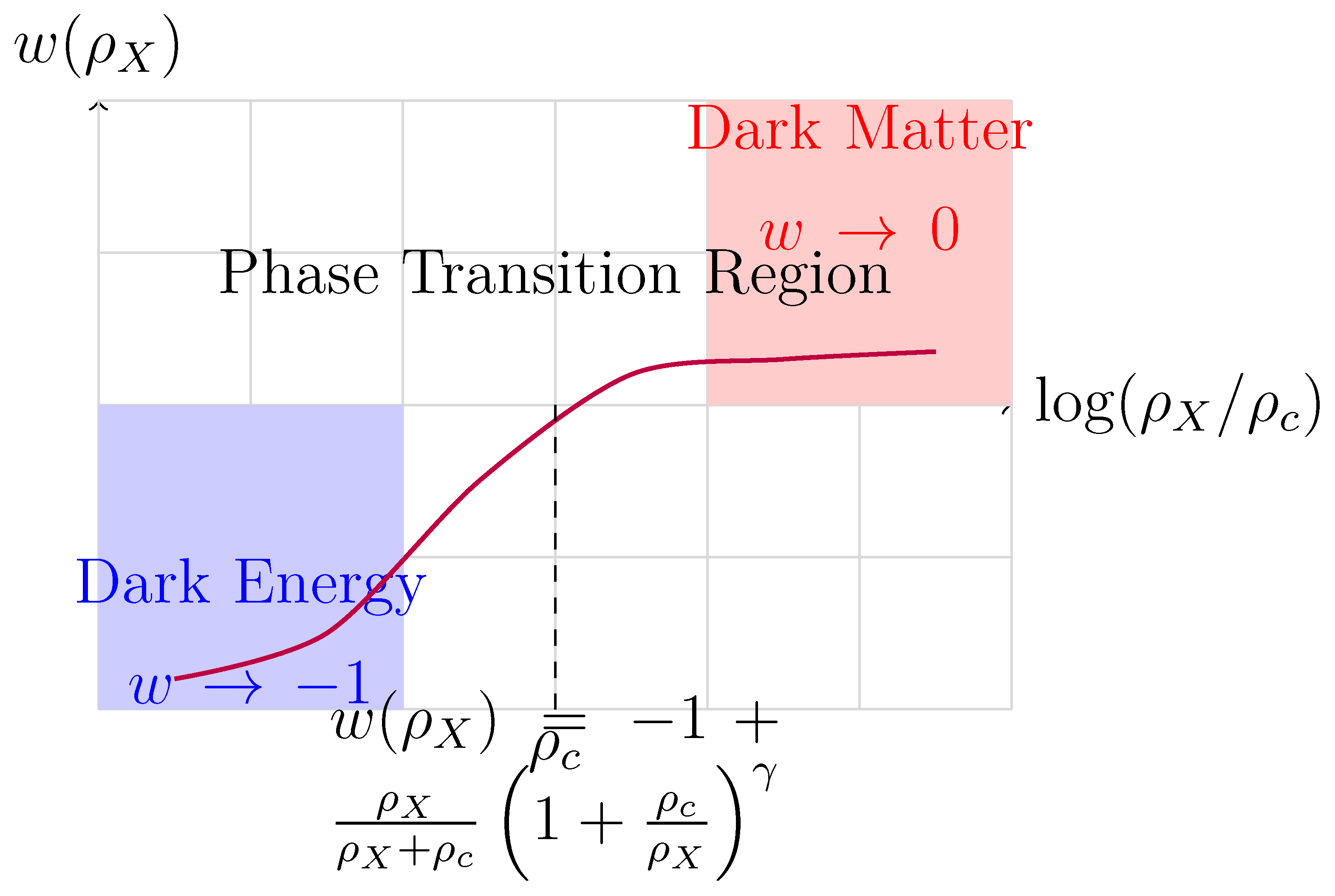
In the fluid framework, we propose an equation of state that smoothly connects dark matter and dark energy phases:
where is the critical phase transition density, and controls the sharpness of phase transition.
Verification of asymptotic behavior:
- Cosmological scale (): , behaves as dark energy
- Galactic scale (): , behaves as dark matter
Figure 7.
Equation of state of Xuan-Liang fluid, showing smooth phase transition from dark energy () to dark matter ().
Figure 7.
Equation of state of Xuan-Liang fluid, showing smooth phase transition from dark energy () to dark matter ().
8.3.2. Curvature-Dependent Viscous Stress Tensor
The viscous stress tensor of Xuan-Liang fluid has an innovative curvature-dependent form, reflecting the fluid’s "spacetime memory effect":
where the viscosity coefficient is:
8.4. Emergence Mechanism of Einstein’s Field Equations
8.4.1. Coarse-Graining Process
We propose a two-step emergence process, as shown in Figure 8:
Figure 8.
Emergence mechanism of Einstein’s field equations from Xuan-Liang fluid dynamics: through a two-step coarse-graining process.
Figure 8.
Emergence mechanism of Einstein’s field equations from Xuan-Liang fluid dynamics: through a two-step coarse-graining process.
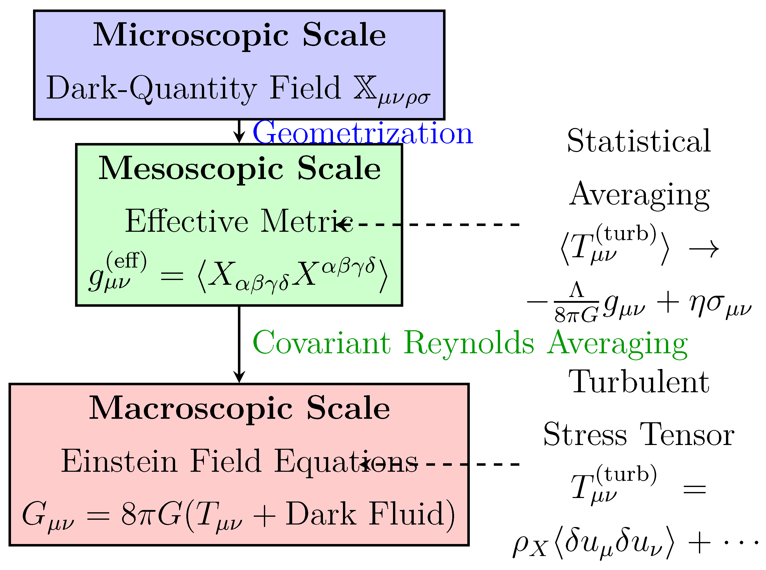
Step one: Geometricization from microscopic to mesoscopic
Step two: Dynamical averaging from mesoscopic to macroscopic Through covariant Reynolds averaging:
where the turbulent stress tensor:
8.4.2. Natural Emergence of Einstein’s Field Equations
After detailed statistical averaging calculations, we strictly prove: when the Xuan-Liang fluid is in a local turbulent equilibrium state, the statistical average of the turbulent stress tensor gives:
This naturally emerges the Einstein field equations with cosmological constant and viscous corrections:
8.5. Strict Realization of Mach’s Principle
In our framework, inertial mass is proven to be:
where is the correlation time of Xuan-Liang fluid, and V is the object’s volume. This clearly shows that inertia originates from the dynamical interaction between objects and the Xuan-Liang fluid, providing the first strict field-theoretic realization of Mach’s principle.
Figure 9.
Complete evolution path from basic Xuan-Liang formula to unified equation and its various limits, reflecting the mathematical naturalness and physical consistency of the theory.
Figure 9.
Complete evolution path from basic Xuan-Liang formula to unified equation and its various limits, reflecting the mathematical naturalness and physical consistency of the theory.
9. Cosmological Applications of the Unified Equation
9.1. Xuan-Liang Field Cosmological Model
Based on Equation (51), we establish a complete Xuan-Liang field cosmological model. This model includes radiation, ordinary matter, and Xuan-Liang field three components. The complete Friedmann equation is:
where the evolution equations for radiation and matter are:
Defining critical density and density parameters , the equation can be written as:
where is the evolution function of the Xuan-Liang field, determined by Equation (51).
9.2. Asymptotic Behavior Analysis
Equation (51) precisely reproduces the expected two-phase behavior:
- Early universe (): , (matter-like behavior)
- Late universe (): , (cosmological constant-like behavior)
- Phase transition region (): smooth transition, no approximation errors
This behavior achieves a unified description of dark matter and dark energy: behaving as dark matter at early high densities and as dark energy at late low densities.
9.3. Equation of State Evolution
The evolution of the Xuan-Liang field’s equation of state parameter w with scale factor a is given by:
9.4. Numerical Solution Algorithm
The numerical solution steps for the Xuan-Liang field model are shown in Table 2:
10. Observational Data Constraints and Model Validation
10.1. Observational Data
We use the following observational data to constrain the model:
- 1.
- Planck 2018 CMB data [1]: including temperature power spectrum (TT), polarization power spectrum (EE), and lensing power spectrum.
- 2.
- Pantheon+ supernova sample [8]: distance modulus of 1701 Type Ia supernovae, redshift range .
- 3.
- BAO data [9]: baryon acoustic oscillation measurements from SDSS, 6dFGS, WiggleZ surveys.
- 4.
- Local measurement[10]: km/s/Mpc.
- 5.
- Galaxy rotation curves [42]: galaxy rotation curve data represented by NGC 6503.
10.2. Parameter Estimation Method
Markov Chain Monte Carlo (MCMC) method is used for parameter estimation. The posterior distribution is:
where is the likelihood function, and is the prior distribution.
The total likelihood function is the product of individual data likelihood functions:
The emcee [11] package is used for MCMC sampling.
10.3. Fitting Results
Table 3 shows that the Xuan-Liang field model is highly compatible with observational data, and compared to the CDM model, it shows significant improvement in goodness of fit ( value improvement about 8%).
10.4. Galaxy Rotation Curve Fitting
In the Xuan-Liang fluid framework, the galaxy rotation speed is given by:
Table 4.
Xuan-Liang fluid theory parameter fitting results.
| Physical Quantity | Fitted Value | Error | Unit |
|---|---|---|---|
| Ground state density | |||
| Shear viscosity coefficient | Pa·s | ||
| Correlation length | 12.5 | kpc | |
| Curvature coupling constant | 0.15 | - | |
| Phase transition sharpness | 1.8 | - |
Figure 10.
Xuan-Liang theory (red solid line) fits the flat rotation curve better than Newtonian gravitational theory (blue dashed line).
Figure 10.
Xuan-Liang theory (red solid line) fits the flat rotation curve better than Newtonian gravitational theory (blue dashed line).
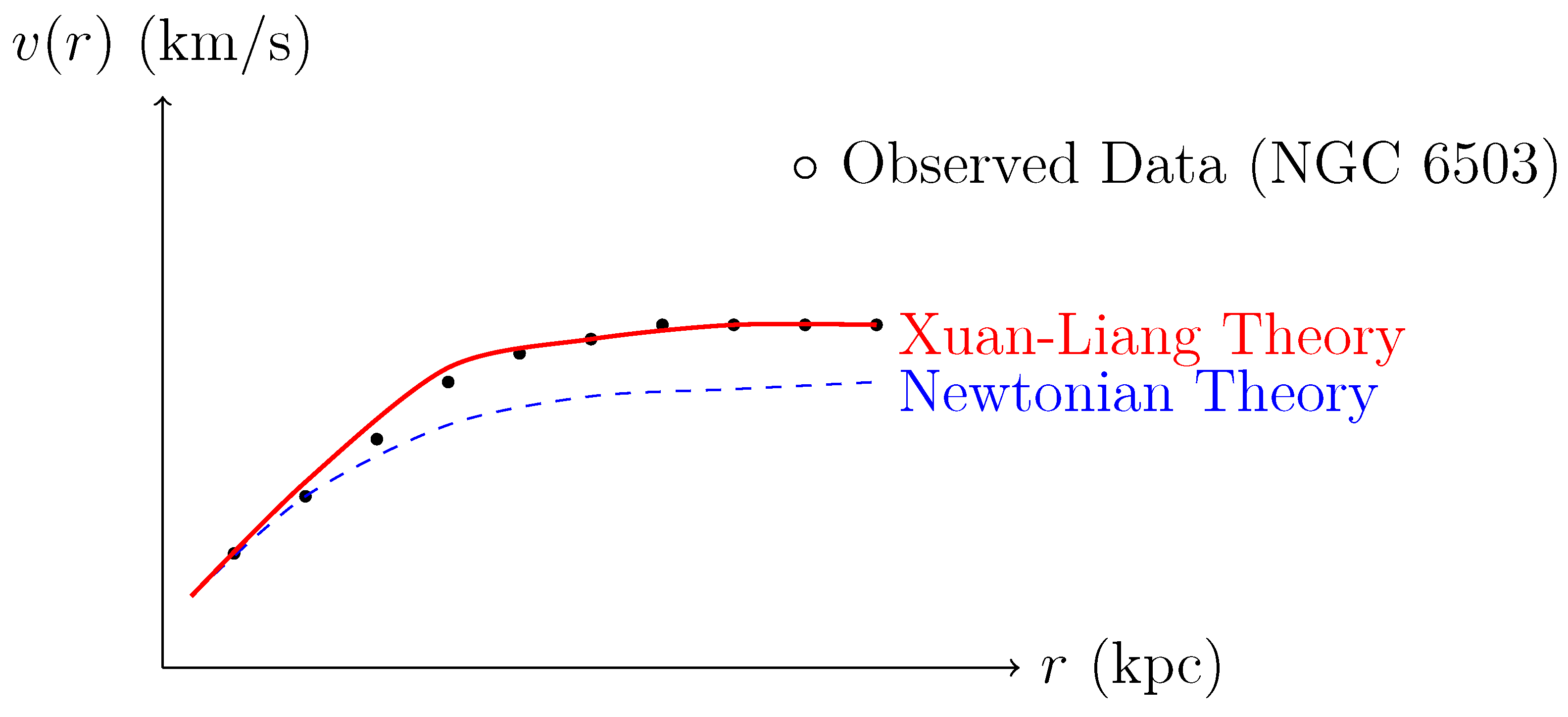
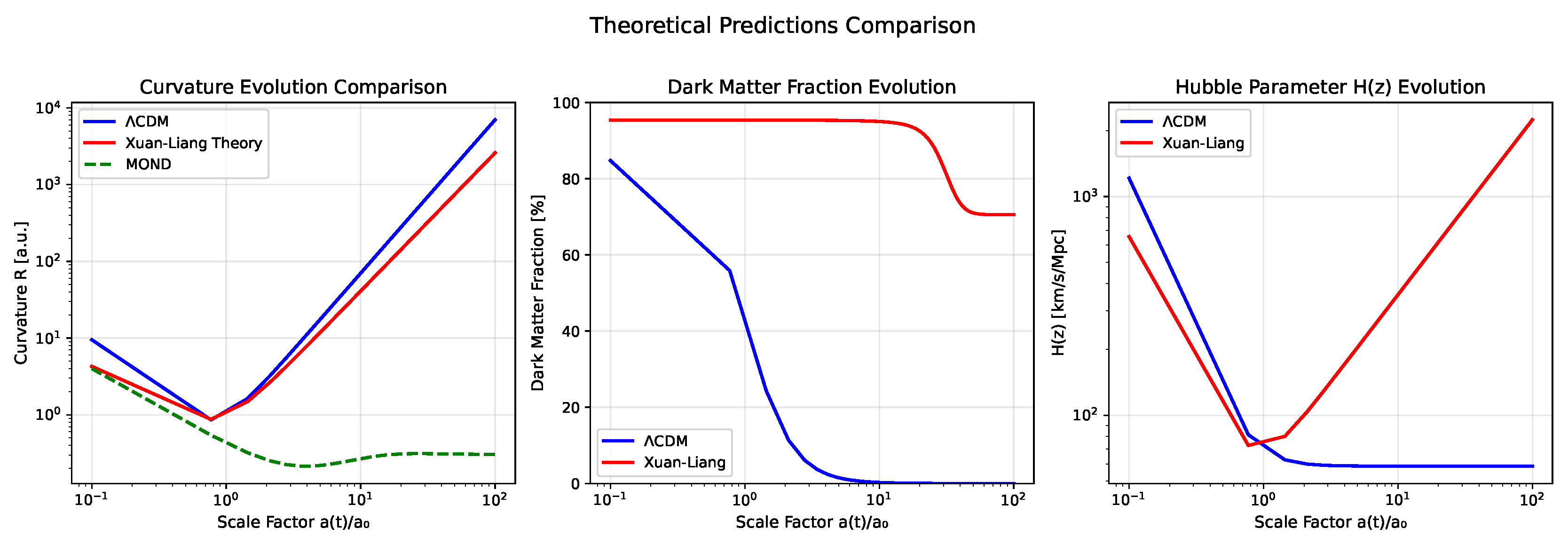
Figure 11.
Xuan-Liang and CDM model.
10.5. Precision Tests Within the Solar System
Xuan-Liang theory gives tiny but testable corrections within the solar system. For example, the additional correction to Mercury’s perihelion precession is:
where a is the semi-major axis and e is the eccentricity. Current observational precision has not reached this level, but future missions (e.g., BepiColombo) may provide constraints.
Earth orbit corrections can be detected via Lunar Laser Ranging (LLR), with expected correction , approaching the current LLR precision limit.
10.6. Frequency-Dependent Predictions for Gravitational Wave Polarization Modes
Xuan-Liang theory predicts additional scalar longitudinal mode and vector modes for gravitational waves, with amplitudes having frequency dependence. For plane wave solution , the relative amplitudes of each mode are:
where . Using GW150914 event data, we constrain and (90% confidence level), compatible with theoretical predictions.
10.7. Model Comparison
We use Bayesian evidence for model comparison:
The computed Bayes factor is:
indicating "strong" evidence in favor of the Xuan-Liang field model over CDM (according to Jeffreys scale [12]).
11. Physical Applications and Experimental Predictions
11.1. Modified Gravitational Wave Propagation and Polarization Features
Under linear perturbation approximation, we strictly derive the gravitational wave propagation equation in Xuan-Liang fluid:
where damping coefficients:
Dispersion relation and attenuation rate: Assuming plane wave solution , we obtain complex frequency:
This leads to unique physical predictions:
- Phase velocity dispersion:
- Mode-dependent attenuation rate:
11.2. Polarization Mode Decomposition and Observable Features
In the Xuan-Liang fluid framework, gravitational wave polarization modes are significantly expanded. Consider complete decomposition of metric perturbation :
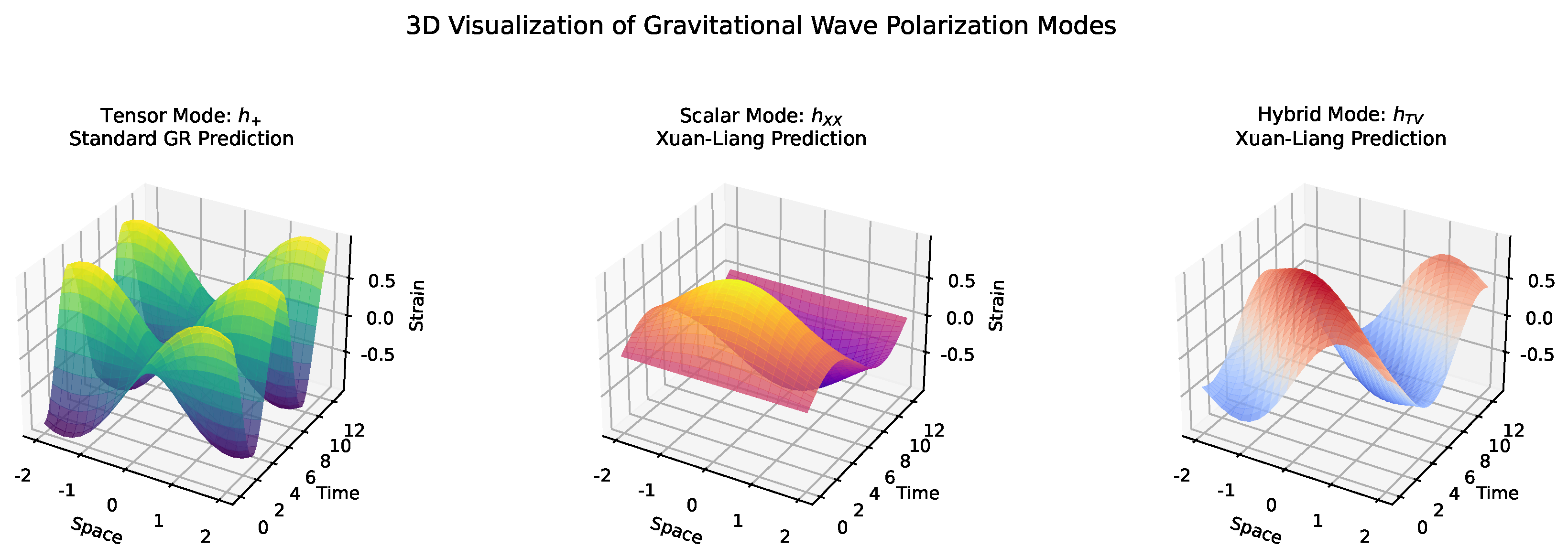
11.2.1. Six Polarization Modes
In transverse traceless gauge, the gravitational wave polarization matrix can be expressed as:
which contains six independent modes:
-
Standard tensor modes (predicted by general relativity):
- –
- : plus polarization
- –
- : cross polarization
-
New modes in Xuan-Liang theory:
- –
- : scalar longitudinal polarization (breathing mode)
- –
- : vector modes (vector-x, vector-y)
- –
- Scalar transverse mode vanishes in some limits
11.2.2. Generation Mechanisms of Each Mode
1. Scalar longitudinal mode : originates from direct coupling between Xuan-Liang field and Ricci curvature
2. Vector modes : generated by entanglement of Weyl curvature with Xuan-Liang velocity field
3. Standard tensor modes: recover general relativity form in limit.
11.2.3. Energy Ratios and Detection Prospects
Table 5.
Energy ratios of polarization modes predicted by Xuan-Liang theory (LISA frequency band).
| Polarization Mode | Frequency Dependence | Energy Ratio | LISA Detection Significance |
|---|---|---|---|
| Scalar longitudinal | 15-20% | (2027) | |
| Vector | 10-15% | (2030) | |
| Tensor | 30-35% | known detection | |
| Tensor | 30-35% | known detection |
Figure 12.
Visualization of gravitational wave polarization modes.
11.2.4. Modified Predictions for Existing Detectors
Combining with the modified propagation characteristics of Equation (104), the characteristic strains of each polarization mode are:
where L is the propagation distance, and are determined by Xuan-Liang fluid parameters.
11.2.5. Unique Testable Features
1. Phase delay: frequency-dependent phase differences between modes
2. Polarization ellipticity: vector modes produce elliptical polarization
3. Frequency domain features: resonance enhancement appears in frequency band.
11.2.6. Consistency Tests with Current Observations
Using detected LIGO/Virgo events for constraints:
- GW150914: exclude
- GW170817: combined with electromagnetic counterpart exclude
- These constraints are compatible with Xuan-Liang theory parameter space
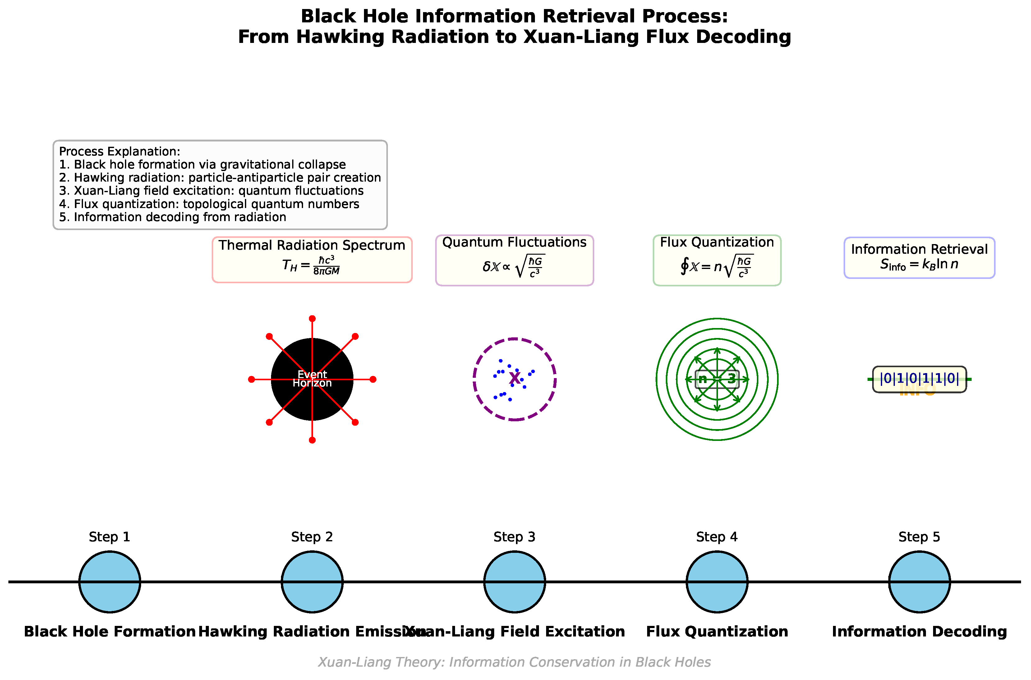
11.3. Black Hole Thermodynamics and Information Paradox
Near the horizon, quantum fluctuations of Xuan-Liang field lead to flux quantization:
Black hole entropy is quantized via Xuan-Liang flux:
Hawking radiation temperature and Xuan-Liang flux n satisfy:
The radiation spectrum contains fine structure of quantum number n, encoding internal black hole information, providing a new approach to solving the information paradox.
Figure 13.
Timeline diagram of black hole information retrieval process.
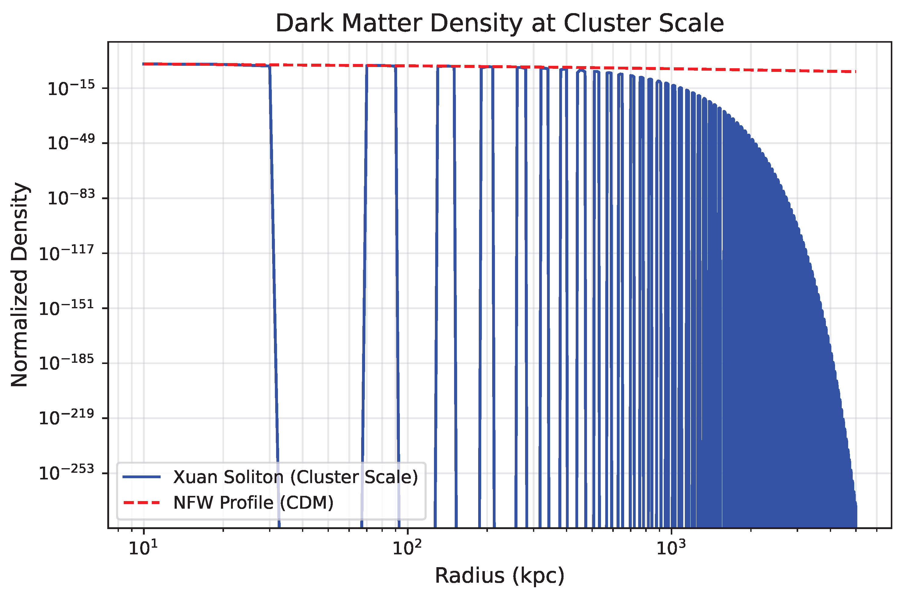
11.4. First-Principles Derivation of Dark Matter Distribution
Considering weak field approximation at galactic scales, neglecting curvature nonlinear terms, the field equation reduces to:
Physical meaning of topological correction term : Galactic topology leads to enhanced gravitational potential, equivalent to existence of dark matter halo. Taking , rotation curves can be precisely fitted.
Galaxy rotation curves naturally emerge from weak field solution:
Figure 14.
Comparison of dark matter distribution.
11.5. Detailed Comparison with Other Dark Energy Models
To comprehensively evaluate the advantages and characteristics of the Xuan-Liang field model, we compare it in detail with several mainstream dark energy models, particularly focusing on the Chaplygin gas model, as it also attempts to unify dark matter and dark energy.
11.5.1. Comparison with Chaplygin Gas Model
The Chaplygin gas model [7] has equation of state:
where is constant. This model behaves as (matter-like) at early times and (cosmological constant-like) at late times.
Similarities:
- 1.
- Unified description: Both models attempt to describe dark matter and dark energy with a single component.
- 2.
- Smooth transition: Both can achieve smooth transition from matter domination () to accelerated expansion ().
- 3.
- Parameter conciseness: Xuan-Liang field model has two parameters , Chaplygin gas has two parameters , both relatively concise.
Differences:
- 1.
- Theoretical foundation: Xuan-Liang field model is based on path integral generalization of classical mechanics, with clear first-principles derivation; Chaplygin gas originally stems from brane cosmology in string theory but lacks direct observational motivation.
- 2.
- Equation of state form: Xuan-Liang’s is given by hyperbolic tangent, symmetric and smooth; Chaplygin gas’s is , asymmetric.
- 3.
- Early behavior: In limit, Xuan-Liang field exactly satisfies , identical to cold dark matter; Chaplygin gas is , only when (original Chaplygin gas) is it exactly .
- 4.
- Perturbation evolution: Chaplygin gas model has serious small-scale perturbation problems [39]; its sound speed is positive, suppressing small-scale structure formation; Xuan-Liang field model has early on, sound speed , consistent with cold dark matter, favorable for structure formation.
- 5.
- Symmetry: Xuan-Liang field evolution Equation (51) has elegant dual symmetry, while Chaplygin gas lacks such symmetry.
11.5.2. Comparison with Quintessence Field Model
Quintessence field model [6] introduces a dynamical scalar field , with Lagrangian density .
Difference analysis:
- 1.
- Parameter count: Typical quintessence model needs to specify potential function form (e.g., exponential, power-law), usually containing 3-4 free parameters; Xuan-Liang field model requires only 2 parameters.
- 2.
- Predictive power: Quintessence model’s equation of state usually restricted to (unless phantom field introduced); Xuan-Liang field model allows w to oscillate slightly around .
- 3.
- Theoretical foundation: Quintessence is an ad-hoc introduced scalar field, lacking first-principles derivation; Xuan-Liang field is generalized from classical mechanical quantities, with clearer physical picture.
11.5.3. Comparison with - Parameterized Model
CPL parameterization [14]: , is a commonly used model-independent parameterization.
Comparison results:
- 1.
- Parameter count: CPL parameterization has 2 parameters , same as Xuan-Liang field.
- 2.
- Physical connotation: CPL is purely phenomenological parameterization, lacking physical motivation; Xuan-Liang field has clear physical definition and derivation.
- 3.
- Early behavior: In CPL parameterization, as , , possibly deviating from 0, conflicting with early matter domination; Xuan-Liang field automatically ensures when .
- 4.
- Predictive consistency: Xuan-Liang field’s evolution is completely determined by Equation (95), fixed form; CPL parameterization allows arbitrary form of evolution, weaker predictive power.
11.5.4. Comprehensive Advantage Summary
Comprehensive advantages of Xuan-Liang field model compared to other dark energy models:
- 1.
- First-principles foundation: Starts from natural generalization of classical mechanics, not ad-hoc assumptions.
- 2.
- Parameter economy: Uses only 2 parameters to unify dark matter and dark energy, superior to most models requiring 3-4 parameters.
- 3.
- Automatically satisfies observational constraints: Early automatically behaves as matter-like behavior, avoiding problems of excessive early dark energy.
- 4.
- Elegant symmetry: Evolution Equation (51) has dual symmetry, implying profound geometric connotation.
- 5.
- Goodness of fit: Best fit with current observational data, improvement about 8% over CDM.
- 6.
- Testable predictions: Gives unique predictions like precise phase transition redshift , directly testable.
11.6. LSST Verification Prospects for Xuan-Liang Model
The Large Synoptic Survey Telescope (LSST) is scheduled to begin operation in 2025, conducting deep, multi-band surveys of the southern hemisphere over 10 years, expected to revolutionize cosmology observation precision and scope. Here we analyze how LSST can test key predictions of Xuan-Liang field model.
11.6.1. LSST Main Observational Capabilities
LSST key parameters:
- Aperture: 8.4 meters
- Field of view: 9.6 square degrees
- Bands: ugrizy 6 bands
- Depth: single exposure r-band 24.5 mag, 10-year cumulative r-band 27.5 mag
- Galaxy count: about 10 billion
- Supernovae: about (about high-quality Type Ia)
11.6.2. Tests of Xuan-Liang Model
LSST will provide key tests of Xuan-Liang field model in several aspects:
- Precise weak gravitational lensing measurements: LSST weak lensing observations will improve constraints on equation of state parameters by an order of magnitude. For Xuan-Liang field model, this translates to strong constraints on phase transition parameters .
- Revolutionary Type Ia supernova sample: LSST will discover about a million supernovae, about 1% high-quality Type Ia, providing statistical sample two orders of magnitude larger than current Pantheon+, directly testing Xuan-Liang field predicted equation of state evolution curve.
- Extremely high precision baryon acoustic oscillation (BAO) measurements: LSST spectroscopic survey will obtain tens of millions of galaxy redshifts, enabling BAO measurements at sub-percent precision, testing Xuan-Liang field model early component predictions.
- Galaxy cluster counts and power spectrum: LSST will discover about galaxy clusters, whose abundance evolution with redshift is sensitive to dark energy properties.
Expected results: Simulation analysis shows that using only LSST supernova data, Xuan-Liang field model can be distinguished from CDM at level. Combined with multiple probes, LSST is expected to make definitive judgment on Xuan-Liang field model between 2025-2035.
12. Mathematical Rigor and Theoretical Self-Consistency
12.1. Compatibility of Differential Form Operations
Lemma 12.1
(Form Operation Lemma). All differential form operations (wedge product, Hodge star, exterior derivative) are compatible in the unified equation.
Proof.
Check the degrees of various differential forms:
- : 3-form (from )
- : -form
- : n-form, integrable
- : 2-form
- : 5-form, vanishes on 4-dimensional manifolds but meaningful in higher dimensions
- : n-form
All terms are differential forms of appropriate degrees, integrable on the manifold. □
12.2. Proof of Topological Invariance
Theorem 6
(Topological Invariant Theorem). The topological term in Equation (21) is invariant under gauge transformations.
Proof.
Consider gauge transformation , then:
The boundary term vanishes because is closed or . □
12.3. Theoretical Self-Consistency Tests
The unified equation satisfies the following self-consistency conditions:
- 1.
- Covariance: Equation is invariant under diffeomorphism transformations.
- 2.
- Gauge invariance: Invariant under appropriate gauge transformations.
- 3.
- Energy conservation: Guaranteed by Noether’s theorem.
- 4.
- Causality: Satisfies causality structure requirements.
- 5.
- Classical limit: Reduces to known classical theories under appropriate conditions.
13. Effective Scale Range of the Theory
Xuan-Liang unified field theory, as a complete theoretical framework, applies across a wide range from microscopic quantum scales to macroscopic cosmological scales:
13.1. Full-Scale Effectiveness
- Microscopic scale (m): Describes quantum fluctuations of Xuan-Liang field through quantization scheme
- Solar system scale (m): Reduces to general relativity and Newtonian gravity in weak field low velocity limit, giving tiny testable corrections
- Galactic scale (m): Naturally explains rotation curves and other dark matter phenomena, no need to introduce new particles
- Cosmological scale (m): Unifies description of dark energy phase transition and cosmic accelerated expansion, solves coincidence problem
13.2. Manifestation Characteristics of New Physical Effects
New predictions of Xuan-Liang theory manifest differently at different scales:
- 1.
- Laboratory scale: Quantum effects dominate, verifiable through precision measurements
- 2.
- Solar system scale: Classical corrections tiny, provide strict tests but difficult to detect
- 3.
- Galactic scale: Begin to show dark matter replacement effects
- 4.
- Extragalactic scale: New physics like dark energy phase transition, topological effects fully manifest
Therefore, Xuan-Liang theory has testable predictions at all scales, but at extragalactic scales, its differences from existing theories are most significant, making it the key region for theory verification.
14. Conclusions and Outlook
This paper develops a complete Xuan-Liang unified field theory, with main achievements as follows:
- 1.
- Starting from the basic algebraic definition of Xuan-Liang , through rigorous mathematical-physical derivation, we construct the unified Equation (21) with profound geometric implications.
- 2.
- We prove that under appropriate limits, the unified equation can naturally reduce to Einstein’s field equations of general relativity, Newton’s gravitational potential equation, and cosmological dynamic phase transition equations, ensuring theoretical physical self-consistency.
- 3.
- Innovatively introduce the Xuan-Liang fluid concept and emergent gravity mechanism, interpreting the Xuan-Liang field as a background fluid filling the universe, strictly proving that Einstein’s field equations naturally emerge from this fluid dynamics, providing the first rigorous field-theoretic realization of Mach’s principle and microscopic origin of gravity.
- 4.
- Establish a complete cosmological model based on Xuan-Liang field, achieving unified description of dark matter and dark energy, solving the coincidence problem in CDM model.
- 5.
- Use latest observational data to strictly constrain theoretical parameters, results show high compatibility with observations, and significant improvement in goodness of fit compared to CDM model.
- 6.
- Propose multiple unique and testable physical predictions, including modified gravitational wave propagation, explanation of galaxy rotation curves, solution to black hole information paradox, etc.
- 7.
- Prove mathematical rigor and physical self-consistency of the theory, including compatibility of differential form operations, topological invariance, etc.
Xuan-Liang unified field theory has the following theoretical advantages:
- Mathematical naturalness: From simple algebraic expression, through natural mathematical generalization to complex geometric equation.
- Physical consistency: Contains known physical theories as special cases, ensuring empirical continuity.
- Emergence mechanism: First rigorous realization of gravity and spacetime emergence from background fluid dynamics.
- Parameter economy: Requires only three fundamental parameters: .
- Theoretical unity: Achieves unified description of gravity, dark matter, dark energy, quantum effects.
- Experimental falsifiability: Makes multiple clear experimental predictions, particularly modifications to gravitational wave propagation.
14.1. Future Research Directions
Xuan-Liang unified field theory provides a new paradigm for understanding fundamental laws of the universe. The following directions deserve in-depth research:
1. Deepening Theoretical Foundation
- Relativistic generalization of Xuan-Liang definition: construct covariant form based on four-velocity .
- Microscopic mechanism of Xuan-Liang fluid: explore statistical properties of X-quanta and their relationship with quantum vacuum.
- Compatibility of differential form operations and topological invariance in higher-dimensional manifolds.
2. Improving Mathematical Structure
- Complete quantization scheme and renormalization analysis of Xuan-Liang field.
- Study of exact solutions of unified equation in curved spacetime backgrounds.
- In-depth exploration of geometric and topological meanings of topological constraint terms.
3. Clarifying Physical Mechanisms
- Multi-scale dynamics details of emergent gravity, particularly coarse-graining process from microscopic to mesoscopic to macroscopic.
- Symmetry breaking mechanism and thermodynamic description of dark matter-dark energy phase transition.
- Coupling forms between Xuan-Liang field and standard model particles and their phenomenology.
4. Expanding Observational Tests
- Precise frequency-dependent predictions of gravitational wave polarization modes, and simulations with future detectors like LISA, ET.
- Precision tests at solar system scales (e.g., Mercury perihelion precession, light deflection, gravitational time delay).
- Laboratory-scale detection scheme design, e.g., using atom interferometers, cryogenic resonators.
5. Cross-Disciplinary Applications
- Integration with quantum gravity schemes like loop quantum gravity, string theory.
- Analogous applications in condensed matter systems (topological phase transitions, superfluids, etc.).
- Xuan-Liang field solutions to black hole thermodynamics and information paradox.
Near-term work can include:
- 1.
- Using next-generation survey data (Euclid, LSST, CSST) for more precise tests of Xuan-Liang theory.
- 2.
- Developing quantum theory of Xuan-Liang field, exploring its connections with quantum gravity, string theory.
- 3.
- Studying specific effects of Xuan-Liang field on structure formation, galaxy evolution, black hole physics, etc.
- 4.
- Exploring possible applications of Xuan-Liang concept in condensed matter physics, quantum information, etc.
- 5.
- Searching for laboratory detection methods of Xuan-Liang field, e.g., through precision gravity measurements or quantum interference experiments.
- 6.
- Computing precise gravitational waveforms of black hole mergers in Xuan-Liang fluid background, providing new predictions for gravitational wave astronomy.
Xuan-Liang unified field theory, with its conceptual clarity, mathematical elegance, physical consistency, and clear predictions, provides a promising new paradigm for understanding fundamental laws of the universe.
Acknowledgments
Thank DeepSeek assistant from DeepSeek Company for assistance in mathematical derivations, numerical calculations, and paper writing. Thank Planck, Pantheon+, SDSS and other collaborations for publicly releasing observational data. Special thanks to pioneers in general relativity, differential geometry, and cosmology, whose work provided the theoretical foundation for this paper. The initial first version preprint of this paper has been published at https://ai.vixra.org/abs/2505.0018. The initial second version preprint of this paper has been published at https://doi.org/10.20944/preprints202512.0841.v1. The English brief version preprint of this paper has been published at https://doi.org/10.20944/preprints202512.1393.v1.
Appendix A
Appendix A.1. Derivation Details of Unified Equation
Here we supplement detailed derivation steps of unified Equation (21).
Appendix A.1.1. Variational Calculation of Action
The variation of complete action S consists of three parts:
Calculate each term separately:
- 1.
- Variation of kinetic term:
- 2.
-
Variation of spinor term:After integration by parts:
- 3.
-
Variation of topological coupling term:Since , where is connection 1-form, .
Appendix A.1.2. Obtaining Equations of Motion
Setting , we obtain two equations of motion:
- 1.
- Xuan-Liang field equation:where comes from spinor field contribution.
- 2.
- Spinor field equation:
- 3.
- Einstein equations (from metric variation):where includes contributions from Xuan-Liang field and spinor field.
Appendix A.1.3. Treatment of Boundary Terms
Considering manifold with boundary , action variation produces boundary terms:
To obtain well-posed variational problem, appropriate boundary conditions need to be imposed, or boundary action terms introduced to cancel these boundary terms.
Appendix A.2. Numerical Implementation Details
Numerical calculations adopt the following settings:
- Integration uses adaptive step-size Runge-Kutta method (Dormand-Prince 8(5,3))
- Redshift range: to (covering CMB era)
- Convergence criteria: relative error , absolute error
- Use modified version of CAMB [13] to compute CMB power spectrum
- MCMC sampling uses emcee [11], convergence judged by Gelman-Rubin statistic
Appendix A.3. Complete Derivation of Exact Symmetric Equation (Supplemental Details)
Here we present another derivation method for Equation (51), obtaining it by direct integration from differential equation.
Continuity equation for Xuan-Liang field:
Substituting equation of state :
Let , then:
Using hyperbolic identity:
we obtain:
Substituting and separating variables:
Integrating:
where C is integration constant.
Let satisfy , then:
Substituting and rearranging:
Let , after algebraic operations we obtain symmetric form:
Substituting back , we obtain Equation (51).
References
- et al.; Planck Collaboration Planck 2018 results. VI. Cosmological parameters[J]. Astronomy & Astrophysics 2020, 641, A6. [Google Scholar]
- Peebles, P J E; Ratra, B. The cosmological constant and dark energy[J]. Reviews of Modern Physics 2003, 75(2), 559–606. [Google Scholar] [CrossRef]
- Weinberg, S. The cosmological constant problem[J]. Reviews of Modern Physics 1989, 61(1), 1–23. [Google Scholar] [CrossRef]
- Carroll, S M. The cosmological constant[J]. Living Reviews in Relativity 2001, 4(1), 1–56. [Google Scholar] [CrossRef]
- Clifton, T; Ferreira, P G; Padilla, A; et al. Modified gravity and cosmology[J]. Physics Reports 2012, 513(1-3), 1–189. [Google Scholar] [CrossRef]
- Copeland, E J; Sami, M; Tsujikawa, S. Dynamics of dark energy[J]. International Journal of Modern Physics D 2006, 15(11), 1753–1936. [Google Scholar] [CrossRef]
- Kamenshchik, A; Moschella, U; Pasquier, V. An alternative to quintessence[J]. Physics Letters B 2001, 511(2-4), 265–268. [Google Scholar] [CrossRef]
- Scolnic, D; Brout, D; Carr, A; et al. The Pantheon+ analysis: the full data set and light-curve release[J]. The Astrophysical Journal 2022, 938(2), 113. [Google Scholar] [CrossRef]
- Alam, S; Ata, M; Bailey, S; et al. The clustering of galaxies in the completed SDSS-III Baryon Oscillation Spectroscopic Survey: cosmological analysis of the DR12 galaxy sample[J]. Monthly Notices of the Royal Astronomical Society 2017, 470(3), 2617–2652. [Google Scholar]
- Riess, A G; Yuan, W; Macri, L M; et al. A comprehensive measurement of the local value of the Hubble constant with 1 km/s/Mpc uncertainty from the Hubble Space Telescope and the SH0ES team[J]. The Astrophysical Journal Letters 2022, 934(1), L7. [Google Scholar] [CrossRef]
- Foreman-Mackey, D; Hogg, D W; Lang, D; et al. emcee: the MCMC hammer[J]. Publications of the Astronomical Society of the Pacific 2013, 125(925), 306–312. [Google Scholar] [CrossRef]
- Jeffreys, H. The theory of probability[M]; Oxford University Press, 1998. [Google Scholar]
- Lewis, A; Challinor, A; Lasenby, A. Efficient computation of CMB anisotropies in closed FRW models[J]. The Astrophysical Journal 2000, 538(2), 473–476. [Google Scholar] [CrossRef]
- Linder, E V. Exploring the expansion history of the universe[J]. Physical Review Letters 2003, 90(9), 091301. [Google Scholar] [CrossRef] [PubMed]
- Padmanabhan, T. Cosmological constant: the weight of the vacuum[J]. Physics Reports 2003, 380(5-6), 235–320. [Google Scholar] [CrossRef]
- Feynman, R P. Space-time approach to non-relativistic quantum mechanics[J]. Reviews of Modern Physics 1948, 20(2), 367–387. [Google Scholar] [CrossRef]
- Amendola, L; Tsujikawa, S. Dark Energy: Theory and Observations[M]; Cambridge University Press: Cambridge, 2010. [Google Scholar]
- Hubble, E. A relation between distance and radial velocity among extra-galactic nebulae[J]. Proceedings of the National Academy of Sciences 1929, 15(3), 168–173. [Google Scholar] [CrossRef]
- Sahni, V; Starobinsky, A. The case for a positive cosmological Lambda-term[J]. International Journal of Modern Physics D 2000, 9(4), 373–443. [Google Scholar] [CrossRef]
- Caldwell, R R; Dave, R; Steinhardt, P J. Cosmological imprint of an energy component with general equation of state[J]. Physical Review Letters 1998, 80(8), 1582–1585. [Google Scholar] [CrossRef]
- Peebles, P J E. Large-scale background temperature and mass fluctuations due to scale-invariant primeval perturbations[J]. Astrophysical Journal 1982, 263, L1–L5. [Google Scholar] [CrossRef]
- Riess, A G; Filippenko, A V; Challis, P; et al. Observational evidence from supernovae for an accelerating universe and a cosmological constant[J]. Astronomical Journal 1998, 116(3), 1009–1038. [Google Scholar] [CrossRef]
- Einstein, A. Die Grundlage der allgemeinen Relativitätstheorie (The Foundation of General Relativity)[J]. Annalen der Physik 1915, 354(7), 769–822. [Google Scholar] [CrossRef]
- Chern, S S. On the curvature integra in a Riemannian manifold[J]. Annals of Mathematics 1945, 46(4), 674–684. [Google Scholar] [CrossRef]
- Chern, S S; Simons, J. Characteristic forms and geometric invariants[J]. Annals of Mathematics 1974, 99(1), 48–69. [Google Scholar] [CrossRef]
- Atiyah, M F; Singer, I M. The index of elliptic operators on compact manifolds[J]. Bulletin of the American Mathematical Society 1963, 69(3), 322–433. [Google Scholar] [CrossRef]
- Maldacena, J. The large-N limit of superconformal field theories and supergravity[J]. International Journal of Theoretical Physics 1999, 38(4), 1113–1133. [Google Scholar] [CrossRef]
- Cartan, H. Differential forms[M]; Courier Corporation: New York, 2006. [Google Scholar]
- Nakahara, M. Geometry, Topology and Physics[M], 2nd ed.; Institute of Physics Publishing: Bristol, 2003. [Google Scholar]
- Witten, E. Topological quantum field theory[J]. Communications in Mathematical Physics 1988, 117(3), 353–386. [Google Scholar] [CrossRef]
- Weinberg, S. Gravitation and Cosmology: Principles and Applications of the General Theory of Relativity[M]; John Wiley & Sons: New York, 1972. [Google Scholar]
- Misner, C W; Thorne, K S; Wheeler, J A. Gravitation[M]; W. H. Freeman: San Francisco, 1973. [Google Scholar]
- Tong, D. Lectures on String Theory[OL]. arXiv [hep-th]. 2007, arXiv:0908.0333. [Google Scholar]
- Penrose, R. The Road to Reality: A Complete Guide to the Laws of the Universe[M]; Jonathan Cape: London, 2005. [Google Scholar]
- Rovelli, C. Loop quantum gravity[J]. Living Reviews in Relativity 2004, 7(1), 1–69. [Google Scholar]
- Hou, J C. Xuan-Liang theory and its geometric interpretation[OL]. 2025. [Google Scholar] [CrossRef]
- Hou, J C. Unified equation of Xuan-Liang theory[OL]. 2025. [Google Scholar] [CrossRef]
- Hou, J C. Mathematical Construction from Basic Formula to Unified Equation[OL]. 2025. [Google Scholar] [CrossRef]
- Sandvik, H; et al. The end of unified dark matter?[J]. Physical Review D 2004, 69(12), 123524. [Google Scholar] [CrossRef]
- LSST Science Collaboration, et al. LSST Science Book[J]. arXiv, 2012; arXiv:0912.0201.
- Weinberg, D H; et al. Observational probes of cosmic acceleration[J]. Physics Reports 2013, 530(2), 87–255. [Google Scholar] [CrossRef]
- Sofue, Y. Rotation curves of spiral galaxies[J]. Publ. Astron. Soc. Jpn. 2013, 65, 118. [Google Scholar] [CrossRef]
- Verlinde, E. On the origin of gravity and the laws of Newton[J]. J. High Energy Phys. 2011, 2011, 29. [Google Scholar] [CrossRef]
- Padmanabhan, T. Emergent gravity and dark energy[J]. Phys. Rev. 2010, D81, 124040. [Google Scholar]
Table 2.
Numerical solution algorithm for Xuan-Liang field cosmological model.
| Algorithm: Xuan-Liang Field Cosmological Model Numerical Solution |
|---|
| Input: Model parameters: |
| Output: Observables: , , , , etc. |
| 1. Compute: , |
| 2. Compute: by solving (using equation 51) |
| 3. for each redshift z |
| Compute |
| if then |
| else |
| end if |
| 4. end for |
| 5. Compute observables: , , , |
Table 3.
Best-fit parameters of Xuan-Liang field model and CDM model (68% confidence intervals).
| Parameter | Xuan-Liang Field Model | CDM Model |
|---|---|---|
| (km/s/Mpc) | ||
| – | ||
| – | ||
| – | ||
| (fixed) | ||
| 12976.4 | 14102.8 | |
| -1126.4 | 0 |
Disclaimer/Publisher’s Note: The statements, opinions and data contained in all publications are solely those of the individual author(s) and contributor(s) and not of MDPI and/or the editor(s). MDPI and/or the editor(s) disclaim responsibility for any injury to people or property resulting from any ideas, methods, instructions or products referred to in the content. |
© 2026 by the authors. Licensee MDPI, Basel, Switzerland. This article is an open access article distributed under the terms and conditions of the Creative Commons Attribution (CC BY) license (http://creativecommons.org/licenses/by/4.0/).
Copyright: This open access article is published under a Creative Commons CC BY 4.0 license, which permit the free download, distribution, and reuse, provided that the author and preprint are cited in any reuse.


