Submitted:
13 December 2025
Posted:
15 December 2025
You are already at the latest version
Abstract
Financial time series often show periods where market index values or asset prices increase or decrease monotonically.These events are known as price runs, uninterrupted trends, or simply runs. By identifying such runs in the daily DJIA and IPC indices from 01/02/1990 to 10/17/2025, we construct their associated returns, to obtain a non-arbitrary sample of multi-scale returns, we named trend returns (TReturns). The time scale for each multi-scale return is determined by the exponentially distributed duration of its respective run. We empirically reveal that the distribution of these coarse-grained returns show interesting statistical properties: the central region displays an exponential decay, likely resulting from the exponential trend duration, while the tails follow a power-law decay. This combination of exponential central behavior and asymptotic power-law decay has also been observed in other complex systems; and our findings provide an additional evidence of its natural emergence. We also explore the informational aspects of multi-scale returns using three measures: Shannon entropy, permutation entropy and compression-based complexity. We find that Shannon entropy increases with coarse-graining, indicating a wider range of values; permutation entropy drops sharply, revealing underlying temporal patterns and compression ratios improve, reflecting suppresed randomness. Overall, these findings suggest that constructing TReturns filters out microscopic noise, reveals structureded temporal patterns, and provides a complementary and clear view of market behavior.
Keywords:
price runs
; market efficiency
; multi-scale returns properties
; empirical analysis
1. Introduction
Since the late eighteenth century, the success of the Physical Sciences inspired economists, specially within the Neoclassical tradition, to build economic theory following the methodological structure of Physics, and in particular Analytical Mechanics [1]. In this sense, Physics and Mathematics have long played a central role in shaping the development of the Economic Sciences.
Since the mid 1990s, challenging problems arising in economic and social systems began to attract growing interest from the Physics community. This effort gave rise to Econophysics, a field where techniques from computational statistical mechanics are applied to economic systems from both theoretical and empirical perspectives. Over time, researchers from Computer Science, Biology, Big Data, Artificial Intelligence and related fields joined this movement, approaching economic phenomena with both applied and foundational goals. The broader research area that studies systems composed of large numbers of particles or agents using interdisciplinary tools is now commonly referred to as the Complexity Sciences.
Due to their nature, economic and social systems cannot be easily manipulated through controlled experiments. Nevertheless the massive growth of computational power, together with the availability of large datasets accumulated over decades, and in some cases centuries, has opened the door to an empirical and quasi-experimental approach to socio-economic phenomena. Rich data sources now include financial prices, transaction records, personal income archives, large-scale surveys, and, more recently, vast datasets extracted from social networks that capture information on human interactions, preferences, opinions and political behavior.
In this paper, following an empirical methodology rooted in Econophysics, we analyze the financial time series of two market indices: the American Dow Jones Industrial Average (DJIA) and the Mexican Stock Exchange Index (IPC), described in detail in Section 4.
1.1. Stylized Facts
Under this empirical standpoint, several non-trivial and remarkably universal statistical properties of financial time series, known as stylized facts, have been documented. Although often formulated in qualitative terms, these properties impose rigorous constraints on any statistical description, and reproducing all of them simultaneously remains very challenging for standard stochastic models [2]. As far as we know, no existing theory or model is currently able to explain the origin of all stylized facts together. However, agent-based modeling has been suggested as a promising methodological way to address this limitation [3,4,5]. This view is reinforced by recent developments in kinetic and microstructural modeling [6,7] and by the broader econophysics literature, where stylized facts are recognized as signatures of complex-system behavior [8].
Interestingly, stylized facts appear not only in financial markets but also in other complex dynamical systems, sometimes surprisingly simple ones, such as Conway’s Game of Life [9].
We summarize below some of the most relevant stylized facts [2]:
- Heavy tails:
- Return distributions are leptokurtic and exhibit asymptotic power-law decay.
- Absence of linear autocorrelations:
- Autocorrelations of returns are negligible except at very short time scales, depending on the market and sampling frequency.
- Gain–loss asymmetry:
- Large downward movements in stock prices or indices are more frequent than equally large upward movements.
- Volatility clustering:
- Periods of high volatility tend to cluster in time.
- Other:
- Additional properties include aggregational Gaussianity, volume/volatility correlations, long memory in autocorrelation of absolute returns and many more.
1.2. Coexistence of Joint Exponential and Power-Law Distributions Across Diverse Complex Systems
Although the stylized facts concept is primarily a financial term, several statistical properties appear not only in financial markets but across a wide range of complex systems. A recurring statistical pattern in complex systems is the coexistence of an exponential central region and asymptotic power-law tails. This pattern appears in settings with radically different microscopic rules and physical substrates: the distribution of wealth and income follows an exponential law in the low and central regions with heavy-tailed extremes in all societies [10]; cultural ranking processes, such as the Dutch Top 2000 pop-song list [11]; cellular automaton “the Game of Life”, generate thermal and superthermal wealth-like distributions [12]; suprathermal particle populations in space and atmospheric plasma [13,14,15]; hydrodynamic extensions of hadronic production models in heavy-ion collisions [16]; the autocorrelation envelopes of multi-scale financial returns [17], etc. This recurrence of the same statistical form across socioeconomic systems, astrophysical plasmas, cellular automata, cultural dynamics and high-energy physics suggests a microscopic organizational principle that gives rise to the previously mentioned statistical patterns. Although a unified theory explaining why this combination arises still remains to be developed, the empirical regularity is indisputable and clear. We mention these examples because in this paper, we add yet another instance of the joint emergence of these two distributions in a complex system. The stochastic process introduced here, the multi-scale returns is itself governed by the same distribution exponential in the central region and decays as an asymptotic power-law in the tails, just as the systems mentioned above.
2. Data Sample
The data analyzed in this work consist of the daily closing values of two financial indices: the American Dow Jones Industrial Average (DJIA) and the Mexican Price and Quotations Index (IPC, Índice de Precios y Cotizaciones), covering the period from January 2, 1990 to October 17, 2025.
The IPC series was initially obtained from historical datasets provided to us by the Bolsa Mexicana de Valores (BMV) for academic use , and from datasets that were publicly accessible at the time from the Bank of Mexico. These historical records were later complemented with additional public sources to construct a continuous and internally consistent IPC dataset.
For the DJIA series, publicly accessible historical records were used, including datasets available at the time from the Central Bank of Brazil. The data was publicly accessible when retrieved by the authors, as it was originally downloaded from diverse public portals, some of which subsequently withdrew their corresponding historical files. Both the IPC and DJIA series, required further preprocessing to address common issues found in long financial time series, such as repeated dates, duplicated rows, inconsistent timestamps, and entries for non-trading days. After the full cleaning and reconstruction procedure, the IPC and DJIA datasets consisted of 8,996 and 9,011 daily observations, respectively.
The final reconstructed datasets used in this study, together with all derived observables analyzed in the following sections, are publicly available in the companion Zenodo repository: https://doi.org/10.5281/zenodo.17781871.
Below, we describe how the observables analyzed in this work are constructed from the two datasets.
3. Methodology and Construction of the Multi-Scale Returns
The evolution of an asset price on a time-series chart, often reveals periods during which the price (or index value) increases or decreases monotonically. We refer to these periods as runs, uninterrupted price trends or simply trends. These alternating upward and downward movements form the foundation of our construction of multi-scale returns. For illustration, Figure 1 shows examples of uninterrupted trends in the DJIA during an earlier period November/03/2003 - January/13/2004.
More formally, let denote the time series of daily closing prices (or index values) of a financial asset. A standard quantity used to study price variations is the log-return, defined for a sampling interval or time scale as:
In this work, we analyze sequences of log-returns with variable time scale determined endogenously from the data and corresponding precisely to the durations of uninterrupted monotonic price trends, or price runs. Returns constructed in this way are called multi-scale returns or just trend returns (TReturns), sometimes abbreviated as TRets.
3.1. Uninterrupted Trends
Given a financial time series, an uninterrupted trend is a subsequence of prices in which the values move monotonically in a single direction, either upward or downward for consecutive days. More formally, for a given starting time , an uninterrupted trend of duration consists of the consecutive prices before changing direction:
The trend is classified according to monotonicity as:
- Uptrend:
- Downtrend:
The duration (measured in trading days) represents the number of steps during which prices continue moving monotonically before reversing direction. By construction, the ending point of one trend is the starting point of the next. It is clear that each uptrend is followed by a downtrend and vice versa; in other words, uptrends and downtrends alternate.
This process partitions the entire price series into K uninterrupted trends whose durations satisfy:
It is well known that the duration of uninterrupted monotonic trends (or runs) decays exponentially. This result has is based in classical probability theory: runs arising in symmetric discrete random walks with unit step size have geometrically distributed lengths [18], whose continuous analogue is the exponential distribution. Additional empirical evidence of exponential decay in financial runs has been reported in [19]. Our previous work confirms this behavior for stock-index data: trend-length distributions are geometric, with parameters close to 1/2 for more mature markets, and thus becoming exponential in the continuous limit [20].
The key feature of multi-scale returns is that they are not computed over fixed time intervals but over the duration of each run. Since the empirical distribution of trend durations is exponential, the multi-scale return series is constructed over an exponentially distributed set of time scales. Consequently, an exponential regime is expected to naturally propagate into the multi-scale return distribution, specifically into its low and medium value region, a result that we demonstrate empirically in this paper (see Section 4.2).
3.2. Definition of Multi-Scale (Trend) Returns
For each uninterrupted trend starting at discrete time with a duration of days, we define the associated multi-scale return or trend return (TReturn) as the logarithmic return calculated between the extreme prices of the trend:
Thus, each multi-scale return summarizes the cumulative price variation over the full duration of trend i, whether upward or downward.
Collecting all uninterrupted trends in the price series yields the sequence:
which we refer to as the multi-scale return series. Although TReturns are formally defined as the logarithmic change between the initial and final values of each uninterrupted monotonic trend, in practice, they are more efficiently computed by aggregating daily log-returns until a sign change is detected.
4. Data Analysis
This section characterizes the run durations for both indices (DJIA and IPC). Firstly, we confirm the well known statistical fact that run durations decay exponentially by fitting their distributions. We then analyze the multi-scale returns constructed from these exponentially distributed run durations for both markets, and demonstrate through the corresponding fits that a combination of exponential behavior in the central, positive and negative value regions, hereafter referred to simply as “central region”, and a power law decay in the tails, statistically and accurately describes the multi-scales return distribution associated with the runs of these two indices. Data analysis is performed using ROOT [21].
4.1. Descriptive Statistics
Table 1 summarizes the descriptive statistics of the run durations. In both indices, run lengths are short, averaging, typically two or three trading days, and exhibit positive skewness and high leptokurtosis, reflecting the presence of a small number of unusually long trends.
4.2. Exponential Decay of Runs Duration Distribution
All subsequent exponential fits were performed using the same ROOT based procedure described here.
As noted at the end of subsection 3.1, it is well known that the distribution of run lengths is accurately described by an exponential decay(with the exception of occasional outliers), of the form:
where C and are parameters to be estimated empirically.
The exponential fit is performed by adjusting a straight line to the base 10 logarithm of the histogram. If denotes the number of runs (occurrences) of length ℓ, ROOT fits the relation:
where the parameters a and b are reported by ROOT as Constant and Slope, respectively. The corresponding exponential model implied by Eq. (3) is:
By comparing this expression with the standard exponential decay , one directly obtains:
For consistency with the ROOT output and to avoid unnecessary reparameterization, all numerical results and figures reported in this section display the original ROOT parameters a (Constant) and b (Slope). Exponential fits on the distributions of Trend duration for our two markets are displayed in panels 2(a) and 2(b) of Figure 2; corresponding fit parameters for the overall trend distributions are given in Table 2. Both markets display a clear exponential decay.
4.2.1. Goodness of the Exponential Fit: Overall Runs Duration Distribution
The exponential fits exhibit satisfactory goodness-of-fit in both cases. The values fall well within the acceptable range for a single-parameter exponential model, and the log-linear plots show no curvature or systematic deviations. In particular, the DJIA fit gives = 8.93/11, while the IPC fit gives = 8.03/11. These numbers, together with the exponential fits shown in Figure 2, confirm that long trends are exponentially damped and that the termination of trends follows an approximately constant hazard rate.
4.3. Runs Uptrends and Downtrends: Separate Exponential Fits
A more detailed picture emerges when uptrends and downtrends durations distribution are analyzed separately. Table 3 and Table 4 present the descriptive statistics and exponential fit parameters for each case.
Figure 3 shows the four exponential fits for uptrend and downtrend durations for the DJIA and IPC markets. The exponential model describes all four samples of trend durations remarkably well.
4.3.1. Goodness of the Exponential Fit: Separated Upward and Downward Runs Duration Distributions
The goodness of the exponential fits is again satisfactory for both indices. The values reported in Table 4 indicate that the exponential model captures the empirical distribution of upward and downward run durations with no statistically significant deviations. A visual inspection of the four plots in subfigures in Figure 3 (from 3(a) to 3(d)) confirms the absence of systematic departures from exponential decay: all points fall on straight lines across the full range of observed durations, with the only possible exception of the longest-duration point for DJIA and IPC downtrends. Overall, the exponential decay is clearly preserved in all four cases. Several noteworthy features are worth mentioning:
- Downtrends decay faster than uptrends in both markets. For the DJIA, the slope changes from - (uptrends) to - (downtrends). For the IPC, a similar pattern is observed, with - vs. -. The difference is moderate but systematic across both indices, suggesting a weak but consistent directional asymmetry in trend dynamics.
- The values, with the exception of the fit for IPC uptrend durations lie between and per degree of freedom, which indicate excellent fits with no systematic patterns in the residuals. For the case of the IPC uptrends, the =1.512/8 indicates an exceptionally good fit. The low value suggests that the exponential model closely matches the empirical distribution, although possibly reflecting conservative ROOT error estimates or very small statistical fluctuations in the data.
- IPC uptrends show the smallest kurtosis (3.209), indicating a lighter tail relative to the other cases; the DJIA uptrends display the heaviest tail (kurtosis ).
Overall, the exponential law remains robust across all subsets of runs.
4.4. Trends Returns Distribution Analyses
From TReturns definition given in equation (3.2), it is easy to see that TReturns are on average larger in magnitude than usual daily returns. This can be observed in panels 4(a) to 4(d) of Figure 4. Panels 4(a) and 4(c) show the evolution of TReturns series alongside the usual daily log-returns for the DJIA and IPC respectively. Panels 4(b) and 4(d) compare the empirical distributions of multi-scale with those of usual daily returns for DJIA and IPC respectively.
As also seen in Figure 4, that the variance of multi-scale returns is consistently larger than that of daily returns. This is natural: TReturns are computed over time windows that typically exceed a single day, depending on uninterrupted trend durations, and their magnitudes therefore surpass those of usual daily log-returns.
Viewed from another perspective, because multi-scale returns are logarithmic quantities accumulated over several consecutive days in which prices either rise or fall, each TReturn is effectively the sum of multiple daily log-returns. It follows directly that multi-scale returns are, in general, larger in magnitude than standard one-day returns.
Table 5 summarizes the main descriptive statistics for the daily and multi-scale return series of the DJIA and IPC. As noted earlier, the analysis covers the period from January 2, 1990 to October 17, 2025, and all returns are expressed as logarithmic differences.
The four samples show statistical properties typical of financial return distributions. All means are close to zero, indicating the absence of significant drift at both daily and multi-scale horizons. As expected, multi-scale returns show standard deviations roughly twice those of their daily counterparts , reflecting the cumulative nature of trend-based aggregation.
Both indices display mild negative skewness, indicating a slightly higher probability of large negative fluctuations. The DJIA displays stronger negative skewness, particularly in the multi-scale case (), suggesting greater asymmetry in downward movements.
All kurtosis values are much larger than 3, confirming leptokurtic behavior with heavy tails. The DJIA displays the heaviest tails (kurtosis ), while the IPC values range between 6 and 7, still far from Gaussianity but somewhat less extreme. Even with the increased duration and amplified volatility inherent to multi-scale trend returns, these results remain consistent with well-known stylized facts of financial returns.
4.5. TReturns Distribution: Low and Medium Variations
Once confirmed that the durations of uninterrupted trends decay according to an exponential law; we observe that the distribution of TReturns also follows an exponential decay in the low and medium value regions, both on the positive and negative sides. This is shown in Figure 5, where the positive and negative regions of the TReturn distributions for the four samples are displayed in log-vertical scale, together with their corresponding exponential fits. For ease of comparison and because logarithmic quantities cannot be negative when plotted on a log-vertical scale, instead of fitting the negative returns directly, we fit the low and medium regions of their additive inverse, -TReturns. The resulting fit parameters for the exponential model of equation 2 are reported in Table 6. In the same way explained in Section 4.2, Table 6 reports the original ROOT fit parameters, where b indicates (Slope), for the exponential model. A subscript L or R is used to denote the parameters corresponding to the left (negative) or right (positive) sides of the multi-scale return distribution.
4.5.1. Goodness of the Exponential Fits: TReturns in Central Region
From Table 6, that reports the exponential fit parameters for the low and medium-value regions of the positive and negative sides of the return distributions, it is clear that all four datasets show solid exponential fits, with values close to unity for multi-scale returns. No systematic curvature or residual structure is observed, indicating that the exponential model captures the behavior in these regions reliably.
The decay parameters show clear differences between markets and between daily and multi-scale returns. Multi-scale returns present large slopes, reflecting a fast decay after trend-based aggregation. A mild but consistent asymmetry is also present: for both indices, the negative side decays slightly faster than the positive one (), in agreement with the negative skewness reported earlier. Overall, the exponential regime is robust on both sides of the distribution.
4.6. TReturns Distribution: Extreme Variations
All asymptotic power-law fits in this work were performed using the same procedure implemented in the ROOT framework. We begin with the histogram of multi-scale returns, either TReturns for the positive tail or -TReturns for the left tail, restricted to a visually identified positive tail region.
From histogram to TGraph.
A TGraph in ROOT is an unbinned two–column dataset that stores pairs as individual points. Converting a histogram into a TGraph allows us to fit directly in log–log space, to eliminate empty bins, and to avoid bin-induced distortions. In our context,
and the graph stores the pairs:
for all non-empty bins.
Power-law fit.
Once the TGraph is constructed, we perform a least-squares linear fit to the model:
where and appear in the ROOT output as Constant and Slope, respectively. This corresponds to the power-law PDF (Probability Distribution Function):
so that the standard tail exponent is:
The fitting windows were selected by visual inspection of the log-log plots, restricting the analysis to the asymptotic region where a clear linear trend is observed. The same procedure was applied uniformly across all eight cases: positive and negative tails for both DJIA and IPC, and for both TReturns and usual daily log-returns. Figure 6 displays the power-law fits for extreme positive and negative events in the TReturns (and -TReturns) distributions, as well as the corresponding fits for usual returns in all markets examined. The results show that, asymptotically, the TReturns distributions of both indices follow power-law decay. All fits were performed directly on the respective data histograms.
Fit parameters and regions where power law fits were performed can be consulted in Table 7.
4.6.1. Goodness of Fit and Comparison of Power-Law Exponents
For each of the eight asymptotic regions considered (DJIA and IPC, positive and negative tails, both for TReturns and daily log-returns), ROOT reports the value of for the linear model of equation 6 applied to the corresponding TGraph. In all cases, the resulting values are moderate and fully consistent with a stable linear trend within the selected log-log domain. No systematic curvature, clustering, or drift from linearity was observed, indicating that the chosen fitting window successfully isolated the scaling regime.
A comparison among the inferred exponents leads to some noteworthy observations:
- The DJIA and IPC both present tail exponents in the range for Treturns positive and negative sides and for daily usual returns. Across all four categories (DJIA daily, DJIA TReturns, IPC daily, and IPC TReturns), the positive and negative exponents are statistically compatible within uncertainties, showing no evidence of persistent asymmetry in the asymptotic regime.
- Although the estimated tail exponents of TReturns are in some cases marginally smaller than those of daily returns, the theoretical tail index is not expected to change with the respected to the tail exponent of daily, usual returns. TReturns are finite sums, typically involving only a few consecutive daily log-returns, and sums of a finite number of heavy tailed variables preserve the same asymptotic power-law exponent . The slight empirical reduction observed in some cases reflects finite-sample effects and the amplification of large fluctuations through aggregation, while the underlying tail behavior must remain within the inverse-cubic universality class. See discussion on section 7.
In summary, the combined evidence from the fitted slopes, their uncertainties, and the diagnostics demonstrates that (a) all eight empirical tails follow a clean power-law decay in their asymptotic domains, (b) multi-scale returns preserve and enhance the heavy-tailed nature of financial fluctuations, and (c) both markets (DJIA and IPC) display consistent scaling behavior across all return definitions.
We must mention that given their aggregational and multi-scale nature, a more complete and careful study on extreme events of TReturns distribution and its outliers must be performed in a near future, for example, by using the methodology presented in [24].
4.7. Weak Stationarity of Multi-Scale Returns
Although multi-scale returns exhibit a slowly decaying Auto-Correlation Function (ACF) due to their deterministic sign alternating construction, formal weak stationarity tests such as the Augmented Dickey-Fuller and Phillips-Perron tests consistently reject the presence of unit roots and confirm the stability of their mean and variance. Therefore, despite displaying a weaker form of stationarity compared to fixed-scale returns, TReturns can be treated as stationary for statistical and econometric purposes, in the same way that conventional financial returns are routinely regarded as stationary despite their conditional heteroskedasticity. For a more detailed discussion of the stationarity of TReturns, the reader is referred to our previous work [25].
5. Entropy Analysis
The transformation from daily returns to multi-scale returns (TReturns) can be interpreted as a coarse graining procedure in an informational sense: a temporal aggregation that filters out short scale (high frequency) fluctuations while preserving the essential directional structure of price dynamics. Each multi-scale return corresponds to an uninterrupted monotonic price trend, either upward or downward whose magnitude captures the net price change across the entire trend. From a trader’s perspective, absolute TReturns can be interpreted as the return that an idealized agent would accumulate over that trend [26].
To quantify the reorganization of information induced by the coarse graining operation, we evaluate three complementary measures. The first two are entropy measures: Shannon entropy [27], which captures distributional dispersion, the second, permutation entropy [28], captures temporal disorder. The third is an operational measure of algorithmic complexity [29] based on lossless compression, which reflects the reducibility and structural regularity of each series. Importantly, none of the series was standardized, since the magnitude of fluctuations is itself a meaningful component of the information generated by the coarse graining process.
5.1. Shannon Entropy (Amplitude Dispersion)
Shannon entropy H was computed using fixed linear bins. The results are:

Table 8.
Shannon entropy and redundancy for daily and multi-scale returns with fixed bins ().
| Dataset | Total | NonEmpty bins | H [bits] | [bits] | Redundancy | |
|---|---|---|---|---|---|---|
| DJIA daily returns | 9010 | 38 | 2.996 | 6.644 | 0.451 | 0.549 |
| DJIA TReturns. | 4596 | 55 | 3.941 | 6.644 | 0.593 | 0.407 |
| IPC daily returns | 8995 | 38 | 3.391 | 6.644 | 0.510 | 0.490 |
| IPC TReturns. | 4191 | 66 | 4.461 | 6.644 | 0.671 | 0.329 |
Regarding the entropy normalization, we note that corresponds to the uniform distribution over the K fixed bins. Thus, the ratio measures the proximity of the empirical distribution to the uniform case, providing a natural scale for comparing amplitude dispersion across datasets. All datasets share the same because Shannon entropy was computed using a fixed number of linear bins across all cases, implying the same theoretical maximum . This ensures that differences in H reflect genuine changes in distributional dispersion rather than artifacts of binning or histogram resolution. Accordingly, Shannon entropy increases markedly for the multi-scale series. This rise does not indicate greater randomness but a broader amplitude range: aggregating directional trends produces returns that occupy a wider numerical domain. In this sense, Shannon entropy quantifies the extent of amplitude spreading generated by the coarse-graining.
5.2. Permutation Entropy (Temporal Structure)
Permutation entropy was computed with and . The parameter m is the embedding dimension: it specifies the length of each ordinal pattern and determines how many consecutive points of the time series are compared. In this work, means that each pattern is formed from five consecutive values, producing possible ordinal configurations. The parameter is the embedding delay: it sets the temporal spacing between the elements of each pattern. Using implies that the five values in each pattern correspond to consecutive observations of the series, allowing us to probe short range temporal structure with maximum resolution.
Permutation entropy evaluates temporal disorder through ordinal pattern. After normalization by , values near 1 indicate randomness.
Table 9.
Permutation entropy (, ) for DJIA and IPC daily and multi-scale returns.
| Dataset | [bits] | |
|---|---|---|
| DJIA daily returns | 6.882 | 0.996 |
| DJIA TReturns | 4.574 | 0.662 |
| IPC daily returns | 6.884 | 0.997 |
| IPC TReturns | 4.576 | 0.663 |
- Permutation entropy drops by about one third for the TReturns, indicating a strong reduction of temporal randomness. The coarse-graining removes micro-scale noise and reveals persistent, ordered patterns within each trend. Together, both entropy measures show that multi-scale returns exhibit greater amplitude dispersion but lower temporal entropy, a signature of information concentration across time scales defined by run durations.
5.3. Compression Analysis (Computational Complexity)
Using the standard Ubuntu zip utility (DEFLATE algorithm), we compressed the plain-text files of both the daily-return and TReturns series. Compression gives a practical, operational estimate of Kolmogorov complexity understood as the length of the shortest description of a dataset [29,30]. More regular or redundant sequences admit shorter descriptions; noise-dominated ones do not.
Table 10 shows a clear pattern, TReturns files are roughly 50% smaller than their daily-return counterparts, reflecting the intrinsic data reduction produced by trend-based coarse-graining. After ZIP compression, TReturns remain about half the size of the daily return files (19 kB vs. 36 kB for the DJIA, and 17 kB vs. 36 kB for the IPC). All datasets compress to about 36 to 38% of their original size, showing that all series reach the practical compression limit of the DEFLATE algorithm; within that limit, the coarse-grained series remains the most compact.
From an information theoretic viewpoint, this enhanced compressibility study on returns is entirely consistent with the entropy results presented above.
Taken together, these three estimated informational measures reveal that: coarse-graining reduces the effective number of degrees of freedom, suppresses microscopic fluctuations, and lowers computational complexity. As a result, multi-scale returns offer a cleaner, more structured representation of market dynamics.
6. Discussion
In this section we discuss the statistical behavior of TReturns and the entropy patterns associated with their construction, highlighting how coarse-graining shapes both their distribution and informational content.
6.1. On TReturns Exponential and Power-Law Decays
The empirical distribution of multi-scale returns follws an exponential decay in the central region and a power-law in the tails. A plausible explanation for this empirical pattern, consistent with the concatenation of daily log-returns, is that short and medium trends are the most frequent, and their accumulated log-returns tend to remain small on average, so that the exponential law governing run durations naturally propagates into the low- and medium-value regions of the TReturn distribution.
This mechanism, however, cannot suppress the rarer and larger deviations generated by exceptionally long or steep trends. These events govern the tail behavior and cancel any possibility of asymptotic exponential decay, giving rise instead to the observed power-law regime. The exponential decay at low and medium return magnitudes and the power-law tails therefore appear to originate from distinct dynamical scales: typical runs shaping the central region and atypical trends shaping the extremes of multi-scale returns. We must emphasize that this explanation remains, supported by empirical evidence presented in this work but not yet derived formally.
6.2. Information-Theoretic Interpretation
Entropy analyses clarify how trend based coarse-graining modifies the informational structure of the series. Shannon entropy increases because aggregation expands the amplitude range of the series, reflecting higher dispersion rather than increased randomness. In contrast, permutation entropy drops sharply, indicating that trend aggregation suppresses micro-scale noise and enhances temporal order.
With respect to the computational complexity results, TReturns files compress to about half the size of their daily-return counterparts, even under the same lossless DEFLATE algorithm. This indicates a marked reduction in algorithmic complexity: removing high-frequency oscillations produces a representation with greater redundancy and more regular structure. Coarse-graining therefore not only alters statistical entropy, but also shortens the description length of the data.
Taken together, these three measures reveal a coherent information-theoretic signature of multi-scale returns: their magnitude range broadens, temporal randomness decreases, and algorithmic complexity is reduced. In this sense, multi-scale returns provide a compact intermediate scale representation of markets and their dynamics, capturing the essential signals associated with persistent trends across scales.
7. Conclusions
This study analyzes the statistical characteristics of multi-scale returns (TReturns), constructed by aggegating daily log-returns during uninterrupted upward or downward consecutive price movements in the DJIA and IPC indices. Since these trends typically follow an exponential distribution in duration, the resulting TReturns also reflect this pattern in their central region.
This consistent pattern supports the proposal of a new stylized fact: coarse-grained returns formed over exponentially distributed trend lengths display an exponential decay before entering the heavy-tailed regime. Unlike daily returns, which lack a universal model for this region, TReturns show a clear exponential trend backed by data.
However, the exponential pattern breaks down at the extremes tails. In these tail regions, the TReturn distributions follow a power-law behavior, similar to standard daily log-returns. This is because TReturns are sums of daily changes over randomly varying time intervals, and thus extreme values still arise from the same dynamics that generate fat tails in financial data. The observed tail exponents for DJIA and IPC, ranging from approximately to are consistent with the inverse-cubic law.
The emergence of the exponential decay in TReturns may be explained as follows: TReturns are finite sums of daily log-returns, whose distribution is not exponential; the exponential behavior observed in the central region of TReturns arises instead from the exponential distribution of trend durations. The time scale itself is exponentially distributed, and this induces an exponential regime in the central part of the multi-scale returns distribution, while the power-law tails are inherited from the heavy-tailed nature of daily returns. Even more, in this case we know that power-law tails remain stable under finite summation [31,32,33].
It is relevant to mention here that the joint emergence of an exponential distributed central region and an asymptotic power-law tails is a recurring phenomenom in many complex systems as we pointed out in subsubsection . Its importance lies in the coexistence of two distinct regimes: short-range, memoryless dynamics shaping the central region, and rare, large-scale events driving the asymptotic behavior. That this particular combination of distributions appears again in multi-scale financial returns confirms that markets share a common organizing principle with other complex systems, where microscopic self-organization produces universal statistical patterns.
Then, in this work, we provide a new example of a stochastic process within a complex system: multi-scale financial returns, in which a combined central exponential and asymptotic power-law distributional structure naturally emerges, besides we are able to propose a natural and particular mechanism explaining not only the exponential component but also the origin of the asymptotic power-law behavior at the mesoscopic level of TReturns. Besides the distributional properties of TReturns reported in this work, the information analyses gave the following results: Shannon entropy increases because aggregation broadens the amplitude range of returns, while permutation entropy decreases sharply, revealing a reduction in temporal randomness and the emergence of order. The data compression indicates a large reduction in algorithmic complexity and noise. So, multi-scale returns retain the essential market information in a more ordered and perhaps analyzable form.
Concluding, our results suggest that multi-scale returns provide a consistent coarse-grained representation of financial fluctuations. They preserve the exponential signature of uninterrupted trend durations, reproduce the heavy-tailed asymptotics characteristic of financial variations, satisfy a practical notion of weak stationarity and reveal clear informational emeged from coarse-graining . Finally, from a practical point of view, it is natural to interpret the absolute value of TReturns as the profit sequence of an idealized trader endowed with complete information (or perfect luck), who goes long at the beginning of each upward trend, closes the position, and immediately switches to a short position at the onset of every downward trend [26]. This interpretation highlights the multi-scale, structurally induced nature of TReturns. A formal derivation of these empirical results remains an open task for future work.
Author Contributions
Publication with only one author.
Funding
Not applicable
Institutional Review Board Statement
Not applicable.
Informed Consent Statement
Not applicable.
Data Availability Statement
The datasets analyzed for this study can be found in https://doi.org/10.5281/zenodo.17781871.
Acknowledgments
The author gratefully acknowledges Mrs. Selene Jiménez Castillo for her assistance with the revision and LaTeX editing of this manuscript.
Conflicts of Interest
The author declare no conflict of interest.
Abbreviations
The following abbreviations are used in this manuscript:
| DJIA | Dow Jones Industrial Average |
| IPC | Índice de Precios y Cotizaciones (Mexican Stock Exchange Index) |
| Probability Distribution Function | |
| ACF | Auto-Correlation-Function |
References
- Mirowski, P. More heat than light: economics as social physics, physics as nature’s economics; Cambridge University Press Cambridge: New York, 1989; pp. xii, 450 p. [Google Scholar] [CrossRef]
- Cont, R. Empirical properties of asset returns: stylized facts and statistical issues. Quantitative Finance 2001, 1, 223–236. [Google Scholar] [CrossRef]
- Samanidou, E.; Zschischang, E.; Stauffer, D.; Lux, T. Microscopic models of financial markets. In Economics Working Papers 15; Christian-Albrechts-University of Kiel, Department of Economics, 2006; Volume 15. [Google Scholar]
- Farmer, J.D.; Foley, D. The economy needs agent-based modelling. Nature 2009, 460, 685–686. [Google Scholar] [CrossRef]
- Meyer, M. How to Use and Derive Stylized Facts for Validating Simulation Models. In Computer Simulation Validation: Fundamental Concepts, Methodological Frameworks, and Philosophical Perspectives;Simulation Foundations, Methods and Applications; Beisbart, C., Saam, N.J., Eds.; Springer, 2019; pp. 383–403. [Google Scholar] [CrossRef]
- Maldarella, D.; Pareschi, L. Kinetic models for socio-economic dynamics of speculative markets. Physica A 2012, 391, 715–730. [Google Scholar] [CrossRef]
- Ponta, L.; Trinh, M.; Raberto, M.; Scalas, E.; Cincotti, S. Modeling non-stationarities in high-frequency financial time series. Physica A 2019, 521, 173–196. [Google Scholar] [CrossRef]
- Empirical Science of Financial Fluctuations: The Advent of Econophysics; Takayasu, H., Ed.; Springer, 2001. [Google Scholar]
- Hernández-Montoya, A.R.; Coronel-Brizio, H.F.; Stevens-Ramírez, G.A.; Rodríguez-Achach, M.E.; Politi, M.; Scalas, E. Emerging properties of financial time series in the “Game of Life”. Phys. Rev. E 2011, 84, 066104. [Google Scholar] [CrossRef] [PubMed]
- Drăgulescu, A.; Yakovenko, V.M. Exponential and power-law probability distributions of wealth and income in the United Kingdom and the United States. Physica A: Statistical Mechanics and its Applications 2001, 299, 213–221. [Google Scholar] [CrossRef]
- Prinz, A. Rankings of coordination games: The Dutch Top 2000 pop songs rankings. Journal of Cultural Economics 2017, 41, 379–401. [Google Scholar] [CrossRef]
- del Faro Odi, H.A.; López-Martínez, R.R.; Rodríguez Achach, M.E.; Hernández-Montoya, A.R. Thermal and superthermal income classes in a wealth-alike distribution generated by Conway’s Game of Life Cellular Automaton. Journal of Cellular Automata 2020, 15, 175–193. [Google Scholar]
- Hasegawa, A.; Mima, K.; Duong-van, M. Plasma distribution function in a superthermal radiation field. Physical Review Letters 1985, 54, 2608–2610. [Google Scholar] [CrossRef]
- Desai, M.I.; Mason, G.M.; Dwyer, J.R.; et al. Evidence for a suprathermal seed population of heavy ions accelerated by interplanetary shocks near 1 Au. The Astrophysical Journal 2004, 588, 1149–1162. [Google Scholar] [CrossRef]
- Collier, M.R. Are magnetospheric suprathermal particle distributions (k functions) inconsistent with maximum entropy considerations? Advances in Space Research 2004, 33, 2108–2112. [Google Scholar]
- Bylinkin, A.A.; Chernyavskaya, N.S.; Rostovtsev, A.A. Hydrodynamic extension of a two-component model for hadroproduction in heavy-ion collisions. Physical Review C 2014, 89, 018201. [Google Scholar] [CrossRef]
- Rodríguez-Martínez, C.M.; Coronel-Brizio, H.F.; Tapia-McClung, H.; Rodríguez-Achach, E.; Hernández-Montoya, A.R. On the Autocorrelation and Stationarity of Multi-Scale Returns. Mathematics 2025, 13, 2877. [Google Scholar] [CrossRef]
- Feller, W. An Introduction to Probability Theory and Its Applications, 3rd ed.; Wiley, 1968; Vol. 1. [Google Scholar]
- Honggang, L.; Yan, G. Statistical distribution and time correlation of stock returns runs. Physica A 2007, 377, 193–198. [Google Scholar] [CrossRef]
- Coronel-Brizio, H.F.; Hernández-Montoya, A.R.; Rodríguez-Martínez, C.M. An empirical data analysis of “price runs” in daily financial indices: Dynamically assessing market geometric distributional behavior. PLOS ONE 2022, 17, e0270492. [Google Scholar] [CrossRef]
- Brun, R.; Rademakers, F. ROOT — An Object Oriented Data Analysis Framework. Nuclear Instruments and Methods in Physics Research Section A 1997, 389, 81–86. [Google Scholar] [CrossRef]
- Gopikrishnan, P.; Plerou, V.; Amaral, L.A.N.; Meyer, M.; Stanley, H.E. Scaling of the distribution of fluctuations of financial market indices. Physical Review E 1999, 60, 5305–5316. [Google Scholar] [CrossRef]
- Plerou, V.; Gopikrishnan, P.; Amaral, L.A.N.; Meyer, M.; Stanley, H.E. Scaling of the distribution of price fluctuations of individual companies. Physical Review E 1999, 60, 6519–6529. [Google Scholar] [CrossRef]
- Coronel-Brizio, H.F.; Hernández-Montoya, A.R. On fitting the Pareto–Levy distribution to stock market index data: Selecting a suitable cutoff value. Physica A: Statistical Mechanics and its Applications 2005, 354, 437–449. [Google Scholar] [CrossRef]
- Rodríguez-Martínez, C.M.; Coronel-Brizio, H.F.; Tapia-McClung, H.; Rodríguez-Achach, E.; Hernández-Montoya, A.R. On the Autocorrelation and Stationarity of Multi-Scale Returns. Mathematics 2025, 13, 2877. [Google Scholar] [CrossRef]
- Hernández-Montoya, A.; Martínez-Ramos, M.M.; Yáñez-Jaimes, R. Entropy Variations of Multi-Scale Returns of Optimal and Noise Traders Engaged in “Bucket Shop Trading”. Mathematics 2022, 10. [Google Scholar] [CrossRef]
- Shannon, C.E. A Mathematical Theory of Communication. The Bell System Technical Journal 1948, 27, 379–423. [Google Scholar] [CrossRef]
- Bandt, C.; Pompe, B. Permutation Entropy: A Natural Complexity Measure for Time Series. Physical Review Letters 2002, 88, 174102. [Google Scholar] [CrossRef]
- Kolmogorov, A.N. Three approaches to the quantitative definition of information. Problems of Information Transmission 1965, 1, 1–7. [Google Scholar] [CrossRef]
- Li, M.; Vitányi, P. An Introduction to Kolmogorov Complexity and Its Applications. In Texts in Computer Science, 3rd ed.; Springer: New York, 2008. [Google Scholar]
- Embrechts, P.; Klüppelberg, C.; Mikosch, T. Modelling Extremal Events for Insurance and Finance. In Stochastic Modelling and Applied Probability; Springer: Berlin, 1997. [Google Scholar]
- Foss, S.; Korshunov, D.; Zachary, S. An Introduction to Heavy-Tailed and Subexponential Distributions. In Springer Series in Operations Research and Financial Engineering; Springer: New York, 2011. [Google Scholar]
- Samorodnitsky, G.; Taqqu, M.S. Stable Non-Gaussian Random Processes. In Stochastic Modeling; Chapman & Hall: New York, 1994. [Google Scholar]
Figure 1.
Uninterrupted trends in the DJIA during the period Nov/03/2003 to Jan/13/2004. Red segments connect the starting and ending points of each trend.
Figure 1.
Uninterrupted trends in the DJIA during the period Nov/03/2003 to Jan/13/2004. Red segments connect the starting and ending points of each trend.
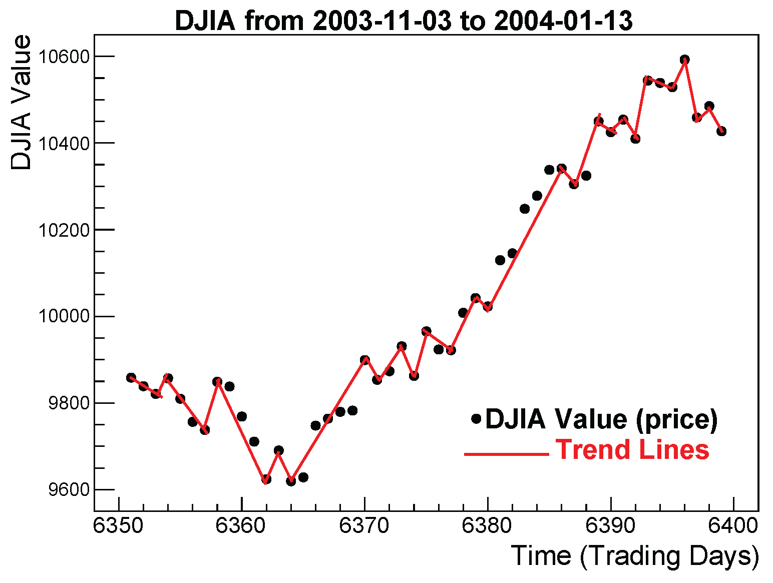
Figure 2.
Log-vertical distributions of uninterrupted trends duration in days for the 2(a) DJIA and 2(b) DJIA and Figure 2 IPC. Exponential model (red lines) fits very well both curves.
Figure 2.
Log-vertical distributions of uninterrupted trends duration in days for the 2(a) DJIA and 2(b) DJIA and Figure 2 IPC. Exponential model (red lines) fits very well both curves.
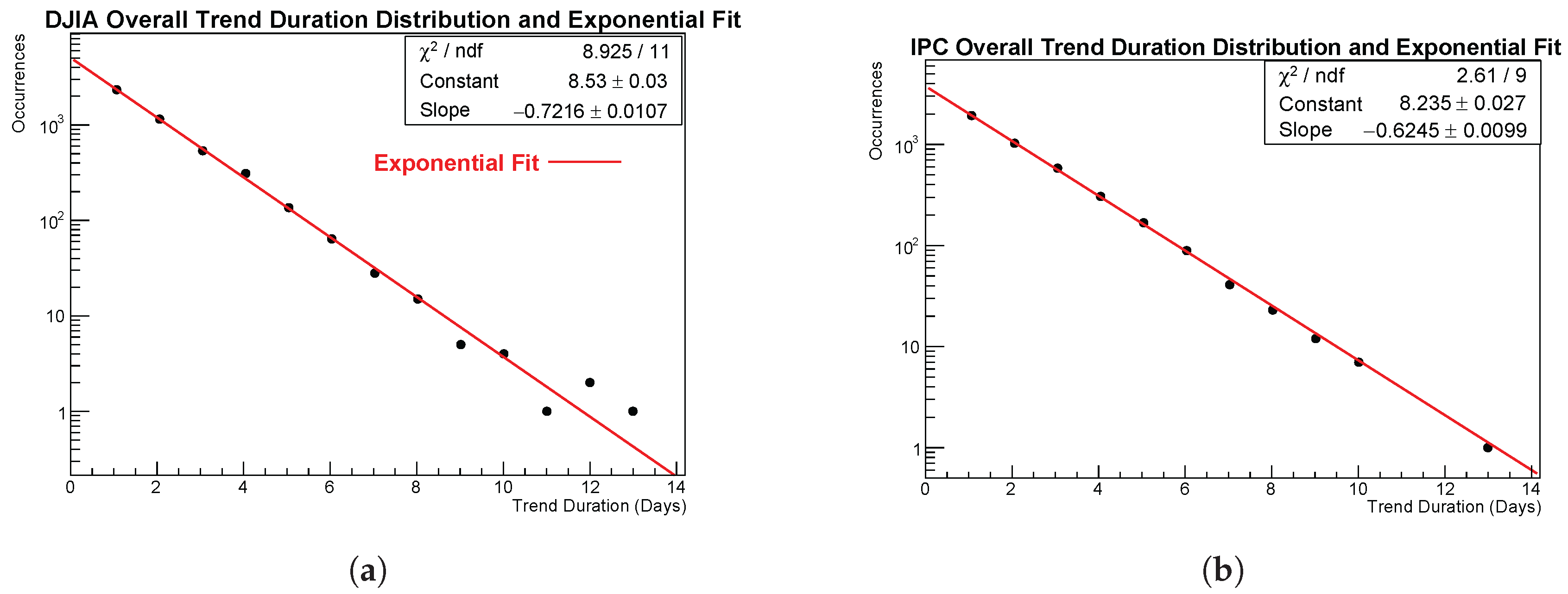
Figure 3.
Log-vertical distributions of uninterrupted trends duration in days for the following financial markets 3(a) DJIA downtrends, 3(b) DJIA uptrends, 3(c) IPC downtrends and 3(d) IPC uptrends, Figure 3 IPC downtrends and Figure 3 IPC uptrends. Again, exponential model (red line) fits very well the data.
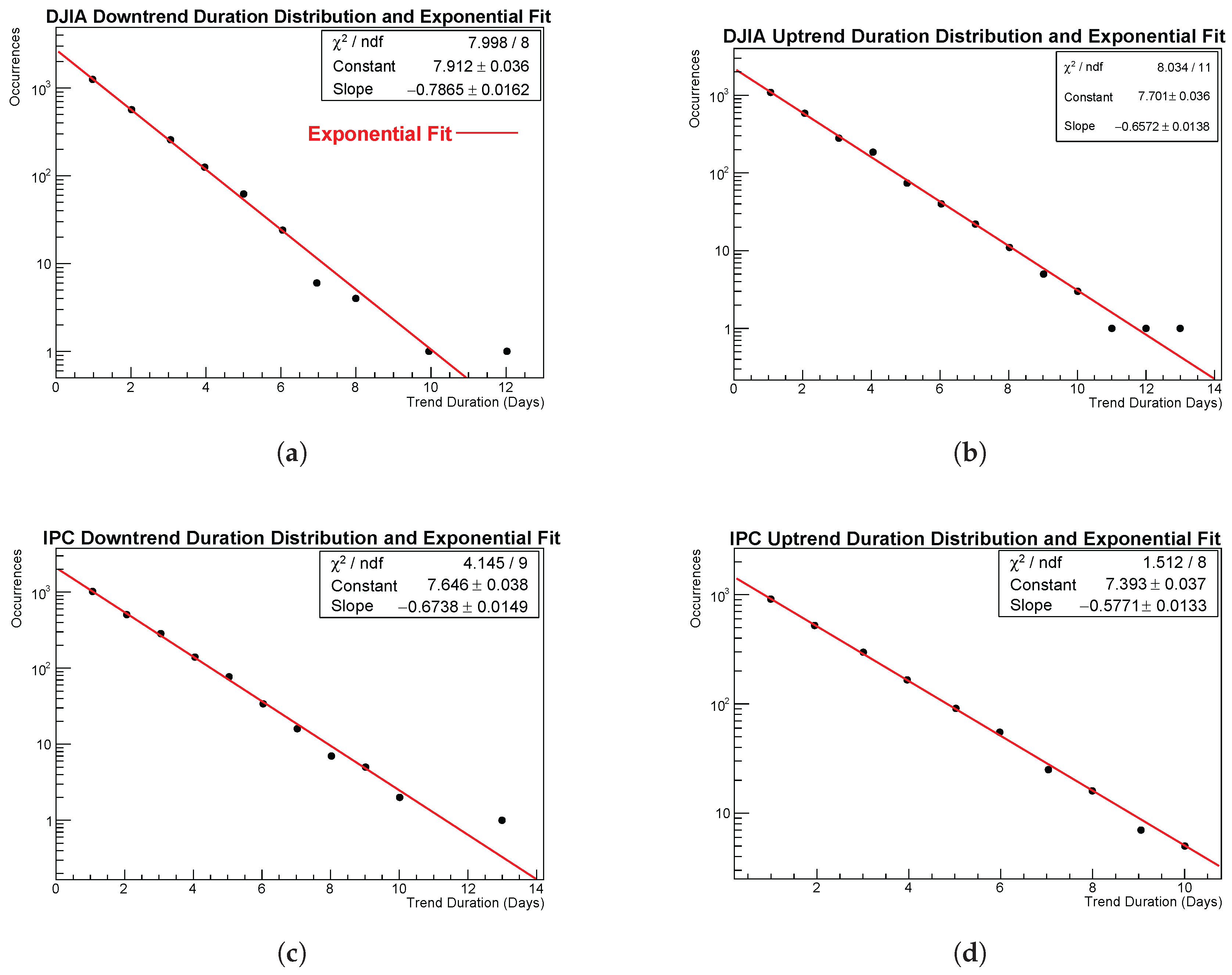
Figure 4.
Usual daily log-returns and TReturns evolution (darker line) for: DJIA 4(a) DJIA 4(c) IPC datasets. Panels 4(b) DJIA and 4(d) IPC display and compare the distributions of both distributions: Multi-Scale Returns (darker line) and usual daily log-returns (red line).
Figure 4.
Usual daily log-returns and TReturns evolution (darker line) for: DJIA 4(a) DJIA 4(c) IPC datasets. Panels 4(b) DJIA and 4(d) IPC display and compare the distributions of both distributions: Multi-Scale Returns (darker line) and usual daily log-returns (red line).
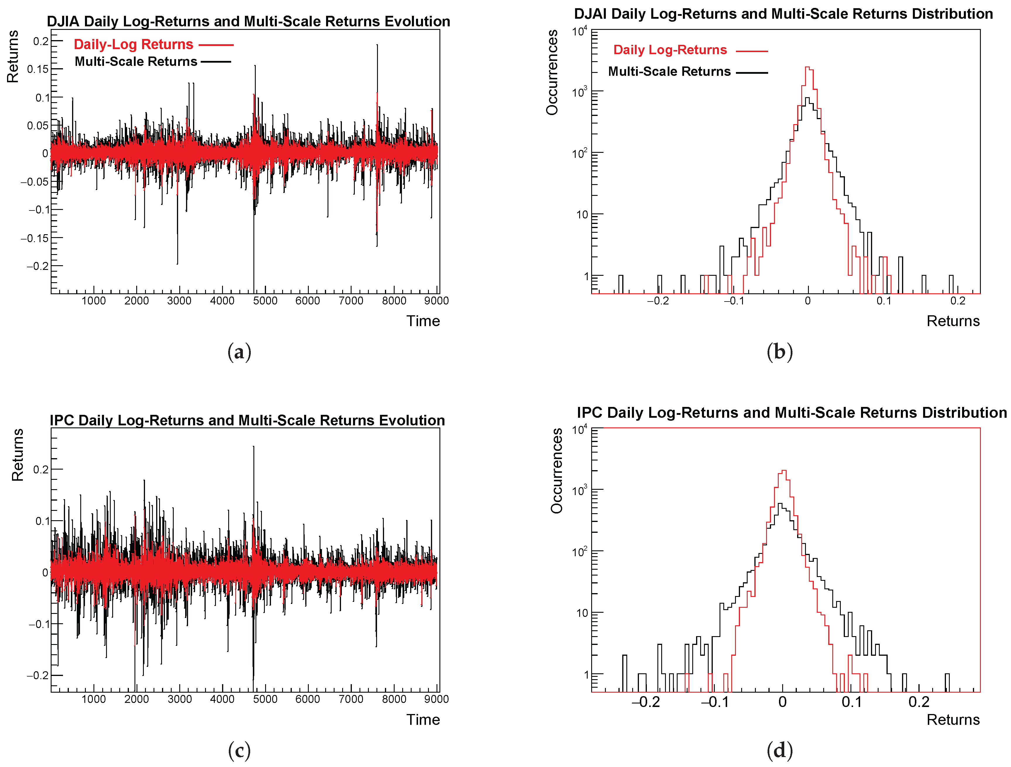
Figure 5.
TReturns positive and negative regions (-TReturns) in a log-vertical scale. Red lines correspond to exponential fits. Panel 5(a) shows -TReturns distribution for the negative region . Panel 5(b) shows the distribution of DJIA TReturns for the positive region, . Panel 5(c) shows the TReturns Distribution of IPC for the negative region and panel 5(d) shows IPC TReturns distribution for the positive region . All exponential fits accurately describe the four datasets in the described regions.
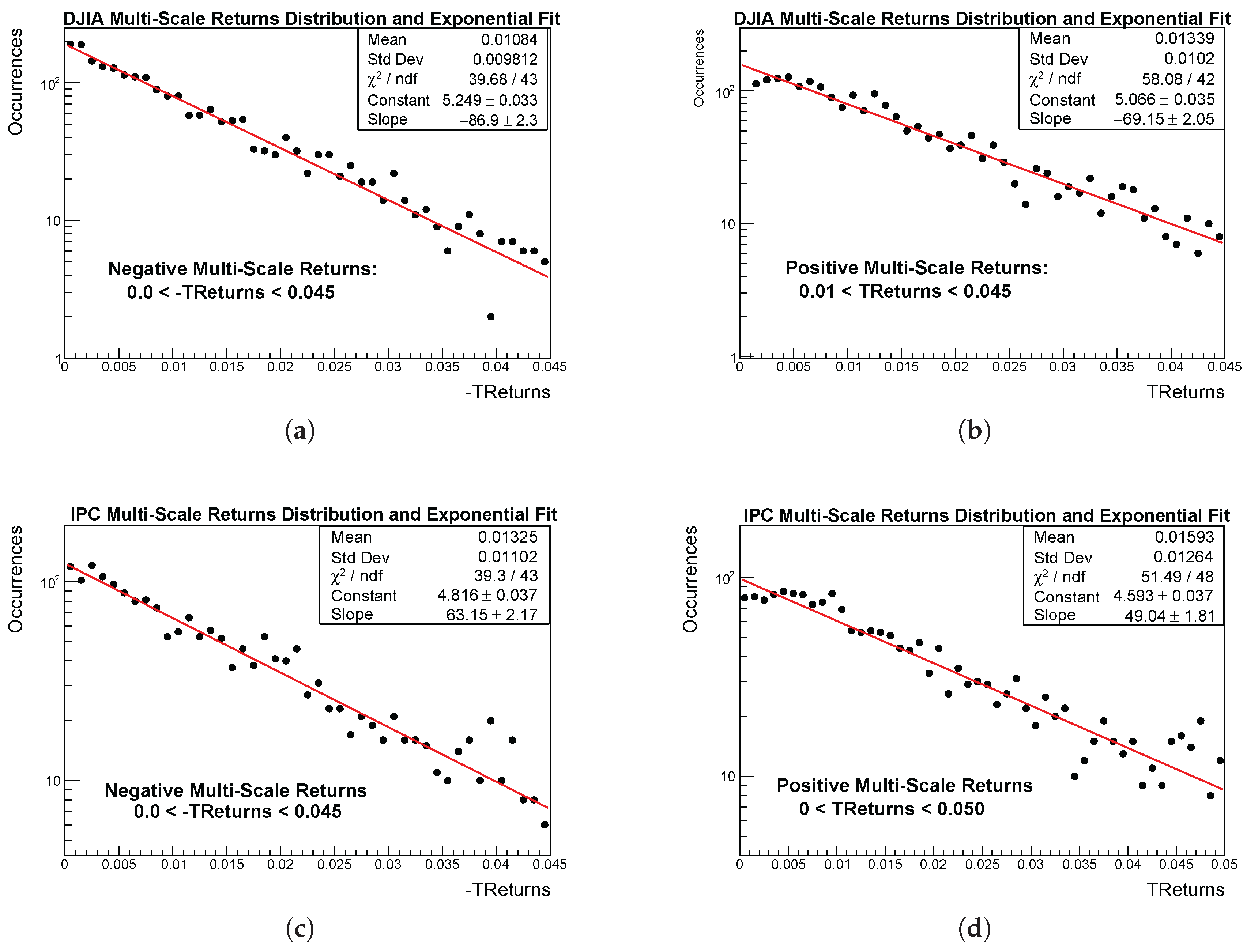
Figure 6.
TReturns distributions and corresponding power law fits (red lines) performed in negative (-TReturns>0) and positive (TReturns>0) asyntotic returns regions and usual daily log-returns: 6(a) left and 6(b) right asyntotic tails for DJIA negative and positive TReturns respectively; left 6(e), negative and right 6(f), positive tails for DJIA daily usual log-returns. Left 6(c), negative and right 6(d), positive asyntotic tails for IPC TReturns distribution; left 6(g) negative and right 6(h) positive tails for IPC daily log-returns distributions. Fitted regions are also pointed out graphically and numerically in all plots. Power law model fits correctly those asyntotic regions for the two kind of returns.
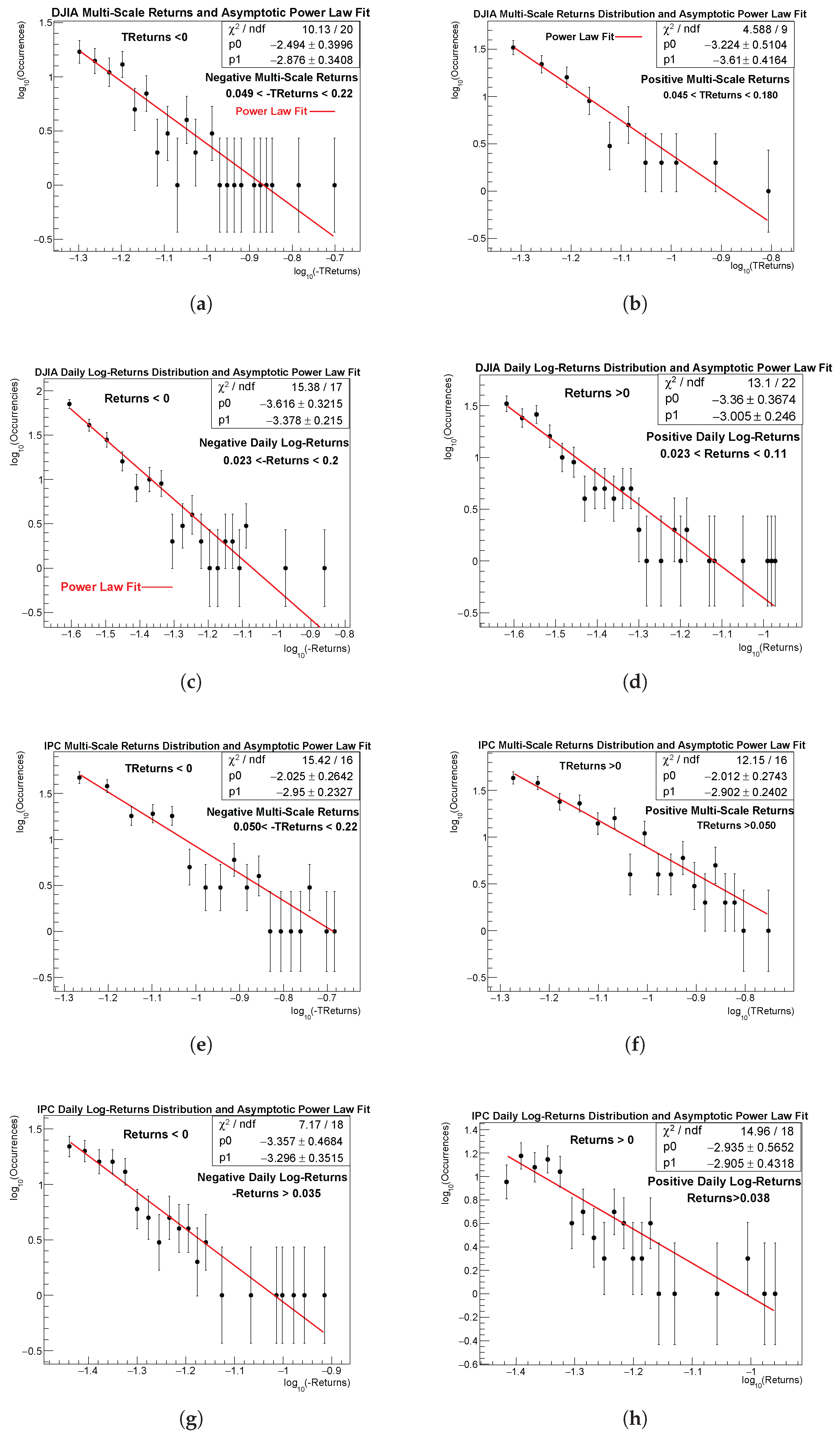
Table 1.
Descriptive statistics of run durations for DJIA and IPC, combining both uptrends and downtrends.
Table 1.
Descriptive statistics of run durations for DJIA and IPC, combining both uptrends and downtrends.
| Index | Daily records | Runs | Uptrends | Downtrends | Mean | Std Dev | Skewness | Kurtosis |
|---|---|---|---|---|---|---|---|---|
| DJIA | 9011 | 4595 | 2297 | 2298 | 2.020 | 1.352 | 2.077 | 6.251 |
| IPC | 8996 | 4189 | 2095 | 2094 | 2.147 | 1.513 | 1.887 | 4.155 |
Table 2.
Exponential fit parameters for overall (combined) trend durations.
| Index | Constant a | Slope b | Notes | |
|---|---|---|---|---|
| DJIA | - | all trends | ||
| IPC | - | all trends |
Table 3.
Run statistics for uptrends and downtrends.
| Market | Trend | Entries | Mean | Std Dev | Skew | Kur |
|---|---|---|---|---|---|---|
| DJIA | Downtrends | 2298 | 1.830 | 1.206 | 1.993 | 5.800 |
| Uptrends | 2297 | 2.091 | 1.487 | 2.103 | 5.859 | |
| IPC | Downtrends | 2094 | 2.045 | 1.424 | 2.014 | 5.291 |
| Uptrends | 2095 | 2.249 | 1.591 | 1.689 | 3.209 |
Table 4.
Exponential fits parameters for uptrends and downtrends.
| Market | Trend | Constant a | Slope b | |
|---|---|---|---|---|
| DJIA | Downtrends | 7.998/8 | ||
| Uptrends | 8.034/11 | |||
| IPC | Downtrends | 4.145/9 | ||
| Uptrends | 1.512/8 |
Table 5.
Descriptive statistics for DJIA and IPC daily and multi-scale returns (January/02/1990–October/17/2025).
Table 5.
Descriptive statistics for DJIA and IPC daily and multi-scale returns (January/02/1990–October/17/2025).
| Dataset (Returns) | N | Mean | Std | Min | Max | Skewness | Kurtosis |
|---|---|---|---|---|---|---|---|
| DJIA Multi-Scale R | 4596 | 0.0006 | 0.0217 | 0.1931 | 12.08 | ||
| DJIA Daily R | 9010 | 0.0003 | 0.0109 | 0.1076 | 12.64 | ||
| IPC Multi-Scale R | 4191 | 0.0012 | 0.0315 | 0.2442 | 7.22 | ||
| IPC Daily R | 8995 | 0.0006 | 0.0138 | 0.1215 | 6.67 |
Table 6.
Exponential fit parameters for low and medium positive and negative TReturns distribution. The constant parameter a is omitted as it plays no role in interpreting the exponential decay rates; only the slopes are reported.
Table 6.
Exponential fit parameters for low and medium positive and negative TReturns distribution. The constant parameter a is omitted as it plays no role in interpreting the exponential decay rates; only the slopes are reported.
| Market TRets | Region | Region | ||||
|---|---|---|---|---|---|---|
| DJIA TRets | -86.90 ± 2.30 | -0.045<TRets<0 | 36.68/43 | -69.15 ± 2.05 | 0.01<TRets<0.045 | 58.08/42 |
| IPC TRets | -63.15 ± 2.17 | -0.045<Rets<0 | 39.3/43 | -49.04 ± 1.81 | 109.7/90 |
Table 7.
Asymptotic power-law fits for multi-scale returns (TReturns) and usual daily log-returns for the DJIA and IPC. Fits correspond to the log-log PDF representations shown in Figure 6. In this table, for reasons of space, R denotes simple daily log-returns and denotes the trend returns. The PDF tail exponent is .
| Market | Returns Type | Tail | Fit Range | ||||
|---|---|---|---|---|---|---|---|
| DJIA | TReturns | Negative | |||||
| Positive | |||||||
| DJIA | Daily log-returns | Negative | |||||
| Positive | |||||||
| IPC | TReturns | Negative | |||||
| Positive | |||||||
| IPC | Daily log-returns | Negative | |||||
| Positive |
Table 10.
File sizes (in kilobytes) for daily returns and TReturns before and after ZIP compression, together with the percentage of the original size that remains after compression.
Table 10.
File sizes (in kilobytes) for daily returns and TReturns before and after ZIP compression, together with the percentage of the original size that remains after compression.
| Dataset | Plain Text (kB) | ZIP (kB) | Compression (%) |
|---|---|---|---|
| DJIA daily returns | 99 | 36 | 36% |
| DJIA TReturns | 50 | 19 | 38% |
| IPC daily returns | 98 | 36 | 37% |
| IPC TReturns | 45 | 17 | 38% |
Disclaimer/Publisher’s Note: The statements, opinions and data contained in all publications are solely those of the individual author(s) and contributor(s) and not of MDPI and/or the editor(s). MDPI and/or the editor(s) disclaim responsibility for any injury to people or property resulting from any ideas, methods, instructions or products referred to in the content. |
© 2025 by the authors. Licensee MDPI, Basel, Switzerland. This article is an open access article distributed under the terms and conditions of the Creative Commons Attribution (CC BY) license (http://creativecommons.org/licenses/by/4.0/).
Copyright: This open access article is published under a Creative Commons CC BY 4.0 license, which permit the free download, distribution, and reuse, provided that the author and preprint are cited in any reuse.


