
Submitted:
12 December 2024
Posted:
12 December 2024
You are already at the latest version
Abstract
We propose a test statistic that is useful to identify that increments in high-frequency time series data of prices follow a jump-diffusion model. The main result and contribution of this study shows that the distribution function of our proposed test statistic follows approximately a gamma distribution. This result is crucial because it enables us to determine the critical region for the rejection of the null hypothesis of interest. We show that the detection power and error rate of our proposed test statistic is better than a test statistic used as benchmark, showing a higher detection power and lower error rate. We applied our proposed test using high-frequency transaction prices of Google, Apple and Goldman Sachs stocks and found that our proposed test statistic captures the dynamics of the series.
Keywords:
jumps
; quantile
; semimartigales
; statistic
; test
; variation
1. Introduction
Historically, the volatility of financial time series has been treated in two ways. The first approach is parametric and postulates a latent variable via conditional heteroscedastic models to describe the volatility, such as the ARCH (Autoregressive Conditional Heterocedasticity) family models proposed by [10] and the stochastic volatility models, proposed by [18]. There is a huge literature on this approach and for details, see, for example, [17,21].
The main motivation for using the nonparametric approach is because parametric models often fail to adequately capture the movements of intraday volatility, see [1]. A nonparametric approach consists of constructing the daily realized volatility (RV) of a financial series using intraday returns, sampled at intervals , of the order of 5 or 15 minutes, for example. RV is obtained from sums of squares of intraday returns, see [1] and [6]. Another method is to construct the realized bi-power variance (RVBP), from the sums of cross products of absolute adjacent, properly scaled returns, see [7]. For details, see [5]. [7,12] and [2] derived test statistics for detecting the existence of jumps. Other authors established tests for the necessity of adding a Brownian force, see [3,14,16,20] and [19]. [4] studied whether the jump component is of finite activity when the Brownian force is present.
In recent years, efforts have been devoted to study the distribution function of test statistics in the presence of jumps. [15] studied whether it is necessary to add an infinite variation jump term in addition to a continuous local martingale, using a Kolmogorov-Smirnov (KS) type test statistic. [8] derived the exact and asymptotic distribution of Cramér-von mises statistic when the empirical distribution function is a uniform distribution function. [20] suggested using other measures of discrepancy between distributions, as the Cramér-von mises test for the presence of diffusion component in a process which usually represents the price (or log-prices) of some financial asset. These studies motivated us to propose a test statistic using a Cramér-Von Mises type statistic.
It would be important to obtain the distribution of our proposed test statistic in the presence of jumps, however this is not an easy task, so we will employ numerical methods to approximate this distribution.
The paper is organized as follows. In Section 2 we establish the set up for our problem, define the hypotheses of interest and discuss the choice of the proposed test statistic. Section 3 discuss an approximation to the true distribution of the statistics, whereas Section 4 presents a simulation study to assess its performance. Section 5 applies our proposed test statistic to real data and Section 6 concludes with comments on the usefulness of the proposed methodology and on recommendations for future works.
2. Setup
The standard jump-diffusion model used for modeling many stochastic processes is given by the following differential equation:
where and are processes with càdlàg paths, is a standard Brownian motion, and is an Itô semimartingale process of pure-jump type. [20] generalized Eq. (1) to accommodate the alternative hypothesis that can be of pure-jump type. Itô semimartingale plays an important role in stochastic calculus and the following model plays a major role.
Suppose that follows a non-parametric volatility model
where is a continuous Itô semimartingale, that is,
where is the drift term with being an optional and càdlàg process, is a continuous local martingale with being an adapted process, is a standard Brownian motion, and is a skewed -stable Lévy process.
[15] provided a theoretical test for the presence of infinite variation jumps in the simultaneous presence of a diffusion term and a jump component of finite variation and established the asymptotic theory of the empirical distribution of the “devolatilized" increments of Itô semimartingale with infinitely active or even infinite variation jumps. There are other methods to estimate the spot volatility, see, for instance, [20] and [11].
Recently, [9] discussed a volatility functional model and showed that jumps asymptotically impact the volatility estimate and presented a jump detection model based on wavelets.
We now consider the following hypotheses
where denotes the ith one-step increment for and we assume that the available data set are discretely equally spaced variables sampled from , in the fixed interval , i.e., with for . The empirical process is given by:
for a finite sample size n, and are some integer depending on n, should be smaller than , should be smaller than and denotes the integer part. Here, denotes the distribution function (df) of a standard normal random variable and is the empirical distribution function (edf) of the devolatilized increments. We used the local estimator proposed by [20] to estimate . On each of the blocks the local estimator of is given by
which is the bipower variation for measuring the quadratic variation of the diffusion component of . [20] removed the high-frequency increments that contain big jumps. The total number of increments used in their statistic is thus given by
where and . They use a time-varying threshold in the truncation to account for the time varying . The scaling of every high-frequency increment is done after adjusting to exclude the contribution of that increment in its formation:
Then, they define
which is simply the edf of the devolatilized increments that do not contain any big jumps. In the jump-diffusion case of Eq. (1), should be approximately the df of a standard normal random variable. [20] use an alternative estimator of the volatility that is the truncated variation defined as
where and, the corresponding one excluding the contribution of the ith increment for , is
The edf of the devolatilized (and truncated) increments is given by,
where . Here, the total number of increments is defined as
We define the test statistic as:
where A is a compact set in and . Here, is an edf and we assume that is the df of a standard normal random variable and use the notation for it. So, we have
The critical region for the test is given by
where A is a compact set in and is the -quantile of the distribution of the statistic. We evaluate via simulation. The test rejects if . The main purpose is to develop a test statistic that has better statistical properties than the existing KS test statistic for identifying jump variations in high-frequency time series. We will use the notation and for when using Eqs. (6) and (9), respectively. To determine the critical region of the test we will perform extensive simulations, using the R language, version . All data and codes are available upon request to the authors.
2.1. Performance of Test Statistics
The idea is to observe which test statistic performs better using the two df mentioned in the previous section. A simulation was performed with replications and different n, and values, as shown in the following panel.
| n | |
| , , , , , , , , | |
| , , , , , | |
| , , , , , , , | |
| , , , , , , | |
| , , , , , | |
| , , , , , , , | |
| , , , , , , , | |
| , , , , , , | |
| , , , , , , | |
| , , , , . |
Figure 1 shows the behavior of and test statistics against , for the jump-diffusion model. From the plots, we observe the existence of outliers. Also, the values of and test statistics increase as increases. In cases where and , the values of the test statistics present some inconsistencies.
Figure 2 shows the behavior of and test statistics against , for the standard normal model.
The first simulations were based on replicas with and the same pairs of and as mentioned above. The mean squared distance (MSD) is the difference between the values observed of test statistics from the two models used. It can be observed in Figure 3 that, for the jump-diffusion model, the MSD of test statistic increases as increases. On the other hand, for the normal model, on the average, the MSD of test statistics stabilizes, that is, the values of test statistics are close as increases.
One purpose is to estimate the best critical value of test statistics to choose which test performs better.
The ROC (Receiver Operating Characteristic) curve is widely used to determine the cutoff point. The best critical value is obtained using simulation. A ROC curve can be described as the shape of the trade-off between the sensitivity and the specificity of a test, for every possible decision rule cutoff (or threshold) between 0 and 1. The optimal cutoff point is the one closer to the point, and this gives the values of the specificity and sensitivity of the test. The area under the ROC curve (AUC) gives the accuracy of the test. The larger the area, the larger the accuracy of the test. In our case, we will call the sensitivity by detection power and 1-specificity the error rate.
2.2. The Best Critical Value
We test the critical value q between 1 and 3, and used the ROC curve to find the cutoff point. We compare the detection power and error rate for these values and a fixed critical value. Table 1 shows that, for test statistic with a fixed critical value , the error rate for is around and the detection power is . In contrast, for test statistic, the error rate is around and the detection power is . It can also be seen that, for low values of , there are low error rates but with low detection power. For example, for , with , there is an error rate around and a detection power of and, for , we observe of error rate and of detection power. Moreover, for the optimal critical value , with , we have an error rate of and a detection power of for and, for , an error rate of and of detection power.
Figure 4 shows the detection power and error rate for a fixed critical value .
Figure 5 shows the detection power and error rate of a simulated critical value , that were obtained through the respective ROC curves in Figure 6. We repeat our simulation for and the same pairs of and already mentioned above. The conclusion is similar to .
The MSD of test statistics, are shown in Figure 7.
Figure 8 shows the detection power and error rate for a fixed critical value .
Table 2 shows the detection powers and error rates for two critical values, a fixed and simulated, which lead us to conclude that test statistic is better than test statistic. For example, for with , we have an error rate of and a detection power of for test statistic whereas test statistic presents an error rate of and a low detection power of .
Figure 9 shows the detection power and error rate for , obtained by simulation, with the ROC curves in Figure 10. It can be seen that as increases the error rate for is higher than and, for the detection power, as increases, has a higher detection power than . Again, test statistic seems to be better than test statistic.
We can observe in Figure 11 that the MSD of the test statistics has a similar behavior to the previous analysis.
We are interested in the largest squared distance, so the pairs of for , we will be used for our study for the aforementioned reasons.
Figure 12 shows the detection power and error rate for a fixed critical value .
Figure 13 shows the detection power and error rate considering a simulated critical value, obtained by ROC curve, see Figure 14.
Table 3 shows that, for a fixed value , the error rate for test statistic, with is around and the detection power is . In contrast, for the test statistic , the error rate is around and detection power of . It can also be seen that, for low values for test statistic, there are low error rates but with low detection power. For example, taking , for test statistic, there is an error rate around and of detection power. On the other hand, for the simulated critical value obtained by ROC curve and , we have an error rate of and a detection power of for test statistic and for , we observe an error rate of and a detection power of .
Remark: Note that; Table 1, Table 2 and Table 3 for and values, the error rate and detection power show inconsistent values, due to a high false alarm rate and not so much detection power. Therefore, we do not recommend using low values of .
We will use test statistic, since it presented better results in relation to low error rate and high detection power. The ideal is to choose a that shows a low error rate and high detection power.
In contrast, for test statistic, there is high error rate and low detection power for most values. See also Table 4. Also, the area under the ROC curve of shows a larger area, and therefore the larger the area, the greater the accuracy of the test, which leads us to conclude that our test is better than .
3. Aproximating the edf of TA2
As we remarked before, the purpose would be to derive the df of . However, this is very hard theoretically and therefore we will address the problem using numerical methods. Our simulation shows that the edf of test statistic is approximately a gamma distribution, with values in the good agreement, see Figure 15.
Figure 16 shows that we have a very good approximation with the true density. For the gamma density with parameters a and b, given that and , its df is , which can be written as , where is the incomplete gamma function. For large sample sizes (see Table 5), we have and , so we can write, approximately, , with and Var.
In Table 6 we can find the quantiles of gamma and empirical distribution for different probabilities. Note that the theoretical quantiles compared with the empirical quantile are closer for probabilities higher than .
4. A simulation Study
We conduct a simulation study to check the performance of the test statistic. Figure 17 shows data generated from the jump-diffusion and standard normal models that we used in our study.
The models are defined as follows: the jump-diffusion model is given by,
where is a skewed Lévy process. The volatility is a square root diffusion process which is widely used in financial applications. The parameter in is specified as in [13]. The standard normal model is , where is the initial value that should be defined.
We considered replicas for sample sizes and . For the truncation of the increments, as is typical in the literature, we set and . Hence for the sampling frequencies mentioned in Section 2, we set the pairs of as: , , , and with ranging from to and having an increasing trend.
In Table 7 we can observe that the test power increases as the sample size increases and also, for n fixed, test power is bigger for largest values. The test power was calculated with the gamma quantile values, and we note that these values are very close to the empirical quantiles. To evaluate the performance of our test, we compare with the KS test, which also measures discrepancy between distributions.
In Table 8 we note that the test statistic shows better results. Moreover, the KS test power decreases and the error rate increases as n increases. For , KS test power is bigger than test power, however test statistic has an error rate of and KS test has an error rate bigger than . For larger sample sizes, the test statistic shows better test power with low error rate. Besides, KS test power decreases and the error rate increases as n increases. For , KS test power is bigger than test power, however test statistic has an error rate of and KS test has an error rate bigger than .
For larger sample sizes, the test statistic shows better power with low error rate.
5. Real Data Analysis
We collect intraday transaction prices of the Apple, Google and Goldman Sachs (GS) stocks, respectively, from November 11th to November 12th in 2014, with a sampling frequency of 15 seconds. The transaction records that are outside the ranges of quotes, 9:30 a.m to 4:00 p.m, are excluded. There are, in total ; and stock of prices, respectively. We aim to plot the observed test statistics against different values of and . Figure 18 shows the price series for market data of Apple, Google and GS stocks.
Figure 19 shows the values of the test statistic, for different values.
Additionally, we illustrate the quantile values at the significance level of and . The plots (a), (c) and (e) of Figure 19 consider the values of between , and for the three stocks considered, respectively. The plots (b), (d) and (f) of Figure 19 show values starting from 44, that is, we show an enlarged version of the plots (a), (c) and (e) of Figure 19. It can be seen in Table 9 that, at a level of significance of , Apple stock rejects null hypothesis, whereas Google and GS stocks do not.
On the other hand, when we increase the level of significance to , the percentage increases for all stocks, with Apple still rejecting , while Google and GS do not. Here we have used all values. For sufficiently large values of , our test statistic tends to detect more precisely the dynamics of the Apple and GS series as can be seen in Table 10.
6. Conclusions
In this paper we discussed the approximate distribution of the proposed test statistic when the empirical distribution function is approximated by a gamma distribution function. This result is important, because it enables us to determine the critical region for the null hypothesis. Also, the real data analysis shows that our proposed test statistic is useful to identify that increments in time series like Apple and GS stocks, follow a jump-diffusion model for high-frequency data of prices for the largest values. Market activity on a trading day records containing a lot of price information between transactions is very important because it allows us to know the behavior of the micro-structure of market prices.
As a future work, we can explore the behavior of our proposed test statistic considering other financial time series, for different time records between transactions, i.e., with a sampling rates of 1, 2 or 5 seconds. In finance and econometrics it is still an open problem, being able to anticipate and/or measure a threshold, i.e., the size of the big losses that will occur on some day of trading on the stock exchange, or of big gains, given the need to mitigate the risk of any portfolio in question. Finally, another challenge for future research is to find the exact distribution of the test statistic.
Funding
This research was funded by a fellowship to William Rojas Duran by the International Cooperation Program CAPES/PDSE of Brazil grant 88881.131503/2016-01, at the Booth School of Business, University of Chicago.
Acknowledgments
I thank the University of São Paulo, Brazil, for all the support during my Ph.D. Also to my mother, Lucila Duran, my main support, motivation and inspiration.
Conflicts of Interest
The authors declare no conflicts of interest.
References
- Andersen, T. G., Bollerslev, T., Diebold, F. X and Labys, P. Modeling and forecasting realized volatility. Econometrica 2003, 10, 579–625. [CrossRef]
- Aït-Sahalia, Y and Jacod, J. Testing for jumps in discretely observed process. Ann. Stat, 2009, 37, 184–222. [CrossRef]
- Aït-Sahalia, Y and Jacod, J. Is Brownian motion necessary to model high-frequency data?. Ann. Stat, 2010, 38, 3093–3128. [CrossRef]
- Aït-Sahalia, Y and Jacod, J. Testing whether jumps have finite or infinite activity. Ann. Stat, 2011 39, 1689–1719. [CrossRef]
- Aït-Sahalia, Y and Jacod, J. High-frequency financial econometric. Princeton University Press, 2014.
- Barndorff-Nielsen, O. E. and Shephard, N. Econometric analysis of realized volatility and its use in estimating stochastic volatility models. Journal of the Royal Statistical Society Series B, 2002, 64, 253–280. [CrossRef]
- Barndorff-Nielsen, O. E. and Shephard, N. Econometrics of testing for jumps in financial economics using bipower variation. Journal Finacial Econometrics, 2006, 2, 1–48. [CrossRef]
- Csorgo, S. and Faraway, J. The Exact and Asymptotic Distributions of Cramér-von Mises Statistics. J. R. Statist. Soc. Series B, 1996, 58, 221–234. [CrossRef]
- Duran, W. R. and Morettin, P. A. Identifying jumps in high-frequency time series by wavelets. International Journal of Wavelets, Multiresolution and Information Processing, 2024. [CrossRef]
- Engle, R.F. Autoregressive conditional heteroscedasticity with estimates of the variance of United Kingdom inflation. Econometrica 1982, 50, 987–1008. [Google Scholar] [CrossRef]
- Fan, J. and Wang, Y. Multi-scale jump and volatility analysis for high-frequency financial data. Journal of the American Statistical Association, 2007, 102, 1349–1362. [CrossRef]
- Fan, J. and Wang, Y. Spot volatility estimation for high-frequency data. Stat. Interf, 2008, 1, 279–288. [CrossRef]
- Jacod, J. and Todorov, V. Efficient estimation of integrated volatility in presence of infinite variation jumps. Ann. Stat., 2014, 42(3), 1029–1069. [CrossRef]
- Jing, B. Y., Kong, X. B. and Liu, Z. Modeling high-frequency financial data by pure jump models. Ann. Stat, 2012, 40, 759–784. [CrossRef]
- Kong, X. B. Lack of Fit Test for Infinite Variation Jumps at High Frequencies. Statistica Sinica, 2017. [CrossRef]
- Kong, X. B., Liu, Z. and Jing, B. Y. Testing for pure-jump processes for high-frequency data. Ann. Stat, 2015, 43, 847–877. [CrossRef]
- Morettin, P. A. Financial Econometrics, 3rd ed.; Blucher: São Paulo, Brazil, 2017.
- Taylor, S. J. Financial returns modelled by the product of two stochastic processes - A study of daily sugar prices 1961-1979. In Time Series Analysis: Theory and Practice 1; Anderson, O.D. Ed.; Amsterdam: North Holland, 1982; 203–226.
- Todorov, V. Jump activity estimation for pure-jump semimartingales via self-normalized statistics. Ann. Stat. 2015, 43, 1831–1864. [Google Scholar] [CrossRef]
- Todorov, V. and Tauchen, G. Limit theorems for the empirical distribution function of scaled increments of Ito semimartingales at high frequencies. Ann. Appl. Prob, 2014, 24, 1850–1888. [CrossRef]
- Tsay, R. S. Analysis of Financial Time Series, 3rd. ed.; Wiley: New Jersey, United States of America, 2010.
Figure 1.
Behavior of and test statistics against for the jump-diffusion model. The simulation were based on replicas and different n values. (a) . (b) . (c) . (d) . (e) . (f) .
Figure 1.
Behavior of and test statistics against for the jump-diffusion model. The simulation were based on replicas and different n values. (a) . (b) . (c) . (d) . (e) . (f) .
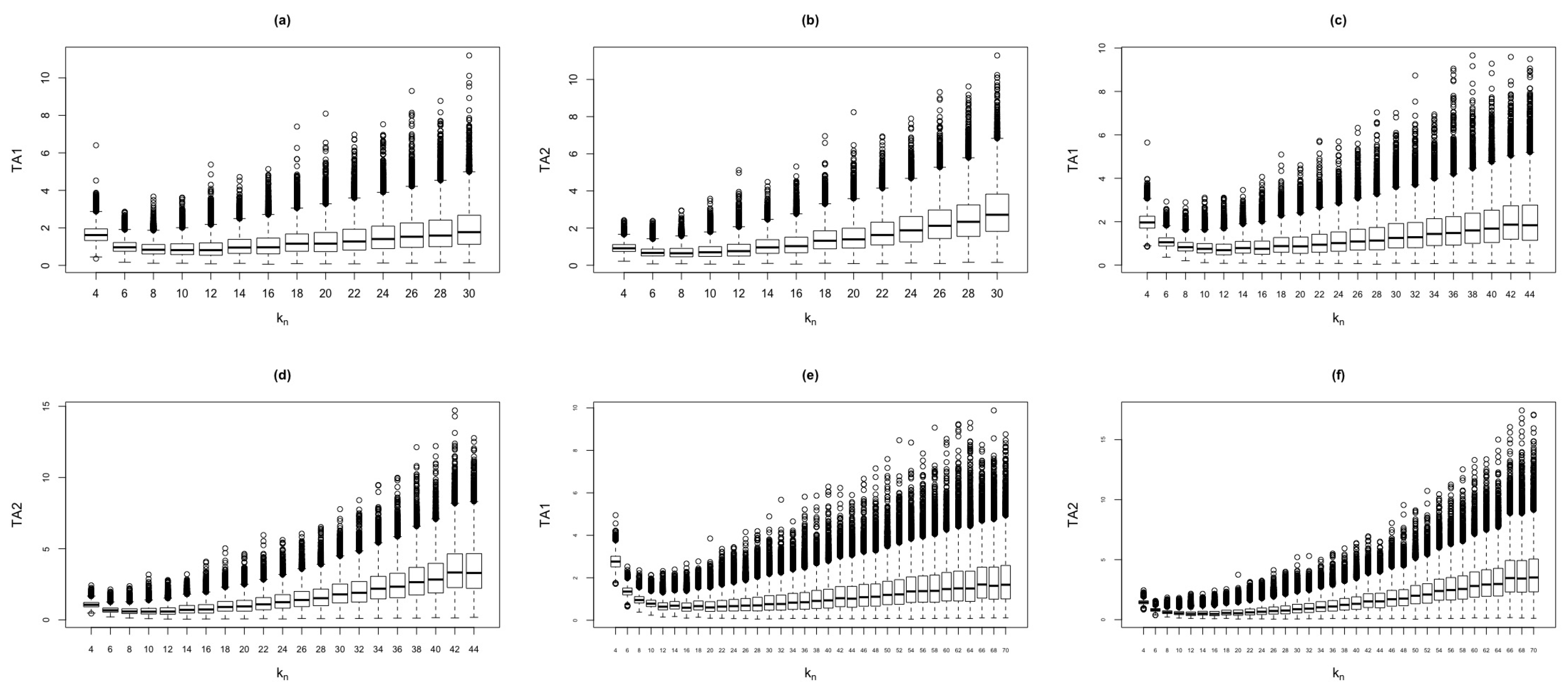
Figure 2.
Behavior of and test statistics against for the standard normal model. The simulation were based on replicas and different n values. (a) . (b) . (c) . (d) . (e) . (f) .
Figure 2.
Behavior of and test statistics against for the standard normal model. The simulation were based on replicas and different n values. (a) . (b) . (c) . (d) . (e) . (f) .
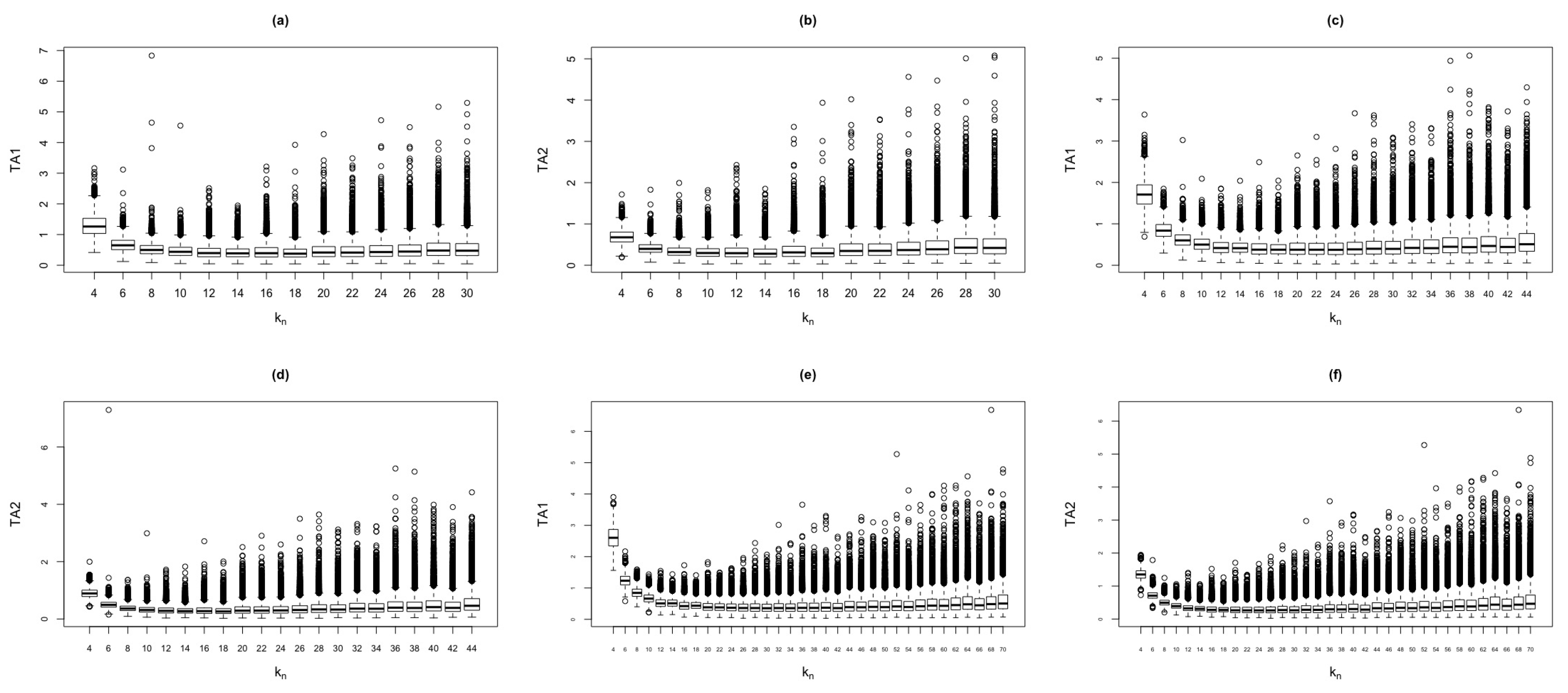
Figure 3.
MSD of test statistics for different values in data generated from the jump-diffusion (blue triangle) and standard normal (black circle) models with .
Figure 3.
MSD of test statistics for different values in data generated from the jump-diffusion (blue triangle) and standard normal (black circle) models with .
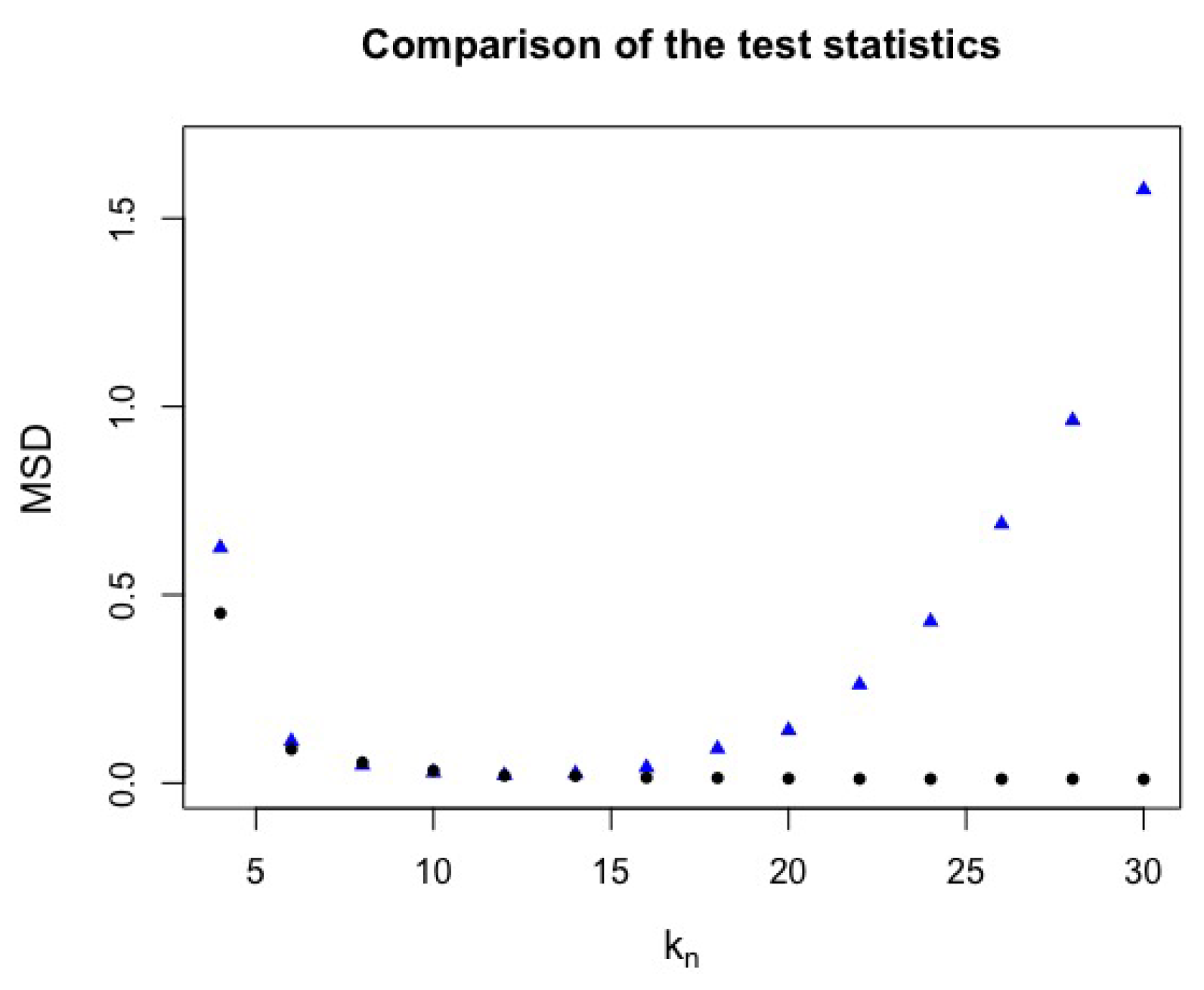
Figure 4.
Error rate and detection power with critical value and different values with . (a) Error rates for (black circle) and (blue triangle) test statistics. (b) Detection powers for (black circle) and (blue triangle) test statistics.
Figure 4.
Error rate and detection power with critical value and different values with . (a) Error rates for (black circle) and (blue triangle) test statistics. (b) Detection powers for (black circle) and (blue triangle) test statistics.
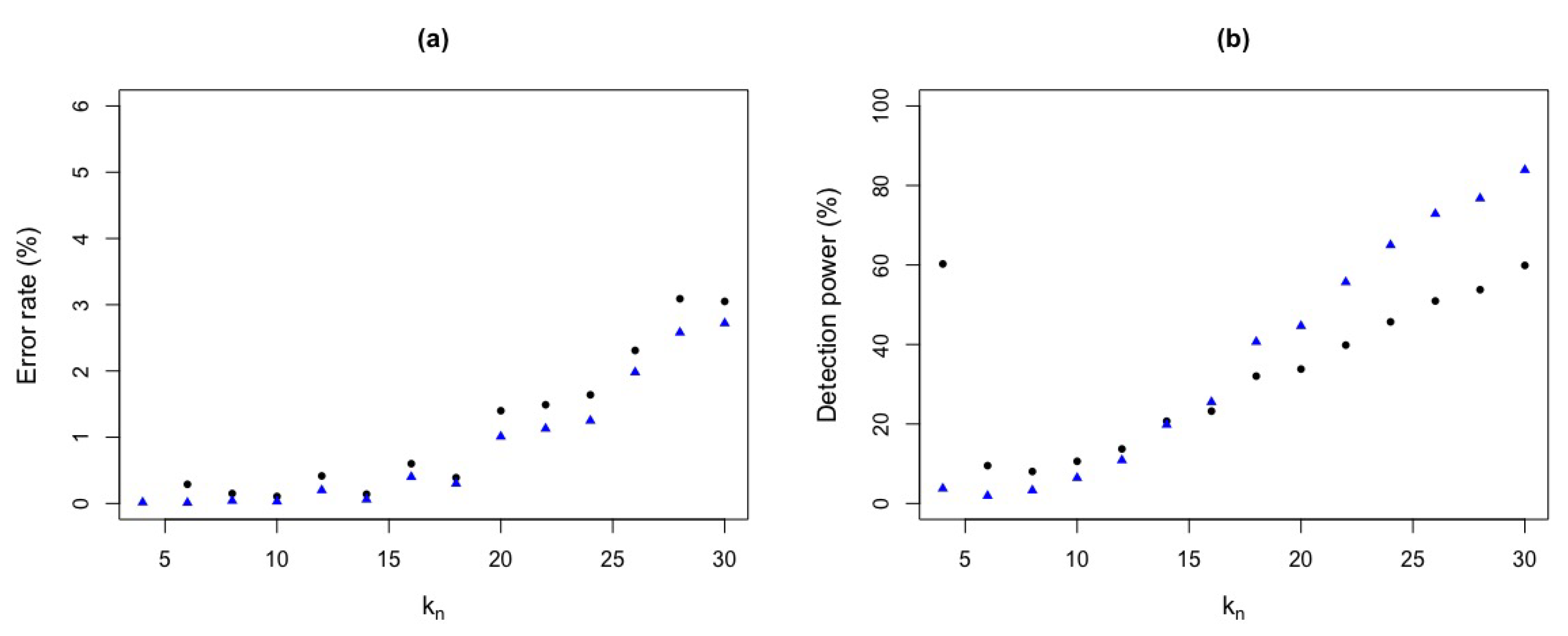
Figure 5.
Error rate and detection power with critical value and different values with . (a) Error rates for (black circle) and (blue triangle) test statistics. (b) Detection powers for (black circle) and (blue triangle) test statistics.
Figure 5.
Error rate and detection power with critical value and different values with . (a) Error rates for (black circle) and (blue triangle) test statistics. (b) Detection powers for (black circle) and (blue triangle) test statistics.
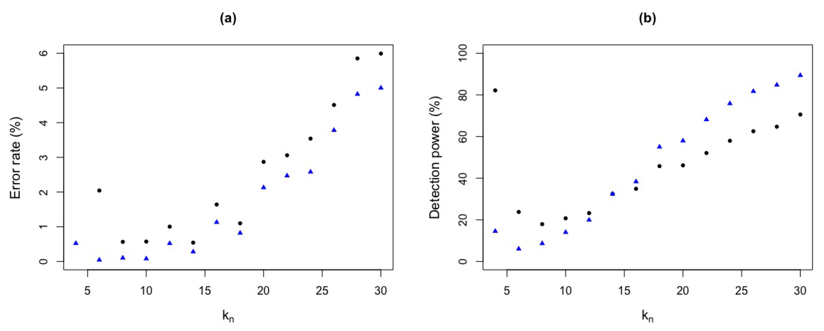
Figure 6.
ROC curve for and test statistics for Figure 5. (a) ROC curve . (b) ROC curve .
Figure 6.
ROC curve for and test statistics for Figure 5. (a) ROC curve . (b) ROC curve .
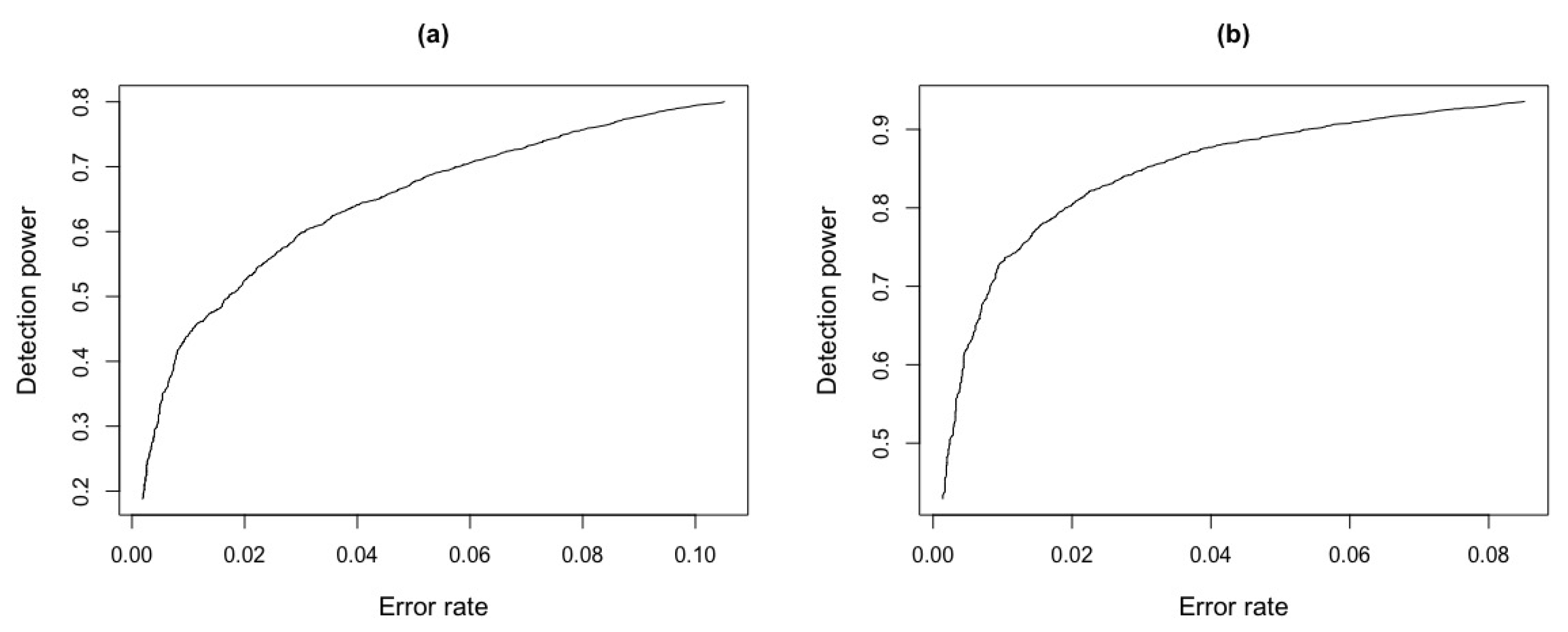
Figure 7.
MSD of test statistics for different values, in data generated from the jump-diffusion (blue triangle) and standard normal (black circle) models with .
Figure 7.
MSD of test statistics for different values, in data generated from the jump-diffusion (blue triangle) and standard normal (black circle) models with .
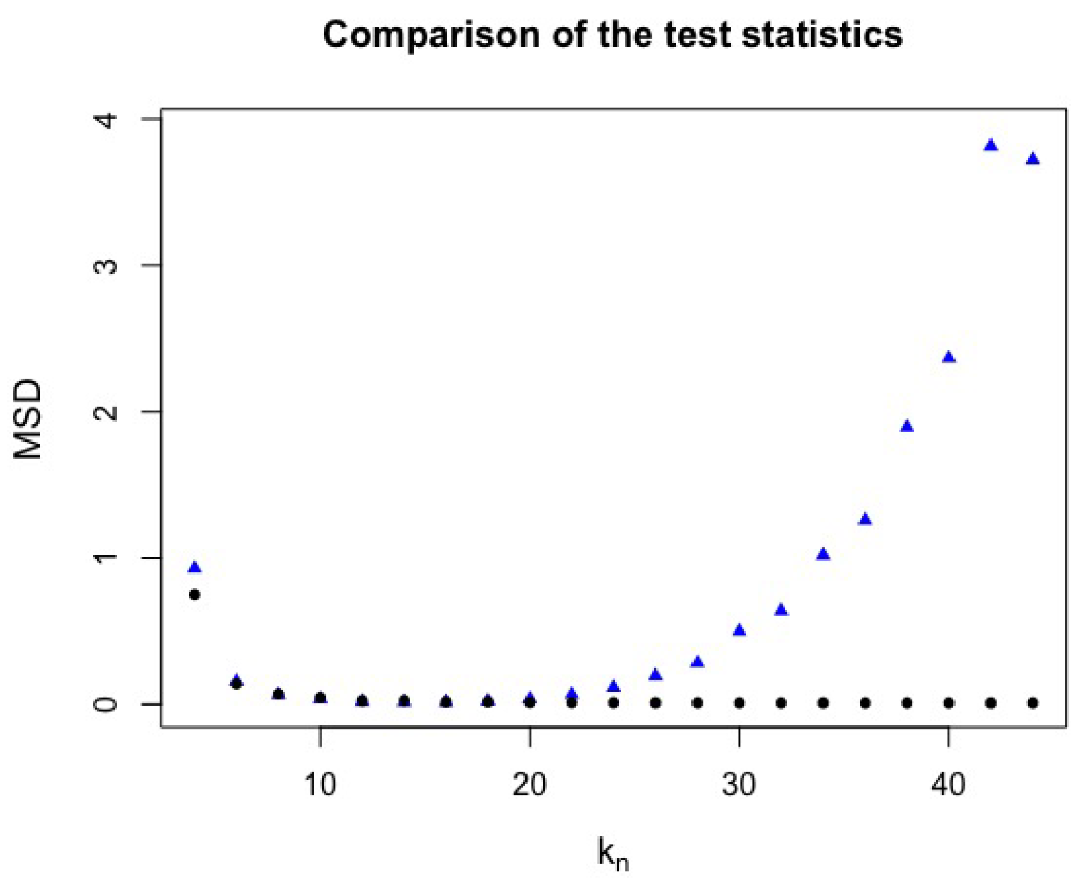
Figure 8.
Error rate and detection power with critical value and different values with . (a) Error rates for (black circle) and (blue triangle) test statistics. (b) Detection powers for (black circle) and (blue triangle) test statistics.
Figure 8.
Error rate and detection power with critical value and different values with . (a) Error rates for (black circle) and (blue triangle) test statistics. (b) Detection powers for (black circle) and (blue triangle) test statistics.
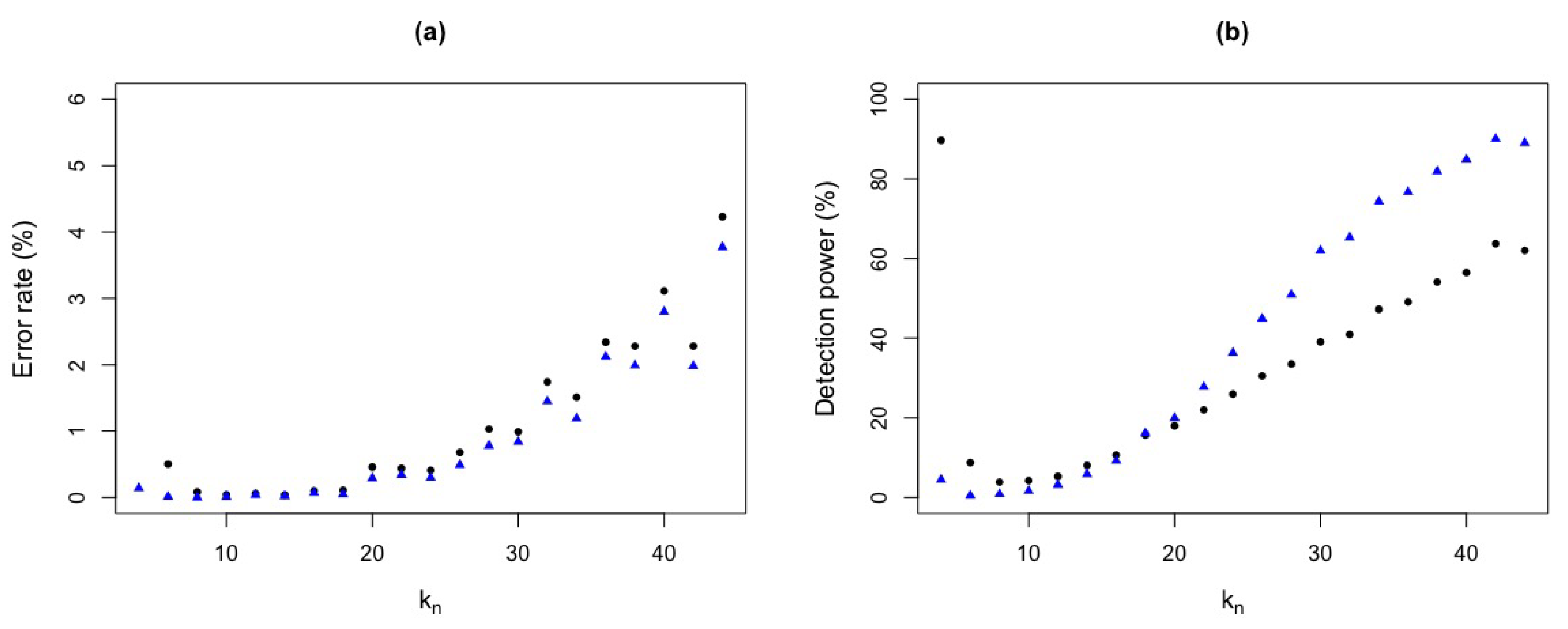
Figure 9.
Error rate and detection power with critical value and different values with . (a) Error rates for (black circle) and (blue triangle) test statistics. (b) Detection powers for (black circle) and (blue triangle) test statistics.
Figure 9.
Error rate and detection power with critical value and different values with . (a) Error rates for (black circle) and (blue triangle) test statistics. (b) Detection powers for (black circle) and (blue triangle) test statistics.
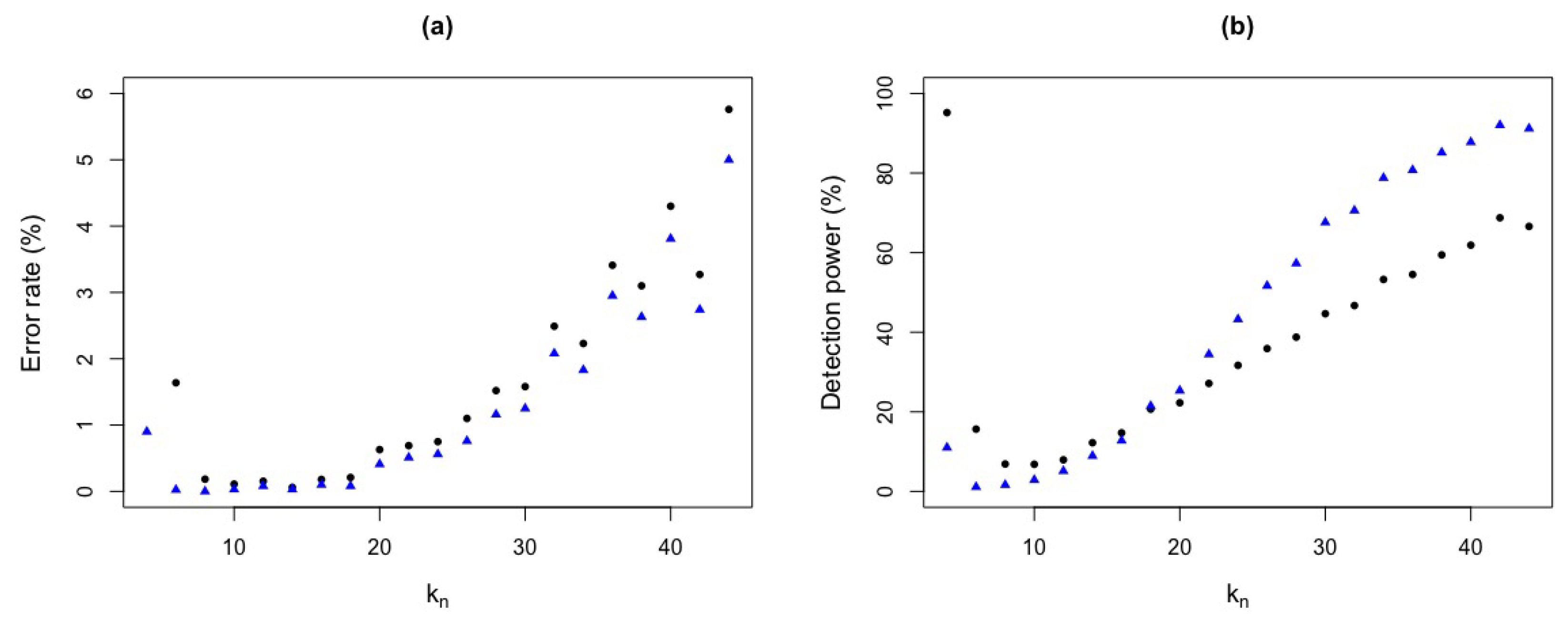
Figure 10.
ROC curve for and test statistics for Figure 9. (a) ROC curve . (b) ROC curve .
Figure 10.
ROC curve for and test statistics for Figure 9. (a) ROC curve . (b) ROC curve .
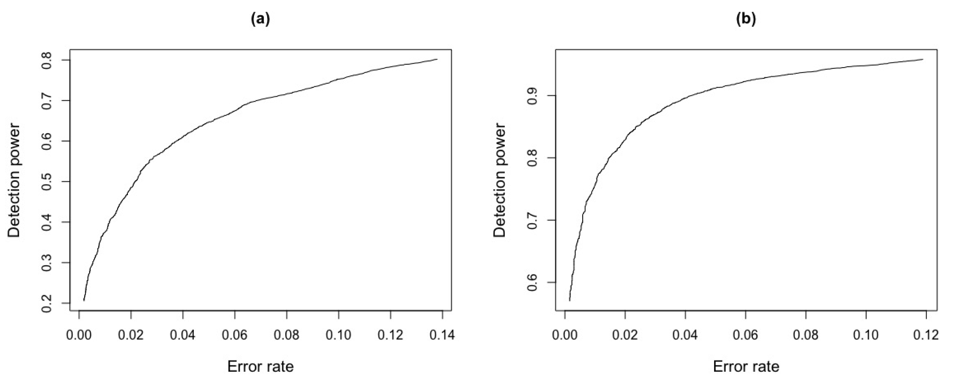
Figure 11.
MSD of test statistics for different values, in data generated from the jump-diffusion (blue triangle) and standard normal (black circle) models with .
Figure 11.
MSD of test statistics for different values, in data generated from the jump-diffusion (blue triangle) and standard normal (black circle) models with .
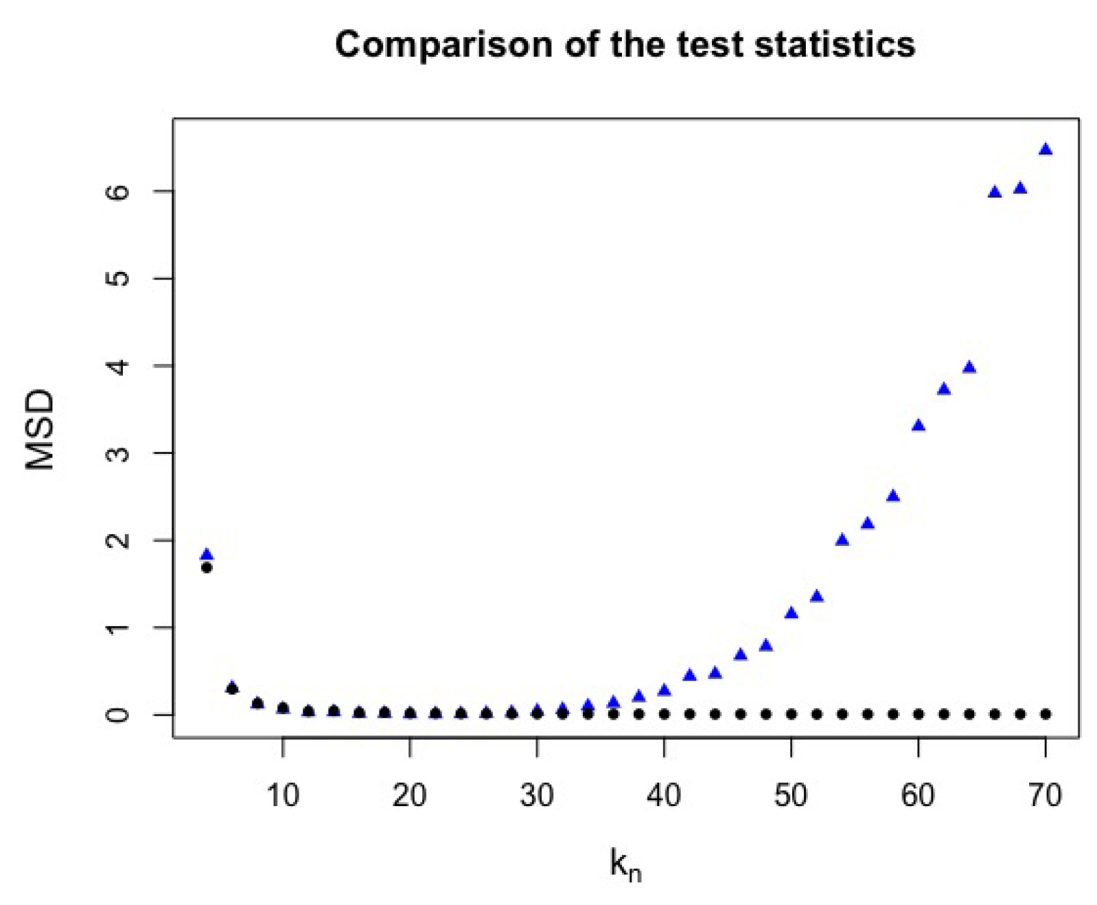
Figure 12.
Error rate and detection power with critical value and different values with . (a) Error rates for (black circle) and (blue triangle) test statistics. (b) Detection powers for (black circle) and (blue triangle) test statistics.
Figure 12.
Error rate and detection power with critical value and different values with . (a) Error rates for (black circle) and (blue triangle) test statistics. (b) Detection powers for (black circle) and (blue triangle) test statistics.
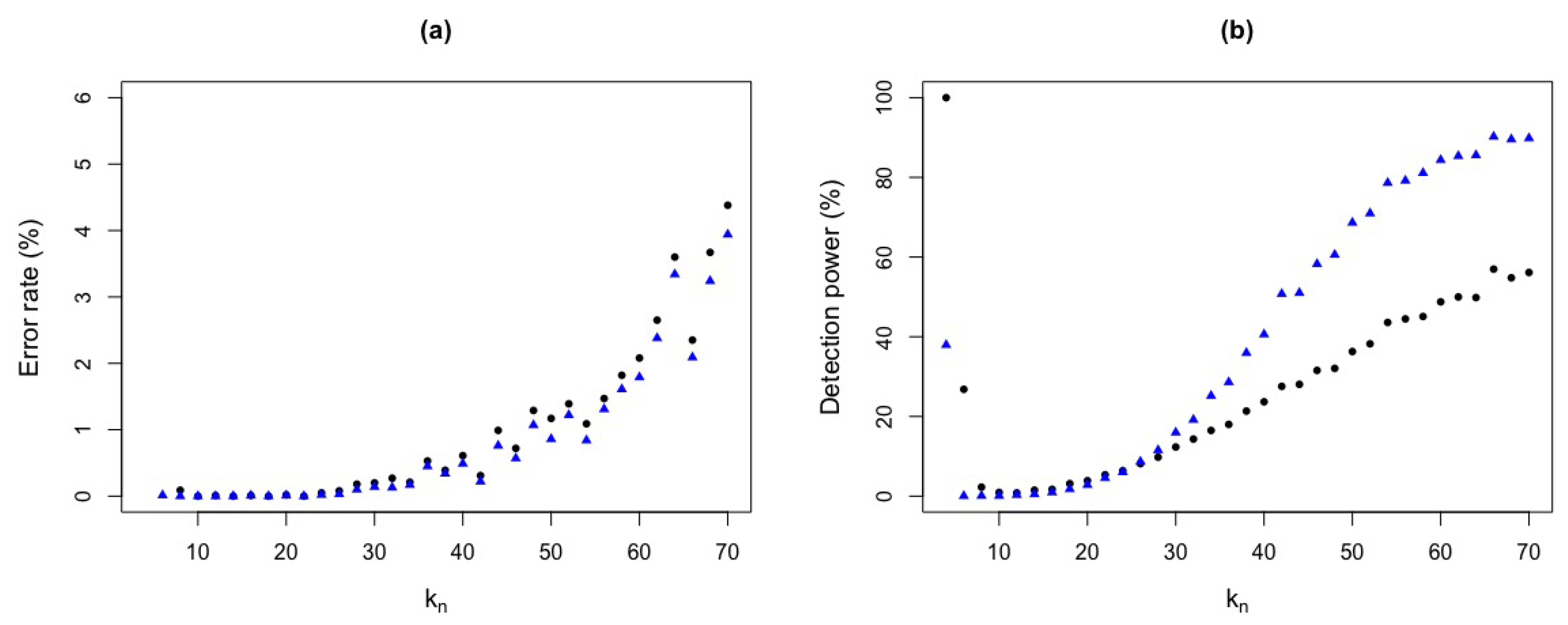
Figure 13.
Error rate and detection power with critical value and different values with . (a) Error rates for (black circle) and (blue triangle) test statistics. (b) Detection powers for (black circle) and (blue triangle) test statistics.
Figure 13.
Error rate and detection power with critical value and different values with . (a) Error rates for (black circle) and (blue triangle) test statistics. (b) Detection powers for (black circle) and (blue triangle) test statistics.
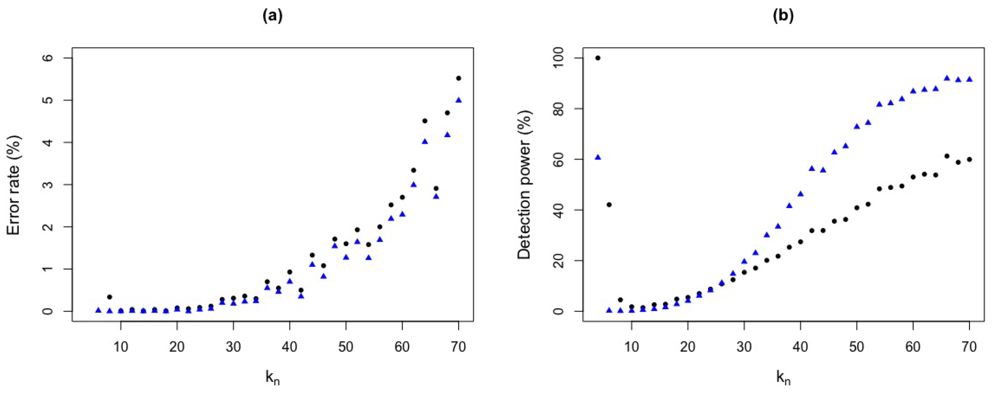
Figure 14.
ROC curve for and test statistics for Figure 13. (a) ROC curve . (b) ROC curve .
Figure 14.
ROC curve for and test statistics for Figure 13. (a) ROC curve . (b) ROC curve .
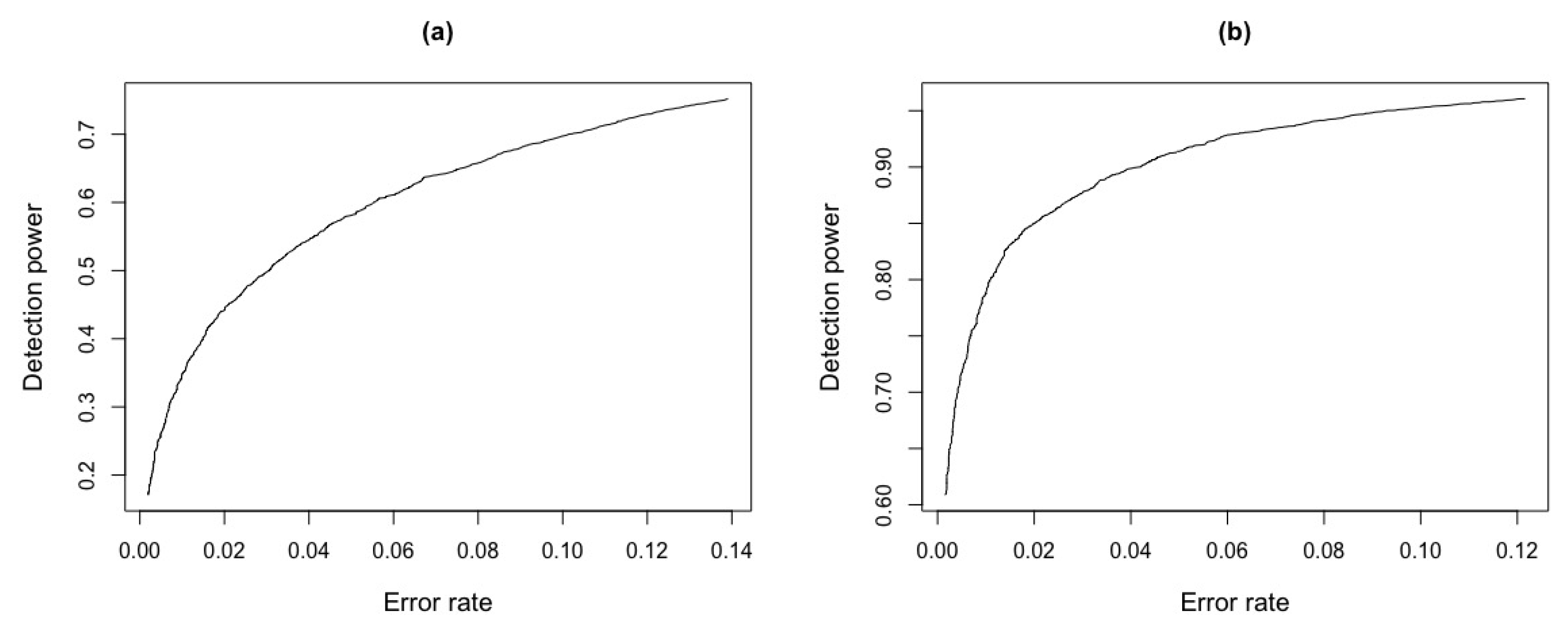
Figure 15.
Comparison between the edf of (black curve) and the gamma distribution function (red curve) for different and sample sizes n. (a) . (b) . (c) . (d) . (e) .
Figure 15.
Comparison between the edf of (black curve) and the gamma distribution function (red curve) for different and sample sizes n. (a) . (b) . (c) . (d) . (e) .
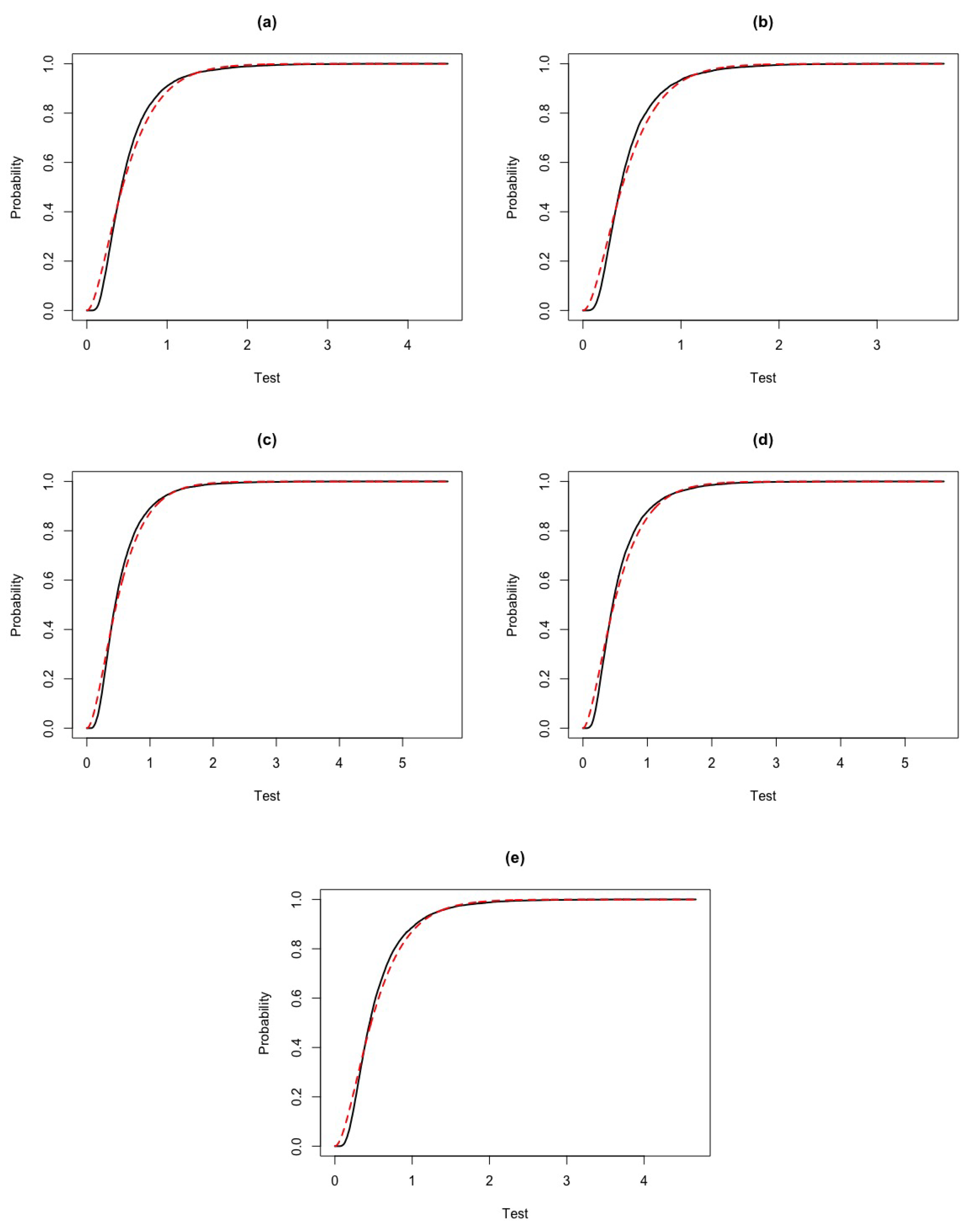
Figure 16.
Histograms of the edf of TA2 for different and sample sizes, n, compared with the gamma density (black curve). (a) . (b) . (c) . (d) . (e) . (f) . (g) . (h) . (i) .
Figure 16.
Histograms of the edf of TA2 for different and sample sizes, n, compared with the gamma density (black curve). (a) . (b) . (c) . (d) . (e) . (f) . (g) . (h) . (i) .
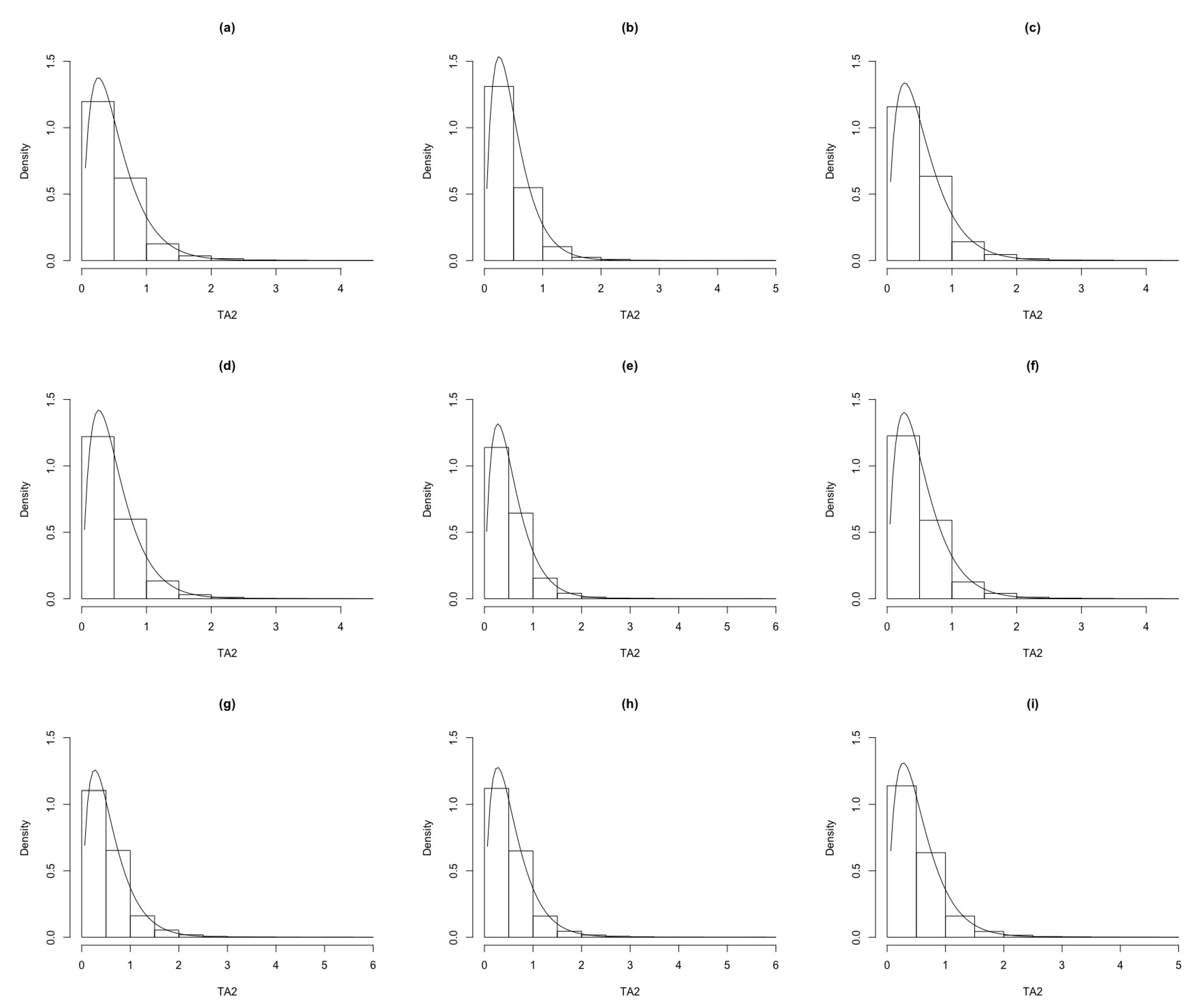
Figure 17.
Data generated from the jump-diffusion and standard normal models. (a) Jump-difussion model. (b) Standard normal model.
Figure 17.
Data generated from the jump-diffusion and standard normal models. (a) Jump-difussion model. (b) Standard normal model.
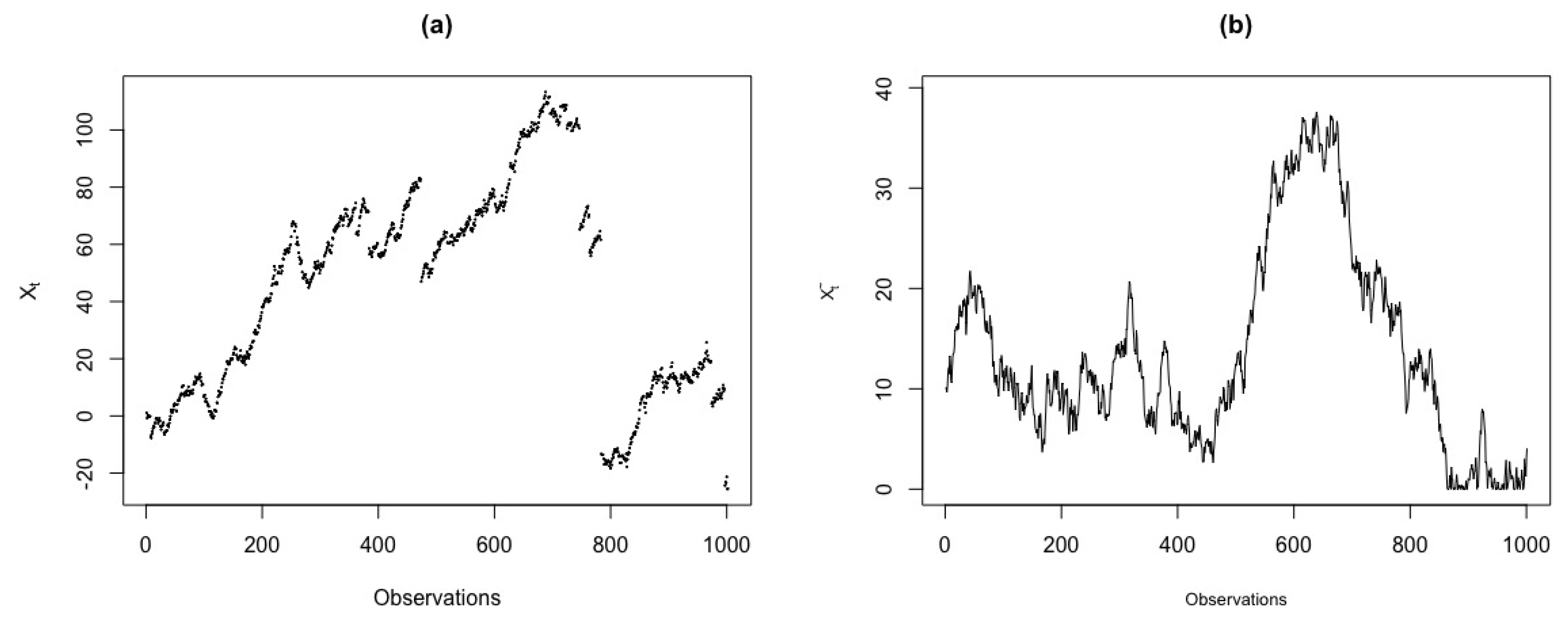
Figure 18.
Price series for market data of Apple, Google and GS stocks with transactions from 9:30 a.m to 4:00 p.m. (a) Apple. (b) Google. (c) GS.
Figure 18.
Price series for market data of Apple, Google and GS stocks with transactions from 9:30 a.m to 4:00 p.m. (a) Apple. (b) Google. (c) GS.
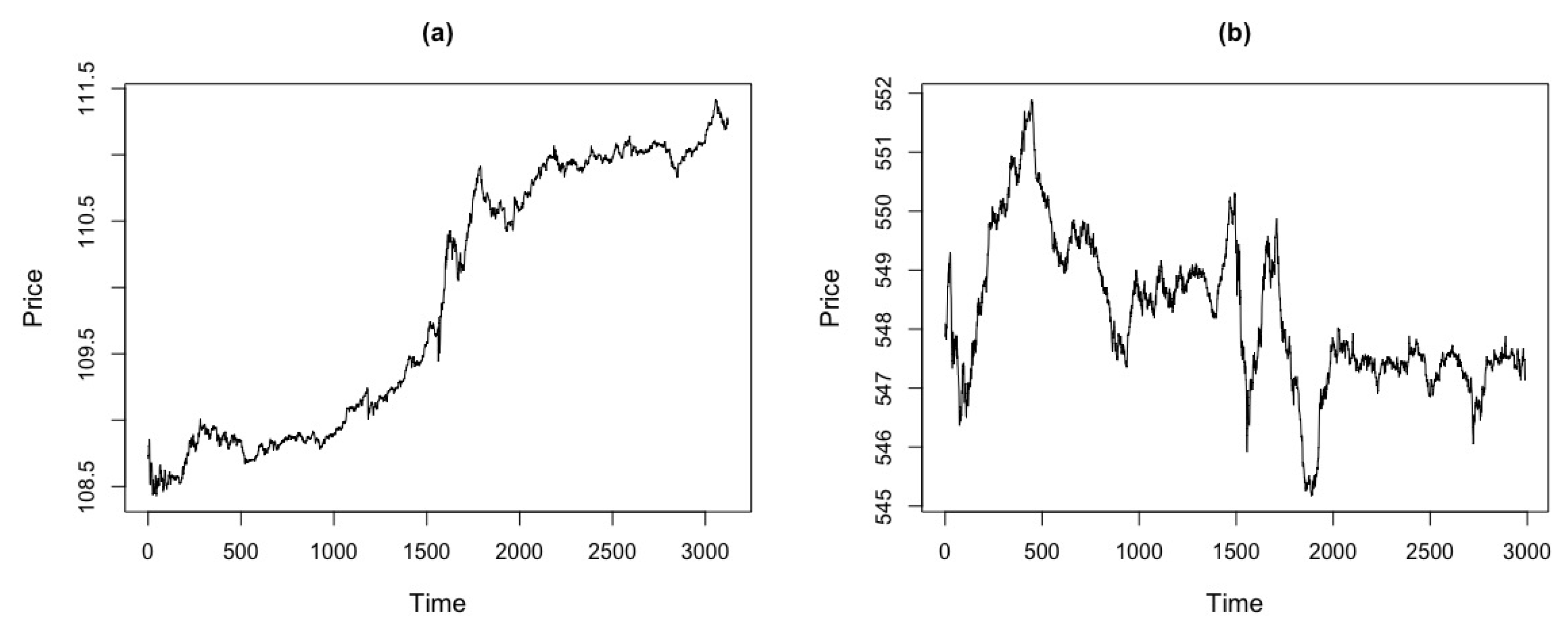
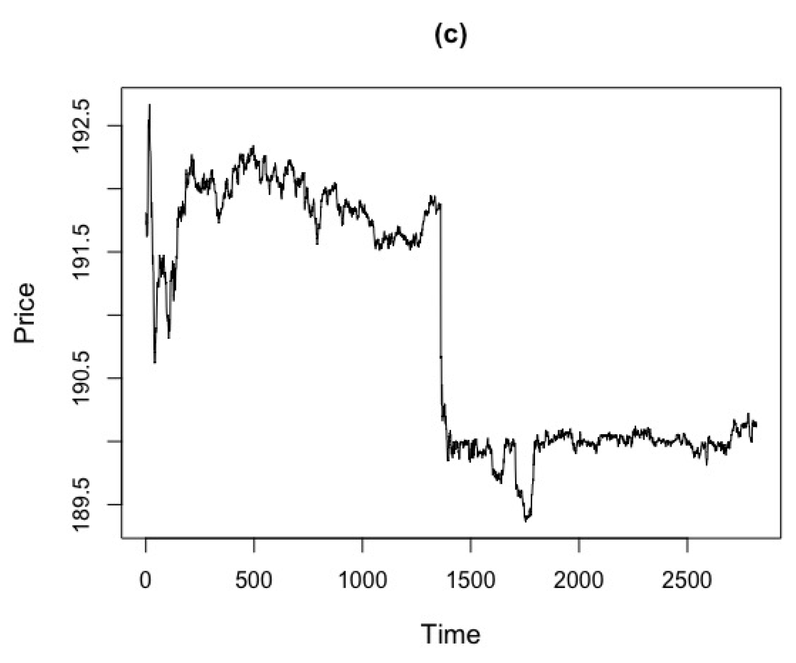
Figure 19.
test statistic, compared to different values for Apple, Google and GS stocks. (a) Apple, . (b) Apple, . (c) Google, . (d) Google, . (e) GS, . (f) GS, .
Figure 19.
test statistic, compared to different values for Apple, Google and GS stocks. (a) Apple, . (b) Apple, . (c) Google, . (d) Google, . (e) GS, . (f) GS, .
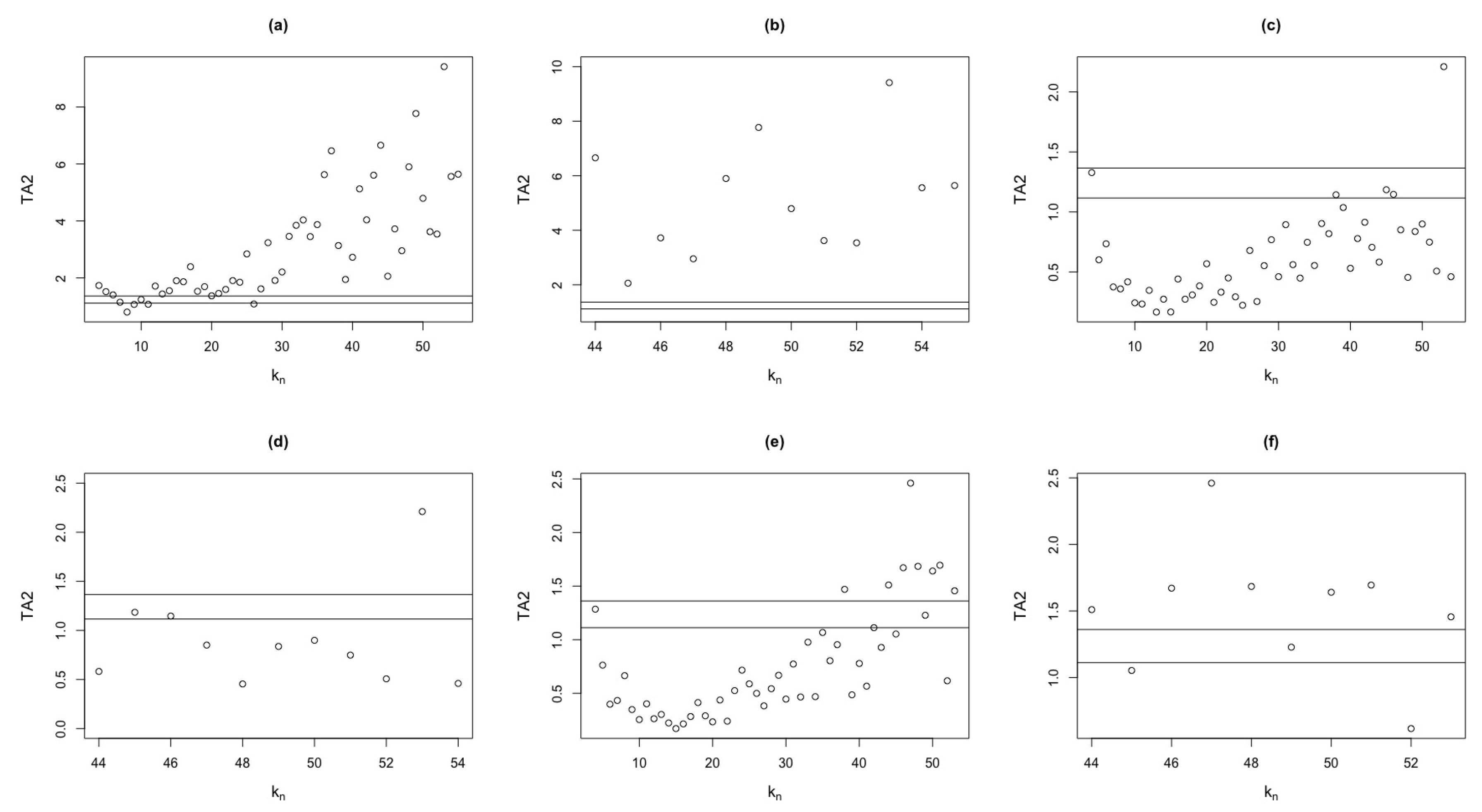

Table 1.
Error rates and detection powers for values between 4 and 30, a fixed critical value and the simulated critical value , in replicas of data generated with .
Table 1.
Error rates and detection powers for values between 4 and 30, a fixed critical value and the simulated critical value , in replicas of data generated with .
| Error rate | Detection power | Error rate | Detection power | ||||||
| 4 | 2 | 0.2728 | 0.0002 | 0.6026 | 0.0376 | 0.5286 | 0.0052 | 0.8217 | 0.1453 |
| 6 | 3 | 0.0029 | 0.0001 | 0.0952 | 0.0193 | 0.0204 | 0.0004 | 0.2378 | 0.0604 |
| 8 | 4 | 0.0015 | 0.0004 | 0.0805 | 0.0330 | 0.0056 | 0.0010 | 0.1793 | 0.0863 |
| 10 | 5 | 0.0011 | 0.0003 | 0.1061 | 0.0643 | 0.0057 | 0.0008 | 0.2074 | 0.1402 |
| 12 | 5 | 0.0042 | 0.0020 | 0.1372 | 0.1088 | 0.0100 | 0.0052 | 0.2324 | 0.1993 |
| 14 | 8 | 0.0014 | 0.0006 | 0.2071 | 0.1982 | 0.0054 | 0.0028 | 0.3248 | 0.3242 |
| 16 | 7 | 0.0060 | 0.0040 | 0.2323 | 0.2551 | 0.0164 | 0.0113 | 0.3490 | 0.3833 |
| 18 | 11 | 0.0039 | 0.0030 | 0.3204 | 0.4066 | 0.0110 | 0.0082 | 0.4578 | 0.5502 |
| 20 | 9 | 0.0140 | 0.0101 | 0.3381 | 0.4465 | 0.0287 | 0.0213 | 0.4616 | 0.5796 |
| 22 | 11 | 0.0149 | 0.0113 | 0.3984 | 0.5568 | 0.0306 | 0.0247 | 0.5208 | 0.6814 |
| 24 | 12 | 0.0164 | 0.0125 | 0.4569 | 0.6501 | 0.0354 | 0.0258 | 0.5795 | 0.7586 |
| 26 | 13 | 0.0231 | 0.0198 | 0.5094 | 0.7286 | 0.0451 | 0.0378 | 0.6255 | 0.8170 |
| 28 | 13 | 0.0309 | 0.0258 | 0.5378 | 0.7675 | 0.0585 | 0.0482 | 0.6472 | 0.8477 |
| 30 | 16 | 0.0305 | 0.0272 | 0.5989 | 0.8390 | 0.0599 | 0.0500 | 0.7057 | 0.8937 |
Table 2.
Error rates and detection powers for values between 4 and 44, a fixed critical value and, the simulated critical value , in replicas of data generated with .
Table 2.
Error rates and detection powers for values between 4 and 44, a fixed critical value and, the simulated critical value , in replicas of data generated with .
| Error rate | Detection power | Error rate | Detection power | ||||||
| 4 | 2 | 0.7289 | 0.0014 | 0.8966 | 0.0449 | 0.8380 | 0.0090 | 0.9519 | 0.1101 |
| 6 | 3 | 0.0050 | 0.0001 | 0.0877 | 0.0049 | 0.0164 | 0.0002 | 0.1565 | 0.0110 |
| 8 | 4 | 0.0008 | 0.0000 | 0.0387 | 0.0090 | 0.0018 | 0.0000 | 0.0688 | 0.0162 |
| 10 | 5 | 0.0004 | 0.0001 | 0.0424 | 0.0168 | 0.0011 | 0.0003 | 0.0681 | 0.0288 |
| 12 | 5 | 0.0006 | 0.0004 | 0.0530 | 0.0316 | 0.0015 | 0.0008 | 0.0793 | 0.0512 |
| 14 | 8 | 0.0004 | 0.0002 | 0.0806 | 0.0587 | 0.0006 | 0.0003 | 0.1223 | 0.0892 |
| 16 | 7 | 0.0010 | 0.0007 | 0.1066 | 0.0926 | 0.0018 | 0.0010 | 0.1471 | 0.1277 |
| 18 | 11 | 0.0011 | 0.0005 | 0.1572 | 0.1615 | 0.0021 | 0.0008 | 0.2067 | 0.2145 |
| 20 | 9 | 0.0046 | 0.0029 | 0.1799 | 0.1992 | 0.0063 | 0.0041 | 0.2227 | 0.2533 |
| 22 | 11 | 0.0044 | 0.0034 | 0.2201 | 0.2779 | 0.0069 | 0.0051 | 0.2713 | 0.3444 |
| 24 | 12 | 0.0041 | 0.0030 | 0.2596 | 0.3635 | 0.0075 | 0.0056 | 0.3168 | 0.4325 |
| 26 | 13 | 0.0068 | 0.0049 | 0.3052 | 0.4489 | 0.0110 | 0.0076 | 0.3589 | 0.5166 |
| 28 | 13 | 0.0103 | 0.0078 | 0.3350 | 0.5095 | 0.0152 | 0.0116 | 0.3876 | 0.5730 |
| 30 | 16 | 0.0099 | 0.0084 | 0.3908 | 0.6201 | 0.0158 | 0.0125 | 0.4465 | 0.6761 |
| 32 | 15 | 0.0174 | 0.0145 | 0.4094 | 0.6527 | 0.0249 | 0.0208 | 0.4670 | 0.7058 |
| 34 | 18 | 0.0151 | 0.0119 | 0.4726 | 0.7428 | 0.0223 | 0.0183 | 0.5326 | 0.7878 |
| 36 | 17 | 0.0234 | 0.0212 | 0.4911 | 0.7673 | 0.0341 | 0.0295 | 0.5451 | 0.8075 |
| 38 | 20 | 0.0228 | 0.0199 | 0.5409 | 0.8189 | 0.0310 | 0.0263 | 0.5943 | 0.8515 |
| 40 | 20 | 0.0311 | 0.0280 | 0.5648 | 0.8483 | 0.0430 | 0.0381 | 0.6188 | 0.8776 |
| 42 | 26 | 0.0228 | 0.0198 | 0.6370 | 0.9004 | 0.0327 | 0.0274 | 0.6876 | 0.9205 |
| 44 | 21 | 0.0423 | 0.0377 | 0.6201 | 0.8905 | 0.0576 | 0.0500 | 0.6659 | 0.9118 |
Table 3.
Error rates and detection powers for values between 4 and 70, a fixed critical value and the simulated critical value , in replicas of data generated with .
Table 3.
Error rates and detection powers for values between 4 and 70, a fixed critical value and the simulated critical value , in replicas of data generated with .
| Error rate | Detection power | Error rate | Detection power | ||||||
| 4 | 2 | 1.0000 | 0.1851 | 1.0000 | 0.3794 | 1.0000 | 0.4053 | 1.0000 | 0.6061 |
| 6 | 3 | 0.1101 | 0.0001 | 0.2681 | 0.0005 | 0.2176 | 0.0001 | 0.4208 | 0.0022 |
| 8 | 4 | 0.0009 | 0.0000 | 0.0226 | 0.0010 | 0.0034 | 0.0000 | 0.0452 | 0.0013 |
| 10 | 5 | 0.0000 | 0.0000 | 0.0094 | 0.0009 | 0.0001 | 0.0000 | 0.0179 | 0.0019 |
| 12 | 5 | 0.0001 | 0.0000 | 0.0082 | 0.0031 | 0.0004 | 0.0001 | 0.0145 | 0.0052 |
| 14 | 8 | 0.0000 | 0.0000 | 0.0150 | 0.0048 | 0.0001 | 0.0000 | 0.0261 | 0.0087 |
| 16 | 7 | 0.0001 | 0.0001 | 0.0171 | 0.0096 | 0.0004 | 0.0001 | 0.0279 | 0.0159 |
| 18 | 11 | 0.0000 | 0.0000 | 0.0314 | 0.0177 | 0.0001 | 0.0000 | 0.0481 | 0.0281 |
| 20 | 9 | 0.0002 | 0.0001 | 0.0387 | 0.0282 | 0.0008 | 0.0004 | 0.0548 | 0.0413 |
| 22 | 11 | 0.0000 | 0.0000 | 0.0536 | 0.0455 | 0.0006 | 0.0000 | 0.0699 | 0.0613 |
| 24 | 12 | 0.0005 | 0.0002 | 0.0638 | 0.0602 | 0.0009 | 0.0004 | 0.0875 | 0.0826 |
| 26 | 13 | 0.0008 | 0.0003 | 0.0815 | 0.0864 | 0.0012 | 0.0006 | 0.1080 | 0.1115 |
| 28 | 13 | 0.0018 | 0.0010 | 0.0978 | 0.1153 | 0.0028 | 0.0020 | 0.1246 | 0.1479 |
| 30 | 16 | 0.0020 | 0.0014 | 0.1233 | 0.1597 | 0.0031 | 0.0018 | 0.1538 | 0.1954 |
| 32 | 15 | 0.0027 | 0.0013 | 0.1432 | 0.1917 | 0.0036 | 0.0023 | 0.1705 | 0.2296 |
| 34 | 18 | 0.0021 | 0.0017 | 0.1649 | 0.2518 | 0.0030 | 0.0024 | 0.2011 | 0.2998 |
| 36 | 17 | 0.0053 | 0.0045 | 0.1800 | 0.2860 | 0.0070 | 0.0055 | 0.2174 | 0.3341 |
| 38 | 20 | 0.0039 | 0.0034 | 0.2135 | 0.3594 | 0.0055 | 0.0046 | 0.2530 | 0.4150 |
| 40 | 20 | 0.0061 | 0.0049 | 0.2368 | 0.4059 | 0.0093 | 0.0070 | 0.2742 | 0.4615 |
| 42 | 26 | 0.0031 | 0.0022 | 0.2755 | 0.5076 | 0.0050 | 0.0035 | 0.3185 | 0.5618 |
| 44 | 21 | 0.0099 | 0.0076 | 0.2806 | 0.5101 | 0.0133 | 0.0110 | 0.3189 | 0.5559 |
| 46 | 25 | 0.0072 | 0.0057 | 0.3156 | 0.5826 | 0.0108 | 0.0082 | 0.3556 | 0.6267 |
| 48 | 23 | 0.0129 | 0.0107 | 0.3206 | 0.6058 | 0.0171 | 0.0154 | 0.3626 | 0.6514 |
| 50 | 28 | 0.0117 | 0.0086 | 0.3629 | 0.6863 | 0.0160 | 0.0127 | 0.4086 | 0.7277 |
| 52 | 27 | 0.0139 | 0.0122 | 0.3823 | 0.7097 | 0.0193 | 0.0164 | 0.4226 | 0.7437 |
| 54 | 34 | 0.0109 | 0.0084 | 0.4359 | 0.7863 | 0.0158 | 0.0126 | 0.4834 | 0.8156 |
| 56 | 31 | 0.0147 | 0.0131 | 0.4448 | 0.7919 | 0.0200 | 0.0169 | 0.4888 | 0.8212 |
| 58 | 30 | 0.0182 | 0.0161 | 0.4508 | 0.8111 | 0.0252 | 0.0219 | 0.4944 | 0.8371 |
| 60 | 34 | 0.0208 | 0.0179 | 0.4876 | 0.8437 | 0.0270 | 0.0229 | 0.5301 | 0.8677 |
| 62 | 33 | 0.0265 | 0.0238 | 0.4999 | 0.8536 | 0.0334 | 0.0299 | 0.5411 | 0.8743 |
| 64 | 30 | 0.0360 | 0.0334 | 0.4983 | 0.8557 | 0.0451 | 0.0401 | 0.5380 | 0.8770 |
| 66 | 40 | 0.0235 | 0.0209 | 0.5697 | 0.9022 | 0.0291 | 0.0271 | 0.6127 | 0.9186 |
| 68 | 35 | 0.0367 | 0.0324 | 0.5480 | 0.8955 | 0.0470 | 0.0417 | 0.5882 | 0.9123 |
| 70 | 33 | 0.0438 | 0.0394 | 0.5613 | 0.8982 | 0.0552 | 0.0499 | 0.5994 | 0.9140 |
Table 4.
Error rates and detection powers of test statistic, for a fixed critical value and optimal critical values, in some scenarios for n.
Table 4.
Error rates and detection powers of test statistic, for a fixed critical value and optimal critical values, in some scenarios for n.
| Optimal q | ||||||
|---|---|---|---|---|---|---|
| n | Error rate | Detection power | Error rate | Detection power | ||
| 1,000 | 30 | 16 | 0.0272 | 0.8390 | 0.05 | 0.8937 |
| 2,000 | 44 | 21 | 0.0377 | 0.8905 | 0.05 | 0.9118 |
| 5,000 | 70 | 33 | 0.0394 | 0.8982 | 0.049 | 0.9140 |
Table 5.
Comparison between empirical and true gamma quantiles, for values between 18 and 100 and, between 11 and 54, with large values for n.
Table 5.
Comparison between empirical and true gamma quantiles, for values between 18 and 100 and, between 11 and 54, with large values for n.
| empirical | ||||||
|---|---|---|---|---|---|---|
| n | a | b | quantile | quantile | ||
| 500 | 18 | 11 | 2.254 | 0.190 | 0.982 | 0.970 |
| 20 | 11 | 2.109 | 0.238 | 1.174 | 1.165 | |
| 22 | 12 | 1.938 | 0.274 | 1.273 | 1.243 | |
| 1,000 | 26 | 13 | 2.083 | 0.231 | 1.128 | 1.116 |
| 28 | 13 | 1.993 | 0.267 | 1.266 | 1.270 | |
| 30 | 19 | 2.064 | 0.228 | 1.106 | 1.084 | |
| 2,000 | 40 | 18 | 1.922 | 0.283 | 1.308 | 1.296 |
| 42 | 22 | 1.972 | 0.267 | 1.259 | 1.246 | |
| 44 | 22 | 1.953 | 0.282 | 1.320 | 1.304 | |
| 5,000 | 66 | 36 | 1.993 | 0.261 | 1.239 | 1.251 |
| 68 | 38 | 1.974 | 0.264 | 1.241 | 1.247 | |
| 70 | 34 | 1.885 | 0.308 | 1.403 | 1.380 | |
| 10,000 | 96 | 62 | 1.947 | 0.253 | 1.181 | 1.179 |
| 98 | 48 | 1.894 | 0.301 | 1.379 | 1.357 | |
| 100 | 54 | 1.972 | 0.284 | 1.334 | 1.322 |
Table 6.
Percentage points for . Entries in the table are x such that . The upper number in a double entry is the critical value calculated by using the gamma distribution; the lower is that bases on the sample distribution.
Table 6.
Percentage points for . Entries in the table are x such that . The upper number in a double entry is the critical value calculated by using the gamma distribution; the lower is that bases on the sample distribution.
| n | Percentage points for the following values of p: | n | |||||||||||||||
| 500 | 0.037 | 0.061 | 0.090 | 0.137 | 0.177 | 0.215 | 0.251 | 0.443 | 0.717 | 0.798 | 0.901 | 1.041 | 1.273 | 1.498 | 1.788 | 2.495 | 500 |
| 0.121 | 0.145 | 0.167 | 0.201 | 0.231 | 0.259 | 0.285 | 0.430 | 0.650 | 0.722 | 0.825 | 0.964 | 1.243 | 1.589 | 2.054 | 3.194 | ||
| 1,000 | 0.037 | 0.059 | 0.087 | 0.129 | 0.164 | 0.198 | 0.230 | 0.397 | 0.633 | 0.702 | 0.790 | 0.909 | 1.106 | 1.297 | 1.542 | 2.138 | 1,000 |
| 0.107 | 0.129 | 0.152 | 0.186 | 0.212 | 0.235 | 0.259 | 0.382 | 0.569 | 0.641 | 0.727 | 0.859 | 1.084 | 1.361 | 1.754 | 2.700 | ||
| 2,000 | 0.040 | 0.064 | 0.095 | 0.143 | 0.185 | 0.224 | 0.262 | 0.461 | 0.745 | 0.829 | 0.935 | 1.080 | 1.320 | 1.553 | 1.853 | 2.583 | 2,000 |
| 0.117 | 0.142 | 0.169 | 0.206 | 0.238 | 0.267 | 0.296 | 0.443 | 0.679 | 0.759 | 0.863 | 1.023 | 1.304 | 1.625 | 2.072 | 3.278 | ||
| 5,000 | 0.037 | 0.0624 | 0.096 | 0.145 | 0.189 | 0.230 | 0.270 | 0.482 | 0.785 | 0.875 | 0.989 | 1.145 | 1.403 | 1.654 | 1.978 | 2.769 | 5,000 |
| 0.119 | 0.148 | 0.176 | 0.217 | 0.250 | 0.279 | 0.306 | 0.463 | 0.712 | 0.794 | 0.907 | 1.090 | 1.380 | 1.693 | 2.235 | 3.403 | ||
| 10,000 | 0.040 | 0.066 | 0.097 | 0.147 | 0.189 | 0.228 | 0.267 | 0.468 | 0.754 | 0.840 | 0.947 | 1.093 | 1.334 | 1.569 | 1.871 | 2.606 | 10,000 |
| 0.118 | 0.141 | 0.169 | 0.209 | 0.242 | 0.270 | 0.298 | 0.449 | 0.692 | 0.770 | 0.880 | 1.045 | 1.322 | 1.610 | 2.048 | 3.252 | ||
Table 7.
Comparison of test power with gamma and empirical quantiles, with a significance level of .
Table 7.
Comparison of test power with gamma and empirical quantiles, with a significance level of .
| empirical | test | ||||||
|---|---|---|---|---|---|---|---|
| n | a | b | quantile | quantile | power | ||
| 500 | 4 | 2 | 6.323 | 0.087 | 0.962 | 0.905 | 0.564 |
| 6 | 3 | 2.302 | 0.165 | 0.865 | 0.689 | 0.615 | |
| 8 | 4 | 3.592 | 0.096 | 0.693 | 0.684 | 0.818 | |
| 18 | 11 | 2.254 | 0.190 | 0.982 | 0.968 | 0.956 | |
| 20 | 11 | 2.109 | 0.238 | 1.174 | 1.165 | 0.928 | |
| 22 | 12 | 1.938 | 0.274 | 1.273 | 1.243 | 0.930 | |
| 1,000 | 4 | 2 | 13.991 | 0.049 | 1.017 | 1.004 | 0.875 |
| 6 | 3 | 6.924 | 0.060 | 0.709 | 0.680 | 0.958 | |
| 8 | 4 | 5.350 | 0.064 | 0.623 | 0.621 | 0.981 | |
| 26 | 13 | 2.083 | 0.231 | 1.128 | 1.116 | 0.999 | |
| 28 | 13 | 1.993 | 0.267 | 1.266 | 1.270 | 0.997 | |
| 30 | 19 | 2.064 | 0.228 | 1.106 | 1.084 | 0.999 | |
| 2,000 | 4 | 2 | 27.702 | 0.032 | 1.202 | 1.196 | 0.990 |
| 6 | 3 | 14.850 | 0.033 | 0.736 | 0.731 | 0.999 | |
| 8 | 4 | 9.147 | 0.041 | 0.612 | 0.607 | 0.999 | |
| 40 | 18 | 1.922 | 0.283 | 1.308 | 1.296 | 1 | |
| 42 | 22 | 1.972 | 0.267 | 1.259 | 1.246 | 1 | |
| 44 | 22 | 1.953 | 0.282 | 1.320 | 1.304 | 1 | |
| 5,000 | 4 | 2 | 69.609 | 0.019 | 1.633 | 1.631 | 1 |
| 6 | 3 | 35.490 | 0.020 | 0.921 | 0.920 | 1 | |
| 8 | 4 | 21.383 | 0.023 | 0.694 | 0.694 | 1 | |
| 66 | 36 | 1.993 | 0.261 | 1.239 | 1.251 | 1 | |
| 68 | 38 | 1.974 | 0.264 | 1.241 | 1.247 | 1 | |
| 70 | 34 | 1.885 | 0.308 | 1.403 | 1.380 | 1 | |
| 10,000 | 4 | 2 | 132.233 | 0.014 | 2.155 | 2.154 | 1 |
| 6 | 3 | 70.155 | 0.013 | 1.171 | 1.170 | 1 | |
| 8 | 4 | 41.810 | 0.015 | 0.839 | 0.838 | 1 | |
| 96 | 62 | 1.947 | 0.253 | 1.181 | 1.179 | 1 | |
| 98 | 48 | 1.894 | 0.301 | 1.379 | 1.357 | 1 | |
| 100 | 54 | 1.972 | 0.284 | 1.334 | 1.322 | 1 |
Table 8.
Comparison between and KS test power, with a significance level of and large values for n.
| Gamma | sample | power | power | error | |||||
|---|---|---|---|---|---|---|---|---|---|
| n | a | b | quantile | KS | rate KS | ||||
| 500 | 4 | 2 | 6.323 | 0.087 | 0.962 | 0.905 | 0.564 | 0.958 | 0.763 |
| 6 | 3 | 2.302 | 0.165 | 0.865 | 0.689 | 0.615 | 0.958 | 0.963 | |
| 8 | 4 | 3.592 | 0.096 | 0.693 | 0.684 | 0.818 | 0.959 | 0.987 | |
| 18 | 11 | 2.254 | 0.190 | 0.982 | 0.968 | 0.956 | 0.960 | 0.999 | |
| 20 | 11 | 2.109 | 0.238 | 1.174 | 1.165 | 0.928 | 0.958 | 1 | |
| 22 | 12 | 1.938 | 0.274 | 1.273 | 1.243 | 0.930 | 0.960 | 1 | |
| 1,000 | 4 | 2 | 13.991 | 0.049 | 1.017 | 1.004 | 0.875 | 0.911 | 0.691 |
| 6 | 3 | 6.924 | 0.060 | 0.709 | 0.680 | 0.958 | 0.912 | 0.913 | |
| 8 | 4 | 5.350 | 0.064 | 0.623 | 0.621 | 0.981 | 0.911 | 0.974 | |
| 26 | 13 | 2.083 | 0.231 | 1.128 | 1.116 | 0.999 | 0.913 | 1 | |
| 28 | 13 | 1.993 | 0.267 | 1.266 | 1.270 | 0.997 | 0.914 | 1 | |
| 30 | 19 | 2.064 | 0.228 | 1.106 | 1.084 | 0.999 | 0.913 | 1 | |
| 2,000 | 4 | 2 | 27.702 | 0.032 | 1.202 | 1.196 | 0.990 | 0.836 | 0.528 |
| 6 | 3 | 14.850 | 0.033 | 0.736 | 0.731 | 0.999 | 0.836 | 0.897 | |
| 8 | 4 | 9.147 | 0.041 | 0.612 | 0.607 | 0.999 | 0.836 | 0.977 | |
| 40 | 18 | 1.922 | 0.283 | 1.308 | 1.296 | 1 | 0.836 | 1 | |
| 42 | 22 | 1.972 | 0.267 | 1.259 | 1.246 | 1 | 0.838 | 1 | |
| 44 | 22 | 1.953 | 0.282 | 1.320 | 1.304 | 1 | 0.837 | 1 | |
| 5,000 | 4 | 2 | 69.609 | 0.019 | 1.633 | 1.631 | 1 | 0.635 | 0.462 |
| 6 | 3 | 35.490 | 0.020 | 0.921 | 0.920 | 1 | 0.635 | 0.818 | |
| 8 | 4 | 21.383 | 0.023 | 0.694 | 0.694 | 1 | 0.635 | 0.959 | |
| 66 | 36 | 1.993 | 0.261 | 1.239 | 1.251 | 1 | 0.638 | 1 | |
| 68 | 38 | 1.974 | 0.264 | 1.241 | 1.247 | 1 | 0.637 | 1 | |
| 70 | 34 | 1.885 | 0.308 | 1.403 | 1.380 | 1 | 0.637 | 1 |
Table 9.
Rejection rates of test statistic, considering all possible values, with a significance level of and , for the three stock prices considered.
Table 9.
Rejection rates of test statistic, considering all possible values, with a significance level of and , for the three stock prices considered.
| Stock | n | ||||
|---|---|---|---|---|---|
| Apple | 3,122 | [4,55] | [2,27] | 88% | 92% |
| 2,989 | [4,54] | [2,27] | 2% | 10% | |
| GS | 2,819 | [4,53] | [2,26] | 16% | 20% |
Table 10.
Rejection rates of test statistic, considering values that are at least 44, with a significance level of and , for the three stock prices considered.
Table 10.
Rejection rates of test statistic, considering values that are at least 44, with a significance level of and , for the three stock prices considered.
| Stock | n | ||||
|---|---|---|---|---|---|
| Apple | 3,122 | [44,55] | [22,27] | 100% | 100% |
| 2,989 | [44,54] | [22,27] | 9% | 27% | |
| GS | 2,819 | [44,53] | [22,26] | 70% | 80% |
Disclaimer/Publisher’s Note: The statements, opinions and data contained in all publications are solely those of the individual author(s) and contributor(s) and not of MDPI and/or the editor(s). MDPI and/or the editor(s) disclaim responsibility for any injury to people or property resulting from any ideas, methods, instructions or products referred to in the content. |
© 2024 by the authors. Licensee MDPI, Basel, Switzerland. This article is an open access article distributed under the terms and conditions of the Creative Commons Attribution (CC BY) license (http://creativecommons.org/licenses/by/4.0/).
Copyright: This open access article is published under a Creative Commons CC BY 4.0 license, which permit the free download, distribution, and reuse, provided that the author and preprint are cited in any reuse.


