Submitted:
25 November 2024
Posted:
26 November 2024
You are already at the latest version
Abstract
This paper investigates multifractal cross-correlations and information flow among daily closing prices of stock-typical U.S. industry sectors, combining multifractal detrended cross-correlation analysis (MFDCCA), transfer entropy (TE), and complex network methods. Firstly, the ensemble empirical mode decomposition (EEMD) method estimates the dominant frequency. Then, the DCCA coefficient is computed, revealing that JPM exhibits nonlinear cross-correlations with all seven other stocks. Secondly, a more detailed examination using MFDCCA elucidates fractal characteristics. The experimental results reveal long-range and multiple fractal characteristics in the cross-correlations between JPM and the remaining seven stocks. Notably, the strongest multifractal cross-correlation is observed between JPM and XOM, while the weakest is between JPM and SPG. Thirdly, transfer entropy is calculated for each pair of the eight stocks to research the direction of information flow. The analysis reveals bidirectional information transfers, which are notable for the high information transfer from PG to XOM, as indicated by the transfer entropy matrix. Finally, utilizing a complex network approach to visualize the transfer entropy results, it is evident that AAPL possesses the most significant information outflow, while XOM exhibits the most substantial information inflow. These findings present critical insights beneficial for portfolio decision-making in the stock markets.
Keywords:
1. Introduction
2. Methodology
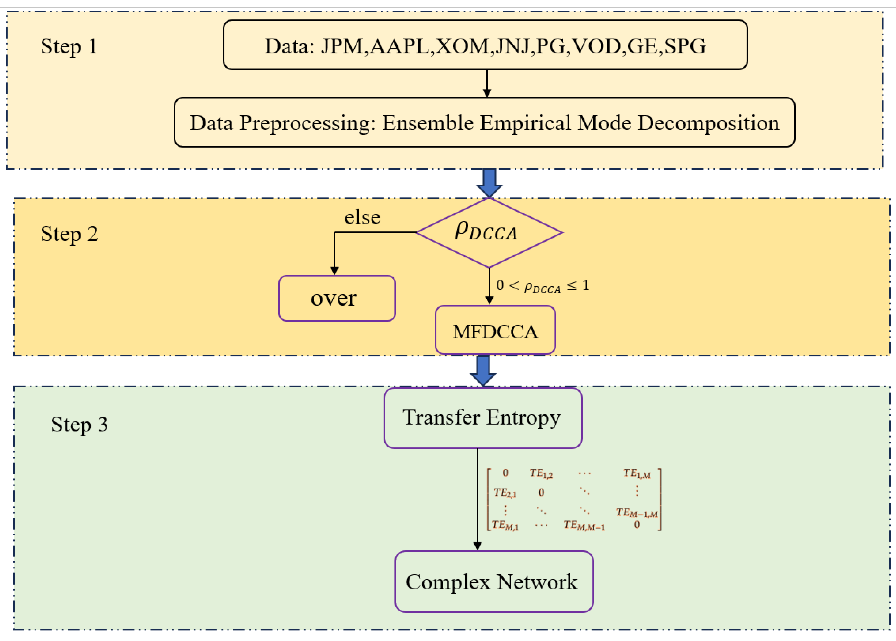
2.1. Multifractal Detrended Cross-Correlation Analysis–MFDCCA
| Algorithm 1: MFDCCA Method | |
| Step 1: | Consider two time series and , , and , where N is the length of the time series, , . |
| Step 2: | Partition the profiles and into non-overlapping segments of uniform length s. As the series length N is not required to be a multiple of the specified time scale s, a brief segment near the conclusion of the profiles may remain. The identical method is reiterated from the other end to incorporate this segment of the original series. Consequently, segments are acquired. |
| Step 3: | For each segment , where , the local trends and are determined by least-squares linear regression of the series. Consequently, for each segment , where , the covariance of the residuals is computed as follows: for each segment , . |
| Step 4: | Then, average over all segments to obtain the q-order fluctuation function. where the order q can take any real value. When , the algorithm becomes the standard detrended cross-correlation analysis (DCCA). |
| Step 5: | Ultimately, if two time series and exhibit long-range power-law cross-correlation, then , where is referred to as the generalized cross-correlation exponent. |
2.2. Transfer Entropy Based on KNN
2.3. Complex Networks
3. Data Description and Preprocessing
3.1. Data Description
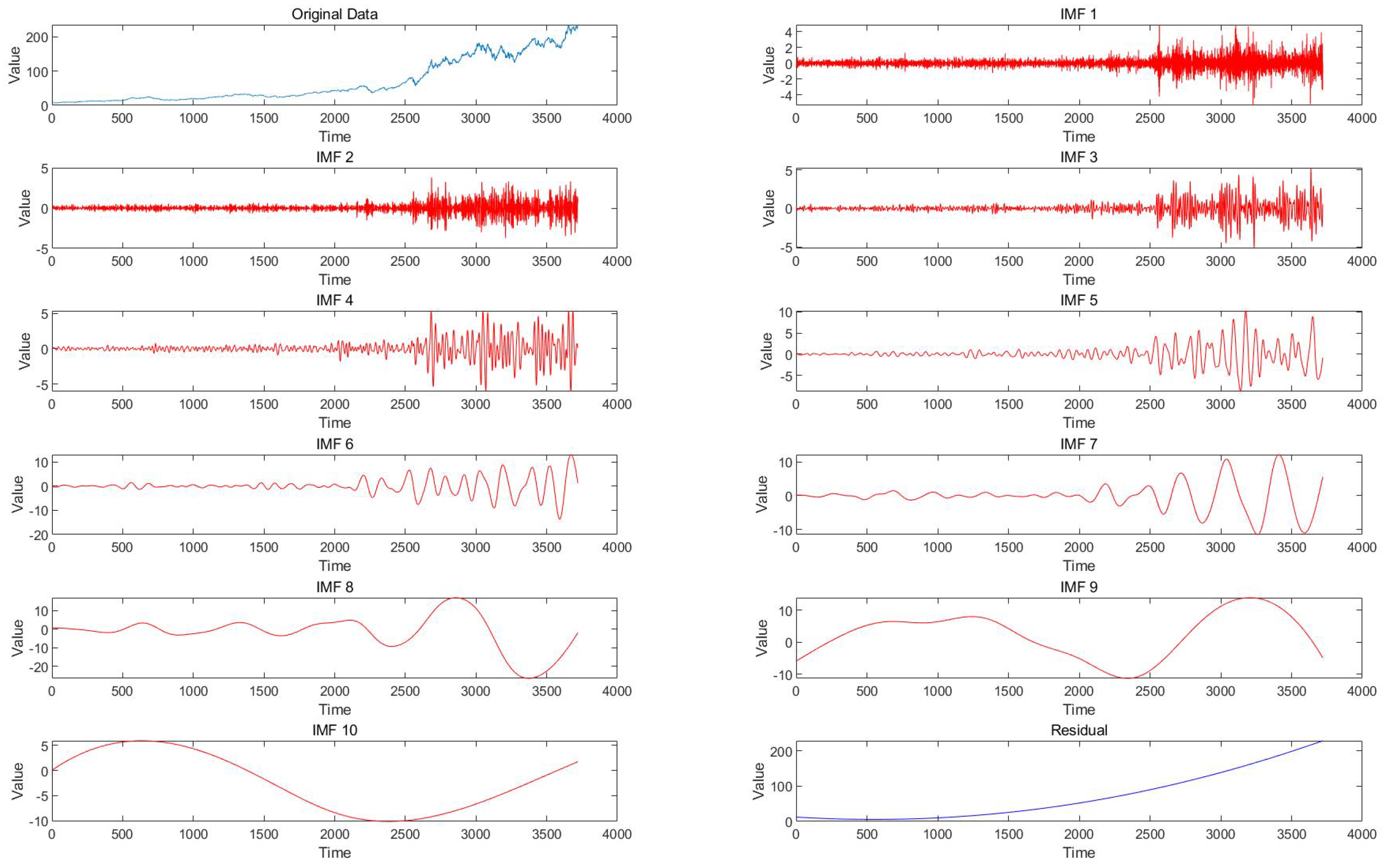
3.2. Data Preprocessing
| Algorithm 2: EEMD Method | |
| Step 1: | Add a group of white noise to form a new signal : |
| Step 2: | Perform EMD decomposition on to obtain n IMF components and a residual: |
| Step 3: | Add N groups of different white noises to the original time series signal and |
| repeat the previous steps: | |
| Step 4: | After EMD decomposition, the IMFs of each group can be expressed as follows: |
| Step 5: | The average value of the decomposed IMFs is obtained as the final result: |
| where is the jth IMF component obtained by EEMD decomposition of the | |
| original series. | |
4. Empirical Results
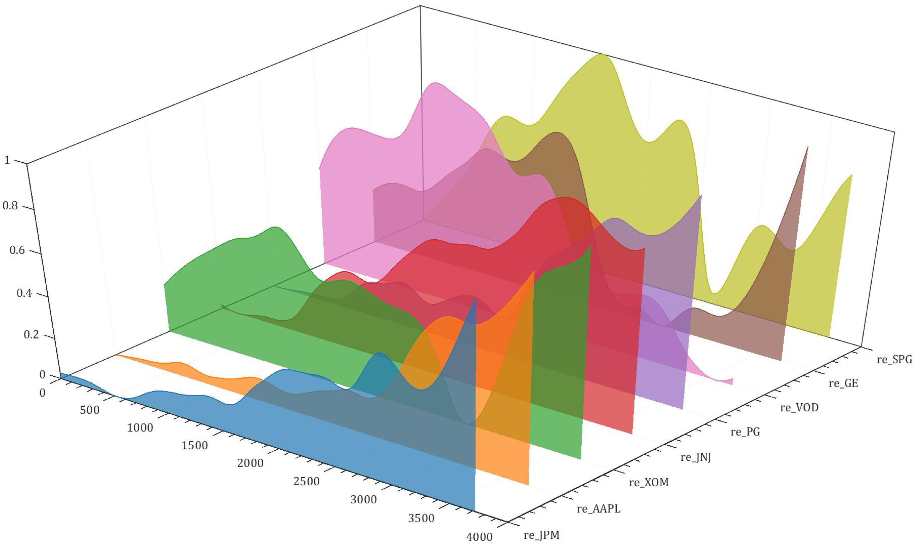
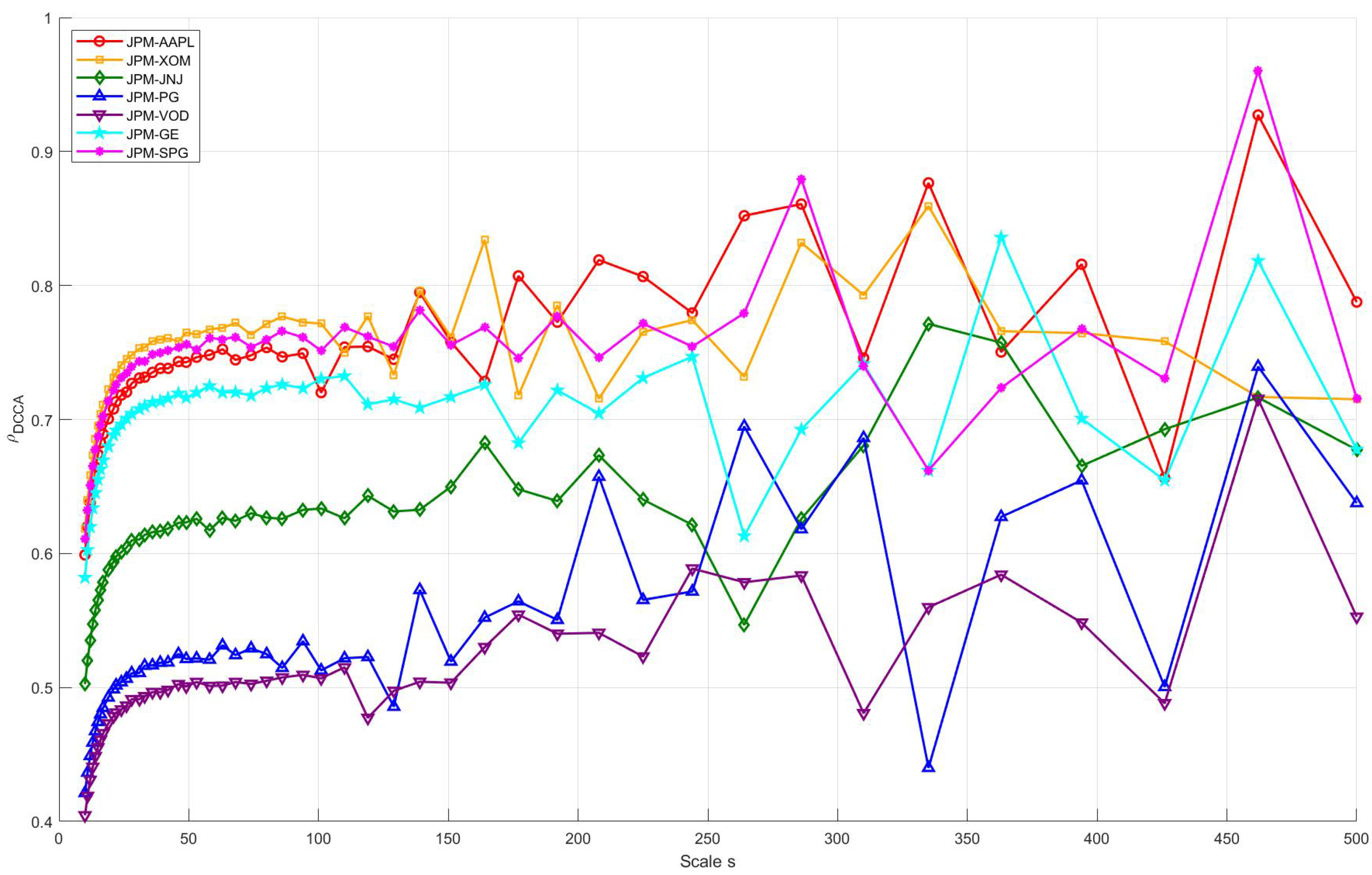
4.1. DCCA Coefficient
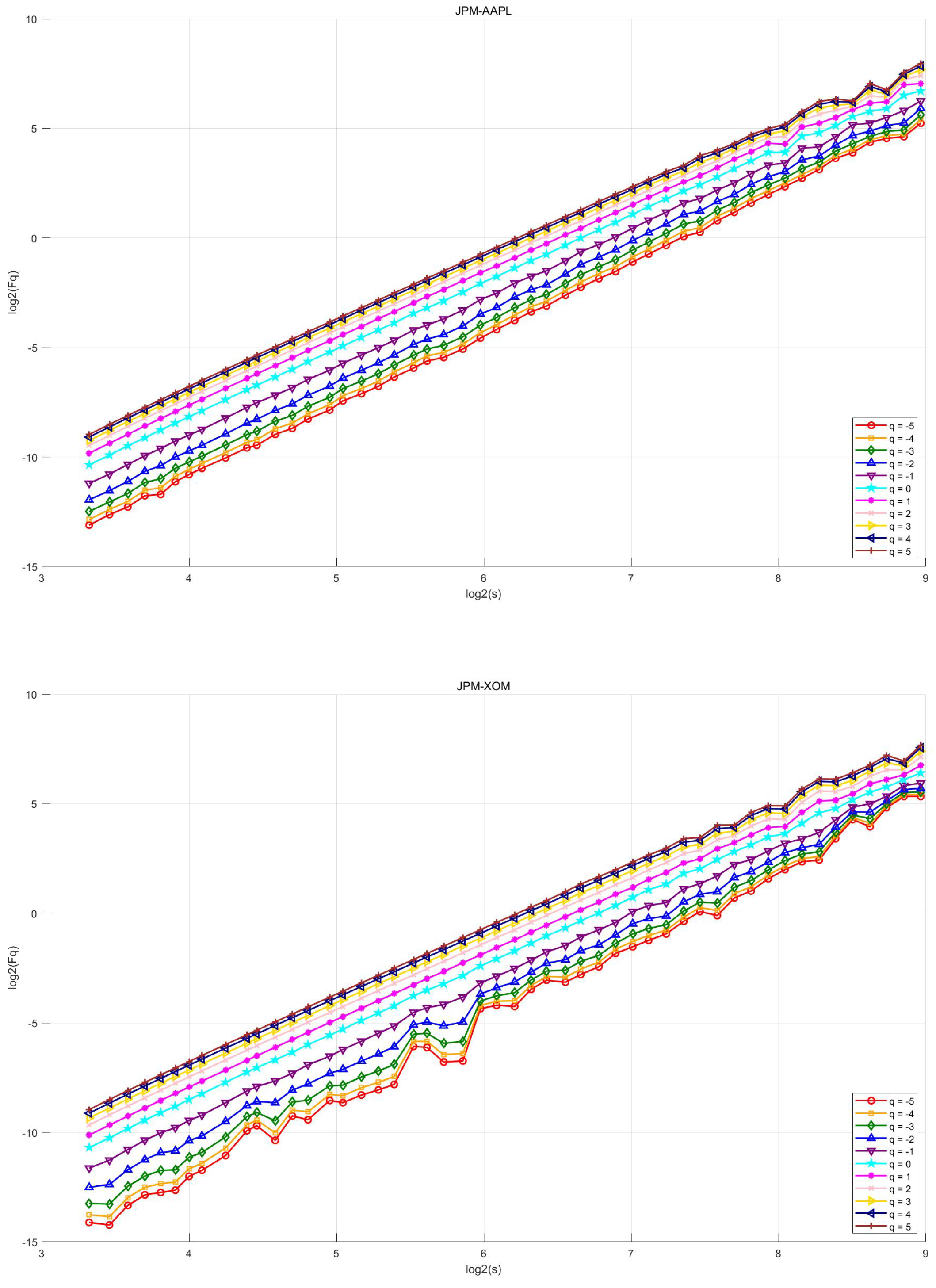
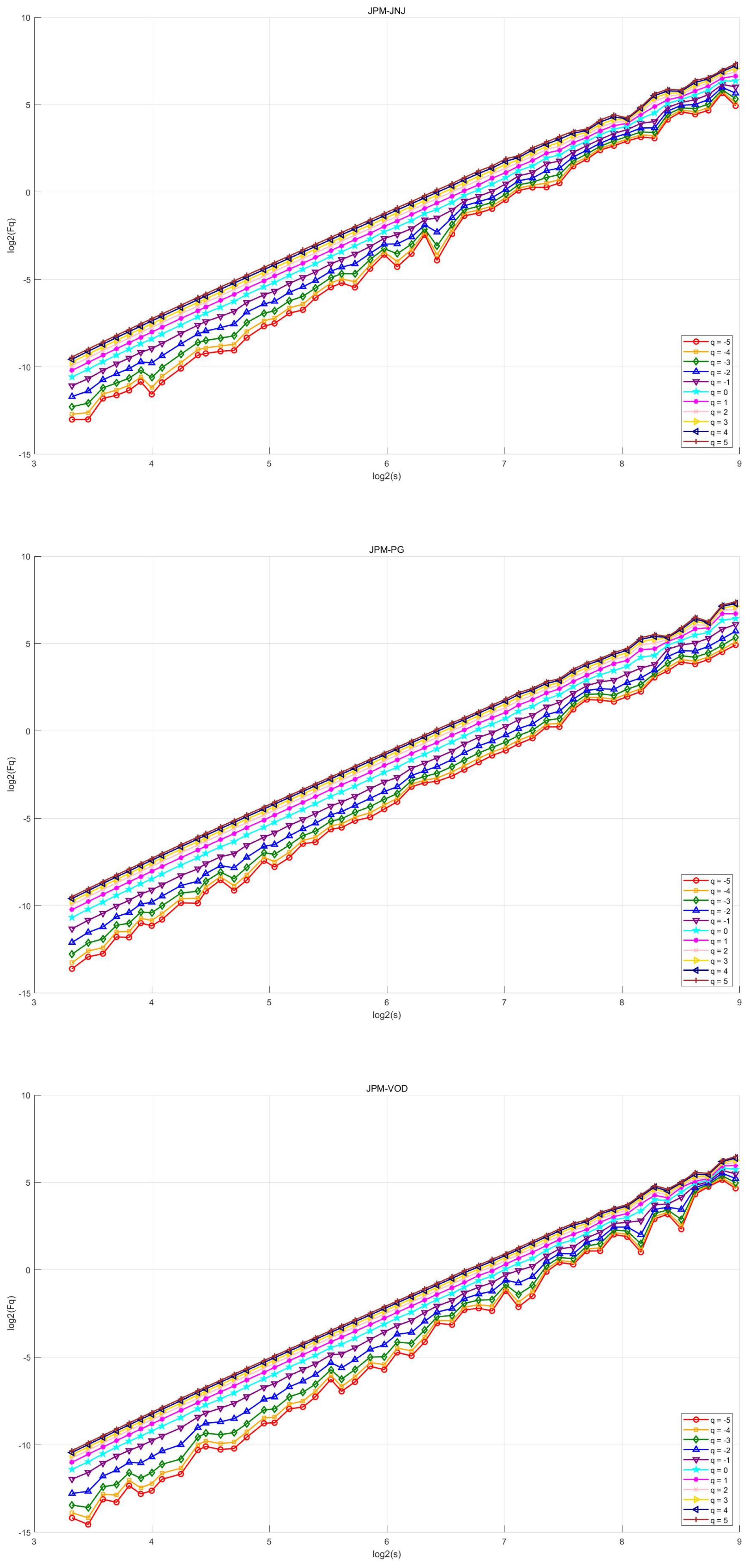
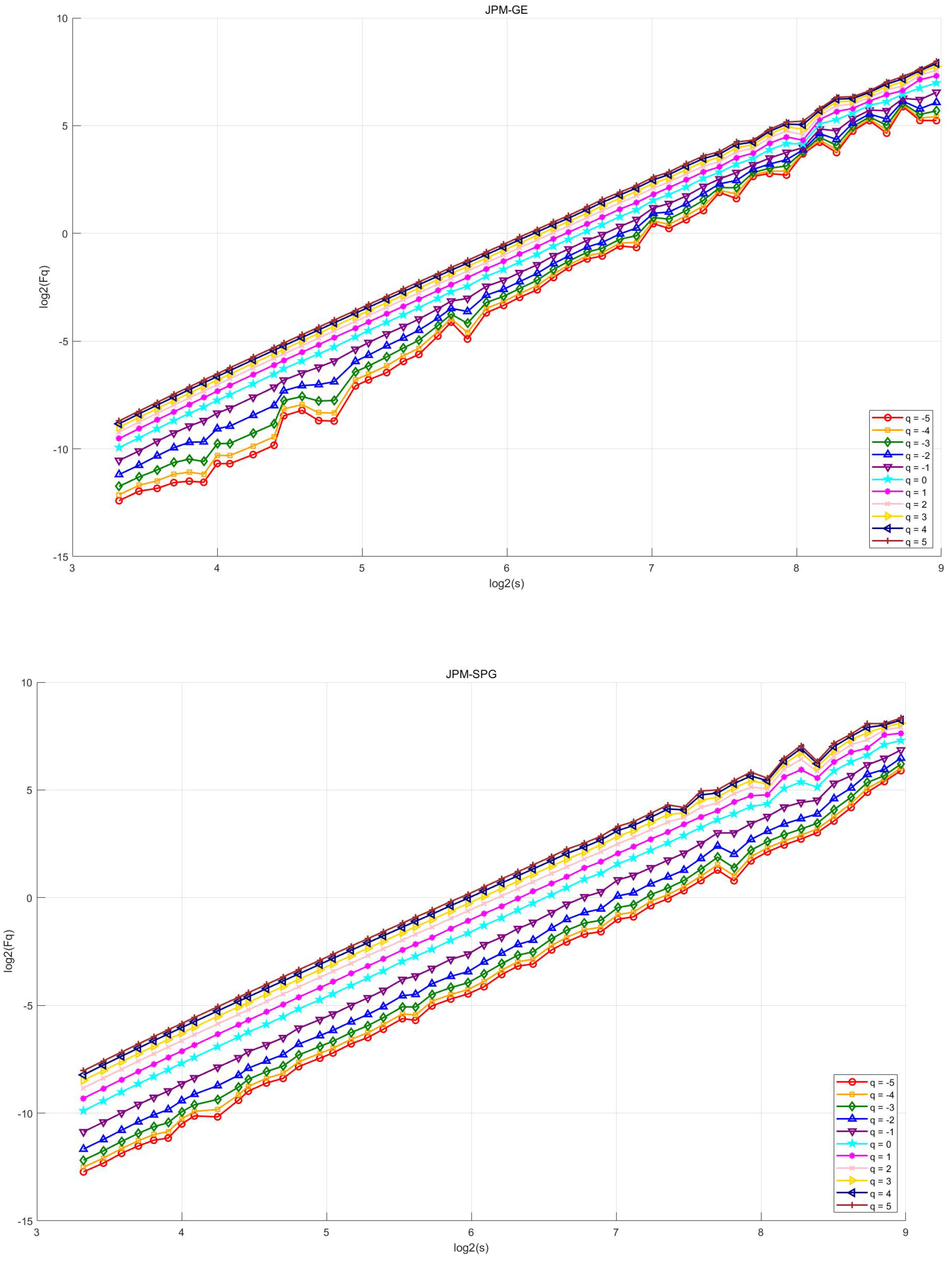
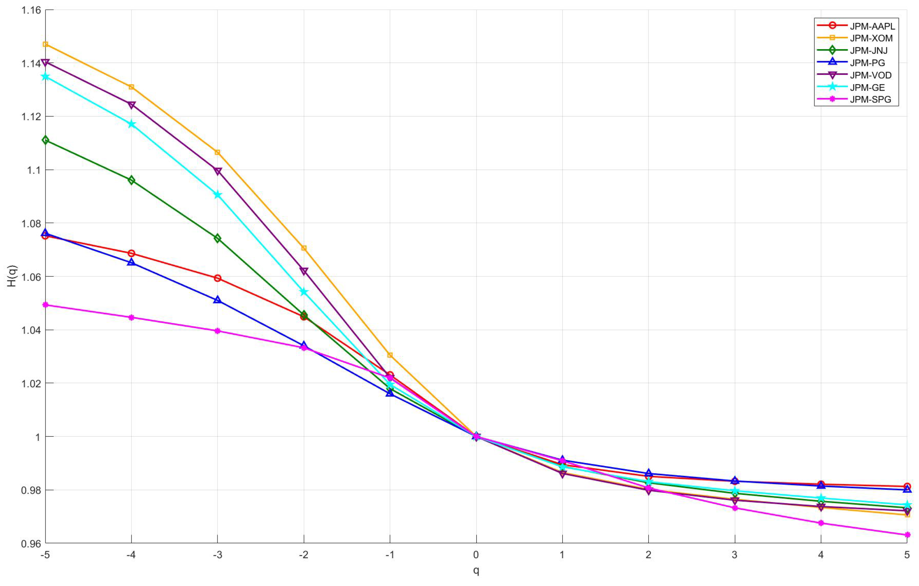
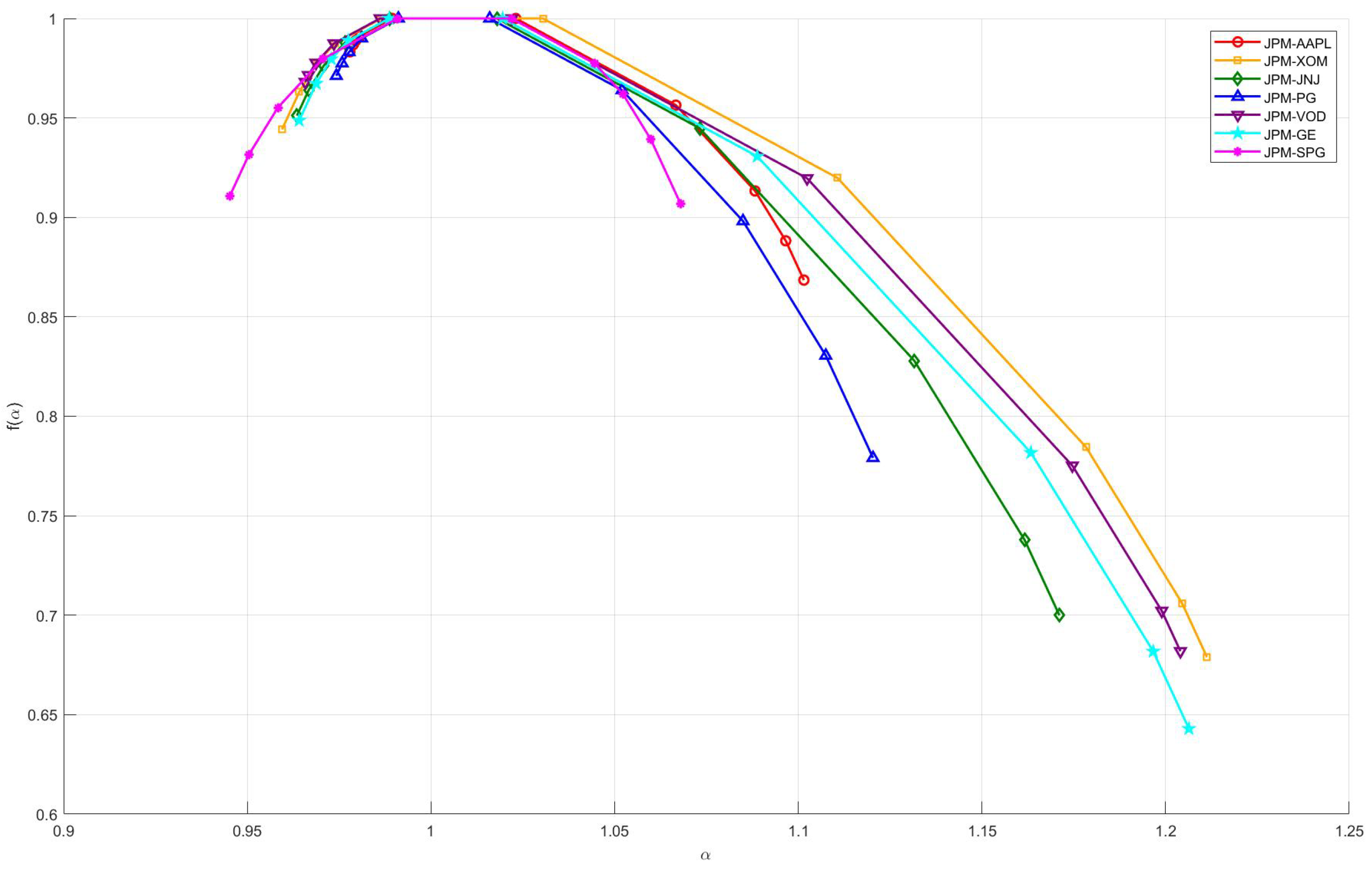
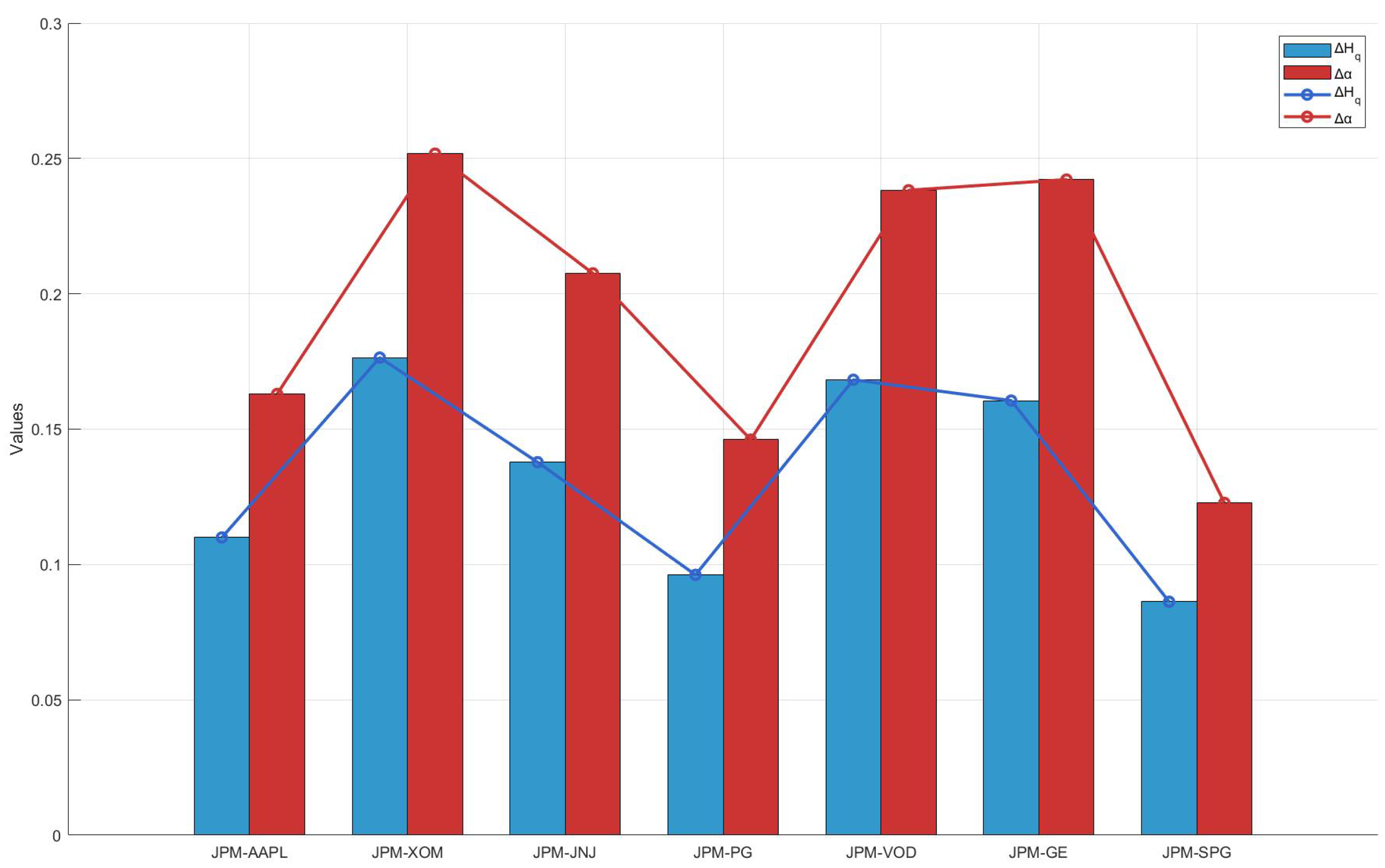
4.2. MFDCCA
4.3. TE Based on KNN
- JNJ→JPM, indicating that the healthcare industry sector has the most significant impact on the financial industry sector. This may reflect the healthcare sector’s stability and growth potential, attracting investment and attention from financial institutions. As global healthcare awareness continues to rise, the financial industry’s support and investment in healthcare also increase, further enhancing the interaction between the two sectors.
- JPM→AAPL, suggesting that the financial industry sector exerts a notable influence on the technology industry sector. This impact can be attributed to the enthusiasm of financial markets for investing in tech companies, as well as the essential role of the technology sector in driving economic growth and innovation. Financial institutions’ capital investment in the tech industry promotes the development of technology companies and accelerates the evolution of financial technology.
- PG→XOM, indicating that the consumer staples industry sector significantly influences the energy industry sector. This may be because the production and transportation of consumer staples heavily rely on energy, and fluctuations in energy prices directly affect the costs and market prices of these goods, thus forming a close relationship between the two.
- AAPL→JNJ, showing that the technology industry sector’s influence on healthcare is not to be overlooked. Technological innovations in medical devices, digital healthcare, and health management are transforming the operations of the traditional healthcare industry sector, improving the efficiency and quality of healthcare services.
- AAPL→PG, indicating that the technology industry sector’s impact on the consumer staples industry sector is growing. With the rise of e-commerce and digital marketing, technology companies provide new sales channels and operational models for the consumer staples sector, driving its transformation and development.
- PG→VOD, suggests a strong influence of the consumer staples industry sector on the telecommunications industry sector. This may be due to consumer staples companies needing telecommunications services for market promotion and consumer communication, with the quality and cost of telecom services directly impacting consumer staples’ sales strategies.
- JNJ→GE, indicating that the healthcare industry sector significantly influences the manufacturing industry sector. Advancements in medical devices and technology are driving innovation in industrial manufacturing, particularly in biotechnology and pharmaceutical manufacturing, where the demand from the healthcare sector directly influences industrial production.
- AAPL→SPG, demonstrating the substantial impact of the technology industry sector on the real estate industry sector. The application of technology in real estate is becoming increasingly widespread, with developments such as smart homes and building automation changing the operational models and market demands of the real estate sector.
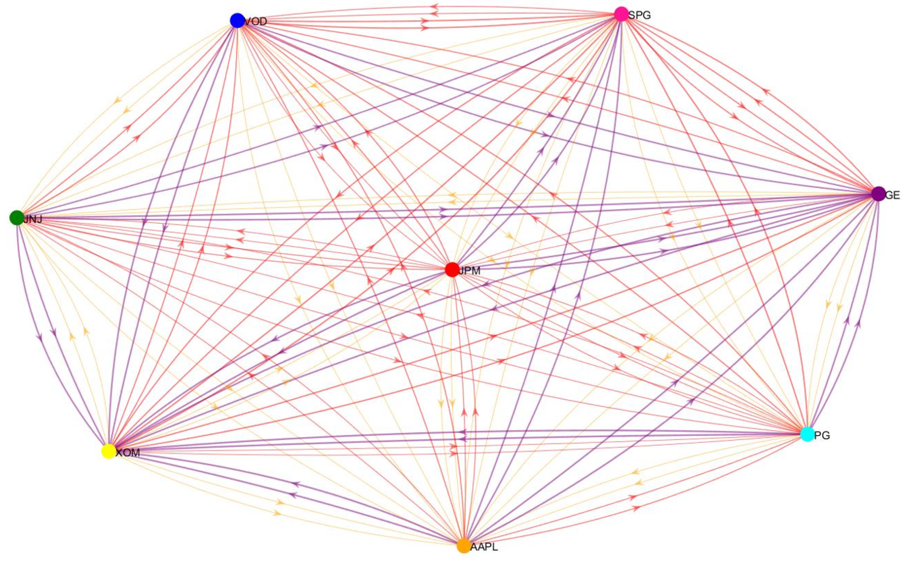
4.4. Complex Networks
5. Conclusions
- All of the selected typical stocks in U.S. industry sectors (except for JPM) exhibit long-range correlations and multifractal cross-correlations with JPM.
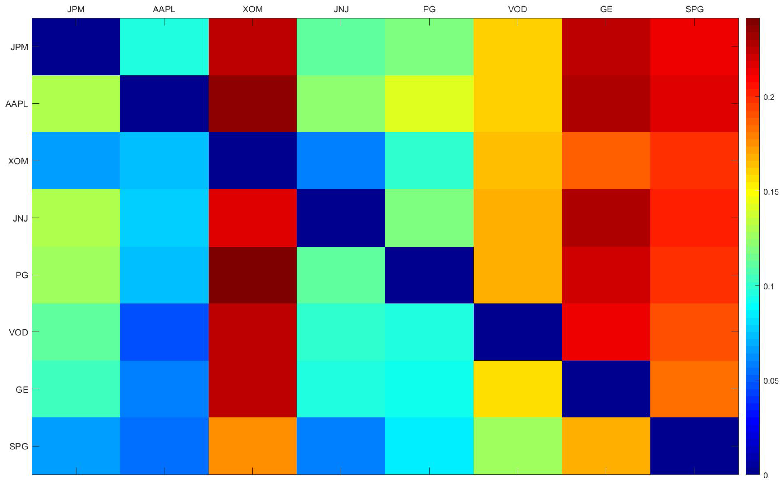
- The multifractal cross-correlation between JPM and XOM is the strongest, which implies that price volatility may have self-similarity and long memory characteristics at different time scales, i.e. there may be some degree of self-similarity and volatility aggregation characteristics in their price change patterns over a specific time horizon. During upswings in the economic cycle, increased demand for energy drives up oil prices and the earnings of energy firms, while economic expansion also tends to drive financial market activity and boost bank performance. Conversely, during economic downturns, falling energy demand and weakening financial activity can occur in tandem. Thus, the linkage effects between the financial and energy sectors are strong, making the multifractal cross-correlation between the two significant.
- The multifractal cross-correlation between JPM and VOD, as well as JPM and GE, is also strong. Volatility in the financial market and changes in interest rates affect VOD’s share price through, for example, the cost of funds. Both JPM and VOD are multinational companies, and in the context of globalization, complex multifractal characteristics are often reflected in the share price series of JPM and VOD, which implies that there is some self-similarity in the volatility behaviour of the two on different time scales in the short and long term and that when the market is volatile, the share prices of the two exhibit synchronicity.On the other hand, GE’s business covers a wide range of sectors, including aerospace, energy, and medical devices, which are closely related to the economic cycle and capital expenditures. When the economy is on the upswing, corporate capex increases, driving GE’s growth, while demand for loans and investments in the financial sector increases, positively affecting JPM. During economic downturns, capital expenditures decline, and demand for energy and industrial equipment weakens, affecting GE’s performance, reducing loan demand, increasing risk, and negatively impacting JPM. The similarity between the two over the economic cycle enhances their multiple fractal cross-correlation.
- From the perspective of information inflow analysis, the primary information source stocks for each stock are as follows:JNJ→JPM,JPM→AAPL,PG→XOM, AAPL→JNJ, AAPL→PG,PG→VOD,JNJ→GE, AAPL→SPG.From the perspective of information outflow analysis, the maximum information outflows for typical stocks in each industry sector are as follows: JPM → XOM, AAPL → XOM, XOM → SPG, JNJ → GE, PG → XOM, VOD → XOM, GE → XOM, SPG → XOM.
- In the complex network where the transfer entropy matrix is the adjacency matrix, AAPL has the highest , indicating that AAPL strongly influences other stocks. AAPL’s market performance and strategic decisions can significantly impact other companies’ stock prices and trends, reflecting its leadership position within the technology sector. Conversely, XOM has the highest , which indicates that XOM is more reliant on the influences of other industries, suggesting that the energy sector is driven to some extent by fluctuations in other sectors. Furthermore, XOM and GE have the highest WD, indicating that these two companies play important intermediary roles within the overall network, potentially facilitating the transmission of information and influence across multiple industries.
Author Contributions
Funding
Data Availability Statement
Acknowledgments
Conflicts of Interest
References
- Fama, E. F.; French, K. R. Business conditions and expected returns on stocks and bonds. Journal of Financial Economics 1989, 25(1), 23–49. [Google Scholar] [CrossRef]
- Bekaert, G.; Harvey, C. R. Foreign speculators and emerging equity markets. The Journal of Finance 2000, 55(2), 565–613. [Google Scholar] [CrossRef]
- Lehkonen, H. Stock market integration and the global financial crisis. Review of Finance 2015, 19(5), 2039–2094. [Google Scholar] [CrossRef]
- Borio, C.; Zhu, H. Capital regulation, risk-taking and monetary policy: a missing link in the transmission mechanism? Journal of Financial Stability 2012, 8(4), 236–251. [Google Scholar] [CrossRef]
- Chen, N. F.; Roll, R.; & Ross, S. A. Economic forces and the stock market. Journal of Business 1986, 383–403.
- Fama, E. F.; French, K. R. Industry costs of equity. Journal of Financial Economics 1997, 43(5), 153–193. [Google Scholar] [CrossRef]
- Kang, J. K. Why is there a home bias? An analysis of foreign portfolio equity ownership in Japan. Journal of Financial Economics 1997, 46(1), 3–28. [Google Scholar] [CrossRef]
- Zou, K. H.; Tuncali, K.; Silverman, S. G. Correlation and simple linear regression. Radiology 2003, 227(3), 617–628. [Google Scholar] [CrossRef]
- Zhang, Z.; Zhang, Y.; Shen, D.; Zhang, W. The dynamic cross-correlations between mass media news, new media news, and stock returns. Complexity 2018, 2018(1), 7619494. [Google Scholar] [CrossRef]
- Shan, J.; Pappas, N. The relative impacts of Japanese and US interest rates on local interest rates in Australia and Singapore. Applied Financial Economics 2000, 10, 291–298. [Google Scholar] [CrossRef]
- Dionisio, A.; Menezes, R.; Mendes, D. A. Mutual information: a measure of dependency for nonlinear time series. Physica A 2004, 344, 326–329. [Google Scholar] [CrossRef]
- Abigail, J. A complex network model for seismicity based on mutual information. Physica A 2013, 392, 2498–2506. [Google Scholar]
- Fiedor, P. Networks in financial markets based on the mutual information rate. Physical Review E 2014, 89, 052801. [Google Scholar] [CrossRef] [PubMed]
- Bland, J. M.; Altman, D. G. Statistical methods for assessing agreement between two methods of clinical measurement. The Lancet 1986, 327(8476), 307–310. [Google Scholar] [CrossRef]
- Ghysels, E.; Hill, J. B.; Motegi, K. Testing for Granger causality with mixed frequency data. Journal of Econometrics 2016, 192, 207–230. [Google Scholar] [CrossRef]
- Shojaie, A.; Fox, E. B. Granger causality: A review and recent advances. Ann. Rev. Stat. Appl. 2022, 9(1), 289–319. [Google Scholar] [CrossRef]
- Dionisio, A.; Menezes, R.; Mendes, D. A. Mutual information: a measure of dependency for nonlinear time series. Physica A: Statistical Mechanics and its Applications 2004, 344(1-2). 326–329. [CrossRef]
- Pan, Y.; Hou, L.; Pan, X. Interplay between stock trading volume, policy, and investor sentiment: A multifractal approach. Physica A: Statistical Mechanics and its Applications 2022, 603, 127706. [Google Scholar] [CrossRef]
- Peng, C.-K.; Buldyrev, S. V.; Havlin, S.; Simons, M.; Stanley, H. E.; Goldberger, A. L. Mosaic organization of DNA nucleotides. Physical Review E 1994, 49, 1685–1689. [Google Scholar] [CrossRef]
- Kantelhardt, J. W.; Zschiegner, S. A.; Koscielny-Bunde, E.; Havlin, S.; Bunde, A.; Stanley, H. E. Multifractal detrended fluctuation analysis of nonstationary time series. Physica A: Statistical Mechanics and its Applications 2002, 316, 87–114. [Google Scholar] [CrossRef]
- Podobnik, B.; Stanley, H. E. Detrended cross-correlation analysis: a new method for analyzing two nonstationary time series. Physical Review Letters 2008, 100, 84102. [Google Scholar] [CrossRef] [PubMed]
- Zhou, W.-X. Multifractal detrended cross-correlation analysis for two nonstationary signals. Physical Review E 2008, 77, 66211. [Google Scholar] [CrossRef] [PubMed]
- Shadkhoo, S.; Jafari, G. R. Multifractal detrended cross-correlation analysis of temporal and spatial seismic data. The European Physical Journal B 2009, 72, 679–683. [Google Scholar] [CrossRef]
- Zhuang, X.; Wei, Y.; Zhang, B. Multifractal detrended cross-correlation analysis of carbon and crude oil markets. Physica A: Statistical Mechanics and its Applications 2014, 399, 113–125. [Google Scholar] [CrossRef]
- Gong, X.; Jia, G. Z. Exploring the Cross-Correlations between Tesla Stock Price, New Energy Vehicles and Oil Prices: A Multifractal and Causality Analysis. Fluctuation and Noise Letters 2024, 2450024. [Google Scholar] [CrossRef]
- Ahmed, H.; Aslam, F.; Ferreira, P. Navigating Choppy Waters: Interplay between Financial Stress and Commodity Market Indices. Fractal and Fractional 2024, 8, 96. [Google Scholar] [CrossRef]
- Acikgoz, T.; Gokten, S.; Soylu, A.B. Multifractal Detrended Cross-Correlations between Green Bonds and Commodity Markets: An Exploration of the Complex Connections between Green Finance and Commodities from the Econophysics Perspective. Fractal and Fractional 2024, 8, 117. [Google Scholar] [CrossRef]
- Ma, J.; Wang, T.; Zhao, R. Quantifying cross-correlations between economic policy uncertainty and Bitcoin market: Evidence from multifractal analysis. Discrete Dyn. Nat. Soc. 2022, 2022, 1072836. [Google Scholar] [CrossRef]
- Zhao, X.; Shang, P.; Shi, W. Multifractal cross-correlation spectra analysis on Chinese stock markets. Physica A: Statistical Mechanics and Its Applications 2014, 402, 84–92. [Google Scholar] [CrossRef]
- Yin, Y.; Shang, P. Modified cross sample entropy and surrogate data analysis method for financial time series. Physica A: Statistical Mechanics and its Applications 2015, 433, 17–25. [Google Scholar] [CrossRef]
- Gu, D.; Huang, J. Multifractal detrended cross-correlation analysis of high-frequency stock series based on ensemble empirical mode decomposition. Fractals 2020, 28(02), 2050035. [Google Scholar] [CrossRef]
- Schreiber, T. Measuring information transfer. Phys. Rev. Lett. 2000, 85(2), 461. [Google Scholar] [CrossRef] [PubMed]
- Servadio, J. L.; Convertino, M. Optimal information networks: application for data-driven integrated health in populations. Sci. Adv. 2018, 4. [Google Scholar] [CrossRef]
- Tongal, H.; Sivakumar, B. Forecasting rainfall using transfer entropy coupled directed-weighted complex networks. Atmos. Res. 2021, 255. [Google Scholar] [CrossRef]
- Gao, Y.; Su, H.; Li, R.; Zhang, Y. Synchronous analysis of brain regions based on multi-scale permutation transfer entropy. Comput. Biol. Med. 2019, 109, 272–279. [Google Scholar] [CrossRef]
- Sandoval Jr, L. Structure of a global network of financial companies based on transfer entropy. Entropy 2014, 16(8), 4443–4482. [Google Scholar] [CrossRef]
- Wang, X.; Gao, X.; Wu, T.; Sun, X. Dynamic multiscale analysis of causality among mining stock prices. Resources Policy 2022, 77, 102708. [Google Scholar] [CrossRef]
- Lempel, A.; Ziv, J. On the complexity of finite sequences. IEEE Trans. Inf. Theory 1976, 22, 75–81. [Google Scholar] [CrossRef]
- Costa, M.; et al. A study on the properties of complex systems. Phys. Rev. Lett. 2002, 89, 068102. [Google Scholar] [CrossRef]
- Gao, Z. K.; et al. Analysis of chemical engineering processes. Chem. Eng. J. 2016, 291, 74. [Google Scholar] [CrossRef]
- Marwan, N.; et al. Recurrence plots for the analysis of complex systems. Phys. Rep. 2007, 438, 237. [Google Scholar] [CrossRef]
- Albert, R.; Barabási, A. L. Statistical mechanics of complex networks. Rev. Mod. Phys. 2002, 74(1), 47. [Google Scholar] [CrossRef]
- Watts, D. J.; Strogatz, S. H. Collective dynamics of ‘small-world’ networks. Nature 1998, 393(6684), 440–442. [Google Scholar] [CrossRef] [PubMed]
- Barabási, A. L.; Albert, R. Emergence of scaling in random networks. Science 1999, 286(5439), 509–512. [Google Scholar] [CrossRef]
- Newman, M. E. Properties of highly clustered networks. Phys. Rev. E 2003, 68(2), 026121. [Google Scholar] [CrossRef] [PubMed]
- Dorogovtsev, S. N.; Goltsev, A. V.; Mendes, J. F. Critical phenomena in complex networks. Rev. Mod. Phys. 2008, 80(4), 1275–1335. [Google Scholar] [CrossRef]
- Albert, R.; Barabási, A. L. Statistical mechanics of complex networks. Rev. Mod. Phys. 2002, 74(1), 47–97. [Google Scholar] [CrossRef]
- Zhang, J.; Small, M. Complex network from pseudoperiodic time series: Topology versus dynamics. Phys. Rev. Lett. 2006, 96(23), 238701. [Google Scholar] [CrossRef]
- Sun, X.; Small, M.; Zhao, Y. et al. Characterizing system dynamics with a weighted and directed network constructed from time series data. Chaos 2014, 24(2), 024402. [Google Scholar] [CrossRef]
- Oh, G.; Oh, T.; Kim, H.; Kwon, O. An information flow among industry sectors in the Korean stock market. Journal of the Korean Physical Society 2014, 65, 2140–2146. [Google Scholar] [CrossRef]
- Wu, Z.; Huang, N.E. Ensemble empirical mode decomposition: A noise-assisted data analysis method. Adv. Adapt. Data Anal. 2009, 1, 1–41. [Google Scholar] [CrossRef]
- Podobnik, B.; Jiang, Z.Q.; Zhou, W.X.; Stanley, H.E. Statistical tests for power-law cross-correlated processes. Phys. Rev. E 2011, 84, 066118. [Google Scholar] [CrossRef] [PubMed]
- Zou, S.; Zhang, T. Multifractal Detrended Cross-Correlation Analysis of the Relation between Price and Volume in European Carbon Futures Markets. Phys. A Stat. Mech. Its Appl. 2020, 537, 122310. [Google Scholar] [CrossRef]
- Shannon, C. E. A mathematical theory of communication. The Bell System Technical Journal 1948, 27(3), 379–423. [Google Scholar] [CrossRef]
- Pluim, J. P.; Maintz, J. A.; Viergever, M. A. Mutual-information-based registration of medical images: a survey. IEEE Transactions on Medical Imaging 2003, 22(8), 986–1004. [Google Scholar] [CrossRef]
- Kraskov, A.; Stögbauer, H.; Grassberger, P. Estimating mutual information. Physical Review E 2004, 69, 066138. [Google Scholar] [CrossRef]
- Grassberger, P. Physical Review Letters 1985, 107A, 101.
- Somorjai, R. L. Methods for Estimating the Intrinsic Dimensionality of High-Dimensional Point Sets. In Dimensions and Entropies in Chaotic Systems; Mayer-Kress, G., Ed.; Springer: Berlin, 1986.
- Kozachenko, L. F.; Leonenko, N. N. Problems of Information Transmission 1987, 23, 95.
- Lee, J. , Nemati, S., Silva, I., Edwards, B. A., Butler, J. P., & Malhotra, A. Transfer entropy estimation and directional coupling change detection in biomedical time series. Biomedical Engineering Online 2012, 11, 1–17. [Google Scholar]
- Neto, D. Examining interconnectedness between media attention and cryptocurrency markets: A transfer entropy story. Economics Letters 2022, 214, 110460. [Google Scholar] [CrossRef]
- Bekiros, S. , Nguyen, D.K., Junior, L.S., Uddin, G.S. Information diffusion, cluster formation and entropy-based network dynamics in equity and commodity markets. European Journal of Operational Research 2017, 256. [Google Scholar] [CrossRef]
- Kaiser, A. , Schreiber, T. Information transfer in continuous processes. Physica D: Nonlinear Phenomena 2002, 166, 43–62. [Google Scholar] [CrossRef]
- Unicomb, S.; Iñiguez, G.; Karsai, M. Threshold driven contagion on weighted networks. Scientific Reports 2018, 8(1), 3094. [Google Scholar] [CrossRef] [PubMed]
- Albert, R.; Barabási, A. L. Statistical mechanics of complex networks. Rev. Mod. Phys. 2002, 74(1), 47–97. [Google Scholar] [CrossRef]
- He, J.; Shang, P. Comparison of transfer entropy methods for financial time series. Phys. A Stat. Mech. Appl. 2017, 482, 772–785. [Google Scholar] [CrossRef]
- Wang, M. Analyzing the non-linearity of Chinese stock market using R/S method. Forecasting 2002, 21, 42–45. [Google Scholar]
- Li, Y.; Vilela, A.L.M.; Stanley, H.E. The institutional characteristics of multifractal spectrum of China’s stock market. Phys. Stat. Mech. Appl. 2020, 550. [Google Scholar] [CrossRef]
- Wu, Z.; Huang, N.E. Ensemble empirical mode decomposition: A noise-assisted data analysis method. Adv. Adapt. Data Anal. 2009, 1, 1–41. [Google Scholar] [CrossRef]
- Zebende, G.F. DCCA Cross-Correlation Coefficient: Quantifying Level of Cross-Correlation. Phys. A Stat. Mech. Its Appl. 2011, 390, 614–618. [Google Scholar] [CrossRef]
- Podobnik, B.; Jiang, Z. Q.; Zhou, W. X.; Stanley, H. E. Statistical tests for power-law cross-correlated processes. Physical Review E—Statistical, Nonlinear, and Soft Matter Physics 2011, 84(6), 066118. [Google Scholar] [CrossRef]
- Rizvi, S. A. R.; Dewandaru, G.; Bacha, O. I.; Masih, M. An analysis of stock market efficiency: Developed vs Islamic stock markets using MF-DFA. Physica A: Statistical Mechanics and its Applications 2014, 407, 86–99. [Google Scholar] [CrossRef]
- Kantelhardt, J. W.; Koscielny-Bunde, E.; Rego, H. H.; Havlin, S.; Bunde, A. Detecting long-range correlations with detrended fluctuation analysis. Physica A: Statistical Mechanics and its Applications 2001, 295(3-4). 441–454. [CrossRef]
- Hu, K.; Ivanov, P. C.; Chen, Z.; Carpena, P.; Stanley, H. E. Effect of trends on detrended fluctuation analysis. Physical Review E 2001, 64(1), 011114. [Google Scholar] [CrossRef] [PubMed]
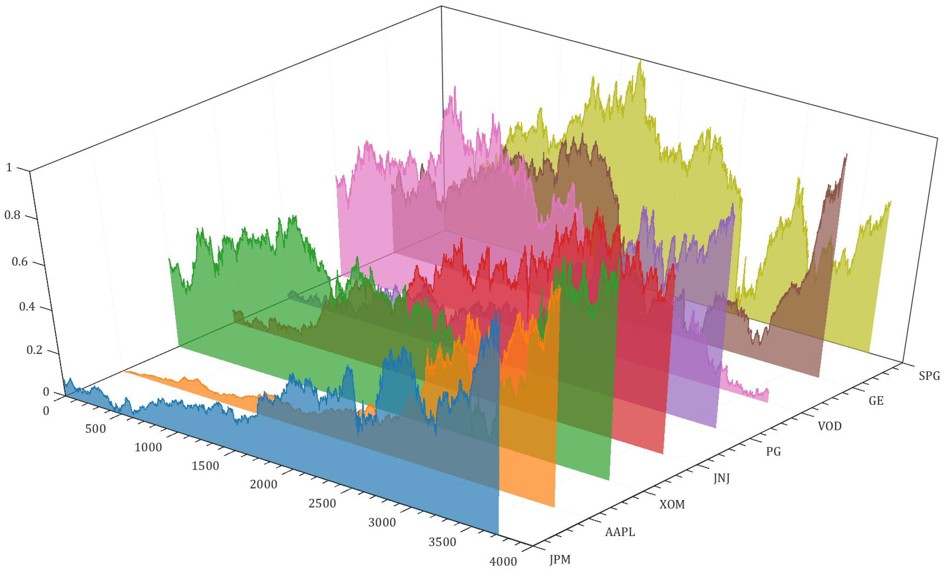

| Ticker Symbol | Listed Company | Industry Sector |
|---|---|---|
| IPM | JPMorgan Chase & Co. | Financial |
| AAPL | Apple Inc. | Technology |
| XOM | Exxon Mobil Corporation | Energy |
| JNJ | Johnson & Johnson | Healthcare |
| PG | Procter & Gamble Co. | Consumer staples |
| VOD | Vodafone Group Plc | Telecommunications |
| GE | General Electric Company | Manufacturing |
| SPG | Simon Property Group, Inc. | Real estate |
| JPM | AAPL | XOM | JNJ | PG | VOD | GE | SPG | |
|---|---|---|---|---|---|---|---|---|
| Min | 28.38 | 6.86 | 31.45 | 57.02 | 58.51 | 8.06 | 27.36 | 44.01 |
| Max | 224.80 | 234.82 | 125.37 | 186.01 | 177.79 | 41.57 | 192.63 | 227.60 |
| Mean | 92.22 | 67.33 | 82.15 | 118.82 | 100.79 | 23.55 | 92.53 | 141.62 |
| Std | 46.00 | 62.54 | 17.89 | 37.16 | 33.44 | 8.47 | 36.40 | 37.27 |
| Skewness | 0.61 | 0.99 | -0.35 | -0.16 | 0.60 | -0.18 | 0.23 | -0.32 |
| Kurtosis | -0.50 | -0.50 | 0.28 | -1.25 | -1.09 | -1.07 | -0.93 | -0.55 |
| JB_test | 273.17*** | 645.79*** | 87.30*** | 260.37*** | 403.89*** | 195.62*** | 165.70*** | 109.04*** |
| Probability | 4.80e-60 | 5.87e-141 | 1.10e-19 | 2.90e-57 | 1.98e-88 | 3.32e-43 | 1.04e-36 | 2.10e-24 |
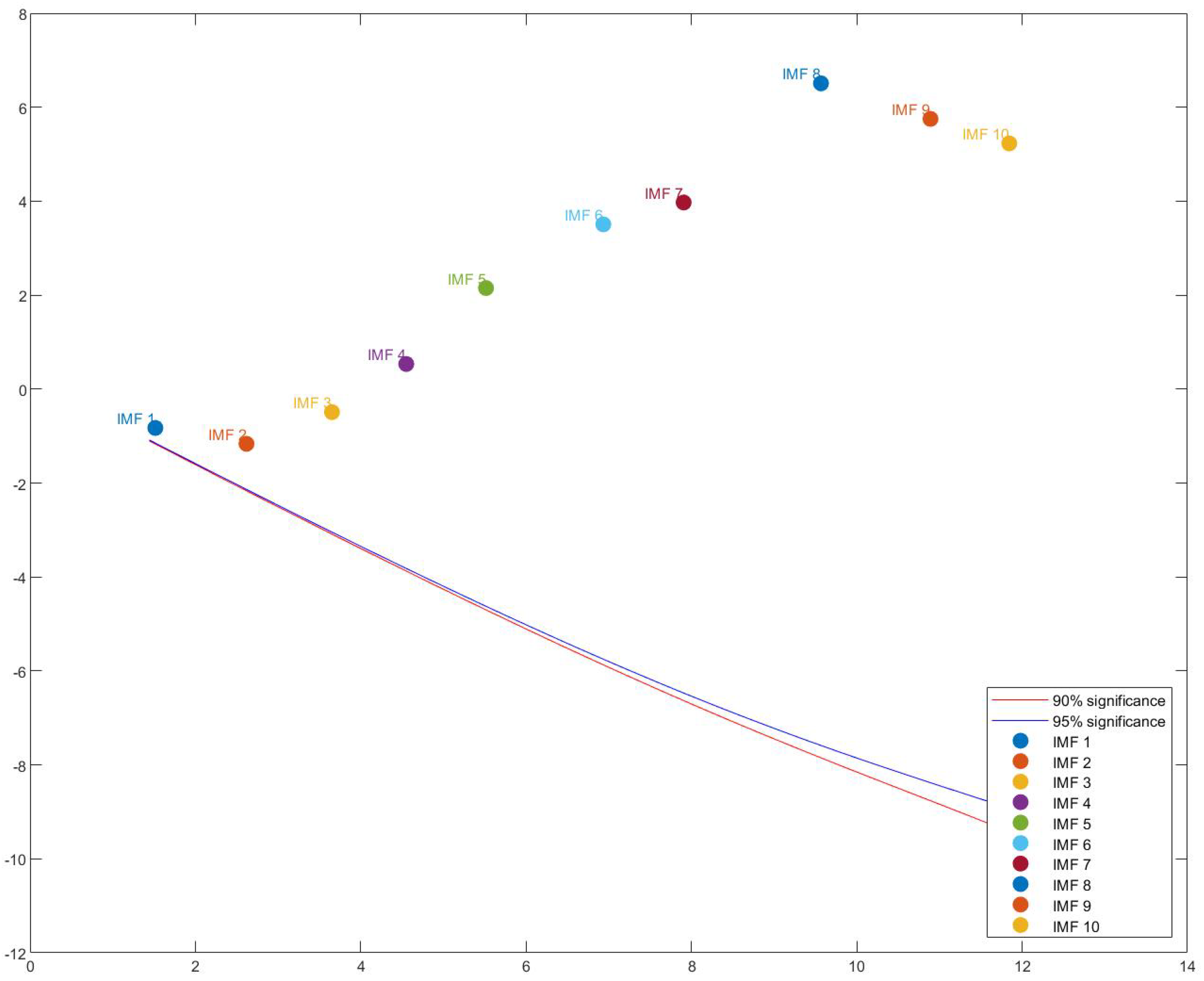
| IMF/Res | Pearson Corr | Kendall Corr | lnE | lnT | Var Contrib |
|---|---|---|---|---|---|
| IMF 1 | 0.0166 | 0.0063 | -0.8273 | 1.5179 | 0.0001 |
| IMF 2 | 0.0193 | 0.0181 | -1.1965 | 2.5665 | 0.0001 |
| IMF 3 | 0.0210 | 0.0074 | -0.4544 | 3.6371 | 0.0002 |
| IMF 4 | 0.0399 | 0.0110 | 0.5349 | 4.7042 | 0.0004 |
| IMF 5 | 0.0180 | 0.0005 | 2.1469 | 5.8911 | 0.0011 |
| IMF 6 | 0.1460 | 0.0380 | 3.5085 | 6.9376 | 0.0029 |
| IMF 7 | -0.0239 | 0.0096 | 3.9466 | 6.2160 | 0.0040 |
| IMF 8 | -0.3526 | -0.0577 | 6.5376 | 9.5644 | 0.0230 |
| IMF 9 | 0.3714 | 0.1371 | 5.7326 | 10.8955 | 0.0124 |
| IMF 10 | -0.3299 | -0.3498 | 5.2111 | 11.8322 | 0.0081 |
| Residual | 0.9750 | 0.8128 | N/A | N/A | 1.1231 |
| JPM | AAPL | XOM | JNJ | PG | VOD | GE | SPG | |
|---|---|---|---|---|---|---|---|---|
| JPM | 0 | 0.0977 | 0.2264 | 0.1100 | 0.1206 | 0.1619 | 0.2254 | 0.2149 |
| AAPL | 0.1292 | 0 | 0.2363 | 0.1231 | 0.1430 | 0.1606 | 0.2277 | 0.2155 |
| XOM | 0.0667 | 0.0729 | 0 | 0.0574 | 0.1011 | 0.1627 | 0.1850 | 0.1980 |
| JNJ | 0.1306 | 0.0770 | 0.2184 | 0 | 0.1200 | 0.1663 | 0.2288 | 0.2019 |
| PG | 0.1251 | 0.0748 | 0.2415 | 0.1118 | 0 | 0.1676 | 0.2196 | 0.1981 |
| VOD | 0.1118 | 0.0489 | 0.2229 | 0.0995 | 0.0960 | 0 | 0.2130 | 0.1922 |
| GE | 0.1038 | 0.0582 | 0.2255 | 0.0951 | 0.0943 | 0.1560 | 0 | 0.1827 |
| SPG | 0.0678 | 0.0544 | 0.1749 | 0.0570 | 0.0862 | 0.1271 | 0.1674 | 0 |
| WD | NTE | WCC | |||
|---|---|---|---|---|---|
| JPM | 1.1569 | 0.7351 | 1.8919 | 0.4218 | 0.1490 |
| AAPL | 1.2348 | 0.4838 | 1.7187 | 0.7510 | 0.1532 |
| XOM | 0.8439 | 1.5458 | 2.3898 | -0.7019 | 0.1372 |
| JNJ | 1.1429 | 0.6540 | 1.7969 | 0.4889 | 0.1513 |
| PG | 1.1383 | 0.7611 | 1.8995 | 0.3772 | 0.1489 |
| VOD | 0.9843 | 1.1021 | 2.0864 | -0.1179 | 0.1444 |
| GE | 0.9155 | 1.4662 | 2.3817 | -0.5506 | 0.1374 |
| SPG | 0.7348 | 1.4034 | 2.1382 | -0.6685 | 0.1432 |
Disclaimer/Publisher’s Note: The statements, opinions and data contained in all publications are solely those of the individual author(s) and contributor(s) and not of MDPI and/or the editor(s). MDPI and/or the editor(s) disclaim responsibility for any injury to people or property resulting from any ideas, methods, instructions or products referred to in the content. |
© 2024 by the authors. Licensee MDPI, Basel, Switzerland. This article is an open access article distributed under the terms and conditions of the Creative Commons Attribution (CC BY) license (http://creativecommons.org/licenses/by/4.0/).


