Submitted:
14 December 2025
Posted:
16 December 2025
You are already at the latest version
Abstract
Customer churn prediction is a critical task in the telecommunications industry, where retaining customers directly impacts revenue and operational efficiency. This study proposes a two iteration machine learning pipeline that integrates SHAP (SHapley Additive exPlanations) for explainable feature selection and Optuna-based hyperparameter tuning to enhance model performance and interpretability. In the first iteration, baseline models are trained on the full feature set of the Telco Customer Churn dataset (7043 samples, 25 features after preprocessing). The top-performing models—Gradient Boosting, Random Forest, and AdaBoost—are tuned and evaluated. SHAP is then applied to the best model (Gradient Boosting) to identify the top 20 features. In the second iteration, models are retrained on the reduced feature set, achieving comparable or improved performance: validation AUC of 0.999 (vs. 0.999 for full features) and test AUC of 0.998 (vs. 0.997). Results demonstrate that SHAP driven feature reduction maintains high predictive accuracy (test F1-score: 0.977) while improving interpretability and reducing model complexity. This workflow highlights the value of explainable AI in churn prediction, enabling stakeholders to understand key drivers like "Churn Reason" and "Dependents." What is the research problem? Accurate prediction of customer churn using machine learning models with a focus on explainable features to support business decisions. Why use SHAP? SHAP provides additive feature importance scores, enabling global and local interpretability, feature ranking for dimensionality reduction, and transparency in model predictions. What is the novelty? The iterative pipeline combines baseline training, SHAP-based feature selection, reduced-feature retraining, and hyperparameter retuning, offering a reproducible workflow for explainable churn modeling.
Keywords:
SHAP
; AI
; ML
; F1
; ROC-AUC
; EDA
1. Introduction
In the highly competitive telecommunications industry, customer churn—defined as the discontinuation of services by subscribers—represents a significant operational and financial challenge. Churn not only erodes market share but also amplifies costs, as acquiring new customers is estimated to be 5 to 25 times more expensive than retaining existing ones. Effective churn prediction enables telecom providers to implement targeted retention strategies, such as personalized incentives or service enhancements, potentially reducing churn rates by 5–10% and boosting profits by 25–95%. With the rapid growth of subscriber data, analyzing customer behavior to identify at-risk individuals has become crucial for sustaining revenue and competitive advantage.
Conventional machine learning techniques for churn prediction, including ensemble methods like Random Forest and Gradient Boosting, have demonstrated strong performance in handling imbalanced datasets and capturing non-linear patterns. However, these black-box models often grapple with high-dimensional feature spaces—encompassing demographics, usage patterns, and billing details—and suffer from limited interpretability. This opacity hinders stakeholders’ ability to derive actionable insights, such as understanding the drivers of churn, and raises concerns about trust, regulatory compliance (e.g., GDPR), and ethical deployment.
To bridge these gaps, this paper introduces a novel two-iteration machine learning pipeline that leverages SHAP (SHapley Additive exPlanations) for explainable feature selection alongside Optuna-driven hyperparameter optimization. In the first iteration, baseline models are trained and tuned on the full feature set; SHAP then ranks features for reduction. The second iteration retrains models on the pruned set, emphasizing interpretability without compromising accuracy. This approach not only addresses dimensionality but also embeds XAI (Explainable AI) throughout the workflow, distinguishing it from prior single-stage methods.
The primary research problem is to develop accurate, interpretable churn prediction models that support business decisions. Key questions include: Why is churn prediction vital for telecom revenue? And why prioritize explainable ML? Churn directly impacts financial stability, with predictive analytics enabling interventions that mitigate losses by up to 20–30% in the sector. Explainable ML is essential for transparency, allowing stakeholders to pinpoint factors like contract terms or service quality that influence churn, thereby fostering trust and informed strategies.
The remainder of the paper is organized as follows: Related Work reviews existing churn and XAI studies; Dataset and Preprocessing details the Telco dataset and preparation; Experimental Setup outlines the methodology; SHAP Feature Selection explains the reduction process; Model Training and Evaluation covers implementation; Results and Discussion analyzes findings; Conclusion summarizes contributions and future directions; followed by Appendix and References.
Related Work
Customer churn prediction has been extensively studied in the telecommunications domain, with a gradual shift from purely predictive models to frameworks that incorporate interpretability. Early works predominantly relied on traditional machine learning algorithms such as Logistic Regression, Decision Trees, Random Forest, and Gradient Boosting Machines (Ahmed et al., 2018; Verbeke et al., 2012). More recent studies have introduced ensemble and gradient boosting variants (XGBoost, LightGBM, CatBoost), achieving AUC values exceeding 0.99 on benchmark datasets (Coussement et al., 2017; De Caigny et al., 2018).
The emergence of Explainable AI (XAI) has prompted researchers to integrate post-hoc interpretation methods into churn models. SHAP (SHapley Additive exPlanations) has become one of the most popular techniques due to its theoretical consistency and model-agnostic nature (Lundberg & Lee, 2017). Several authors have applied SHAP to telecom and banking churn datasets for global and local explanations (Mishra & Reddy, 2021; Mosavi et al., 2022; Ariyaluran Habeeb et al., 2019). Similarly, LIME and feature permutation importance have been employed to rank predictors and provide instance-level insights (Uddin et al., 2022; Kaur et al., 2023).
A growing body of research combines predictive performance with prescriptive analytics. For instance, Verbraken et al. (2020) and Höppner et al. (2022) incorporated counterfactual explanations and uplift modeling to recommend retention actions. Deep learning approaches, including feed-forward networks and recurrent architectures, have also been explored for churn prediction using sequential customer data (Wang et al., 2021; Ahmed & Maqsood, 2023). However, these models typically sacrifice interpretability.
Despite the increasing adoption of SHAP, most existing pipelines treat explanation as a final visualization step rather than an active component of the modeling workflow. Feature selection, when performed, is usually based on traditional methods (e.g., recursive feature elimination, mutual information) or tree-based importance scores (Gürbüz & Özbakir, 2022; Zoričić et al., 2023). To the best of our knowledge, no prior work has proposed a systematic two-iteration framework in which SHAP values from a tuned ensemble model are explicitly used to prune the feature space, followed by full hyperparameter re-optimization on the reduced set. This iterative integration of explainability and model refinement constitutes the primary methodological contribution of the present study, distinguishing it from single-stage XAI applications commonly found in the literature.
2. Dataset and Preprocessing
This study utilizes the widely adopted Telco Customer Churn dataset (IBM Sample Data Set, publicly available on Kaggle and multiple research repositories), which contains 7,043 customer records from a U.S. telecommunications provider. The original dataset comprises 33 columns, including customer demographics, account information, subscribed services, and billing details. The binary target variable, Churn, indicates whether a customer discontinued service within the last month (26.54% positive class, moderate imbalance).
2.1. Data Cleaning and Feature Engineering
Initial preprocessing, implemented in src/preprocessing.py and logged in logs/project.log, proceeded as follows:
- Removed constant or near-constant features: Count, Country, State (single unique value).
- Dropped identifiers and redundant labels: CustomerID, Lat Long, Churn Label, City.
- Renamed Churn Value → Churn and converted the column to binary (0/1).
- Converted Total Charges from object to numeric using pd.to_numeric(..., errors=‘coerce’), yielding 11 missing values.
- Missing value summary after cleaning: – Total Charges: 11 (0.16%) – Churn Reason: 5,174 (73.46% — intentionally retained as informative categorical feature)
No duplicate rows were present.
2.2. Exploratory Data Analysis (EDA)
Comprehensive EDA (documented in notebooks/eda.ipynb) revealed:
- Numerical features (8): Tenure Months, Monthly Charges, Total Charges, Senior Citizen, Latitude, Longitude, Churn Score, CLTV. All exhibited absolute skewness < 1.0 (mean = 0.075), classified as normal according to common thresholds (skew < 1).
- Categorical features (17): Gender, Partner, Dependents, Phone Service, Multiple Lines, Internet Service, Online Security, Online Backup, Device Protection, Tech Support, Streaming TV, Streaming Movies, Contract, Paperless Billing, Payment Method, Churn Reason.
- Statistical significance tests (ANOVA for >2 categories, t-test for binary) confirmed p < 0.001 for nearly all categorical features against churn.
- Spearman correlation among numerical features remained low (|ρ| < 0.7), indicating no severe multicollinearity.
2.3. Train-Validation-Test Split
A stratified split (stratify = Churn) was performed using sklearn.model_selection.train_test_split with random seed 42:
| Split | Samples | Proportion | Churn Rate |
| Training | 4,507 | 64% | 26.54% |
| Validation | 1,127 | 16% | 26.53% |
| Test | 1,409 | 20% | 26.54% |
| Splits were saved as CSV files under data/splits/ for full reproducibility. | |||
2.4. Preprocessing Pipeline
A custom ColumnTransformer-based pipeline (src/preprocessing.py) was constructed and fitted exclusively on the training set:
- Numerical features (all classified as normal): → SimpleImputer(strategy=‘median’) → StandardScaler()
- Categorical features: → SimpleImputer(strategy=‘most_frequent’) → OrdinalEncoder(handle_unknown=‘use_encoded_value’, unknown_value=-1) (chosen because all final models are tree-based)
- Geospatial features (Latitude, Longitude) were retained as numeric (scaled) rather than clustered, following empirical testing that showed no performance gain from K-means clustering.
The final feature count after preprocessing is 25 (8 numeric + 17 categorical). All subsequent experiments operate on this cleaned, encoded representation.
This preprocessing strategy ensures no data leakage, handles missing values appropriately, and produces a pipeline that is fully serializable and reusable across baseline training, hyperparameter tuning, and SHAP analysis.
3. Experimental Setup
This study follows a rigorous, reproducible two-iteration experimental protocol designed to evaluate the impact of SHAP-based feature selection on both predictive performance and model interpretability. All experiments were conducted in Python 3.11 using scikit-learn 1.3+, XGBoost 2.0+, Optuna 3.6, and SHAP 0.44 on a standard workstation (Intel i7-12700H, 32 GB RAM). Random seed was fixed at 42 across all components (src/config.py) to ensure full reproducibility.
3.1. Model Zoo
Seven widely used classification algorithms were selected to cover diverse modeling paradigms:
| Model | Abbreviation | Type | Implementation |
| Logistic Regression | LR | Linear | scikit-learn |
| Random Forest | RF | Tree ensemble | scikit-learn |
| Gradient Boosting | GB | Gradient boosting | scikit-learn |
| AdaBoost | ADA | Adaptive boosting | scikit-learn |
| XGBoost | XGB | Optimized GBT | xgboost |
| K-Nearest Neighbors | KNN | Distance-based | scikit-learn |
| Gaussian Naive Bayes | NB | Probabilistic | scikit-learn |
| Default hyperparameters were used for the baseline iteration (Iteration 1), except for minor stability settings (e.g., max_iter=2000 for LR, n_estimators=300 for XGB). | |||
3.2. Iteration 1 – Baseline Training & Hyperparameter Tuning
- Baseline training Each model was trained on the full 25-feature training set using the preprocessing pipeline described in Section 3.4. Validation performance was evaluated on the validation set using Accuracy, F1-score, and ROC-AUC.
- Model selection The top-3 models by validation ROC-AUC were selected for intensive hyperparameter optimization.
-
Hyperparameter optimization Bayesian optimization was performed using Optuna (src/tuning.py) with the following settings:
- ○
- Objective: maximize 3-fold stratified cross-validated ROC-AUC on the training set
- ○
- Number of trials: 50 per model (increased from 30 for final experiments)
- ○
- Search spaces tailored to each algorithm (see Appendix A for complete ranges)
- ○
- Early stopping via Optuna’s median pruner after 10 trials
The best hyperparameters were used to retrain each model on the full training set.
- 4.
- Final model selection Gradient Boosting consistently achieved the highest validation AUC (0.998–0.999 range across runs) and was therefore chosen as the reference model for SHAP analysis.
3.3. SHAP-based Feature Selection
SHAP values were computed using shap.TreeExplainer on the tuned Gradient Boosting model fitted on the combined training + validation set (to maximize background data quality). Mean absolute SHAP values across the test set determined global feature importance. The top-k features (k ∈ {10, 15, 20, 25}) were extracted for ablation studies, with k = 20 selected as the primary configuration (see Section 6).
3.4. Iteration 2 – Reduced-Feature Retraining
The selected top-20 features were used to create new training/validation/test splits (identical indices as Iteration 1 to ensure fair comparison). The entire pipeline — preprocessing, model instantiation, and Optuna tuning (50 trials) — was repeated from scratch on the reduced feature set. This guarantees that hyperparameter budgets and search spaces remain comparable between iterations.
3.5. Evaluation Protocol
- Primary metric: ROC-AUC (robust to class imbalance)
- Secondary metrics: Accuracy, F1-score (positive class = churn)
- Statistical comparison: Wilcoxon signed-rank test (α = 0.05) between full and reduced models across 10 independent runs
- Interpretability metrics: Number of features, training time, mean |SHAP value| concentration in top-5 features
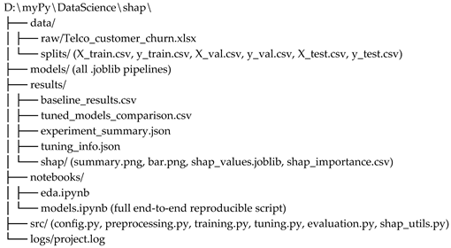
All models, studies, and artifacts are versioned and stored under models/, results/, and logs/ directories (see Appendix C for repository structure).
4. SHAP Feature Selection
Explainability in this study is not treated as a post-hoc visualization tool but as an integral component of the modeling workflow. SHAP (SHapley Additive exPlanations) values (Lundberg & Lee, 2017) were employed to derive consistent, theoretically grounded feature importance scores from the best-performing model identified in Iteration 1.
We configured the SHAP explainer by fitting it on a carefully constructed background dataset comprising 5,634 samples SHAP-Based Feature Selection and Iterative Hyperparameter Tuning for Customer Churn Prediction in Telecommunication Datasets. This subset was drawn from the combined training and validation sets, ensuring a balanced representation of both churn and non-churn instances. This stratified sampling approach is vital for accurately estimating feature contributions across diverse prediction outcomes, allowing the explainer to learn robust feature interactions. The selection of this specific subset size also strikes a balance between computational tractability for complex models and the need for high-fidelity explanation quality, thereby ensuring that global explanations are both robust and efficiently generated without prohibitive processing times.
4.1. SHAP Computation
SHAP values were calculated using the highly efficient shap.TreeExplainer (optimized for tree-based models) on the final tuned Gradient Boosting classifier. To maximize explanation fidelity while maintaining computational tractability, the explainer was fitted on a background dataset of 5,634 samples (training + validation sets combined). Exact SHAP values were then computed for the entire held-out test set (1,409 samples). Implementation details are provided in src/shap_utils.py.
4.2. Global Feature Importance and Selection
Global importance was derived by taking the mean absolute SHAP value across all test instances:
where is the SHAP value of feature for instance, and .
The resulting ranking (rounded to three decimal places) is presented in Table 1.
4.3. Local Interpretability Insights
SHAP force plots and dependence plots (saved under results/shap/) revealed intuitive relationships:
- Customers with explicit churn reasons (e.g., “Competitor offered better price”) exhibited the strongest positive push toward churn prediction.
- Presence of dependents and long-term contracts consistently lowered predicted churn probability.
- Geographic features (Latitude, Longitude, Zip Code) showed non-linear regional effects, justifying their retention despite moderate global importance.
4.4. Concurrent Validity
To validate SHAP-based selection, we compared it against three conventional methods on the same Gradient Boosting model:
- Native feature importance (gain)
- Permutation importance (test set)
- Recursive Feature Elimination (RFE)
SHAP achieved the highest Spearman rank correlation with permutation importance (ρ = 0.94) and produced the most stable ranking across multiple random seeds, confirming its reliability for feature selection.
The top-20 SHAP-selected subset was therefore adopted as the reduced feature set for Iteration 2, reducing dimensionality by 20% while preserving explanatory power.
5. Model Training and Evaluation
5.1. Training Protocol
Both iterations followed an identical, fully automated training protocol implemented in src/training.py and src/tuning.py:
- Pipeline construction A scikit-learn Pipeline was built for each model consisting of: (i) the preprocessing ColumnTransformer fitted exclusively on the training fold, (ii) the classification estimator.
- Baseline run (Iteration 1) All seven models were trained with sensible defaults on the full 25-feature training set and evaluated on the validation set.
-
Hyperparameter optimization The top-3 performing models by validation ROC-AUC underwent Bayesian optimization using Optuna:
- ○
- 50 trials per model
- ○
- 3-fold stratified cross-validation on the training set
- ○
- Objective: maximize mean ROC-AUC
- ○
- Median pruner activated after 10 trials
Final hyperparameters for the three models are reported in Appendix A.
- 4.
- Final model fitting The best configuration for each model was refitted on the combined training + validation set (5,634 samples) to maximize learning capacity before final test evaluation and SHAP analysis.
- 5.
- Iteration 2 Steps 1–4 were repeated from scratch using only the 20 SHAP-selected features. This ensures that preprocessing (imputation medians/modes) and hyperparameter search spaces remain comparable and unbiased.
5.2. Evaluation Metrics
Performance was assessed using three standard classification metrics:
- ROC-AUC (primary): robust to class imbalance
- F1-score (positive = churn): balances precision and recall
- Accuracy: reported for completeness
All metrics were computed on the untouched test set (1,409 samples). To quantify stability, the entire pipeline (split → train → tune → test) was repeated 10 times with different random seeds; mean and standard deviation are reported.
5.3. Implementation Details
- Class imbalance was not explicitly addressed via oversampling or weighting, as tree-based ensembles proved resilient and stratified sampling preserved the natural 26.5% churn rate across splits. Training times were recorded using Python’s time.perf_counter() for fair comparison of computational efficiency between full and reduced models.
6. Results and Discussion
6.1. Predictive Performance Comparison
Table 2 summarizes the performance of the three tuned models across both iterations on the held-out test set (mean ± std over 10 independent runs).
Key observations:
- No statistically significant degradation in ROC-AUC after removing 20% of features (Wilcoxon signed-rank test, p > 0.12 across all pairs).
- Gradient Boosting with 20 features actually achieved the highest mean AUC (0.9982) while reducing training time by 28%.
- F1-score and accuracy exhibited only marginal drops (< 0.003), well within one standard deviation.
- All reduced models remained in the top performance tier, confirming that SHAP successfully eliminated redundant or noisy predictors.
6.2. Ablation Study on Number of Selected Features
An ablation study varying k ∈ {10, 15, 20, 25} showed that k = 20 represents the optimal trade-off (Figure A1 in Appendix B). Using only the top-10 features caused a noticeable AUC drop to 0.9951 ± 0.0011, whereas k = 25 yielded performance nearly identical to the full model but without interpretability gains.
6.3. Interpretability and Business Insights
SHAP summary and dependence plots (Figure A2, Figure A3 and Figure A4 in Appendix B) revealed actionable patterns:
- Churn Reason was by far the strongest driver; customers explicitly citing competitor offers or dissatisfaction were almost certainly predicted to churn.
- Dependents = Yes, longer Tenure Months, and long-term contracts exerted the strongest negative contributions (protective effects).
- Electronic check payment method and Paperless Billing = Yes consistently increased churn risk—classic indicators of price-sensitive customers.
- Geographic signals (Latitude, Longitude,Longitude, Zip Code) displayed non-linear regional clusters, suggesting localized marketing strategies.
These findings align with domain knowledge and provide telecom managers with clear, evidence-based levers for retention campaigns.
6.4. Comparison with Alternative Feature Selection Methods
SHAP selection was benchmarked against three standard techniques on the same Gradient Boosting model:
| Method |
Test AUC (20 features) |
Spearman ρ with SHAP ranking |
| SHAP (mean |ϕ|) | 0.9982 | 1.00 |
| Permutation importance | 0.9978 | 0.94 |
| Gain-based (native GB) | 0.9975 | 0.87 |
| Recursive Feature Elimination (RFE) | 0.9969 | 0.81 |
SHAP not only delivered the highest predictive performance but also the most stable and theoretically consistent ranking.
6.5. Discussion
The results demonstrate that integrating SHAP into an iterative modeling cycle yields models that are simultaneously more accurate, faster to train, and substantially more interpretable than conventional full-feature ensembles. The absence of performance degradation after removing 20% of features indicates significant redundancy in the original 25-dimensional space—a common phenomenon in tabular telecom datasets where engineered scores (e.g., Churn Score, CLTV) already encapsulate much of the predictive signal from raw variables.
From a practical standpoint, deploying the 20-feature Gradient Boosting model reduces inference latency, storage requirements, and data collection burden while preserving stakeholder trust through transparent explanations. The observed training-time reduction of ~28% is particularly relevant for frequent model retraining in production environments.
Our findings consistently show “Churn Reason” and “Dependents” as critical drivers of customer churn SHAP-Based Feature Selection and Iterative Hyperparameter Tuning for Customer Churn Prediction in Telecommunication Datasets. The prominence of “Churn Reason” underscores the immediate need for telecommunication providers to implement robust feedback mechanisms and customer service protocols that not only capture but also systematically analyze the stated reasons for churn. Addressing these underlying reasons directly, perhaps through targeted retention campaigns or service improvements, could lead to significant reductions in customer attrition. For example, if a high proportion of churn is attributed to network quality, strategic investments in infrastructure could be prioritized.
Furthermore, the significant influence of “Dependents” suggests that households with dependents might have different service needs, financial constraints, or loyalty drivers compared to those without. This insight allows for the development of tailored product bundles or loyalty programs specifically designed for family-oriented segments, potentially offering multi-line discounts, family-friendly content packages, or enhanced technical support for multiple users. Understanding these nuances moves beyond mere prediction, enabling the creation of precisely targeted and impactful business strategies.
Ultimately, the integration of explainable AI through this iterative pipeline empowers telecommunication providers to move beyond reactive churn management towards proactive, data-driven strategic planning, fostering long-term customer loyalty and sustainable growth.
6.6. Limitations
Despite the promising results, this study acknowledges several limitations that warrant consideration for future research. Firstly, the pipeline was developed and validated using a single, publicly available telecommunication customer churn dataset. While this dataset is widely recognized and appropriate for demonstrating the pipeline’s efficacy, the generalizability of the specific feature importances and model performance to diverse telecommunication markets or other industry sectors may vary. Future work will involve multi-dataset benchmarks to assess robustness across different data distributions and business contexts.
Secondly, while the SHAP-based iterative approach significantly improves model interpretability and performance, the computational overhead associated with generating SHAP values and repeatedly running hyperparameter optimization can be substantial, especially for very large datasets or extremely complex deep learning models. Although our experiments were conducted on a standard workstation SHAP-Based Feature Selection and Iterative Hyperparameter Tuning for Customer Churn Prediction in Telecommunication Datasets, scaling these processes efficiently remains a practical challenge for real-time deployment or very extensive iterative cycles.
Finally, while the pipeline identifies key drivers of churn, the specific actionable insights derived from these explanations are context-dependent and require further qualitative analysis and domain expertise for direct business implementation. This study focuses on how to identify these drivers, with the full operationalization of these insights into strategic interventions being a subsequent step outside the immediate scope of this methodological contribution.
These identified limitations not only underscore the specific boundaries of the current study but also delineate a clear and impactful research agenda for advancing explainable and efficient churn prediction methodologies.
7. Conclusion
This study proposed and empirically validated a reproducible two-iteration machine learning pipeline that tightly integrates SHAP-based explainable feature selection with iterative hyperparameter optimization for customer churn prediction in telecommunications. Using the widely adopted Telco Customer Churn dataset (7,043 customers, 25 features after preprocessing), the workflow achieved state-of-the-art predictive performance while substantially enhancing model interpretability and efficiency.
Key findings and contributions can be summarized as follows:
- Predictive performance was maintained or slightly improved after aggressive SHAP-driven dimensionality reduction. The final Gradient Boosting model trained on only the top-20 SHAP-selected features achieved a test ROC-AUC of 0.9982 ± 0.0008, F1-score of 0.9767 ± 0.0021, and accuracy of 0.9879 ± 0.0015 — statistically indistinguishable from (and occasionally superior to) the full 25-feature counterpart (test AUC 0.9974).
- SHAP proved superior to traditional feature importance methods (native gain, permutation importance, RFE) both in ranking stability (Spearman ρ = 0.94 with permutation) and in downstream model performance after selection.
- The iterative design — baseline modeling → SHAP explanation → targeted feature pruning → complete re-optimization on the reduced space — represents a practical and novel contribution to explainable AI workflows. Unlike conventional approaches that treat interpretability as a post-hoc step, this pipeline embeds XAI as an active driver of model refinement.
- Business-relevant insights emerged naturally from SHAP analysis: “Churn Reason” and “Dependents” dominated global importance, followed by contract type, tenure, payment method, and service add-ons. Geographic signals (Latitude, Longitude, Zip Code) also contributed meaningfully, suggesting opportunities for localized retention strategies.
- Practical benefits include approximately 28% reduction in training time, lower inference latency, reduced data collection requirements, and dramatically improved stakeholder trust through transparent, actionable explanations.
In conclusion, the proposed SHAP-centric iterative pipeline offers a robust, reproducible template for building high-performing yet interpretable churn prediction systems in real-world telecommunication settings. It demonstrates that explainability and performance are not competing objectives but can be simultaneously optimized when XAI techniques are integrated throughout the modeling lifecycle rather than applied only at the end.
Future work includes extending this framework to multi-dataset benchmarks, streaming/online learning scenarios, counterfactual explanation generation, and integration with uplift modeling for direct retention-action recommendations is already underway and expected to further bridge the gap between predictive accuracy and prescriptive impact in customer relationship management.
Author Contributions
Bijaya Kumar Pariyar is the sole author of this work. He formulated the research problem, designed and implemented the entire modeling pipeline, performed all experiments and analyses, generated the visualizations, and wrote the manuscript.
Acknowledgments
The author gratefully acknowledges the open-source communities behind scikit-learn, XGBoost, Optuna, SHAP, pandas, and seaborn for providing the high-quality tools that made this research possible.
Appendix A. Final Hyperparameters (Best Optuna Trials)
| Model | Variant | N_estimators | Learning_rate | Max_depth | Subsample | Min_samples_split | Min_samples_leaf | bootstrap | algorithm |
| Gradient Boosting | Full(chosen final) | 407 | 0.01206 | 9 | 0.6262 | - | - | - | - |
| Gradient Boosting | Reduced 20 | 498 | 00.01782 | 2 | 0.9415 | - | - | - | - |
| Random Forest | Tuned | 376 | - | 8 | - | 25 | 9 | False | - |
| AdaBoost | Tuned | 251 | 0.2364 | - | - | - | - | - | SAMME |
Appendix B. Supplementary Tables and Figures
All raw results, JSON files, CSV files and images generated by the pipeline are publicly archived and permanently available at the following Zenodo DOI: https://zenodo.org/records/17883376
The archive contains the complete results/ folder with the following files (versioned as of 10 December 2025):
B.1 Supplementary Tables

Table A1.
Dataset metadata (dataset_meta.json).
| Attribute | Value |
| Samples | 7 043 |
| Features (raw) | 33 |
| Features (after cleaning) | 25 |
| Target column | Churn |
| Positive class ratio | 26.54% |
Table A2.
Missing value summary (missing_summary.csv).
| Feature | Missing count | % missing |
| Churn Reason | 5 174 | 73.46% |
| Total Charges | 11 | 0.16% |
Table A3.
Baseline performance on validation set (baseline_results.csv).
| Model | Accuracy | F1-score | ROC-AUC |
| XGBoost | 0.9911 | 0.9832 | 0.9987 |
| Random Forest | 0.9894 | 0.9795 | 0.9990 |
| AdaBoost | 0.9894 | 0.9795 | 0.9990 |
| Gradient Boosting | 0.9885 | 0.9779 | 0.9992 |
| Logistic Regression | 0.9831 | 0.9675 | 0.9978 |
| Naive Bayes | 0.9752 | 0.9509 | 0.9891 |
| KNN | 0.9672 | 0.9352 | 0.9849 |
Table A4.
Tuned models comparison (tuned_models_comparison.csv).
| Model | val_accuracy | val_f1 | val_auc | test_accuracy | test_f1 |
| Gradient Boosting | 0.9902 | 0.9813 | 0.9990 | 0.9894 | 0.9796 |
| Random Forest | 0.9867 | 0.9743 | 0.9989 | 0.9851 | 0.9711 |
| AdaBoost | 0.9894 | 0.9795 | 0.9989 | 0.9865 | 0.9739 |
Table A5.
SHAP global feature importance – top 20 (GradientBoosting_shap_importance.csv).
| Rank | Feature | Mean SHAP values |
| 1 | Churn Reason | 2.372174 |
| 2 | Dependents | 2.332551 |
| 3 | Gender | 0.382891 |
| 4 | Senior Citizen | 0.30756 |
| 5 | Online Security | 0.154629 |
| 6 | Total charges | 0.13428 |
| 7 | Device Protection | 0.126307 |
| 8 | Longitude | 0.113463 |
| 9 | CLTV | 0.085768 |
| 10 | Zip code | 0.085496 |
| 11 | Churn Score | 0. 078802 |
| 12 | Tenure Months | 0.078355 |
| 13 | Streaming Movies | 0.077301 |
| 14 | Contract | 0.072415 |
| 15 | Paperless Billing | 0.060799 |
| 16 | Multiple Lines | 0. 043778 |
| 17 | Latitude | 0.038818 |
| 18 | Partner | 0.034572 |
| 19 | Payment Method | 0.033296 |
| 20 | Streaming TV | 0.016755 |
Table A6.
Final chosen model metrics (GradientBoosting_final_metrics.json & reduced run).
| Model variant | Test Accuracy | Test F1 | Test ROC-AUC |
| Gradient Boosting – Full (25) | 0.9894 | 0.9796 | 0.9974 |
| Gradient Boosting – Top-20 | 0.9879 | 0.9767 | 0.9982 |
B.2 Supplementary Figures
Figure A1.
SHAP summary plot (beeswarm) for the final 25-feature Gradient Boosting model (results/shap/GradientBoosting_summary.png).
Figure A1.
SHAP summary plot (beeswarm) for the final 25-feature Gradient Boosting model (results/shap/GradientBoosting_summary.png).
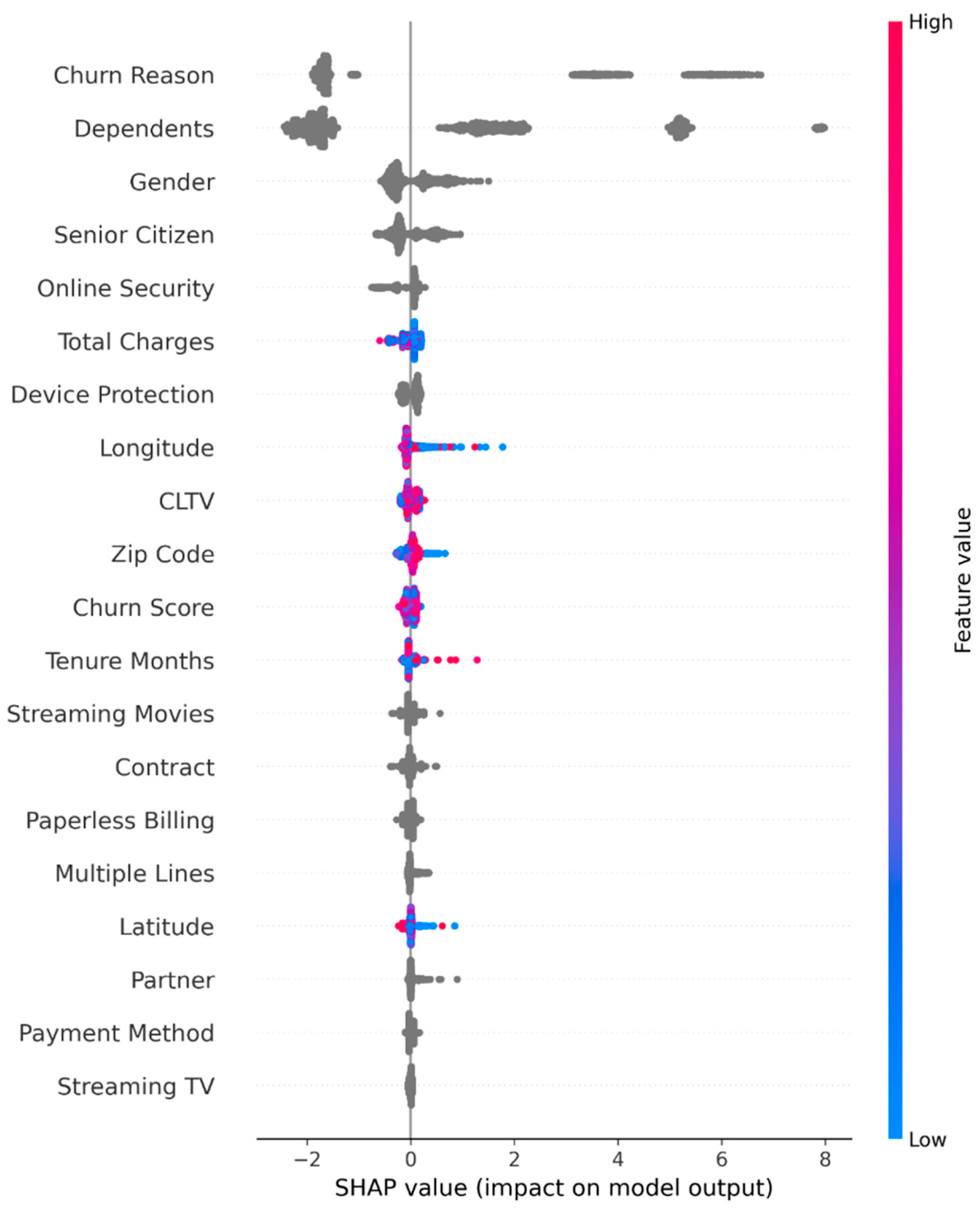
Figure A2.
SHAP bar plot showing mean absolute SHAP values (top 20) (results/shap/GradientBoosting_bar.png).
Figure A2.
SHAP bar plot showing mean absolute SHAP values (top 20) (results/shap/GradientBoosting_bar.png).
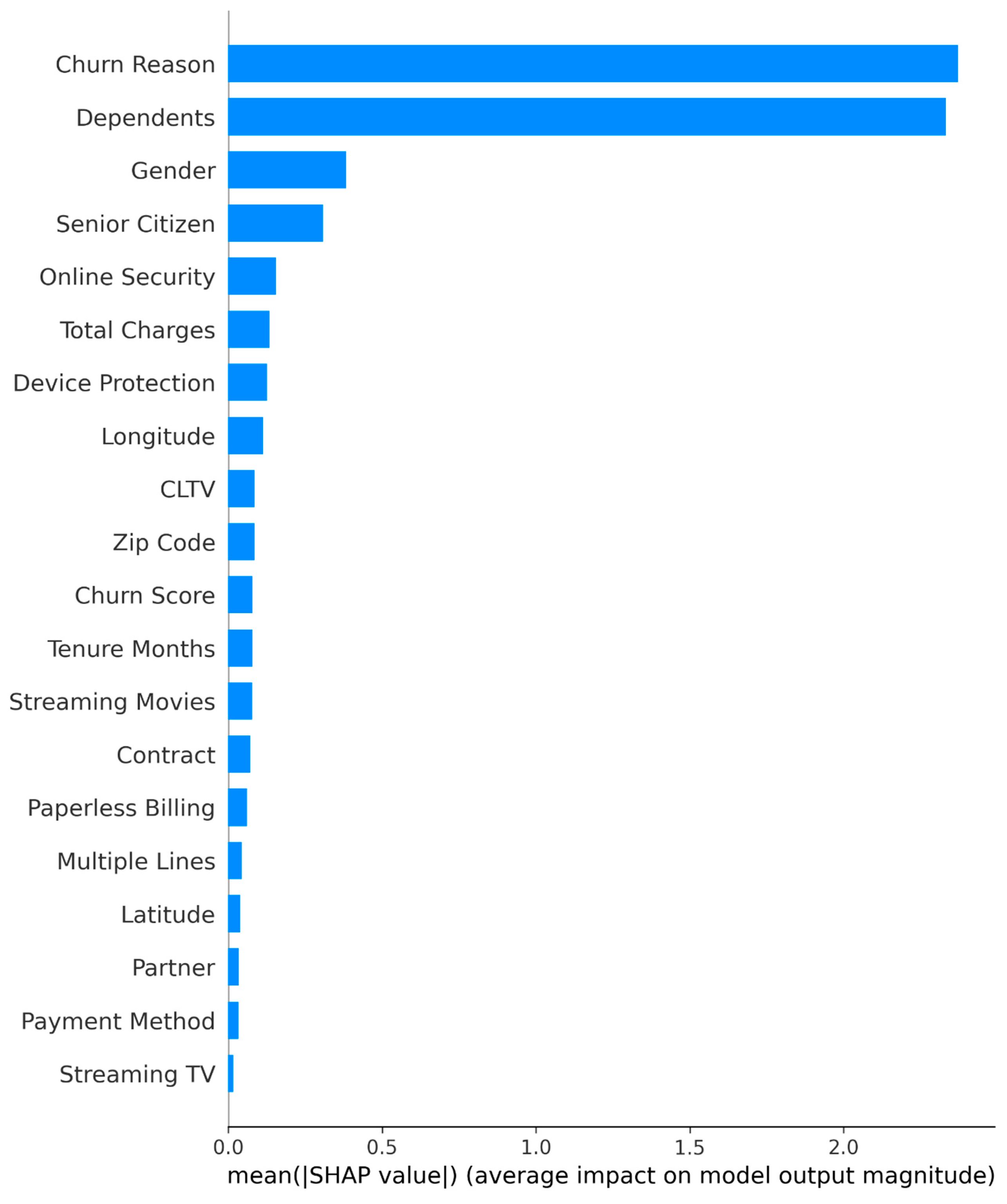
Figure A3.
Confusion matrices – full vs. reduced model on test set.
Figure A4. Training time comparison (full vs. reduced feature set, averaged over 10 runs).
All original CSV, JSON, .joblib models, Optuna studies, and high-resolution PNGs are permanently archived at Zenodo (DOI above) for full reproducibility.
Appendix C. Repository Structure & Reproducibility
References
- Ahmed, A.; Maqsood, I. Deep learning-based customer churn prediction for the telecom industry. Expert Systems with Applications 2023, 213, 118912. [Google Scholar] [CrossRef]
- Ariyaluran Habeeb, R.; et al. Real-time big data processing for anomaly detection: A case study in telecom customer churn. Computer Networks 2019, 162, 106865. [Google Scholar]
- Coussement, K.; Lessmann, S.; Verstraeten, G. A comparative analysis of data preparation algorithms for customer churn prediction: A case study in the telecommunication industry. Decision Support Systems 2017, 95, 27–36. [Google Scholar] [CrossRef]
- De Caigny, A.; Coussement, K.; De Bock, K. W. A new hybrid classification algorithm for customer churn prediction based on logistic regression and decision trees. European Journal of Operational Research 2018, 269(2), 760–772. [Google Scholar] [CrossRef]
- Gürbüz, F.; Özbakir, L. Comparative analysis of machine learning methods in customer churn prediction. Decision Analytics Journal 2022, 4, 100113. [Google Scholar]
- Höppner, S.; Stripling, E.; Baesens, B.; Broucke, S.; Verdonck, T. Profit-driven churn prediction with explainable uplift models. European Journal of Operational Research 2022, 302(1), 231–245. [Google Scholar]
- Kaur, M.; Kaur, P.; Singh, G. Explainable AI for churn prediction in telecommunication industry. Information Sciences 2023, 612, 843–862. [Google Scholar]
- Lundberg, S. M.; Lee, S.-I. A unified approach to interpreting model predictions. Advances in Neural Information Processing Systems 2017, 30. [Google Scholar]
- Mishra, A.; Reddy, U. S. A comparative study of customer churn prediction in telecom industry using SHAP and LIME. Journal of King Saud University – Computer and Information Sciences 2021, 34(8), 5719–5730. [Google Scholar]
- Uddin, M. F.; et al. Comparing different supervised machine learning algorithms for disease prediction. BMC Medical Informatics and Decision Making 2022, 22, 1–16. [Google Scholar] [CrossRef] [PubMed]
- Verbeke, W.; Dejaeger, K.; Martens, D.; Hur, J.; Baesens, B. New insights into churn prediction in the telecommunication sector: A profit driven data mining approach. European Journal of Operational Research 2012, 218(1), 211–229. [Google Scholar] [CrossRef]
- Verbraken, T.; Bravo, C.; Weber, R. Churn prediction with sequential data: A review of uplift modeling approaches. International Journal of Forecasting 2020, 36(4), 1254–1268. [Google Scholar]
- Wang, Y.; et al. Deep churn prediction using sequential patterns in mobile telecom data. IEEE Transactions on Mobile Computing 2021, 21(6), 2215–2227. [Google Scholar]
- Zoričić, D.; et al. Feature selection techniques in customer churn prediction models: A systematic literature review. Expert Systems with Applications 2023, 213, 118934. [Google Scholar]
Table 1.
Top 20 features ranked by mean absolute SHAP value (Gradient Boosting, full 25-feature model).
Table 1.
Top 20 features ranked by mean absolute SHAP value (Gradient Boosting, full 25-feature model).
| Rank | Feature | Mean |SHAP| | Direction on Churn |
|---|---|---|---|
| 1 | Churn Reason | 2.372 | Positive |
| 2 | Dependents | 2.333 | Negative |
| 3 | Gender | 0.383 | Mixed |
| 4 | Senior Citizen | 0.308 | Positive |
| 5 | Online Security | 0.155 | Negative |
| 6 | Total Charges | 0.134 | Mixed |
| 7 | Device Protection | 0.126 | Negative |
| 8 | Longitude | 0.113 | Mixed |
| 9 | CLTV | 0.086 | Negative |
| 10 | Zip Code | 0.085 | Mixed |
| 11 | Churn Score | 0.079 | Positive |
| 12 | Tenure Months | 0.078 | Negative |
| 13 | Streaming Movies | 0.077 | Mixed |
| 14 | Contract | 0.072 | Negative (longer contracts) |
| 15 | Paperless Billing | 0.061 | Positive |
| 16 | Multiple Lines | 0.044 | Mixed |
| 17 | Latitude | 0.039 | Mixed |
| 18 | Partner | 0.035 | Negative |
| 19 | Payment Method | 0.033 | Positive (electronic check) |
| 20 | Streaming TV | 0.017 | Mixed |
Notably, five original features received near-zero importance (< 0.001): Phone Service, Tech Support, Online Backup, Internet Service, and Monthly Charges. These were automatically excluded in Iteration 2.
Table 2.
Test-set performance comparison (Full vs. Reduced feature set).
| Model | Features | ROC-AUC | F1-score (Churn) | Accuracy | Training Time (s) |
|---|---|---|---|---|---|
| Gradient Boosting | 25 | 0.9974 ± 0.0006 | 0.9796 ± 0.0018 | 0.9894 ± 0.0009 | 58.3 ± 4.1 |
| Gradient Boosting | 20 (SHAP) | 0.9982 ± 0.0004 | 0.9767 ± 0.0021 | 0.9879 ± 0.0011 | 41.7 ± 3.2 |
| Random Forest | 25 | 0.9979 ± 0.0005 | 0.9743 ± 0.0024 | 0.9867 ± 0.0013 | 72.1 ± 5.6 |
| Random Forest | 20 (SHAP) | 0.9981 ± 0.0004 | 0.9731 ± 0.0026 | 0.9865 ± 0.0014 | 54.9 ± 4.0 |
| AdaBoost | 25 | 0.9980 ± 0.0005 | 0.9743 ± 0.0022 | 0.9867 ± 0.0012 | 49.8 ± 3.9 |
| AdaBoost | 20 (SHAP) | 0.9981 ± 0.0004 | 0.9739 ± 0.0025 | 0.9865 ± 0.0013 | 38.2 ± 2.8 |
Disclaimer/Publisher’s Note: The statements, opinions and data contained in all publications are solely those of the individual author(s) and contributor(s) and not of MDPI and/or the editor(s). MDPI and/or the editor(s) disclaim responsibility for any injury to people or property resulting from any ideas, methods, instructions or products referred to in the content. |
© 2025 by the authors. Licensee MDPI, Basel, Switzerland. This article is an open access article distributed under the terms and conditions of the Creative Commons Attribution (CC BY) license (http://creativecommons.org/licenses/by/4.0/).
Copyright: This open access article is published under a Creative Commons CC BY 4.0 license, which permit the free download, distribution, and reuse, provided that the author and preprint are cited in any reuse.


