
Submitted:
07 July 2025
Posted:
09 July 2025
You are already at the latest version
Abstract
In the subscription-based publishing industry, customer churn poses a significant challenge to business sustainability, as acquiring new customers is substantially more costly than retaining existing ones. This study examines the development of an automated churn prediction pipeline for S.P. AbonneeService, a B2B subscription service provider managing over 200 titles and 350,000 end-consumers across multiple publishing categories. The research implements a comprehensive machine learning framework utilizing the CRISP-DM methodology, evaluating six algorithms (Naive Bayes, Logistic Regression, Random Forest, XGBoost, LightGBM, SVM) across three resampling techniques and three temporal validation strategies using five years of historical subscription data from three distinct publishing companies. The automated preprocessing pipeline addresses heterogeneous data structures, seasonal variance, and class imbalance through systematic feature engineering, temporal validation, and synthetic minority oversampling. Experimental results demonstrate that LightGBM with SMOTE resampling achieves superior performance across all evaluated contexts, with AUC-PR values exceeding 0.95 and precision rates above 0.95 for top-performing configurations. The study establishes that automated churn prediction systems can deliver exceptional predictive performance while maintaining interpretability essential for actionable retention strategies, enabling subscription publishing companies to implement advanced predictive capabilities that directly support customer retention.
Keywords:
churn prediction
; machine learning
; subscription publishing
; automated pipeline
; class imbalance
; SMOTE
; temporal validation
; gradient boosting
; customer retention
1. Introduction
1.1. Background and Significance
In the subscription-based publishing industry, customer churn, defined as the percentage of customers who discontinue their subscriptions within a given time period [1], poses a significant challenge to business sustainability. The subscription business model has gained prominence across various sectors in recent years, with the publishing industry experiencing a notable shift from traditional one-time purchases to recurring revenue structures [2]. This shift has made subscriber retention a critical factor for revenue stability and growth potential, as research continues to demonstrate that acquiring new customers is substantially more costly than retaining existing ones [3].
Churn prediction is a critical analytical approach within subscription-based industries, enabling organizations to proactively identify customers at risk of discontinuing their service. By leveraging machine learning and advanced data analytics, companies can analyze historical customer behavior, transactional patterns, demographics, and interactions to detect early indicators of churn [4]. This predictive capability is especially valuable in subscription models, where recurring revenue and long-term customer relationships are central to business sustainability.
This study examines S.P. AbonneeService, a well-established subscription-based service company within the publishing sector, as its case company. With over 20 years of industry experience, S.P. AbonneeService has developed an extensive portfolio encompassing more than 200 titles (individual publications such as magazines, journals, and newspapers) and 350,000 end-consumers across various publishing categories, making it a significant industry participant. This substantial customer portfolio presents both an opportunity and a challenge for retention strategies, as even minor improvements in churn reduction can translate to considerable revenue preservation given the scale of their operations.
Traditional churn prediction typically focuses on single datasets where manual tuning and adjustment are feasible; however, in B2B contexts like S.P. AbonneeService, this approach is no longer viable. Extensive manual recalibration for each client takes a significant amount of time, which is why an automated churn prediction pipeline is vital for B2B companies such as S.P. AbonneeService. Automated pipelines effectively address the computational challenges presented by multi-client environments through adaptive preprocessing and model selection mechanisms that maintain prediction accuracy across different data distributions, eliminating the need for extensive human intervention with each implementation. Research demonstrates that such automated frameworks can reduce the resource-intensive nature of feature engineering, which typically dominates the development effort in production inference pipelines, while maintaining or even improving predictive performance across diverse client datasets [6,7]. From a strategic perspective, these capabilities would enable S.P. AbonneeService to deliver consistent, scalable churn prediction services across their entire client portfolio, enhancing their value proposition while contributing to the broader academic understanding of generalizable retention methodologies in subscription-based industries.
1.2. Current State of Research
Churn prediction methodologies typically utilize two primary approaches: survival analysis and binary classification, each offering distinct advantages for subscription-based industries. Survival analysis, initially developed for clinical trials and medical research, offers sophisticated temporal modeling capabilities that are particularly valuable when dealing with censored data. Censored data refers to situations where the event of interest (churn) has not occurred by the end of the observation period [14]. This approach commonly utilizes techniques such as the Kaplan-Meier estimator to predict the probability distribution of time until churn, enabling organizations to not only understand whether customers will churn but also when such events are more likely to occur. Research demonstrates that survival analysis can reveal substantial customer lifetime values, with studies showing average survival times extending beyond 200 days in specific subscription contexts, providing business-critical insights for revenue forecasting and timing retention strategies [14].
Binary classification approaches, conversely, focus on categorical prediction by assigning customers to one of two states: likely to churn or likely to remain active within a specified prediction window. This methodology emphasizes learning functions that minimize misclassification probability through various machine learning algorithms, including logistic regression, support vector machines, and ensemble methods such as random forests [14]. Binary classification proves particularly valuable for operational decision-making, as it enables clear “intervene or don't intervene” determinations that translate directly into actionable retention strategies. Recent empirical studies demonstrate that advanced binary classification models can achieve ROC AUC scores exceeding 0.96 for six-month churn prediction horizons, indicating robust predictive performance across diverse subscription environments [14]. The choice between survival analysis and binary classification often depends on organizational requirements, with survival analysis providing richer insights into temporal dynamics. In contrast, binary classification offers a more straightforward implementation for automated intervention systems.
Traditional statistical approaches have been largely superseded by machine learning techniques that demonstrate superior predictive capabilities. A comprehensive survey spanning an entire decade of research reveals that machine learning applications in telecom churn prediction have become progressively more refined, moving beyond basic classification to incorporate more nuanced behavioral analysis [9]. These advances have extended beyond telecommunications to various subscription-based industries, including banking, publishing, and digital services [12].
1.2.1. Evolution of Machine Learning Techniques
The evolution of machine learning applications in churn prediction has undergone a significant transition from traditional logistic regression models to sophisticated ensemble methods, which demonstrate superior predictive capabilities. Early approaches primarily relied on logistic regression and Naive Bayes classifiers, which provided interpretable results but often struggled with complex non-linear relationships in customer behavior data [5,28]. Logistic regression models typically achieved accuracy rates around 80-90%, demonstrating reasonable performance but with limitations in handling non-linear separability in complex datasets [9,12,28]. Support Vector Machines (SVM) emerged as an improvement, particularly when enhanced with optimization techniques such as Grey Wolf Optimization, consistently outperforming standard models like logistic regression, Naive Bayes, and decision trees in telecommunications churn prediction [5,9].
The introduction of ensemble methods has marked a significant shift in churn prediction accuracy and robustness. Random Forest algorithms have gained widespread adoption due to their stability, interpretability, and effectiveness in handling moderately imbalanced datasets, with studies reporting accuracy rates ranging from 89% to 95% and demonstrating a strong capability in managing large telecommunications datasets [5,9,28]. Gradient boosting algorithms, particularly XGBoost and LightGBM, have shown exceptional performance across multiple studies, with XGBoost achieving accuracy rates of 99.99% and perfect ROC AUC scores of 1.0 in recent evaluations [28]. LightGBM has demonstrated superior performance compared to traditional methods, such as SVM, Random Forest, and even XGBoost, in financial dataset contexts, particularly when enhanced with focal loss functions to address class imbalance challenges. This approach achieves a churn detection rate of 0.94 with an AUC score of 0.99 [5]. These ensemble methods excel at capturing complex patterns and interactions in customer data while maintaining reasonable computational efficiency, making them particularly suitable for production environments where both accuracy and scalability are critical [27,28].
1.2.2. Data Handling and Validation
The effectiveness of churn prediction models depends significantly on feature selection and data preparation processes. Recent studies have highlighted that these preliminary stages often determine model performance more than the choice of algorithm itself [10]. Research from 2022 emphasizes that while manual feature selection remains common in the telecom industry, automated selection methods are gaining prominence, with Fisher Score (a filter method) and Random Forest (an embedded method) emerging as the most effective approaches [10].
Temporal validation frameworks are a crucial consideration in churn prediction development, as traditional random sampling approaches can lead to data leakage and overly optimistic performance estimates. Research has demonstrated the importance of chronological data splitting, where models are trained on historical data and tested on future periods to emulate real-world deployment scenarios [28]. The most comprehensive temporal validation approach identified in current literature involves rolling-window cross-validation, which enables continuous training on expanding historical data while testing on subsequent time periods, thereby ensuring models learn from past customer behavior patterns and can adapt to future trends [28]. This methodology helps identify concept drift and triggers adaptive retraining when model performance degrades beyond predefined thresholds, typically measured by drops in ROC AUC or F1-score exceeding 5% [28].
Cross-validation techniques have been extensively utilized in churn prediction research, with k-fold cross-validation (typically k = 5 or k = 10) being the most common approach for model validation and hyperparameter tuning [11,12,14,28]. Stratified sampling methods have been recognized as essential for maintaining the original churn ratio in training and test sets, preventing models from being biased toward the majority class [12,28]. However, despite these advances, current research reveals that specialized temporal validation strategies explicitly designed for subscription-based business contexts remain limited, with most studies adapting general machine learning validation techniques rather than developing domain-specific approaches.
Class imbalance handling techniques have become increasingly sophisticated, addressing the fundamental challenge that churned customers typically represent a minority class in most subscription datasets. The Synthetic Minority Over-sampling Technique (SMOTE) has emerged as the most widely adopted approach, generating synthetic samples to balance class distributions and enhance model performance, particularly when combined with ensemble methods such as XGBoost and Random Forest [2,5,12,27,28]. Research demonstrates that SMOTE implementation with ensemble learning enhances classification performance by addressing class imbalance and improves F1-Score through various classification algorithms and voting strategies [5,27]. Advanced variants such as Adaptive Synthetic Sampling (ADASYN) have been developed to focus on generating synthetic instances around minority class instances that are more challenging to learn, employing weighting systems based on learning difficulty [5,27]. Hybrid approaches combining SMOTE with Edited Nearest Neighbors (ENN) have demonstrated superior performance, with hybrid SMOTE-ENN approaches achieving F1 scores exceeding 95% in telecommunications datasets [5].
Recent research has explored additional sampling techniques, including Gaussian Noise Upsampling (GNUS) and various undersampling methods such as Random Undersampling, NearMiss, and Tomek Links [5,27]. The selection of appropriate sampling techniques has been shown to depend significantly on the specific degree of class imbalance and the chosen classification algorithm. Studies indicate that XGBoost consistently outperforms Random Forest across all sampling methods, particularly showing substantial improvements when combined with GNUS in extremely imbalanced scenarios [27].
1.2.3. Evaluation Metrics
Appropriate evaluation metrics for imbalanced classification scenarios have become increasingly important as traditional accuracy measures can be misleading when dealing with skewed class distributions. Recent research emphasizes the importance of comprehensive evaluation sets of metrics, including precision, recall, F1-score, and the Matthews Correlation Coefficient (MCC), to provide balanced assessments of model performance [3,5,9,27,28]. Precision measures how many predicted churn customers were actual churners, minimizing false positives, while recall assesses how well models capture actual churned customers, aiming to reduce false negatives [12,28]. The F1-score, as the harmonic mean of precision and recall, provides a balanced evaluation, particularly suitable for imbalanced datasets where both types of errors have essential business implications [3,27,28].
The Matthews Correlation Coefficient (MCC) has gained particular prominence as it considers all four quadrants of the confusion matrix, providing a more comprehensive measure that ranges from -1 to 1, where values closer to 1 indicate superior predictive performance even in highly imbalanced datasets [27,28]. The Area Under the Precision-Recall Curve (AUC-PR) has emerged as particularly valuable for churn prediction, as it focuses on the minority class performance and provides more informative insights than traditional ROC curves when positive class prediction is critical [27]. ROC AUC remains essential for assessing discriminatory power across various thresholds, with scores closer to 1.0 indicating superior model effectiveness in distinguishing between churn and non-churn cases [3,12,28]. Log loss has become essential for evaluating probabilistic predictions, with lower values indicating more accurate and well-calibrated probability estimates, which are crucial for ranking customers by their churn risk [28].
1.2.4. Automated Pipeline
The emergence of automated machine learning (AutoML) represents one of the most significant recent developments in churn prediction research. Traditional model development requires extensive manual tuning, which becomes impractical in multi-client B2B environments, such as S.P. AbonneeService. To address this limitation, researchers have developed automated pipeline frameworks that streamline the model development process [7].
1.2.5. Research Gaps and Domain-Specific Challenges
Despite these advances, significant gaps remain in current churn prediction research, particularly regarding the cross-publisher applicability and handling of seasonal variance. The scholarly publishing industry has received limited attention, with the first empirical study on customer churn prediction in this sector not appearing until 2022 [11]. This study highlighted the unique characteristics of academic publishing subscriptions and proposed methods for predicting customer defection based on 6.5 years of subscription data from a major educational publisher [11].
Recent research has begun addressing the challenge of seasonality in subscription-based businesses. A February 2025 study proposes a simplified and numerically stable approach to the BG/NBD churn prediction model, specifically designed for industries where customer behavior is influenced by seasonal events [8]. This model modifies the traditional definition of churn to account for purchase patterns over extended periods, making it potentially valuable for publishing businesses with seasonal subscription behaviors.
Building on the research gaps identified above, our analysis reveals several interconnected challenges that must be addressed when developing effective churn prediction models for S.P. AbonneeService:
- Seasonality: Subscription-based publishing exhibits significant seasonal fluctuations in customer behavior that complicate churn prediction efforts. As noted in recent research, customer behavior is often heavily influenced by seasonal events, creating irregular patterns that standard prediction models struggle to capture accurately [8]. For S.P. AbonneeService, this is displayed as fluctuating engagement metrics across different times of the year, with subscription renewal decisions frequently clustering around specific calendar periods rather than being evenly distributed. These temporal patterns create complex challenges for machine learning models that must distinguish between temporary seasonal disengagement and genuine pre-churn behavior.
- Dataset heterogeneity: S.P. AbonneeService operates as a B2B service provider across more than 200 titles and 350,000 end-consumers spanning multiple publishing categories. This inherently creates significant data heterogeneity challenges, as each publisher partner maintains a unique customer base with distinct behavioral patterns, engagement metrics, and churn triggers. Subscription terms, pricing models, and content delivery mechanisms vary substantially among publishers, resulting in inconsistent data structures and relationship patterns. Additionally, the varying lengths of partnership histories result in uneven data maturity levels, with some publishers providing rich historical datasets while others offer limited behavioral timelines. Further complicating matters, publishers with extensive histories often include conversion data from customers who transferred from previous service providers. This data is frequently poorly structured, inconsistently formatted, and missing key relationship details critical for accurate churn prediction.
- Class imbalance: Across all publishers in our dataset, an average of 54.51% of customers (excluding trial memberships and non-actionable cancellations) are classified as inactive. For publishers with longer partnership histories, this imbalance becomes particularly challenging for predictive modeling as the distribution of active versus inactive customers can vary significantly. This challenge aligns with broader research findings, where imbalanced datasets often lead to biased model performance, reducing overall effectiveness [5]. When data is skewed toward one class, traditional models tend to favor the dominant class, producing good accuracy metrics but poor performance in identifying the minority class [5].
- Interpretability requirements: In today's business environment, stakeholders increasingly demand transparency and understanding of predictive analytics outcomes [3]. As Maan and Maan [3] emphasize, “explainability and transparency are of major concerns identified by Customers across business domains”. For S.P. AbonneeService, interpretable predictions are essential for translating predictions into actionable retention strategies. Management requires clear insights into why specific customers are flagged as churn risks, enabling the design of targeted interventions that address the root causes rather than just the symptoms. This transparency requirement aligns with growing industry recognition that “there is a dire need to design, develop and deploy machine learning models which are ethical in their purpose, design and usage, covering key aspects of transparency, explainability and interpretability” [3].
- Temporal validation limitations: Although existing research has established the importance of temporal validation through rolling-window cross-validation approaches [28], comprehensive frameworks designed explicitly for subscription-based business contexts remain limited. Current validation methodologies primarily adapt general machine learning techniques, rather than addressing the unique temporal patterns and seasonal behaviors characteristic of subscription publishing environments. This creates a need for more specialized validation strategies that can effectively handle the complex temporal dynamics inherent in multi-client publishing contexts.
1.3. Research Question
This study addresses the critical challenge of developing scalable, automated churn prediction capabilities for multi-client subscription publishing environments. Given the complex operational realities identified in the current research landscape, this investigation focuses on creating practical solutions that can function effectively across diverse publisher portfolios. The primary research question guiding this study is: How can an AI model be developed to predict customer churn, enabling the effective implementation of proactive retention measures?
The question emphasizes the explicit proactive application of predictions, recognizing that prediction accuracy alone is insufficient without corresponding actionable insights for implementing retention strategies.
To systematically address this primary question, this study adopts the Cross-Industry Standard Process for Data Mining (CRISP-DM) methodology, which has served as the de facto standard for data mining projects across industries since its introduction in 2000. CRISP-DM provides a structured framework consisting of six iterative phases: Business Understanding, Data Understanding, Data Preparation, Modeling, Evaluation, and Deployment [13]. This methodology is particularly well-suited for the multi-client B2B environment of S.P. AbonneeService, as it emphasizes thorough business and data understanding, and provides a systematic approach that is essential for automated churn prediction systems operating on a heterogeneous dataset. By following CRISP-DM's structured approach, this research ensures that both theoretical rigor and practical implementation requirements are addressed throughout the model development lifecycle.
1.4. Delimitations and Scope
This research establishes specific boundaries to ensure focused investigation and clear evaluation criteria for the automated churn prediction system. The study focuses exclusively on binary classification approaches to churn prediction, where customers are classified as either likely to churn or likely to remain active within the specified prediction window. This methodological choice aligns directly with S.P. AbonneeService's operational requirements, as binary predictions enable clear “intervene or don't intervene” decisions that translate immediately into actionable retention strategies. Alternative methodological approaches, including survival analysis techniques, fall outside the scope of this investigation. The research emphasizes machine learning techniques specifically chosen for their balance between predictive performance and interpretability requirements, prioritizing models that can provide clear, actionable insights to business stakeholders rather than pursuing potentially marginal performance improvements through less interpretable deep learning approaches.
Given that S.P. AbonneeService's client portfolio consists entirely of subscription-based publishers within traditional publishing categories, such as magazines, newspapers, and general literature, the research scope naturally aligns with these publishing sectors. The research exclusively addresses multi-client B2B environments, where service providers like S.P. AbonneeService manage subscription services for multiple independent publishers, as opposed to direct-to-consumer or single-publisher environments.
This study focuses on generating predictions for a one-month prediction horizon, aligning with the most prevalent subscription billing cycles within S.P. AbonneeService's client portfolio while providing sufficient lead time for implementing targeted retention measures. The analysis is restricted to actionable end-consumers, specifically excluding trial membership customers and those whose subscription cancellations result from unactionable circumstances such as payment failures or administrative issues. This customer segmentation approach ensures that the predictive model focuses on behavioral churn patterns that can be addressed through targeted retention interventions, maximizing the practical value of predictions for retention strategy implementation.
2. Materials and Methods
Figure 1 provides a comprehensive overview of the automated churn prediction pipeline developed for multi-client subscription publishing environments. The workflow illustrates the systematic progression from raw database exports through the seven-stage preprocessing pipeline, followed by the experimental evaluation framework that systematically combines temporal validation strategies, machine learning algorithms, and resampling techniques to generate 54 distinct experimental configurations. This integrated pipeline addresses the fundamental challenges of data heterogeneity, temporal dependencies, and class imbalance inherent in subscription publishing contexts, with each component described in detail in the subsequent sections.
2.1. Data Description
The foundation of this study rests upon the export data from S.P. AbonneeService's database systems. This dataset represents a complete cross-sectional snapshot of subscription-related information, encompassing behavioral, transactional, and demographic patterns essential for churn prediction modeling.
The dataset architecture is organized into four sections that collectively capture the subscription lifecycle and dynamics of the customer relationship. These categories include Subscriber Data, Subscription Data, Invoice Data, and Statistical Data, each serving distinct analytical purposes. This approach enables a comprehensive analysis of customer behavior patterns while preserving the details necessary for accurate churn prediction across heterogeneous publisher environments.
2.1.1. Subscriber Data
The subscriber data component encompasses comprehensive demographic, contact, and preference information for both subscription recipients and financial payers within the subscription ecosystem. This dual-entity structure acknowledges the complexity of modern subscription relationships, particularly in gift subscription scenarios where the beneficiary and financial responsible party represent distinct individuals with separate behavioral profiles and communication preferences.
Recipient subscriber data captures complete customer profiles including personal identification details, comprehensive address information spanning street-level specificity through international postal systems, and multi-channel contact information encompassing various email addresses, telephone numbers, and traditional correspondence methods. The demographic component includes gender classification, formal titles, and complete name structures that accommodate international naming conventions and cultural variations across S.P. AbonneeService's diverse customer base.
Financial and administrative elements within subscriber data include banking information necessary for payment processing, tax identification numbers for compliance purposes, and detailed communication preferences that govern customer contact permissions.
Payer subscriber data maintains an identical structure to recipient data, populated exclusively in scenarios where the subscription financial responsibility differs from that of the subscription beneficiary. This approach enables complete analysis for gift subscription scenarios while maintaining data integrity through consistent field structures and validation requirements across both subscriber entity types.
2.1.2. Subscription Data
Subscription data represents the core analytical component of the dataset, containing detailed information about individual subscription instances and their lifecycle characteristics. Each subscription record maintains a unique identification spanning over 200 titles across multiple publishing categories within S.P. AbonneeService's scope.
Publication-specific information, including content type, delivery method, and editorial focus, enables analysis across different forms of publishing. Subscription acquisition data captures the complete customer journey, from the initial contact method to detailed source attribution, promotional campaign identification, and registration methodology, enabling effective marketing analysis and informed decision-making.
Pricing and payment structures within subscription data include detailed tariff classifications, payment frequency specifications, and delivery quantity tracking, which accommodates varying subscription models ranging from weekly publications to quarterly journals. The payment processing component tracks both completed transactions and obligations.
Subscription lifecycle management data captures the temporal evolution of customer relationships through comprehensive tracking of start and end dates, renewal behavior patterns, and administrative status modifications. Cancellation data provides detailed attribution, including methodology employed, underlying reasons for discontinuation, and timing patterns that reveal seasonal and behavioral trends essential for predictive modeling.
2.1.3. Invoice Data
The invoice data component provides a focused snapshot of the most recent billing interaction for each subscription, representing the current financial status rather than comprehensive historical billing records.
Current invoice information includes detailed billing identification, transaction timing, and comprehensive payment status classification that distinguishes between various stages of the billing lifecycle. Payment status tracking encompasses initial invoicing confirmation, successful payment completion, automated banking debits, and identification of outstanding balances, providing essential indicators of customer financial engagement and potential payment-related churn triggers.
Collection and reminder data within the invoice component tracks customer response patterns to payment requests, including detailed timing of reminder communications and customer payment behavior following collection efforts. This information provides critical insights into financial issues and payment pattern disruptions that frequently precede subscription cancellation decisions, making it particularly valuable for predictive modeling focused on payment-related churn scenarios.
2.1.4. Statistical Data
The statistical data component serves a dual purpose, containing both processed derivatives of the primary data categories and unique metrics that cannot be derived from the base data alone. The processed elements provide standardized versions of subscriber, subscription, and invoice information.
The primary value of statistical data lies in its behavioral and interaction metrics, which extend beyond transactional records to capture service quality indicators and patterns of customer relationships. Delivery performance tracking encompasses detailed complaint histories and service interruption patterns, reflecting operational effectiveness and customer satisfaction levels. These metrics provide essential context for understanding non-financial churn triggers related to service quality and operational performance. Customer service interaction data within the statistical component reveals customer engagement patterns by facilitating the number of interactions with customer service.
Historical subscription patterns captured within statistical data offer complex insights into customer behavior that extend beyond current subscription status. These metrics include subscription duration tracking, renewal pattern analysis, and cross-portfolio subscription behavior, which reveals customer lifecycle patterns essential for developing a comprehensive retention strategy.
2.2. Data Preprocessing
The raw data extracted from S.P. AbonneeService’s systems undergoes an extensive automated preprocessing pipeline to ensure data quality, consistency, and suitability for the full churn prediction pipeline. This pipeline is designed to be robust across diverse publisher datasets and prioritizes the creation of interpretable features. The sequence of operations is carefully structured: initial standardization and cleaning prepare the data for reliable feature engineering, which is then followed by refinement, missing value imputation, and advanced numerical processing to optimize the dataset for machine learning algorithms.
2.2.1. Initial Data Cleaning and Standardization
The first stage focuses on foundational data integrity. All raw data fields are subjected to type conversion: date-like strings are parsed into standardized datetime objects; numeric fields, including those representing currency with associated symbols and locale-specific decimal separators, are converted to numerical types; boolean-like text (e.g., “Ja”/“Nee”, which is Dutch for “Yes”/“No”) is mapped to true boolean values; and fields intended as categorical are defined as categorical variables, with common string representations of missingness (e.g., “nan”, “none”, empty strings) unified to a standard null representation. For instance, gender indicators are transformed to a consistent case. Any remaining columns not explicitly typed are converted to a string format. A minimal rule-based normalization, driven by configurable patterns, is then applied to specific fields to rectify common inconsistencies, although current configurations apply this sparingly. This initial standardization is crucial as it ensures that all subsequent operations act upon data of expected and consistent types, preventing errors and improving the reliability of derived features.
2.2.2. Feature Engineering and Enrichment
Following initial cleaning, several feature engineering steps are undertaken to create new, more informative variables.
First, a set of binary indicators is generated from existing data characteristics. For example, the presence of contact information, such as an email address or phone number, or the use of specific payment methods, such as direct debit, is converted into boolean flags. This binarization enhances model interpretability by creating explicit signals for key customer attributes, thereby improving the model's clarity and transparency.
Second, more complex derived features are created to capture crucial aspects of subscriber behavior and lifecycle. Subscriber birth dates are transformed into age categories; this categorization can be static or adaptive to the data distribution, based on pipeline configuration, to ensure meaningful group sizes. Additionally, behavioral patterns such as serial churn tendencies are identified by analyzing historical subscription patterns. The specific criteria for flagging a customer as a serial churner, namely an average subscription duration of less than one year, more than two cancelled subscriptions, and more than three total subscriptions, were established based on industry experience and the recommendation of S.P. AbonneeService's CTO, Marc Dierikx [15]. A significant step involves calculating churn indicators: a binary churn event flag is determined based on subscription end dates and renewal statuses, and a corresponding time-to-event (or time-to-censoring for active subscriptions) is computed relative to a defined study end date, which can be utilized for future survival analysis. This provides the target variable and temporal context for the churn model. Summaries of customer interactions, including the total number of service issues or issues per year (calculated using Bayesian smoothing and percentile capping to handle variance and outliers), are also generated.
Third, composite scores are engineered by combining several binarized features with predefined weights. These scores aim to quantify abstract concepts, including customer reachability (based on available contact channels and permissions), engagement (based on communication opt-ins), business customer profile strength (based on the provision of business-specific details, such as VAT numbers), and payment reliability (based on payment method and reminder history). The specific features included in these composite scores and their respective weights were determined in consultation with Marc Dierikx [15] to reflect business understanding and their relative importance. These engineered features provide higher-level abstractions that can be more directly interpretable and predictive.
2.2.3. Data Filtering and Refinement
To focus the analysis on relevant customer segments, specific data filtering rules are applied. Rows corresponding to non-actionable subscription types or particular business-to-business intermediary accounts, as defined in the configuration based on criteria provided by Marc Dierikx [15], are removed. Additionally, scenarios where the financial payer is a distinct entity from the subscription recipient are filtered out to simplify the modeling scope, focusing on direct subscriber relationships. This step ensures the model is trained on a dataset representative of the target population for retention efforts.
2.2.4. Missing Value Imputation
The pipeline then addresses missing data through a multi-faceted imputation strategy. The placement of this comprehensive imputation stage within the pipeline is a considered choice. Initial data cleaning and type conversion (Section 2.2.1) standardize various raw representations of missingness to null values. Early feature engineering steps, particularly binarization (Section 2.2.2), often rely on the distinction between present and absent data, thus implicitly using the original missingness context (e.g., a customer either has a listed phone number or not). However, the creation of other derived features, such as calculating age from birth dates, can introduce new missing values if the source data is incomplete. Therefore, the main imputation phase is strategically positioned after these initial feature creation steps but critically before the advanced numerical processing stages (Section 2.2.6), such as skewness correction and outlier treatment, and subsequent model training. These later stages generally require complete, non-null datasets to function correctly and produce reliable results. This ordering ensures that as much information as possible is derived while preserving the original missingness context where beneficial, before filling gaps to prepare for numerically intensive algorithms.
For geographical information, missing province data for subscribers is imputed using a hierarchical approach. First, suppose the subscriber's country code indicates a non-domestic location, a distinct "Foreign_[CountryCode]" category is assigned. In this case, the reason is that province-level data is not consistently recorded for international subscribers, and the relatively low volume of such subscribers makes detailed imputation impractical and less reliable. For domestic (Dutch) addresses with missing provinces, the system attempts to infer the province by first looking up the most common province associated with the subscriber's listed city or place name from non-missing records. If this fails, it then attempts to infer the province based on the most common province associated with the initial digits of their postal code. Any remaining domestic addresses with unidentifiable provinces are assigned an "Unknown_NL" category, while truly unclassifiable cases default to a general "Unknown" province.
Beyond these targeted imputations, a general configurable strategy handles remaining missing values. Depending on the configuration (e.g., AUTOFILL_MISSING), missing numerical data may be filled with zero, booleans with false, and categoricals with a distinct “Unknown” category. Specific columns, such as counts of items sent or paid, may have custom default fill values (e.g., 1). The critical subscription cancellation date is explicitly preserved as missing if KEEP_OPZEGDATUM is enabled, which will mainly be used for auditing purposes in later steps.
2.2.5. Dimensionality Reduction and Noise Management
To manage data sparsity and reduce noise from less frequent categories, frequency-based grouping is applied to selected categorical features (e.g., acquisition or campaign codes). Categories that fall below a minimum frequency threshold and collectively represent less than a specified percentage of the dataset are consolidated into a generic “Other” category.
Irrelevant data sections (identified by column name prefixes) and explicitly listed redundant columns are then removed. Subsequently, features exhibiting low variance are identified and removed. This includes columns with constant values or, if REMOVE_NEAR_UNIFORMITY is enabled, near-constant values, where uniformity is assessed dynamically based on the majority class proportion for categorical and boolean data, and the coefficient of variation for numerical data, scaled according to the dataset size. Auditing variables, key identifiers, and churn-related target variables are exempt from this removal.
Finally, a configurable step allows for the removal of any rows that still contain missing values after all imputation and feature engineering steps, ensuring a complete dataset for modeling. The option to retain records where only the cancellation date is missing is available, as it serves as an auditing variable.
2.2.6. Advanced Numerical Feature Processing
Numerical features undergo a dedicated three-stage processing sequence:
- Semantic Categorization: Numerical features are automatically categorized into types such as monetary, count, ratio (bounded 0-1), or unbounded ratio/usage metric. This categorization leverages statistical properties (distribution, presence of negatives, zero-inflation, skewness, kurtosis, coefficient of variation, decimal precision). It can be guided by manually defined categories for specific known features (e.g., financial transaction amounts are 'monetary').
- Skewness Correction: Based on the assigned category and observed skewness (magnitude and direction), appropriate transformations are applied. For instance, monetary data often benefits from log or Yeo-Johnson transforms, count data from square root or Freeman-Tukey, and bounded ratio data from arcsine or logit transforms [34,35]. The pipeline iteratively tries a sequence of suitable transformations, selecting the one that most effectively normalizes the distribution or reduces skew, validated by statistical testing.
- Outlier Treatment: Outliers are detected using methods such as Isolation Forest through the pyod library, with detection thresholds dynamically adjusted based on feature category and whether the feature was previously transformed [32,33]. Detected outliers are then handled in a category-specific manner; for example, monetary outliers might be winsorized adaptively based on skewness, while count outliers might be capped at a high percentile of non-zero values.
This structured approach to numerical processing ensures that transformations and outlier handling are contextually appropriate, enhancing model performance and stability.
2.2.7. Multicollinearity Management
As a final step, multicollinearity is addressed to improve model interpretability and stability. Highly correlated numerical features (above a configurable Spearman correlation threshold, e.g., 0.7) are grouped. Within each group, the feature with the highest Information Value (IV) related to the churn target is retained, while the others are removed. Features with very low IV (e.g., < 0.02) are also considered for removal. Auditing identifiers and target variables are protected from this process. This ensures that the final feature set is both predictive and less redundant.
The overall order of these preprocessing steps is critical: initial cleaning enables reliable feature engineering; derived features then undergo imputation and refinement; and numerical processing is performed last on a complete and well-defined set of numerical inputs, followed by multicollinearity reduction on the finalized feature set.
Figure 2 illustrates the complete automated preprocessing pipeline described in the preceding sections, demonstrating the systematic transformation from raw database exports containing 205 columns to a refined dataset of approximately 25 predictive features. The flowchart shows the sequential progression through data cleaning and standardization, feature engineering and enrichment (including composite score creation and behavioral pattern identification), data filtering and refinement for actionable customer segments, missing value imputation including hierarchical geographical approaches, dimensionality reduction through frequency-based categorical grouping, advanced numerical processing with semantic categorization and skewness correction, outlier treatment using Isolation Forest, and multicollinearity management through Information Value-based feature selection. This systematic approach ensures consistent processing across heterogeneous publisher datasets while maintaining feature interpretability essential for business stakeholder understanding.
2.3. Temporal Validation Strategies
To evaluate model performance on time-ordered subscription data and ensure that predictions are validated against future, unseen periods, this study implements several temporal cross-validation strategies. A fundamental requirement for modeling time-dependent phenomena, such as customer churn, is the strict prevention of data leakage, where information from future periods may inadvertently influence model training. All employed validation strategies are derived from a common base class named TemporalSplitter. This architectural choice ensures consistency across methods, mandating, for example, a minimum number of samples to guarantee sufficient data within each validation split and operating on data that is pre-sorted by a primary temporal column (the subscription entry date). The TemporalSplitter framework generates training and testing indices based on key date columns, relative to a dynamically determined "snapshot date" for each validation split. The key date columns used are the subscription entry date and the subscription cancellation date.
A crucial consideration in churn prediction, which is addressed by these temporal validation methods, is that the same customer entities can legitimately appear in both the training and test sets of a given split. The distinction lies in the temporal scope of the information used: the training set captures historical behavior and status up to the snapshot date, while the test set evaluates the model's ability to predict outcomes (i.e., churn events) for these same customers in a period strictly after this snapshot date. The target variable in the test set is thus always chronologically after any information used for training, appropriately simulating a real-world deployment scenario where a model, trained on past data, predicts future churn.
2.3.1. Rolling Window Cross-Validation
The Rolling Window Cross-Validation strategy is designed to assess model performance on dynamically changing data patterns, reflecting environments where recent data may be more indicative of future behavior. This method follows the principle of training on a fixed-duration window of past data and testing on the immediately subsequent period.
The process for generating splits can be conceptualized as follows:
Let be the dataset sorted chronologically by the subscription entry date.
Let be the earliest subscription entry date in .
Let be the duration of the training window.
Let be the duration by which the window slides forward (step size), which also typically defines the prediction horizon for the test set.
Let be the total number of splits generated.
For each split :
The snapshot date, , is defined as:
The training period for the split encompasses data from .
The testing period for the split encompasses data from .
Customer data included for training in the split consists of subscriptions that meet two criteria: (1) their entry date is before , and (2) they are known to be active at some point during or after the training window starts. More specifically, they either remain active at the snapshot date (no churn date recorded) or churned at any time on or after . The model is then evaluated on its ability to predict churn for these same customers during the testing period, , excluding those who had already churned before .
For the Rolling Window Cross-Validation implementation, the training window duration months with a step size month. This configuration ensures that each model iteration trains on a consistent 6-month historical period, advancing the temporal window by one-month intervals, and provides overlapping validation periods that capture gradual shifts in customer behavior patterns. The temporal column specification utilizes the subscription entry date as the primary ordering criterion, with churn events identified through the subscription cancellation date.
The rationale for the Rolling Window approach lies in its suitability for environments where customer behavior may evolve rapidly. By consistently training on a fixed-length recent history, this strategy tests the model's adaptability to emerging trends and its performance on the most current behavioral patterns. It simulates a deployment scenario where models are periodically retrained using only a recent, limited segment of historical data, prioritizing recency over the sheer volume of historical information. The implementation ensures that each split contains a sufficient number of samples for both training and testing to be statistically meaningful.
2.3.2. Expanding Window Cross-Validation
The Expanding Window Cross-Validation strategy is employed to evaluate models that may benefit from a progressively larger historical context, under the assumption that more data generally leads to better model generalization.
The split generation process is as follows:
Let , , and be defined as in the Rolling Window method.
Let be the duration of the initial training window.
Let be an optional maximum duration for the training window. If not set, the window expands indefinitely from .
For each split :
The snapshot date, , is defined as:
The start of the training period for the split , , is:
The training period for split i is .
The testing period for split i is .
Similar to the rolling window, training data for the split includes subscriptions active or churned within its training window, having started before . Testing evaluates predictions for these customers in the subsequent testing period, excluding those who have already churned.
The Expanding Window Cross-Validation implementation employs an initial window size months, expanding by month increments with a maximum window duration months. This parameter set enables models to progressively incorporate additional historical context while minimizing excessive computational overhead and mitigating potential bias from outdated behavioral patterns. The expanding approach captures the cumulative learning benefit of increased training data while maintaining temporal relevance through the 12-month maximum window constraint. Just like the Rolling Window approach, temporal ordering is based on the subscription entry date, and churn identification is done through the subscription cancellation date.
This strategy is particularly beneficial when long-term historical patterns and seasonality are considered essential for accurate churn prediction. The optional maximum window duration provides a practical balance, allowing the model to leverage extensive history while mitigating the risks of outdated patterns biasing the model or leading to excessive computational load. As before, the system also ensures each split meets a minimum sample requirement.
2.3.3. Blocked Cross-Validation
The Blocked Cross-Validation method offers a stringent test of a model's generalization capability across distinct, temporally distant periods by dividing the dataset into non-overlapping segments. This strategy is beneficial for assessing long-term model stability.
The formation of blocks is defined as:
Let and be defined as previously.
Let be the desired number of train-test blocks.
Let be the duration of the training period within each block.
Let be the duration of the testing period within each block.
Let be an optional duration of a gap period between the training and testing periods within each block (defaulting to zero if not specified).
For each block :
Note: We use superscript notation (k) to index blocks while subscripts denote variable types.
The start of the block , , is:
The training period for the block is .
The snapshot date for the block is .
The testing period for the block is .
Customer inclusion logic remains consistent: training utilizes subscriptions known up to (active or churned within the training period of the block ), and testing assesses predictions for these customers during the block's testing period, after accounting for any churns before the test period begins.
The Blocked Cross-Validation implementation utilizes non-overlapping temporal blocks with training periods months and testing periods month, generating independent validation blocks with no temporal gap (). This configuration provides a stringent evaluation of model generalization across distinct temporal periods while ensuring sufficient training data within each block. The 12:1 month train-test ratio balances comprehensive model training with focused prediction evaluation over meaningful prediction horizons. Again, just like the Rolling Window and Expanding Window approaches, temporal ordering is based on the subscription entry date, and churn identification is done through the subscription cancellation date.
The primary rationale for Blocked Cross-Validation is its ability to assess model stability and robustness when faced with potentially different underlying data distributions or significant shifts in customer behavior that may occur over extended periods. The optional gap period further ensures the independence of the test set by preventing leakage from events near the train-test boundary. The total number of blocks generated may be adjusted if the dataset's temporal span is insufficient to form the requested number of blocks of the specified durations, while still respecting minimum sample size constraints for each split. This method differs from the previous two in that it does not necessarily utilize overlapping data between the training sets of consecutive blocks, thereby providing a more challenging validation scenario.
Figure 3 summarizes the three temporal validation approaches employed in this study, illustrating the key differences in training window management, temporal boundary handling, and split generation strategies discussed above. The visualization illustrates how each method offers distinct advantages for model evaluation: rolling window approaches prioritize recent behavioral patterns, expanding window methods leverage cumulative historical information, and blocked cross-validation ensures the assessment of generalization across non-overlapping periods.
2.4. Temporally-Aware Feature Engineering and Preprocessing
This section describes the systematic transformation of raw input features into a numerical format suitable for machine learning algorithms. Unlike the data preprocessing described in Section 2.2, which focuses on cleaning raw database exports and creating business-relevant derived features, this feature engineering process operates on already-cleaned features and is executed within each temporal validation fold to ensure temporal integrity, particularly relevant for time-dependent features. While the earlier preprocessing establishes data quality and consistency across the entire dataset, this stage ensures that temporal boundaries are respected and that features are optimally formatted for machine learning algorithms.
The ChurnFeatureEngineer component manages this pipeline, which consists of two main stages: temporally aware feature creation, followed by general feature preprocessing. The sequential execution of these stages is critical for maintaining temporal validity while maximizing the predictive value of derived features.
2.4.1. Temporally-Aware Feature Creation
The temporal feature engineering process addresses a fundamental challenge in time-series prediction: ensuring that feature calculations reflect only information available at the time of prediction while capturing meaningful temporal patterns. The TemporalFeatureEncoder component implements this through dynamic feature generation, which adapts to the temporal boundaries of each training fold.
Time-dependent features, such as recency metrics, are dynamically generated for each training fold. These calculations are performed relative to the training end-date of that specific training fold, preventing data leakage by ensuring that only information available up to that point is used. This approach differs from static feature engineering approaches, which may incorporate future information, thereby compromising the temporal validity of the prediction model and introducing data leakage.
For specified datetime columns (e.g., the insertion and starting date of a subscription), features are created representing the time elapsed between the event date in the column and the end date of the current fold. These features, listed as [column]_days_since, provide the model with critical recency information that captures the temporal distance between customer actions and the prediction point. The calculation methodology ensures that recent customer activities receive an appropriately weighted temporal representation while maintaining consistency across different training folds.
Standard date components are extracted from datetime columns to capture potential seasonalities and cyclical patterns inherent in subscription-based business models. These include the month, day of the week, quarter, and a binary flag indicating if the date falls on a weekend. The extraction of these cyclical components enables the model to learn temporal patterns that may influence customer behavior, such as seasonal subscription preferences or day-of-week effects on customer engagement.
The original datetime columns are removed after these temporal features are generated, ensuring that the subsequent processing pipeline operates exclusively on numerical representations while preserving all temporal information in a format that is algorithmically accessible.
2.4.2. General Feature Preprocessing
Following the creation of temporal features, the complete feature set undergoes standardized preprocessing to ensure optimal compatibility with machine learning algorithms. This stage is implemented through a ColumnTransformer pipeline from scikit-learn that applies appropriate transformations based on pre-identified column types [16].
Numeric types
All features identified as numeric, including the newly created temporal features and any original numeric features, are standardized using the StandardScaler from scikit-learn [17]. This transformation scales features to have zero mean and unit variance, which is beneficial for many machine learning algorithms that are sensitive to feature scale differences. Standardization is critical, given the diverse scales inherent in the temporal features (e.g., [column]_days_since values ranging from 0 to several thousand) and the original dataset's numerical variables.
Categorical types
Features identified as categorical are converted into a numerical format using OneHotEncoder [18]. This process creates binary (0/1) columns for each unique category present in the feature, with the optional removal of the first category's column to prevent perfect multicollinearity. Perfect multicollinearity occurs when categorical columns become linearly dependent, which can lead to numerical instability in certain machine learning algorithms. The encoder is configured with handling unknown categories, ensuring that new categories appearing in test data that were not observed in the training data are represented by zeros across all one-hot encoded columns, thereby preventing pipeline failures while maintaining long-term model stability.
Boolean types
Features already in boolean (0/1) format are passed through without further transformation, maintaining their interpretability while ensuring compatibility with the numerical output format required by the machine learning algorithms.
The ChurnFeatureEngineer pipeline, after completing both temporal feature creation and general preprocessing stages, outputs a purely numerical NumPy array of features ready for model training. The pipeline maintains feature name, enabling interpretability analysis and feature importance evaluation in subsequent modeling stages. This numerical array format ensures integration with the temporal validation framework and resampling techniques in the churn prediction pipeline.
2.5. Machine Learning Model Selection
To address the complex challenge of churn prediction across heterogeneous publisher datasets, this study implements a comprehensive collection of machine learning algorithms, each selected to provide distinct analytical perspectives on customer behavior patterns and use cases. The model selection strategy prioritizes the balance between predictive performance and interpretability requirements, ensuring that generated predictions can be translated into actionable retention strategies.
The chosen algorithms represent a wide range of fundamental machine learning algorithms, including linear methods for baseline performance and interpretability, probabilistic approaches for uncertainty quantification, ensemble techniques for robust feature interaction modeling, gradient boosting for high-performance non-linear pattern detection, and kernel methods for complex decision boundary modeling. Each algorithm addresses specific aspects of the churn prediction challenge, such as feature interaction complexity, while maintaining computational efficiency suitable for deployment.
All models incorporate explicit class imbalance handling mechanisms, recognizing that churn prediction inherently involves imbalanced datasets where active customers significantly outnumber those who churn. This differs from the resampling techniques described in section 2.6, as these model-level approaches adjust the algorithms' internal behavior during training (such as loss function weighting and splitting criteria) rather than modifying the training dataset distribution itself. These algorithmic adjustments complement potential resampling strategies by ensuring that minority class patterns receive appropriate attention regardless of the data distribution provided to the model. The parameter selection strategy emphasizes ranges that strike a balance between computational efficiency and predictive performance, enabling comprehensive hyperparameter optimization while maintaining practical deployment constraints.
2.5.1. Probabilistic Baseline Model: Naive Bayes
The Gaussian Naive Bayes classifier provides a probabilistic baseline that assumes feature independence while maintaining computational efficiency and strong theoretical foundations. This model serves as a reference point for comparing more sophisticated approaches mentioned later on, offering insights into the predictive value achievable under simplified distributional assumptions. The implementation utilizes the GaussianNB classifier from scikit-learn [19].
The Naive Bayes classifier estimates churn probability through Bayes' theorem combined with the independence assumption:
Under the Gaussian assumption and feature independence, the likelihood term becomes:
where and represent the mean and variance of the feature for class , estimated from the training data.
Despite its simplifying assumptions, Naive Bayes often performs surprisingly well in practice, particularly when the independence assumption is approximately satisfied or when the decision boundary can be effectively approximated by the multiplicative probability model [9]. The algorithm's efficiency and probabilistic output make it valuable for establishing baseline performance expectations and providing interpretable probability estimates for business stakeholders.
The model requires no hyperparameter tuning, focusing evaluation on the fundamental predictive signal available in the feature set under simplified assumptions. This characteristic makes it particularly valuable for assessing whether more complex models provide meaningful improvements over basic probabilistic modeling.
2.5.2. Linear Baseline Model: Logistic Regression
Logistic regression serves as the primary linear baseline for churn prediction, providing interpretable coefficients that directly quantify the relationship between customer characteristics and the probability of churn. This algorithm addresses the binary classification nature of churn prediction by utilizing the logistic function, ensuring bounded probability outputs while maintaining linear interpretability in the log-odds space. The implementation uses the LogisticRegression class from scikit-learn [20].
The logistic regression model estimates the probability of churn for a customer as:
where represents the feature vector for the customer , is the intercept term, and represents the coefficient for the feature . The linear combination represents the log odds of churn, enabling the direct interpretation of feature effects on churn probability.
The implementation utilizes the SAGA (Stochastic Average Gradient Augmented) solver, which provides computational efficiency for large datasets while supporting both L1 and L2 regularization [20]. The regularization term prevents overfitting through penalized likelihood maximization:
where controls regularization strength (inverse of the C parameter), and determines the penalty type (1 for L1, 2 for L2). The balanced class weighting approach automatically adjusts for class imbalance by weighting the loss function inversely proportional to class frequencies, ensuring that the minority class (churned customers) receives appropriate attention during model training.
The hyperparameter space utilizes regularization strengths of 1 and 10, encompassing strong to moderate regularization scenarios, while maintaining computational efficiency through the SAGA solver's advanced optimization algorithms. This configuration provides a robust linear baseline that serves as both a standalone predictor and a benchmark for evaluating the added value of more complex non-linear approaches.
2.5.3. Ensemble Method: Random Forest
Random Forest addresses the variance and overfitting limitations of individual decision trees through ensemble averaging, while providing built-in feature importance measures that enhance model interpretability. This algorithm combines bootstrap aggregating (bagging) with random feature selection to create diverse decision trees that collectively provide robust predictions. The implementation utilizes the RandomForestClassifier from scikit-learn [21].
Each tree in the forest is trained on a bootstrap sample of the training data, with each split considering only a random subset of features. The final prediction combines individual tree predictions:
where represents the number of trees and represents the probability estimate from the tree .
The algorithm's built-in feature importance calculation provides valuable insights for business understanding:
where represents the proportion of samples reaching the node , measures the impurity decrease at the node , indicates the feature used for splitting at the node , and is an indicator function for a feature .
The hyperparameter configuration balances ensemble size with computational efficiency, utilizing 100 or 300 estimators to ensure prediction stability while maintaining reasonable training times. The maximum depth constraint (10 levels or unlimited) controls individual tree complexity, preventing excessive overfitting while allowing sufficient model flexibility. Balanced class weighting ensures appropriate handling of class imbalance by adjusting the impurity criteria to account for unequal class frequencies.
Random Forest's resistance to overfitting, natural handling of mixed data types, and interpretable feature importance measures make it particularly suitable for the heterogeneous data environment of the case company.
2.5.4. Extreme Gradient Boosting: XGBoost
XGBoost (Extreme Gradient Boosting) represents an advanced implementation of the gradient boosting framework, incorporating regularization techniques and optimized tree construction. The implementation utilizes the XGBClassifier from the xgboost library [22]. The algorithm uses iterative ensemble construction, where each new model corrects the errors of the previous ensemble through additive modeling:
where represents the ensemble after iterations, is the new weak learner, and is the step size determined through optimization.
For binary classification, XGBoost optimizes an objective function combining logistic loss with explicit regularization:
where the regularization term penalizes model complexity through L1 and L2 penalties on leaf weights, with representing the number of leaves and denoting leaf weights.
XGBoost employs level-wise tree construction, building balanced trees breadth-first while incorporating advanced pruning strategies. Class imbalance handling utilizes scikit-learn's compute_sample_weight function with balanced weighting, maintaining consistency with other algorithms' class_weight='balanced' approach by automatically adjusting sample importance based on class frequencies [36].
The hyperparameter space utilizes a learning rate of 0.1, tree depth constraints set at 6 and 10 levels, and subsampling parameters of 0.8 for computational efficiency. GPU acceleration (if available) will enhance performance for large-scale datasets, making XGBoost particularly effective for capturing complex feature interactions.
2.5.5. Light Gradient Boosting: LightGBM
LightGBM (Light Gradient Boosting Machine) implements an optimized gradient boosting framework prioritizing computational efficiency while maintaining predictive performance. The implementation utilizes the LGBMClassifier from the lightgbm library [23]. The algorithm shares the fundamental additive modeling approach described in section 2.5.4. Gradient Boosting Method: XG but employs distinct tree construction strategies for enhanced efficiency.
The key innovation lies in leaf-wise tree growth, selecting the leaf yielding maximum loss reduction rather than expanding all nodes at the same depth:
This strategy typically produces more asymmetric but deeper trees, achieving better accuracy with fewer nodes and improved computational efficiency.
LightGBM incorporates Gradient-based One-Side Sampling (GOSS) and Exclusive Feature Bundling (EFB) optimization techniques [29]. GOSS reduces computational complexity by retaining high-gradient samples while randomly sampling low-gradient samples, compensating for sampling bias through adjusted gradient calculations. EFB bundles mutually exclusive sparse features, significantly reducing memory usage without substantial information loss.
Unlike XGBoost's scale_pos_weight approach, LightGBM addresses class imbalance through balanced class weighting, which modifies splitting criteria gain calculations proportionally to the inverse class frequencies, ensuring the appropriate consideration of minority class patterns during tree construction.
The implementation utilizes identical parameter ranges to XGBoost for direct performance comparison while leveraging computational advantages through GPU acceleration and advanced memory optimization.
2.5.6. Kernel Method: Support Vector Machine
The Support Vector Machine (SVM) offers sophisticated decision boundary modeling through kernel transformations, allowing for the detection of complex, non-linear patterns while maintaining a theoretical foundation in statistical learning theory. The implementation employs the SVC class from scikit-learn [24]. The algorithm constructs optimally separating hyperplanes by maximizing the margin between classes in the transformed feature space.
The SVM optimization problem seeks to minimize:
Subject to:
where represents the kernel transformation, is the weight vector, is the bias term, are slack variables, and controls the regularization strength.
The dual formulation enables kernel-based transformations:
where are Lagrange multipliers and represents the kernel function.
The implementation includes the radial basis function (RBF) kernel. The RBF kernel:
Enables complex non-linear boundary modeling through Gaussian similarity measures.
The balanced class weighting approach adjusts the penalty parameter for each class proportionally to the inverse of class frequencies, ensuring appropriate attention to minority class samples during optimization. The probability estimation requirement enables integration with the ensemble evaluation framework through Platt scaling, which fits a sigmoid function to the SVM decision values [24].
Hyperparameter optimization focuses on the regularization strength (values 1 and 10) to balance between margin maximization and training error minimization, while the gamma parameter utilizes the 'scale' setting for automatic adjustment based on feature dimensionality.
The SVM approach provides sophisticated pattern recognition capabilities, particularly valuable for detecting subtle customer behavior patterns that may indicate churn risk, complementing the ensemble of algorithms through its unique approach to classification boundary optimization.
2.5.7. Minimal Hyperparameter Optimization Strategy
The hyperparameter optimization strategy employed in this study prioritizes computational efficiency while maintaining systematic exploration of parameters across the diverse model ensemble. The approach utilizes a minimal grid search methodology that strikes a balance between thorough parameter evaluation and practical deployment constraints, which are essential for multi-client B2B environments.
The optimization framework systematically evaluates all parameter combinations defined in the model configurations through the Cartesian product expansion of specified parameter options. This approach generates parameter grids that cover a range of parameters while ensuring computational tractability for operational deployment.
The optimization process employs a simple train/validation split methodology, partitioning the training data into 80% for parameter optimization training and 20% for validation assessment. This approach prioritizes speed over exhaustive validation, avoiding computationally expensive cross-validation procedures that would significantly impact deployment feasibility across multiple client datasets.
Parameter selection utilizes AUC-PR (Area Under the Precision-Recall Curve) as the primary optimization metric, which is particularly appropriate for imbalanced churn prediction scenarios, as it focuses on the minority class performance and provides a robust evaluation regardless of class distribution [27]. The optimization algorithm iterates through all parameter combinations, training models on the optimization subset and evaluating performance on the validation subset, retaining the parameter configuration that achieves maximum AUC-PR performance.
Hyperparameter optimization is executed within each temporal training fold to ensure that parameter selection respects chronological boundaries and reflects only information available at the time of prediction, thereby preventing data leakage while maintaining consistency across temporal evaluation periods.
2.5.8. Model Integration and Ensemble Strategy
The comprehensive model selection strategy ensures robust churn prediction through algorithmic diversity while maintaining interpretability requirements for business implementation. Each algorithm contributes distinct analytical perspectives: probabilistic approaches establish the baseline for comparing model performance under simplified assumptions, linear methods provide interpretable coefficients and transparent decision boundaries, ensemble methods deliver robust feature interaction modeling, gradient boosting captures complex non-linear patterns, and kernel methods enable sophisticated boundary optimization.
The hyperparameter optimization strategy complements this algorithmic diversity through systematic parameter exploration that balances computational efficiency with performance maximization. The minimal grid search approach enables comprehensive evaluation of various parameter combinations while maintaining practical deployment constraints. The optimization process operates within each temporal training fold, ensuring that parameter selection reflects only information available at the time of prediction while maintaining consistency across temporal evaluation periods.
The integration of model-level class imbalance handling with systematic hyperparameter optimization ensures consistent performance across diverse customer distributions encountered within the heterogeneous publisher portfolio. These model-level approaches adjust algorithms' internal behavior during training through loss function weighting and splitting criteria modifications, complementing potential resampling strategies described in section 2.6.
This integrated approach to model selection and hyperparameter optimization provides comprehensive coverage of machine learning paradigms while maintaining practical deployment constraints, ensuring that the resulting churn prediction system can deliver accurate, interpretable, and actionable insights across a heterogeneous publisher portfolio.
2.6. Resampling Techniques
Class imbalance represents a fundamental challenge in churn prediction, where the distribution of active versus churned customers typically exhibits significant skew toward the majority class. This imbalance can substantially impact model performance, as standard machine learning algorithms tend to optimize for overall accuracy rather than detecting minority classes, resulting in models that achieve high accuracy scores while failing to identify customers at risk of churning. To address this critical limitation, this study implements a comprehensive evaluation of resampling techniques that systematically modify the training data distribution to improve minority class recognition without compromising the temporal integrity of the validation framework.
The resampling strategy encompasses three distinct approaches: a baseline configuration that maintains original class distributions, synthetic oversampling that generates minority class examples, and undersampling that reduces majority class representation. Each technique addresses different aspects of the class imbalance challenge while maintaining compatibility with the temporal validation framework described in Section 2.3. The implementation utilizes the imbalanced-learn library, which provides specialized tools for handling imbalanced datasets while ensuring seamless integration with scikit-learn pipelines and temporal cross-validation procedures [30].
Critically, all resampling operations are applied exclusively to training data within each temporal fold, ensuring that test data maintains its original distribution to provide a realistic performance evaluation. This approach prevents data leakage while enabling fair comparison of resampling effectiveness across different temporal periods and varying degrees of class imbalance inherent in a heterogeneous publisher portfolio.
2.6.1. No Resampling Baseline
The no-resampling configuration serves as a baseline for evaluating the impact of data manipulation techniques on model performance. This approach maintains the original class distribution present in the training data, providing insight into the natural predictive signal available without the need for synthetic data generation or sample removal. The implementation utilizes a custom NoResampling class that includes compatibility with imbalanced-learn pipelines while returning the input data unchanged.
The baseline approach is particularly valuable for understanding the trade-offs between prediction accuracy and class balance, as it reveals whether resampling techniques provide genuine predictive improvements or merely redistribute prediction errors across classes.
2.6.2. Synthetic Minority Over-Sampling Technique (SMOTE)
SMOTE addresses class imbalance through intelligent synthetic sample generation that preserves the underlying data structure while expanding the representation of the minority class. The technique operates by identifying instances of the minority class and generating synthetic samples along the line segments connecting these instances to their k-nearest neighbors in the feature space. The implementation utilizes the SMOTE class from imbalanced-learn [25].
The synthetic sample generation process can be formally described as follows. For each minority class sample SMOTE identifies its k nearest minority class neighbors, denoted as . A synthetic sample is then generated by:
where is a randomly selected neighbor from and is a random number uniformly distributed between 0 and 1: . This interpolation ensures that synthetic samples lie along the line segments connecting existing minority class samples to their nearest neighbors, maintaining local feature relationships while expanding the representation of minority class regions.
The k-nearest neighbor selection utilizes Euclidean distance in the standardized feature space:
Where p represents the number of features and denotes the value of feature f for sample . The default configuration employs k = 5 neighbors, striking a balance between preserving local structure and generating synthetic diversity.
SMOTE's effectiveness stems from its ability to create synthetic samples that reflect the local density and structure of minority class regions, enabling models to learn more robust decision boundaries around churning customers [5,27]. Unlike random oversampling, which duplicates existing samples, SMOTE's interpolative approach reduces the risk of overfitting while providing models with richer training examples that better represent the minority class distribution.
2.6.3. Random Under-Sampling
Random under-sampling addresses class imbalance by systematically removing majority class samples, thereby creating balanced training sets by reducing the number of non-churning customers rather than increasing the representation of churning customers. The implementation employs the RandomUnderSampler class from imbalanced-learn [26], which performs random selection without replacement from the majority class population.
The under-sampling process operates by defining a target sampling ratio and randomly selecting samples from the majority class to achieve the desired class distribution. For a dataset with majority class samples and minority class samples, the balanced configuration removes samples to achieve:
The random selection process ensures that each majority class sample has an equal probability of retention:
where represents a majority class sample. This uniform probability distribution prevents systematic bias in the retained majority class samples while maintaining the representative characteristics of the original majority class distribution.
The mathematical expectation of the sampling process preserves the population mean:
However, for finite samples, the sample variance exhibits increased uncertainty due to the reduced sample size. The sample variance serves as an unbiased estimator of the population variance, but with increased variance around the true value:
This increased uncertainty reflects the fundamental trade-off in under-sampling: computational efficiency and class balance are achieved at the cost of statistical precision and potential information loss from discarded majority class samples.
Random under-sampling offers computational advantages by reducing training set sizes, thereby enabling faster model training and lower memory requirements. However, this efficiency gain introduces the risk of information loss, as potentially valuable patterns of the majority class may be eliminated during the random selection process. This technique proves particularly effective when the majority class samples contain significant redundancy or when computational constraints limit the feasibility of synthetic oversampling approaches. This sampling strategy employs automatic balancing, where the algorithm determines optimal sample sizes to achieve approximately equal class representation.
Figure 4 demonstrates the distributional effects of the resampling approaches on the class imbalance challenge described in the preceding sections. The visualization illustrates how SMOTE preserves and expands minority class representation through synthetic sample generation, while maintaining the local data structure. In contrast, the random under-sampling approach reduces majority class representation through systematic sample removal. These contrasting methodologies offer distinct advantages for model training. SMOTE's interpolative approach minimizes the risk of overfitting while providing richer training examples that better represent the minority class distribution. In contrast, random under-sampling offers computational efficiency and balanced training sets, but introduces potential information loss from discarded majority class samples.
2.7. Model Evaluation Framework
The evaluation of churn prediction models in a multi-client B2B environment presents unique challenges that extend beyond traditional single-dataset validation approaches. The heterogeneous nature of publisher portfolios, combined with temporal dependencies and class imbalance characteristics inherent in subscription-based data, requires a comprehensive evaluation framework that can reliably assess model performance across various contexts. This evaluation framework must balance statistics with interpretability, ensuring that performance metrics accurately reflect business-relevant performance while also guiding decision-making.
The evaluation methodology implemented in this study addresses these challenges through a multi-faceted assessment strategy that combines temporal robustness metrics with performance measurement across multiple complementary metrics. Each metric serves a distinct analytical purpose: probabilistic metrics assess the quality of uncertainty quantification, threshold-dependent metrics evaluate operational decision-making capabilities, and business-oriented metrics directly support business-relevant performance. The framework operates within the temporal validation structure described in Section 2.3, ensuring that all performance assessments respect chronological boundaries and prevent data leakage while providing realistic estimates of deployment performance across varying temporal contexts.
2.7.1. Foundational Threshold-Dependent Metrics: Precision and Recall
Traditional binary classification metrics provide the foundational building blocks for advanced performance assessment in churn prediction scenarios. Precision and recall represent the core threshold-dependent measures that enable comprehensive evaluation of model performance under realistic deployment conditions, serving as essential components for both composite metrics and business decision-making processes.
These foundational metrics are calculated using the confusion matrix components derived from binary predictions at a specified threshold. For a given prediction threshold, precision quantifies the reliability of positive predictions and directly relates to intervention efficiency in retention strategies:
where represents true positives (correctly identified churning customers) and represents false positives (customers incorrectly flagged as churn risks). High precision indicates that customers flagged as churn risks are likely to actually churn, enabling efficient resource allocation and minimizing unnecessary intervention costs.
Recall, also known as sensitivity, measures the proportion of actual positive cases correctly identified, reflecting the model's ability to provide comprehensive coverage of at-risk customers:
where represents false negatives (churning customers not identified by the model). High recall ensures that retention strategies can address the majority of potential churn events, maximizing the opportunity for successful intervention.
The inherent trade-off between precision and recall represents one of the most significant challenges for companies in churn prediction deployment. Increasing the prediction threshold typically improves precision by reducing false positives but decreases recall by increasing false negatives. This trade-off necessitates careful threshold selection based on business priorities, making these foundational metrics essential for understanding model behavior across different operating points.
2.7.2. Primary Performance Metric: Area Under Precision-Recall Curve
The Area Under Precision-Recall Curve (AUC-PR) serves as the primary metric for model comparison and selection, leveraging the foundational precision and recall metrics described in Section 2.7.1 to provide a threshold-independent assessment of model performance. Unlike the commonly used Area Under ROC Curve (AUC-ROC), which can provide overly optimistic assessments when negative classes dominate the dataset, AUC-PR focuses exclusively on the model's ability to distinguish positive cases (churning customers) from the overall population, which perfectly fits the imbalanced nature of churn prediction data [27].
The precision-recall curve is constructed by varying the prediction threshold across all possible values and plotting the resulting precision-recall pairs as defined in Section 2.7.1. The AUC-PR is calculated as the area under this curve:
In practice, this integral is computed numerically since machine learning models produce discrete probability predictions rather than continuous curves. The standard approach uses the trapezoidal rule, which approximates the curved area by connecting consecutive precision-recall points with straight lines and summing the resulting trapezoidal areas [31]. AUC-PR values range from 0 to 1, where higher values indicate superior model performance. A random classifier achieves an AUC-PR equal to the positive class prevalence, while a perfect classifier achieves AUC-PR = 1.
This metric provides a comprehensive assessment of the precision-recall trade-off across all possible operating points, enabling fair comparison across different models and temporal periods regardless of the specific threshold chosen for deployment.
2.7.3. Business-Oriented Metric: SPARTA Score
The SPARTA (SP Abonnee Retentie Toekomst Analyse, which is Dutch for SP Subscriber Retention Future Analysis, and the internal acronym for this project) score represents a composite metric that combines the foundational precision and recall measures defined in Section 2.7.1 according to business operational priorities. This metric addresses the practical reality that precision and recall carry different operational costs and benefits in churn prediction deployments, requiring a weighted combination that reflects business constraints rather than statistical optimization alone.
The SPARTA score is calculated as a weighted combination of the precision and recall metrics:
The weights prioritize precision over recall, which reflects the operational constraint that retention interventions require significant resources and that false positive predictions impose a bigger risk by not “letting sleeping dogs lie” [15]. Conversely, false negative predictions represent opportunity costs that, while significant, do not require immediate resource allocation.
This 70:30 weighting ratio was established through an interview with S.P. AbonneeService's CTO, Marc Dierikx, to reflect realistic intervention capacity constraints [15]. The precision emphasis ensures that retention teams can effectively manage intervention workloads while the recall component maintains sensitivity to actual churn events, preventing excessive focus on precision at the expense of coverage.
The SPARTA score provides values between 0 and 1, where higher scores indicate better alignment with business operational requirements. Unlike purely statistical metrics, SPARTA directly supports decision-making about model deployment and intervention threshold selection, making it particularly valuable for translating statistical performance into actionable business insights.
2.7.4. Correlation-Based Performance Assessment: Matthews Correlation Coefficient
The Matthews Correlation Coefficient (MCC) offers a comprehensive evaluation of binary classification performance, taking into account all four components of the confusion matrix, making it particularly robust for imbalanced datasets where other metrics may yield misleading results. MCC is calculated as:
where represents true negatives. MCC values range from -1 to +1, where +1 indicates perfect prediction, 0 represents random performance, and -1 indicates total disagreement between predictions and actual outcomes.
The MCC's strength lies in its balanced treatment of both positive and negative classes, providing reliable performance assessment even when class distributions vary significantly across temporal periods or publisher portfolios [27,28]. This characteristic makes MCC particularly valuable for assessing model stability across a heterogeneous data environment.
Unlike precision and recall, which focus exclusively on positive class performance, MCC provides insight into the model's overall classification ability, including its capacity to identify customers who will not churn correctly. This comprehensive perspective offers a deeper understanding of model behavior across the entire customer spectrum, helping to identify potential biases or systematic errors in prediction patterns.
2.7.5. Probabilistic Performance Assessment: Log Loss
Log loss, also known as cross-entropy loss, provides a probabilistic assessment of model performance that evaluates the quality of probability estimates rather than binary classification decisions. This metric is particularly valuable for understanding model calibration and confidence assessment, which are essential for assessing model stability and risk-based retention strategies that require a nuanced understanding of churn probabilities rather than simple binary predictions.
Log loss is calculated as:
where represents the number of samples, is the true binary label for the sample , and is the predicted probability of the positive class for the sample . Lower log loss values indicate better probability estimation, with perfect probability estimates achieving log loss = 0.
The inclusion of log loss in the evaluation framework supports assessment of model uncertainty quantification, enabling identification of models that provide well-calibrated probability estimates. Such calibration is essential for business applications where retention interventions should be proportional to churn risk, requiring reliable probability estimates rather than simple binary classifications.
Log loss also provides insight into model overfitting and generalization capabilities, as poorly generalized models often exhibit extreme probability estimates that result in high log loss values on test data. This characteristic makes log loss valuable for hyperparameter optimization and model selection processes.
2.7.6. Temporal Performance Aggregation
The aggregation of performance metrics across temporal validation splits provides essential insights into model stability and generalization capabilities across varying temporal contexts. The aggregation strategy employed in this study calculates descriptive statistics for each metric across all temporal splits, providing a comprehensive assessment of both average performance and performance variability.
For each metric , the following aggregate statistics are computed across temporal splits:
Mean performance: Performance standard deviation: Coefficient of variation: The coefficient of variation provides a normalized measure of performance stability, enabling comparison across different metrics and models regardless of their absolute performance levels. Lower CV values indicate more consistent performance across temporal periods, suggesting better generalization capabilities and reduced sensitivity to temporal variations in customer behavior patterns.
A composite stability score is calculated as the inverse of the average coefficient of variation across key metrics (AUC-PR, SPARTA, and MCC), providing a single measure of overall temporal robustness:
The selection of these three metrics ensures comprehensive coverage while avoiding redundancy: AUC-PR provides threshold-independent ranking performance, SPARTA incorporates business-weighted precision and recall assessment, and MCC offers balanced correlation-based evaluation. Precision and recall are excluded from direct inclusion as they are already represented through their weighted combination in the SPARTA score. Log loss is excluded due to its unbounded upper range (0 to infinity), which differs from the bounded ranges of the other metrics (AUC-PR and SPARTA: 0-1; MCC: -1 to +1) and could distort the averaged coefficient of variation calculation.
This temporal aggregation approach enables identification of models that perform consistently across diverse temporal contexts, supporting selection of robust solutions suitable for deployment across the heterogeneous publisher portfolio characteristic of S.P. AbonneeService's operational environment.
2.8. Implementation
This section outlines the technical architecture of the pipeline, including the software stack, computational resources, and deployment considerations. It will describe the automation features designed to handle diverse publisher datasets, including data ingestion protocols, preprocessing workflows, model training, and result delivery mechanisms. The paragraph will detail the technologies and libraries used for implementation, explaining how they were integrated to create a cohesive system that balances flexibility with standardization.
2.8.1. Environment and Libraries
The churn prediction pipeline was implemented in Python 3.12.0 and executed within a Google Colab Pro environment to leverage advanced computational resources. This environment was equipped with a high-memory configuration providing approximately 51 GB of RAM and accelerated by a Tesla T4 GPU with 15 GB of VRAM and CUDA 12.4 support, which significantly reduced training times for compatible algorithms. The software stack was built on a foundation of established open-source libraries, including Pandas for data manipulation, NumPy for numerical operations, and scikit-learn for the core machine learning framework [37,38,39]. Advanced modeling capabilities were provided by XGBoost and LightGBM, both of which were configured to utilize GPU acceleration for enhanced performance [22,23]. Class imbalance was addressed using the imbalanced-learn library, while PyOD facilitated outlier detection, and NetworkX supported multicollinearity analysis [30,40,41]. For efficient data storage and retrieval, the pipeline utilized the memory-efficient Parquet file format.
2.8.2. Pipeline Architecture
The pipeline architecture is designed as a modular, automated system that processes data from initial ingestion to final prediction evaluation, as detailed throughout Section 2. The workflow begins with an automated data ingestion, which includes robust protocols for handling heterogeneous CSV files with varying encodings and column structures. These initial raw files are transformed and standardized into a consistent Parquet format, as described in Section 2.2. The core of the implementation lies within the experimental evaluation loop, which systematically executes each combination of temporal validation strategy, machine learning model, and resampling technique. This automated process ensures temporal integrity by executing feature engineering within each cross-validation fold. For each temporal split, the ChurnFeatureEngineer (Section 2.4.1) is fitted on the training data to calculate time-dependent features relative to that specific fold’s snapshot date, thereby preventing data leakage. An imblearn.Pipeline then bundles the chosen resampling method and machine learning model, ensuring that resampling is applied exclusively to the transformed training data before the model is trained [42].
Orchestration and progress tracking for the 54 experimental combinations are managed using tqdm, providing clear, real-time feedback on execution progress without overwhelming the console. The final output of the pipeline is a comprehensive CSV file that can be delivered to the client. This file contains a list of subscribers predicted to churn within the next month, ranked by their churn probability score, enabling targeted and prioritized retention efforts.
2.8.3. Deployment
While this research focuses on the experimental evaluation and validation of the pipeline, its modular design facilitates future production deployment. A potential deployment architecture would involve containerizing the pipeline using Docker for a consistent environment and reproducible results. A FastAPI backend can be developed to expose the prediction model via a REST API, enabling on-demand predictions. For stakeholder interaction and results visualization, a Streamlit dashboard could provide an intuitive front-end interface. The entire model lifecycle, from experiment tracking and versioning to deployment and monitoring, could be managed using MLFlow, ensuring a robust and scalable MLOps framework suitable for the dynamic needs of a multi-client B2B service provider like S.P. AbonneeService.
3. Results
The experimental evaluation encompassed five years of historical subscription data spanning January 2020 through February or April 2025 (end month depends on the company), collected from three distinct publishing companies within S.P. AbonneeService's client portfolio. The dataset comprised 25,241 total subscriber records distributed across companies of varying operational characteristics and customer base compositions. Company 1 represented the largest dataset with 14,832 subscribers, characterized by elevated churn rates and substantial monthly acquisition volumes exceeding 150 new members, reflecting a dynamic customer environment with high turnover patterns. Company 2 contributed 3,927 subscriber records distinguished by extensive customer tenure histories, including long-term subscribers with membership durations exceeding 25 years, indicating strong customer loyalty and retention patterns. Company 3 provided 6,482 subscriber records exhibiting stable churn rates within industry norms, combined with moderate acquisition patterns of fewer than 100 new members monthly, representing a mature subscription environment with balanced customer lifecycle dynamics.
Each company dataset underwent comprehensive analysis through the complete experimental matrix described in Section 2, encompassing six machine learning algorithms (Naive Bayes, Logistic Regression, Random Forest, XGBoost, LightGBM, SVM) evaluated across nine distinct configurations combining three resampling techniques (No Resampling, SMOTE, Random Under-Sampling) with three temporal validation strategies (Blocked Cross-Validation, Expanding Window Cross-Validation, Rolling Window Cross-Validation). This systematic approach generated 54 (Individual model evaluations per company, totaling 162 distinct experimental configurations across the complete multi-client analysis framework. The diversity in company characteristics and dataset sizes provides a robust assessment of algorithmic effectiveness across varying context characteristics of the heterogeneous publisher environment within the subscription publishing domain of S.P. AbonneeService.
In the performance reporting sections that follow, evaluation metrics are presented in tabular format for each experimental configuration. To facilitate comparative interpretation, where relevant, the highest-performing result per column is boldfaced, while the lowest-performing result is rendered in italics. This visual distinction supports efficient identification of relative model effectiveness across diverse algorithmic, resampling, and validation combinations.
3.1. Aggregate Performance Analysis Across Publishers
The top-performing configurations demonstrate the dominance of LightGBM with SMOTE across multiple temporal validation strategies, as shown in Table 3.1. The highest-performing configuration achieves a mean AUC-PR of 0.99 with LightGBM-SMOTE-Blocked-CV, accompanied by a SPARTA score of 0.948 and a stability score of 0.944. LightGBM configurations occupy six of the top ten positions, with SMOTE resampling appearing in seven configurations. Standard deviations range from 0.013 for the top performer to 0.178 for the tenth-ranked Random Forest configuration, while SPARTA scores span from 0.745 to 0.948 across the top ten configurations.
3.2. Temporal Validation Strategy Performance
The temporal validation strategies demonstrate remarkably similar mean performance across key metrics, with the expanding and rolling window approaches achieving identical mean AUC-PR values of 0.487. In contrast, blocked cross-validation shows slightly lower performance at 0.482, as presented in Table 3.2. However, notable differences emerge in performance stability, where blocked cross-validation exhibits substantially lower coefficient of variation across all metrics, particularly for precision (0.286) and recall (0.118) compared to the expanding (0.751, 0.438) and rolling (0.746, 0.436) approaches, respectively.
3.3. Model Performance
The algorithmic comparison reveals substantial performance differentiation across all evaluated metrics, as detailed in Table 3.3. LightGBM achieves the highest mean AUC-PR (0.696) and demonstrates superior precision (0.589) and recall (0.918) performance, though Naive Bayes exhibits the lowest AUC-PR coefficient of variation (0.176) compared to LightGBM's 0.264. Random Forest maintains moderate performance across metrics with a mean AUC-PR of 0.611 and balanced precision-recall characteristics (0.527, 0.764). XGBoost shows competitive precision (0.527) but elevated recall variability (CV: 0.206). Traditional approaches demonstrate notably poor performance, with SVM exhibiting extreme variability across all metrics (precision CV: 1.416, recall CV: 1.234) and Logistic Regression achieving the lowest mean AUC-PR (0.145) despite moderate stability characteristics.
3.4. Resampling Strategy Performance
The resampling technique evaluation demonstrates substantial differences across precision, recall, and stability characteristics, as presented in Table 3.4. SMOTE achieves the highest mean precision (0.586) and demonstrates superior stability across all metrics, with the lowest coefficient of variation for AUC-PR (0.204), precision (0.282), and MCC (0.244). Random under-sampling exhibits the highest mean recall (0.875) but suffers from extremely low precision (0.062) and substantial performance variability. The no resampling baseline shows moderate precision (0.318) but demonstrates the highest variability in precision (CV: 1.042) and recall (CV: 0.728), while achieving relatively low recall performance (0.736).
3.5. Company-Specific Performance Results
The company-specific analysis reveals consistent algorithmic preferences despite varying dataset characteristics and customer base compositions, as demonstrated in Table 3.5.1, Table 3.5.2, and Table 3.5.3. LightGBM with SMOTE dominates the top-performing configurations across all three companies, though with notable variations in optimal temporal validation strategies. Company 1 achieves peak performance with blocked cross-validation (AUC-PR: 0.991), while Companies 2 and 3 show superior results with rolling window approaches (AUC-PR: 0.988 for both). The performance variance between top and fifth-ranked configurations differs substantially across companies: Company 1 exhibits a wide performance range (AUC-PR difference: 0.093). In contrast, Companies 2 and 3 demonstrate remarkably consistent top-tier performance with minimal differences (0.016 and 0.006, respectively).
3.6. Computational Efficiency
The computational performance analysis reveals significant variations in training efficiency across algorithmic and resampling combinations, as presented in Table 3.6. Naive Bayes demonstrates exceptional computational efficiency, with average training times of less than 0.2 seconds across all configurations, while Logistic Regression exhibits the highest computational overhead, averaging 17.86 seconds per split. The gradient boosting algorithms (XGBoost and LightGBM) exhibit moderate computational requirements, with LightGBM averaging 5.01 seconds per split. SMOTE consistently increases training time across all algorithms, although the impact varies substantially by the base algorithm's complexity.
3.7. Failed Experiments
The experimental failure analysis reveals a systematic pattern concentrated exclusively within XGBoost configurations lacking resampling techniques, as detailed in Table 3.7.1 and Table 3.7.2. All nine failed experiments involve XGBoost without resampling across different temporal validation methods and companies, representing a 33.3% failure rate for XGBoost configurations. No failures occurred with alternative algorithms or when resampling techniques were applied, indicating that XGBoost configurations without resampling were unable to complete the experimental pipeline under the given dataset conditions.
4. Discussion
4.1. Interpretation of Results and Practical Implications
The experimental results provide significant insights that both confirm established patterns in churn prediction literature and reveal unexpected findings specific to the subscription publishing domain, with direct implications for automated pipeline deployment in multi-client B2B environments.
4.1.1. Algorithmic Performance and Deployment Strategy
The substantial superiority of LightGBM across all evaluated contexts, achieving AUC-PR values exceeding 0.95, significantly exceeds typical performance gaps reported in previous churn prediction literature [5,28]. This consistent advantage provides clear implementation guidance: LightGBM should serve as the primary algorithm for automated churn prediction across all client portfolios, eliminating the need for complex algorithm selection procedures in production environments.
The complete failure of XGBoost configurations without resampling likely stems from the custom class weight implementation required for XGBoost's integration with scikit-learn's balanced weighting approach, highlighting critical implementation considerations for gradient boosting methods in scenarios of extreme class imbalance.
4.1.2. Resampling Strategy Effectiveness and Resource Allocation
SMOTE's substantial precision advantage (0.586 versus 0.318 for no resampling) directly translates to more efficient resource allocation for retention, as higher precision means customers flagged for intervention are more likely to churn. This efficiency gain becomes particularly valuable in B2B environments where retention teams must manage intervention campaigns across multiple client portfolios with limited resources.
The abysmal precision performance of random under-sampling (0.062), despite achieving the highest recall (0.875), becomes particularly pronounced given the acquisition patterns observed in publisher datasets. With monthly acquisition volumes of 100-150+ subscribers and churn representing only a small fraction, random under-sampling effectively reduces training data to extremely small sample sizes, eliminating substantial amounts of potentially valuable majority class information. This finding provides clear guidance that random under-sampling should be avoided in subscription publishing contexts where training data volumes are inherently limited by low churn rates.
4.1.3. Temporal Validation Strategy Selection
The temporal validation results reveal that blocked cross-validation achieves superior stability (coefficient of variation approximately 50% lower than rolling/expanding approaches) despite slightly reduced mean performance. This difference likely stems from the use of blocked cross-validation, which employs only four non-overlapping temporal splits, compared to approximately 60 overlapping splits used by other approaches. Publishers prioritizing consistent, predictable performance should utilize blocked cross-validation, while those requiring maximum prediction accuracy may prefer rolling window validation despite increased variability.
The nearly identical mean performance between rolling and expanding window approaches suggests that additional historical information beyond a certain threshold does not provide substantial predictive improvements for subscription churn, supporting fixed-window training approaches that prioritize computational efficiency over maximum data utilization.
4.1.4. Cross-Company Consistency and Scalability
The remarkable consistency of algorithmic preferences across the three publishing companies represents one of the most significant findings, providing strong evidence for the generalizability of automated churn prediction in subscription publishing environments [15]. Despite substantial differences in customer base characteristics, operational scales, and churn patterns, LightGBM with SMOTE consistently occupied top-performing configurations across all environments.
This consistency enables S.P. AbonneeService to implement standardized automated pipelines across diverse client portfolios without requiring extensive customization for individual publishers. The performance variance patterns observed suggest that high-churn environments may require more sophisticated model selection procedures, while stable subscription contexts achieve reliable performance across diverse configuration options.
4.1.5. Business Integration and System Extension Opportunities
The superior precision demonstrated by optimal configurations (exceeding 0.95 for top-performing combinations) enables publishers to implement highly targeted retention interventions with confidence that flagged customers represent genuine churn risks. The stability characteristics achieved by SMOTE across temporal periods enable consistent retention workflow processes without requiring frequent recalibration.
The robust algorithmic foundation creates opportunities for extending automated prediction capabilities beyond basic churn prediction to applications including churn reason prediction, engagement level forecasting, and lifetime value estimation. The comprehensive preprocessing pipeline developed for heterogeneous publisher data also enables broader data integration initiatives, such as recent invoice coupling and RFM analysis.
4.2. Legal Implementation Considerations
The practical deployment of automated churn prediction systems within subscription publishing environments needs careful consideration of legal and regulatory frameworks that extend beyond technical performance optimization, particularly given the processing of personal subscriber data and the automated nature of the prediction system.
4.2.1. GDPR Compliance
The implementation of the churn prediction pipeline must align with fundamental GDPR principles, particularly regarding the lawful basis for processing and data subject rights protections. The system's utilization of subscriber behavioral, demographic, and transactional data for predictive retention analysis requires the establishment of a lawful basis under Article 6 GDPR [48]. Legitimate interest (Article 6(1)(f)) represents the most appropriate basis, provided that balancing tests demonstrate that the business benefits of churn prediction, which include improved customer retention and service optimization, do not disproportionately override individual privacy rights and freedoms [48]. The preprocessing pipeline described in Section 2.2, which implements systematic data minimization through feature selection methodologies and automated redundancy removal, directly supports compliance with the data minimization principle under Article 5(1)(c) and privacy-by-design requirements mandated under Article 25 [47,52].
Automated decision-making provisions under Article 22 GDPR require particular attention, as the system processes personal data to make predictions about individual subscribers [51]. While churn prediction typically supports human decision-making rather than fully automated decisions with legal or similarly significant effects, organizations must ensure appropriate human oversight. Data subject rights under Chapter III, including rights of access (Article 15) and objection (Article 21), must be implementable within the technical architecture of the prediction system, and/or the encompassing data architecture [49,50].
4.2.2. EU AI Act Compliance
Assessment through the EU AI Act Compliance Checker indicates that the automated churn prediction system falls under AI literacy obligations, requiring S.P. AbonneeService to "… take measures to ensure, to their best extent, a sufficient level of AI literacy of their staff and other persons dealing with the operation and use of AI systems on their behalf, taking into account their technical knowledge, experience, education and training and the context the AI systems are to be used in, and considering the persons or groups of persons on whom the AI systems are to be used." [43,44]. This obligation necessitates staff training involved in model deployment, prediction interpretation, and decision-making processes related to retention.
The system is likely to qualify as a limited-risk AI system under the AI Act. Transparency obligations under Article 50, which require natural persons to be informed when interacting with an AI system, primarily apply to publisher clients who directly receive and utilize AI-generated predictions via CSV outputs [46]. However, the application of these transparency requirements to B2B deployment scenarios, where AI predictions inform subsequent business decisions rather than directly influencing customer interactions, remains unclear in current legal interpretations and regulatory guidance.
The interpretable feature importance measures provided by ensemble methods, particularly Random Forest and LightGBM (Section 2.5.3), facilitate compliance with transparency requirements for direct system users while supporting algorithmic accountability across the prediction pipeline, which aligns with Article 13 [45].
Future research should examine regulatory guidelines and standardize compliance that balances automated prediction capabilities with legal requirements for algorithmic transparency and data subject protection in subscription-based service contexts.
5. Conclusion
This research successfully demonstrates that effective AI-driven churn prediction for subscription publishing environments requires a comprehensive, automated pipeline that integrates various machine learning paradigms with robust data preprocessing and regulatory compliance frameworks. The optimal solution combines LightGBM with SMOTE resampling within temporally validated training procedures, achieving exceptional predictive performance (AUC-PR > 0.95) while maintaining the interpretability essential for actionable business insights. The automated preprocessing pipeline addresses the fundamental challenges of heterogeneous publisher data through systematic standardization, feature engineering, and class imbalance handling, enabling consistent deployment across diverse client portfolios without requiring manual customization.
The proactive implementation of retention measures is enabled through high-precision predictions that minimize the waste of intervention resources while providing confidence in customer risk assessment. The temporal validation framework ensures that predictions reflect realistic deployment scenarios, while adherence to the GDPR and EU AI Act frameworks ensures sustainable deployment within regulatory environments. The research establishes that automated churn prediction systems can deliver both technical excellence and practical business value when designed with comprehensive consideration of data heterogeneity, temporal dependencies, class imbalance, and regulations, enabling subscription publishing companies to implement advanced predictive capabilities that directly support customer retention strategies while maintaining operational efficiency and legal compliance standards.
References
- Jang K, Kim J, Yu B. On Analyzing Churn Prediction in Mobile Games. In: ICMLT 2021, V6, p. 20-25; [CrossRef]
- Zhang B. Customer Churn in Subscription Business Model—Predictive Analytics on Customer Churn. In: BCPBM 2023, V45, 44:870-6; [CrossRef]
- Maan J, Maan H. Customer Churn Prediction Model using Explainable Machine Learning. In: IJCST 2023, V11, p. 33-38; [CrossRef]
- Akhmetshin et al. Intelligent Data Analytics using Hybrid Gradient Optimization Algorithm with Machine Learning Model for Customer Churn Prediction. In: ASPG 2024, V14, p. 159-171; [CrossRef]
- Suguna et al. Mitigating class imbalance in churn prediction with ensemble methods and SMOTE. In: Scientific Reports 2025, V15, 16256; [CrossRef]
- Best Practices for Designing an Efficient Machine Learning Pipeline. Available online: https://www.artiba.org/blog/best-practices-for-designing-an-efficient-machine-learning-pipeline (accessed on 21-5-2025).
- Nagpal A. SELF-LEARNING AND ADAPTIVE ML PIPELINES: END-TO-END AUTOMATION FROM FEATURE ENGINEERING TO MODEL COMPARISON. In: IJCET 2024, V1, p. 792-801; [CrossRef]
- Zammit D, Zerafa C. A Simplified and Numerically Stable Approach to the BG/NBD Churn Prediction model. 2025, V1; [CrossRef]
- Barsotti et al. A Decade of Churn Prediction Techniques in the TelCo Domain: A Survey. In: SN Computer Science 2024, V5, nr. 404; [CrossRef]
- Thein Nain Y, Raheem M, K Batcha N. Feature Selection for Customer Churn Prediction: A Review on the Methods & Techniques applied in the Telecom Industry. In: ICDCECE 2022, V1, p. 1-5; [CrossRef]
- Roberts, J et al. Estimating defection in subscription-type markets: empirical analysis from the scholarly publishing industry. ACM 2022, V1; [CrossRef]
- Fowowe OO, Agboluaje R. Leveraging Predictive Analytics for Customer Churn: A Cross-Industry Approach in the US Market. In: IJASRaR 2025, V2; [CrossRef]
- Schröer C, Kruse F, Gómez J M. A Systematic Literature Review on Applying CRISP-DM Process Model. In: PCD 2021, V181, p. 526-534; [CrossRef]
- Khan S. Predicting Customer Churn in World of Warcraft. 2020, V2; [CrossRef]
- Dierikx, M. (CTO, S.P. AbonneeService, Alphen aan den Rijn, The Netherlands). Personal communication, 2025.
- ColumnTransformer – scikit-learn. Available online: https://scikit-learn.org/stable/modules/generated/sklearn.compose.ColumnTransformer.html (accessed on 7-6-2025).
- StandardScaler – scikit-learn. Available online: https://scikit-learn.org/stable/modules/generated/sklearn.preprocessing.StandardScaler.html (accessed on 7-6-2025).
- OneHotEncoder – scikit-learn. Available online: https://scikit-learn.org/stable/modules/generated/sklearn.preprocessing.OneHotEncoder.html (accessed on 7-6-2025).
- GaussianNB – scikit-learn. Available online: https://scikit-learn.org/stable/modules/generated/sklearn.naive_bayes.GaussianNB.html (accessed on 9-6-2025).
- LogisticRegression – scikit-learn. Available online: https://scikit-learn.org/stable/modules/generated/sklearn.linear_model.LogisticRegression.html (accessed on 9-6-2025).
- RandomForestClassifier – scikit-learn. Available online: https://scikit-learn.org/stable/modules/generated/sklearn.ensemble.RandomForestClassifier.html (accessed on 9-6-2025).
- XGBoost Parameters – xgboost. Available online: https://xgboost.readthedocs.io/en/latest/parameter.html (accessed on 10-6-2025).
- lightgbm.LGBMClassifier – lightgbm. Available online: https://lightgbm.readthedocs.io/en/latest/pythonapi/lightgbm.LGBMClassifier.html (accessed on 10-6-2025).
- SVC – scikit-learn. Available online: https://scikit-learn.org/stable/modules/generated/sklearn.svm.SVC.html (accessed on 9-6-2025).
- SMOTE – imbalanced-learn. Available online: https://imbalanced-learn.org/stable/references/generated/imblearn.over_sampling.SMOTE.html (accessed on 13-6-2025).
- RandomUnderSampler – imbalanced-learn. Available online: https://imbalanced-learn.org/stable/references/generated/imblearn.under_sampling.RandomUnderSampler.html (accessed on 13-6-2025).
- Imani M. Evaluating Classification and Sampling Methods for Customer Churn Prediction under Varying Imbalance Levels. 2024, V1; https://urn.kb.se/resolve?urn=urn%3Anbn%3Ase%3Asu%3Adiva-242699.
- Boozary P, Sheykhan S, Ghorbantanhaei H, Magazzino C. Enhancing customer retention with machine learning: A comparative analysis of ensemble models for accurate churn prediction. In: IJIM Data Insights 2025, V1, 100331; [CrossRef]
- Li J, Bai X, Xu Q, Yang D. Identification of Customer Churn Considering Difficult Case Mining. In: Systems 2023, V11, p. 325. [CrossRef]
- imbalanced-learn. Available online: https://imbalanced-learn.org/stable/ (accessed on 15-6-2025).
- auc – scikit-learn. Available online: https://scikit-learn.org/stable/modules/generated/sklearn.metrics.auc.html (accessed on 15-6-2025).
- IForest – pyod. Available online: https://pyod.readthedocs.io/en/latest/_modules/pyod/models/iforest.html (accessed on 15-6-2025).
- Al Farizi W S, Hidayah I, Rizal M N. Isolation Forest Based Anomaly Detection: A Systematic Literature Review. In: ICITACEE 2021, V1, p. 118-122; [CrossRef]
- Habelalmateen et al. Data-Driven Retention Strategies: Exploring the Efficacy of Composite Deep Learning for Customer Churn Prediction in Telecommunications. In: ICDCOT 2024, V1, p. 1-5; [CrossRef]
- Hartono et al. Effect of Transformation of Non-Normal Fitness Trait Data on the Estimation of Genetic Parameters in Turkeys. In: JABG 2025, V1; [CrossRef]
- compute_sample_weight – scikit-learn. Available online: https://scikit-learn.org/stable/modules/generated/sklearn.utils.class_weight.compute_sample_weight.html (accessed on 16-6-2025).
- Pandas. Available online: https://pandas.pydata.org/ (accessed on 18-6-2025).
- NumPy. Available online: https://numpy.org/ (accessed on 18-6-2025).
- scikit-learn. Available online: https://scikit-learn.org/stable/ (accessed on 18-6-2025).
- PyOD. Available online: https://pyod.readthedocs.io/en/latest/index.html (accessed on 18-6-2025).
- NetworkX. Available online: https://networkx.org/ (accessed on 18-6-2025).
- Pipeline – imbalanced-learn. Available online: https://imbalanced-learn.org/stable/references/generated/imblearn.pipeline.Pipeline.html (accessed on 18-6-2025).
- EU AI Act Compliance Checker. Available online: https://artificialintelligenceact.eu/assessment/eu-ai-act-compliance-checker/ (accessed on 19-6-2025).
- Article 4: AI literacy | EU Artificial Intelligence Act. Available online: https://artificialintelligenceact.eu/article/4/ (accessed on 19-6-2025).
- Article 13: Transparency and Provision of Information to Deployers | EU Artificial Intelligence Act. Available online: https://artificialintelligenceact.eu/article/13/ (accessed on 19-6-2025).
- Article 50: Transparency Obligations for Providers and Deployers of Certain AI Systems | EU Artificial Intelligence Act. Available online: https://artificialintelligenceact.eu/article/50/ (accessed on 19-6-2025).
- Art. 5: Principles relating to processing of personal data | GDPR. Available online: https://gdpr-info.eu/art-5-gdpr/ (accessed on 19-6-2025).
- Art. 6: Lawfulness of processing | GDPR. Available online: https://gdpr-info.eu/art-6-gdpr/ (accessed on 19-6-2025).
- Art. 15: Right of access by the data subject | GDPR. Available online: https://gdpr-info.eu/art-15-gdpr/ (accessed on 19-6-2025).
- Art. 21: Right to object | GDPR. Available online: https://gdpr-info.eu/art-21-gdpr/ (accessed on 19-6-2025).
- Art. 22: Automated individual decision-making, including profiling | GDPR. Available online: https://gdpr-info.eu/art-22-gdpr/ (accessed on 19-6-2025).
- Art. 25: Data protection by design and by default | GDPR. Available online: https://gdpr-info.eu/art-25-gdpr/ (accessed on 19-6-2025).
Figure 1.
Comprehensive overview of the Churn Prediction Pipeline.
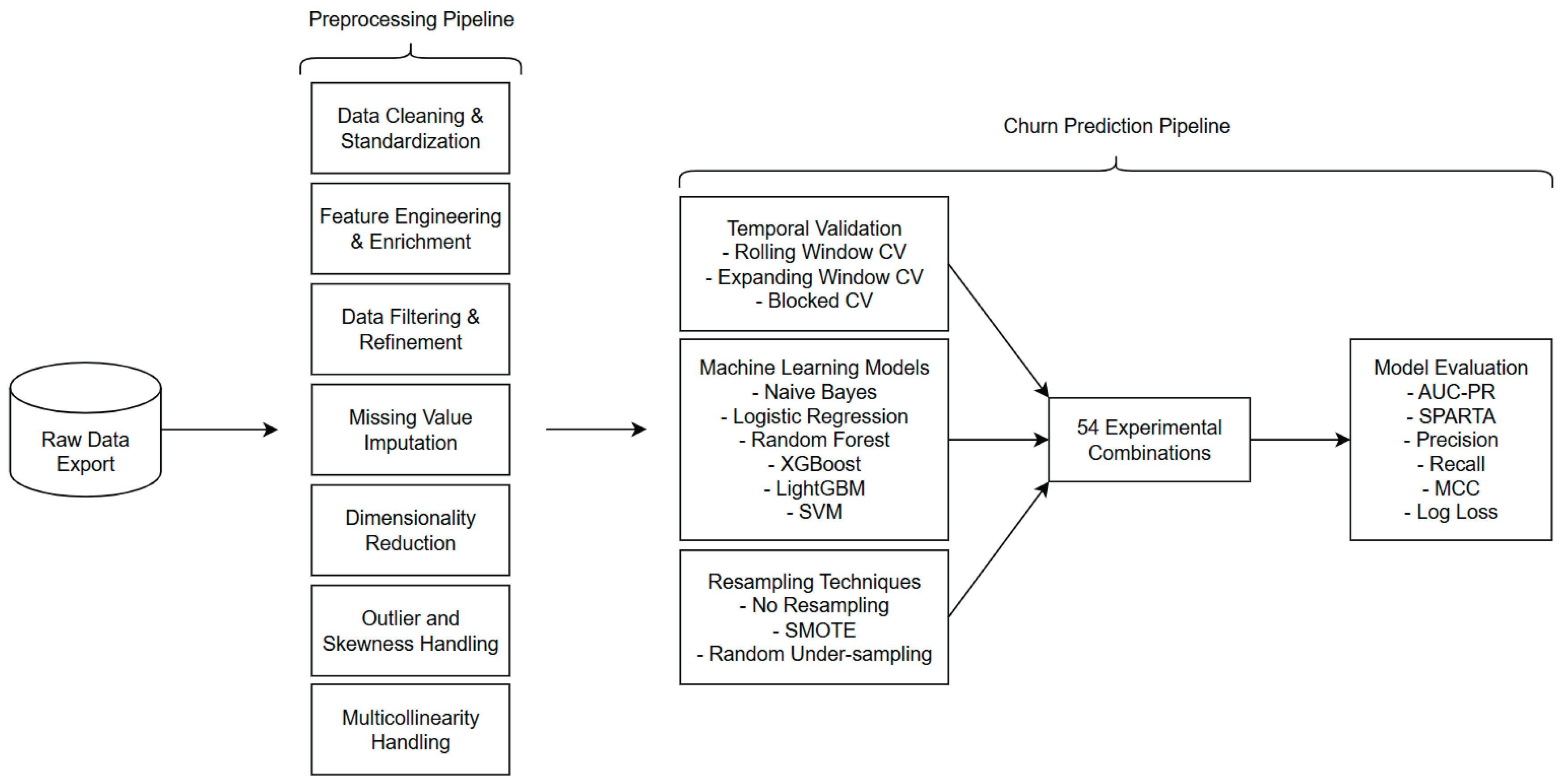
Figure 2.
Visualization of the Preprocessing Pipeline
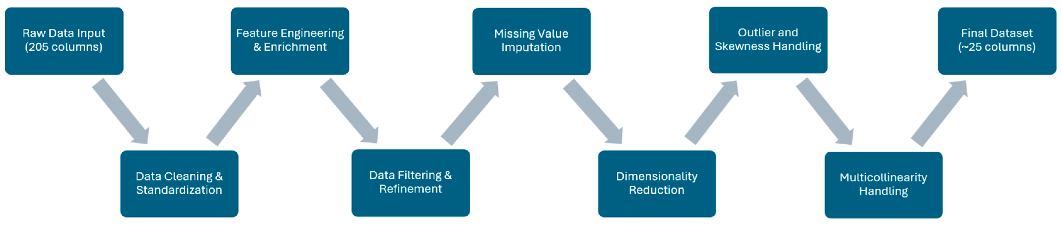
Figure 3.
Visualization of the employed Temporal Validation Strategies
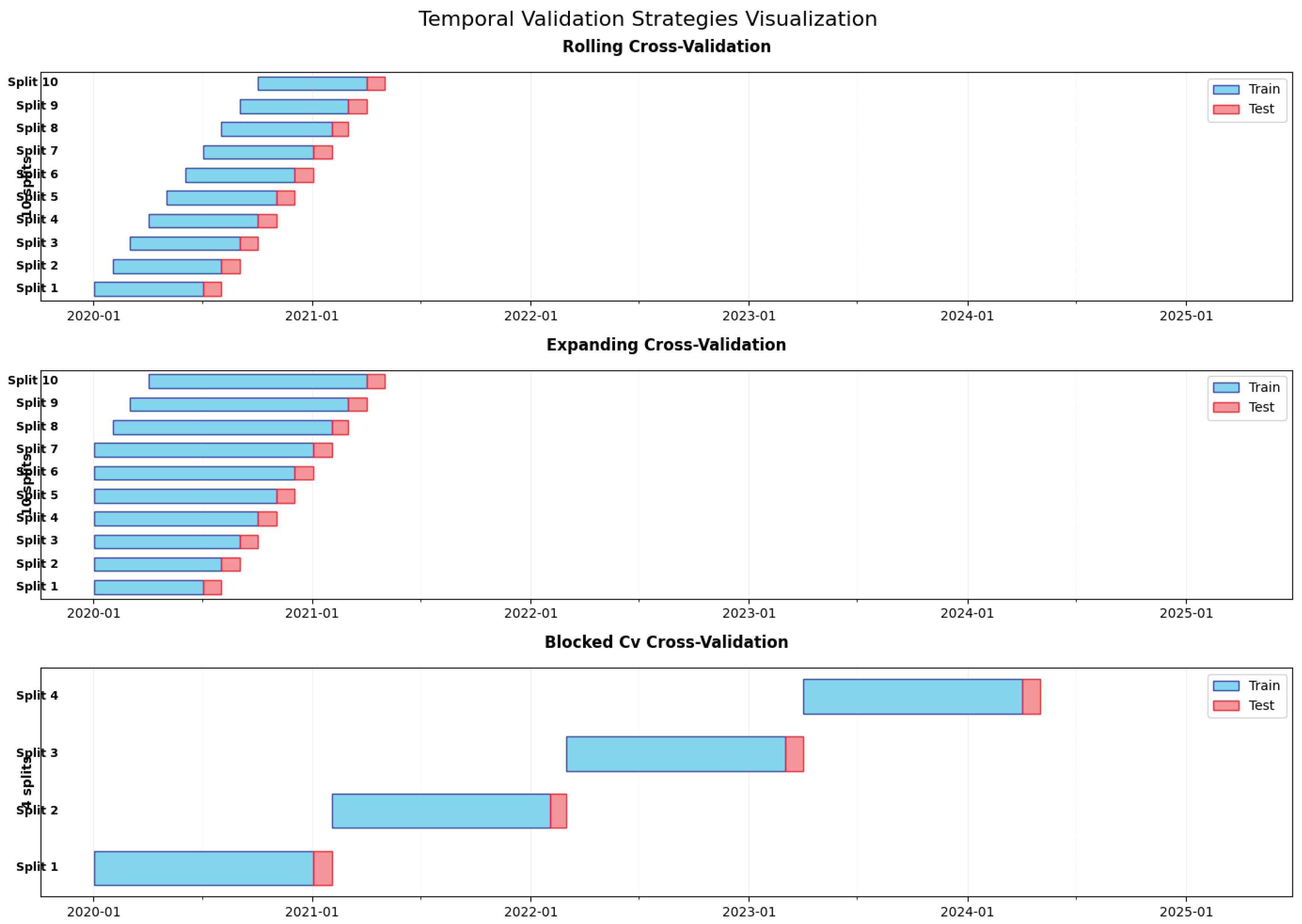
Figure 4.
Visualization of employed Resampling Methods.
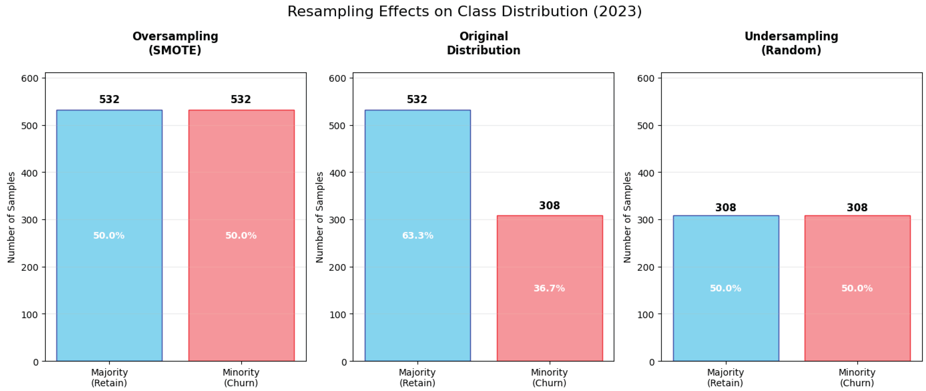

Table 3.1.
Top 10 Model Configurations by Mean AUC-PR.
| Rank | Model | Resampling | Temporal | AUC-PR | Std Dev | SPARTA | Stability |
| 1 | LightGBM | SMOTE | Blocked-CV | 0.99 | 0.013 | 0.948 | 0.944 |
| 2 | LightGBM | None | Rolling | 0.964 | 0.095 | 0.816 | 0.83 |
| 3 | LightGBM | None | Expanding | 0.96 | 0.101 | 0.816 | 0.83 |
| 4 | LightGBM | SMOTE | Rolling | 0.958 | 0.058 | 0.93 | 0.901 |
| 5 | LightGBM | SMOTE | Expanding | 0.955 | 0.059 | 0.921 | 0.896 |
| 6 | XGBoost | SMOTE | Expanding | 0.948 | 0.081 | 0.909 | 0.876 |
| 7 | LightGBM | None | Blocked-CV | 0.947 | 0.058 | 0.745 | 0.82 |
| 8 | XGBoost | SMOTE | Rolling | 0.938 | 0.088 | 0.903 | 0.867 |
| 9 | XGBoost | SMOTE | Blocked-CV | 0.933 | 0.084 | 0.881 | 0.859 |
| 10 | Random Forest | None | Expanding | 0.849 | 0.178 | 0.792 | 0.767 |
Table 3.2.
Performance Metrics by Temporal Validation Method.
| Temporal | AUC-PR | AUC-PR CV | Precision | Precision CV | Recall | Recall CV | MCC | MCC CV |
| Rolling | 0.487 | 0.421 | 0.325 | 0.746 | 0.804 | 0.436 | 0.366 | 0.694 |
| Expanding | 0.487 | 0.402 | 0.325 | 0.751 | 0.802 | 0.438 | 0.363 | 0.676 |
| Blocked-CV | 0.482 | 0.258 | 0.316 | 0.286 | 0.801 | 0.118 | 0.35 | 0.287 |
Table 3.3.
Performance Summary by Model (Averaged).
| Model | AUC-PR | AUC-PR CV | Precision | Precision CV | Recall | Recall CV | MCC | MCC CV |
| Naive Bayes | 0.454 | 0.176 | 0.042 | 0.528 | 0.916 | 0.137 | 0.09 | 0.408 |
| Log. Reg. | 0.145 | 0.607 | 0.09 | 0.557 | 0.808 | 0.102 | 0.195 | 0.364 |
| Rand. Forest | 0.611 | 0.315 | 0.527 | 0.387 | 0.764 | 0.141 | 0.515 | 0.25 |
| XGBoost | 0.55 | 0.326 | 0.527 | 0.272 | 0.839 | 0.206 | 0.502 | 0.248 |
| LightGBM | 0.696 | 0.264 | 0.589 | 0.299 | 0.918 | 0.121 | 0.625 | 0.24 |
| SVM | 0.48 | 0.461 | 0.226 | 1.416 | 0.581 | 1.234 | 0.278 | 1.703 |
Table 3.4.
Impact of Resampling Methods on Key Metrics.
| Resampling | AUC-PR | AUC-PR CV | Precision | Precision CV | Recall | Recall CV | MCC | MCC CV |
| None | 0.613 | 0.301 | 0.318 | 1.042 | 0.736 | 0.728 | 0.386 | 0.922 |
| SMOTE | 0.683 | 0.204 | 0.586 | 0.282 | 0.785 | 0.158 | 0.55 | 0.244 |
| Rand. Und. | 0.183 | 0.566 | 0.062 | 0.533 | 0.875 | 0.172 | 0.147 | 0.552 |
Table 3.5.1.
Top 5 Configurations for Company 1.
| Rank | Model | Resampling | Temporal | AUC-PR | SPARTA | Precision | Recall |
| 1 | LightGBM | SMOTE | Blocked-CV | 0.991 | 0.951 | 1 | 0.835 |
| 2 | LightGBM | None | Rolling | 0.951 | 0.763 | 0.662 | 0.999 |
| 3 | LightGBM | None | Expanding | 0.937 | 0.759 | 0.656 | 0.999 |
| 4 | XGBoost | SMOTE | Expanding | 0.906 | 0.871 | 0.969 | 0.642 |
| 5 | LightGBM | SMOTE | Rolling | 0.898 | 0.862 | 0.978 | 0.593 |
Table 3.5.2.
Top 5 Configurations for Company 2.
| Rank | Model | Resampling | Temporal | AUC-PR | SPARTA | Precision | Recall |
| 1 | LightGBM | SMOTE | Rolling | 0.988 | 0.971 | 0.991 | 0.923 |
| 2 | LightGBM | SMOTE | Expanding | 0.988 | 0.969 | 0.991 | 0.918 |
| 3 | LightGBM | SMOTE | Blocked-CV | 0.984 | 0.962 | 1 | 0.875 |
| 4 | LightGBM | None | Blocked-CV | 0.984 | 0.797 | 0.709 | 1 |
| 5 | XGBoost | SMOTE | Expanding | 0.972 | 0.935 | 0.99 | 0.804 |
Table 3.5.3.
Top 5 Configurations for Company 3.
| Rank | Model | Resampling | Temporal | AUC-PR | SPARTA | Precision | Recall |
| 1 | LightGBM | SMOTE | Blocked-CV | 0.994 | 0.932 | 0.992 | 0.793 |
| 2 | LightGBM | None | Blocked-CV | 0.993 | 0.778 | 0.683 | 1 |
| 3 | LightGBM | None | Expanding | 0.991 | 0.869 | 0.813 | 1 |
| 4 | LightGBM | SMOTE | Expanding | 0.989 | 0.954 | 0.994 | 0.863 |
| 5 | LightGBM | SMOTE | Rolling | 0.988 | 0.956 | 0.991 | 0.874 |
Table 3.6.
Average Training Time Per Split By Model and Configuration.
| Model | No Resampling (s) | SMOTE (s) | Random Under. (s) | Avg Split Time (s) |
| Naive Bayes | 0.15 | 0.18 | 0.15 | 0.16 |
| Logistic Reg. | 20.99 | 31.68 | 0.92 | 17.86 |
| Random Forest | 2.37 | 2.83 | 1.87 | 2.36 |
| XGBoost | 0* | 4.19 | 1.98 | 3.09 |
| LightGBM | 5.4 | 6.57 | 3.06 | 5.01 |
| SVM | 3.77 | 10.85 | 0.3 | 4.97 |
* All configs for XGBoost with No Resampling failed (see 3.7. Failed Experiments).
Table 3.7.1.
Individual Failed Experimental Configurations.
| # | Company | Model | Resampling | Temporal | Description |
| 1 | Company 1 | XGBoost | None | Blocked-CV | No successful splits processed |
| 2 | Company 1 | XGBoost | None | Expanding | No successful splits processed |
| 3 | Company 1 | XGBoost | None | Rolling | No successful splits processed |
| 4 | Company 2 | XGBoost | None | Blocked-CV | No successful splits processed |
| 5 | Company 2 | XGBoost | None | Expanding | No successful splits processed |
| 6 | Company 2 | XGBoost | None | Rolling | No successful splits processed |
| 7 | Company 3 | XGBoost | None | Blocked-CV | No successful splits processed |
| 8 | Company 3 | XGBoost | None | Expanding | No successful splits processed |
| 9 | Company 3 | XGBoost | None | Rolling | No successful splits processed |
Table 3.7.2.
Summary of Failed Experiments by Configuration Components.
| Component | Category | Total Configs | Failed Configs | Failure Rate (%) |
| Company | Company 1 | 54 | 3 | 5.6 |
| Company | Company 2 | 54 | 3 | 5.6 |
| Company | Company 3 | 54 | 3 | 5.6 |
| Model | Naive Bayes | 27 | 0 | 0 |
| Model | Logistic Reg. | 27 | 0 | 0 |
| Model | Random Forest | 27 | 0 | 0 |
| Model | XGBoost | 27 | 9 | 33.3 |
| Model | LightGBM | 27 | 0 | 0 |
| Model | SVM | 27 | 0 | 0 |
| Resampling | None | 54 | 9 | 16.7 |
| Resampling | SMOTE | 54 | 0 | 0 |
| Resampling | Random Under. | 54 | 0 | 0 |
| Temporal | Rolling | 54 | 3 | 5.6 |
| Temporal | Expanding | 54 | 3 | 5.6 |
| Temporal | Blocked-CV | 54 | 3 | 5.6 |
Disclaimer/Publisher’s Note: The statements, opinions and data contained in all publications are solely those of the individual author(s) and contributor(s) and not of MDPI and/or the editor(s). MDPI and/or the editor(s) disclaim responsibility for any injury to people or property resulting from any ideas, methods, instructions or products referred to in the content. |
© 2025 by the authors. Licensee MDPI, Basel, Switzerland. This article is an open access article distributed under the terms and conditions of the Creative Commons Attribution (CC BY) license (http://creativecommons.org/licenses/by/4.0/).
Copyright: This open access article is published under a Creative Commons CC BY 4.0 license, which permit the free download, distribution, and reuse, provided that the author and preprint are cited in any reuse.


