
Submitted:
11 December 2025
Posted:
12 December 2025
You are already at the latest version
Abstract
This study examines the impact of increasing photovoltaic (PV) penetration on the transient stability of the IEEE 9-bus power system. Synchronous machines are modeled with standard subtransient dynamics, while PV units are represented as current-limited grid-following inverters. Transient stability is assessed through the Critical Clearing Time (CCT) and the post-fault dynamic behavior, obtained from time-domain simulations carried out in MATLAB/Simulink®. A permanent three-phase fault on line 7–5 is considered as the limiting contingency. The results show an increase in CCT as PV generation progressively replaces the active power supplied by synchronous machines, whose inertia is therefore maintained: from 210 ms (0% PV) to 440 ms (25%) / 1080 ms (40%) at bus 5, 410 ms (25%) / 1130 ms (40%) and 290 ms (25%) / 650 ms (40%) at buses 6 and 8, respectively, demonstrating that the injection site is a key factor for system stability. For distributed injection among the three buses, CCT values of 340 ms (25%) and 1020 ms (40%) highlight the significant influence of PV placement at bus 8. Although an overall increase in CCT was observed, higher PV penetration also led to more pronounced oscillations and operability issues after the fault. These results underscore the need for stability-oriented control strategies, such as grid-forming operation, fast active power support, and dynamic voltage control. They also suggest that planning practices should favor interconnections electrically closer to the slack generator. Overall, a high PV penetration level—modifying only the operating point of synchronous machines—allows longer fault durations to be tolerated; however, appropriate siting of PV units and the adoption of advanced inverter controls could mitigate the observed oscillations and post-fault operability challenges.
Keywords:
Critical Clearing Time (CCT)
; electrical power system
; PV penetration
; transient stability
; IEEE 9-bus power system
1. Introduction
Renewable energy sources (RES) are integrated into conventional electrical power systems (EPS) to solve issues like fossil fuel shortages, rising energy demand, and environmental pollution [1]. Among the alternative RES, solar photovoltaic (PV) systems are now a well-established option due to their simple design and low capital and operational costs. It is also notable that, worldwide, total PV capacity has increased at an average annual rate of 55% [2]. These factors have made PV technology an attractive option for power generation and a central focus of ongoing research in modern power systems.
PV systems can generally be classified into two main categories: isolated and connected to the grid, the latter being the ones that have been widely adopted. Although PV renewable energy brings clear environmental advantages, its integration also alters the operational and dynamic characteristics of electrical power systems compared to conventional networks [3]. Unlike synchronous generators, inverter-based renewable units do not store kinetic energy in a rotating mass and therefore cannot inherently contribute to the inertial response of the system. Their interaction with the grid occurs through power-electronic converters, whose current and control limitations reduce the system’s effective inertia and weaken the synchronizing torque. As a consequence, the ability of the network to withstand and mitigate disturbances can be significantly affected, and the transient stability margin may be compromised [4].
The need to integrate renewable energy sources with high penetration, driven by the energy transition and the major advances in power electronics, has become a central research topic due to the new network configurations and the different responses they exhibit under various disturbances. Numerous studies have been conducted in this field and have highlighted both positive and negative effects associated with high PV penetration in EPS.
In the study presented in [5], the authors reported that, due to the stochastic nature of PV systems, issues such as voltage and frequency fluctuations, active power variations, reactive power flow changes, and degraded system dynamics may arise as a consequence of irradiation variations caused by the rapid and constant movement of clouds. Factors such as the size and location of PV systems, whether they are distributed or concentrated, the availability of sufficient reserves in the system, the displacement of conventional generators by PV production, the reactive power compensation method, and the control loops influence the impact of PV penetration on the EPS with respect to voltage stability, frequency stability, and transient stability [6].
Conversely, the authors in [7] observed that high PV penetration affects the angle and frequency stability of the transmission system. In [8], the transient stability of large-scale PV systems integrated into the Ontario network was examined. Their results indicate that transient stability improves more with distributed PV penetration than with concentrated PV. The effect of PV systems installed on residential rooftops was analyzed in [9] with respect to the transient stability of an interconnected grid in the western United States. The findings suggest that increasing PV penetration deteriorates transient stability due to the reduction of system inertia; however, when faults occur in less critical locations, transient stability can improve. Finally, the authors investigated the effect of different levels of PV penetration on rotor angle stability in the standard IEEE 9-bus test system, described in [10], and found that increasing PV penetration improves transient stability when the synchronous generator is not replaced. When it is replaced, system stability decreases. They ultimately concluded that the key factors influencing transient stability in an EPS are the PV penetration level, the fault clearing time, and the fault location.
In summary, this literature review shows that the behavior of the power system under high PV penetration depends strongly on how this penetration is implemented. An improvement in transient stability is generally observed when the synchronous generator is not replaced and synchronous inertia remains constant, highlighting the complexity of understanding these systems and the need for further research. Despite the variety of studies in the field, few investigations focus on the post-fault behavior of systems, particularly in cases where PV penetration does not negatively affect transient stability. In scenarios where the CCT increases with penetration level, understanding the post-fault dynamic behavior of the system becomes important to ensure that transient stability is not adversely affected in practice.
This article conducts simulations to evaluate the transient stability of the IEEE 9-bus system under different levels of PV penetration. The main objective is to determine the Critical Clearing Time (CCT), considering the geographical location of the injections and the various injection typologies. Here, injection refers to the active power supplied by PV systems that is incorporated into the EPS.
More specifically, the work consists of:
- Developing a detailed simulation model of the IEEE 9-bus system for transient stability studies, comprising three synchronous generators and current-limited grid-following inverters representing PV units connected at buses 5, 6, and 8. PV penetration levels of 25% and 40% were implemented using MATLAB/Simulink®.
- Considering a permanent three-phase fault on line 7–5 of the network. The computation of the CCT and the analysis of the post-fault dynamic behavior were carried out for each level of PV penetration, including both distributed and concentrated injection scenarios, in which the synchronous generators are not replaced (constant synchronous inertia).
The main contributions of this research are as follows:
- Precise indicators, such as the CCT, enabling the characterization of network behavior with PV integration under transient stability conditions.
- Quantitative information allowing comparison of system performance depending on the injection location and topology.
- An analysis of the post-fault dynamic behavior, enabling the assessment of whether the system meets operability requirements in each scenario.
These results are highly valuable for network operators integrating renewable energy sources, as they support improved planning and more accurate configuration of protection relays. They also represent a significant scientific contribution by enabling further and more detailed studies on this topic.
2. Materials and Methods
2.1. Transient Stability Criterion
The dynamics in EPS can be categorized into three types: electromagnetic, electromechanical, and steady-state. Small, gradual changes in the EPS are considered minor disturbances, and studying stability within this domain is known as small-signal stability. Large disturbances, such as the disconnection of gas loads or large generators, the rupture of transmission lines or link lines, and short circuits, relate to the concept of transient stability, which is defined as the ability of the EPS to remain synchronized under large disturbances. During such events, transient stability analysis helps determine the deviation behavior of the rotor angle. If these disturbances are not removed within a specified time, they can cause generators to lose synchronism, potentially leading to the disconnection of the entire system.
To study transient stability, various indicators can be examined, including rotor velocity deviation, rotor angle, frequency, voltage at the generator terminals, and the CCT of faults [11]. The CCT is defined as the maximum time available to eliminate a fault while maintaining system stability [12]. A higher CCT means more time to clear faults, making the system safer. An important factor in stability studies is the power dynamics over different time scales. For a conventional EPS based on synchronous generators, the dynamic time frame ranges from a few seconds, while for RES it is studied over a longer period, up to several seconds [13]. Achieving transient stability in an EPS requires generators to remain synchronized, keeping the stability indicators within acceptable limits. However, the CCT value depends on factors such as generator size, inertia, dispatch conditions, line impedances, network topology, fault location, and other transient stability-related aspects. Additionally, weather conditions can also influence the transient stability of multiple machines.
2.2. Dynamic Models of Synchronous Generators
After exposing the EPS to a 3 failure, the transient stability is analyzed using the oscillation equation described in (1),
where H [s] is the inertia constant, defined as the resistance of the rotating masses coupled to the generators against any change in the speed or direction of rotation, which depends on the kinetic energy and the system capacities. It is defined as the ratio between the kinetic energy [MJ] at nominal speed and the machine rating [MVA]. [Hz] is the system frequency, [rad] is the angular displacement of the electrical power, [p.u.] is the mechanical power (per unit) of the prime mover, and [p.u.] is the electrical power delivered (per unit). When is expressed in degrees, the equation becomes:
After the EPS experiences a disturbance, the transient stability is analyzed by solving the nonlinear oscillation equation within 3 to 5 seconds (where ). The electrical power produced is then calculated as:
where E is the constant internal voltage behind the synchronous reactance (per unit), V is the load voltage of the infinite bus (per unit), and X is the steady-state reactance between the generator and the bus. From the curve of the angular displacement of power, shown in Figure 1, the maximum power delivered occurs at , as indicated in Equation (4).
Note that when , the EPS is stable, while if , the EPS is unstable. At , the generator is considered marginally stable, so any further increase in the angle makes the EPS unstable.
The equation described in (1) allows us to study the rotor angle behavior of a single generator; however, the system used in this research is a multi-machine system consisting of 3 generators supplying 3 loads. For a multi-machine system composed of N generators, N swing equations are defined as in Equation (5), with the electrical power of machine i given by Equation (6). The system therefore contains N solutions that make it possible to determine the transient stability of the multi-machine system. Due to their complexity, numerical methods are often used to solve these equations.
2.3. Modelling of the PV Systems
A PV system consists of cells connected in series that form a module. Different models are used for PV cells to produce accurate results [17]. Figure 2 shows the equivalent circuit of a diode model of a PV cell.
Applying basic electrical engineering techniques, such as Kirchhoff’s current law (KCL) and other methods detailed in [18], the output current of the PV cell, denoted by I, is determined as follows:
where is the current generated in the cell due to solar irradiance, is the diode current governed by the Shockley equation shown in (8), and is the current representing cell losses as expressed in (9). is the diode saturation current, n is the diode ideality factor, and are the series and parallel resistances used in the diode equivalent circuit, respectively. is the thermal voltage defined in (10), k is the Boltzmann constant (), is the cell temperature, and q is the electron charge.
Therefore, Equation (7) becomes:
where and represent the module voltage and current, respectively; , , and denotes the number of cells connected in series in the PV module.
In this study, uniform irradiance and a consistent temperature are assumed for all cells in the modules and arrays. It is important to note that under fault conditions, PV systems behave differently from synchronous generators in conventional EPS. Due to the presence of interface inverters that connect PV systems (which generate DC) to loads (which require AC), their short-circuit currents are typically below 150% of the nominal current [19]. This is because inverters are equipped with modern protective current limiters designed to prevent high short-circuit currents and protect semiconductor switches.
To model the PV system, PV modules—each composed of multiple PV cells—are arranged in series and parallel to form a PV string with a nominal capacity of 6 MWp. This configuration is capable of delivering up to 6 MVA to the 230 kV three-phase network through power electronic converters. To extract the maximum power from the PV array, grid-following inverters are placed at the output of each string. A Perturbation and Observation (P&O) algorithm is used as the direct control strategy for the maximum power point tracking (MPPT) while operating in unity power factor mode ().
The DC/AC conversion is performed using a three-level Neutral Point Clamped (NPC) voltage source converter. The switching function of the converter is implemented with a model that is directly controlled by the reference voltage. Since the converter output voltage is 260 V, a step-up power transformer is connected downstream to match the grid voltage level. An RL filter is included at the converter output to ensure waveform quality and to protect both the network and the converter from high-frequency components.
The parameters of the PV string and converter system are listed in Table 1. Depending on the penetration level considered in the simulations, the system is duplicated and connected in parallel to supply the required power.
2.4. Description of the Proposed EPS
In this study, the IEEE 9-bus system [16] is modeled and analyzed using the MATLAB–Simulink® environment. Its main components include: 9 buses numbered from 1 to 9; 3 conventional generators (G1, G2, and G3) located at buses 1, 2, and 3 respectively; 3 transformers; 6 transmission lines of 100 km each; and 3 static loads located at buses 5, 6, and 8. The complex base power used for expressing the quantities in per unit is set to 100 MVA.
To perform the transient stability studies, detailed data for buses, generators and lines are required. The bus data for the test system are presented in Table 2 [10].
The slack (reference) bus has a predefined voltage magnitude and phase angle ( and ) of 1.04 p.u. and , respectively, while its active and reactive powers are determined from the load flow analysis. The generator (PV) buses have specified voltage magnitudes () and active power outputs (), whereas the corresponding reactive powers () and voltage angles () are obtained from the load flow results. Similarly, the remaining buses are considered as PQ (load) buses with defined real and reactive power demands, while their voltage magnitudes () and phase angles () are derived from the same analysis. The dynamic parameters of the three synchronous generators are listed in Table 3, and the line data are detailed in Table 4 [10]. The per-unit system is based on a 100 MVA power base.
2.5. Methodology
In this section, we present the methodological approach adopted to model and simulate an electric power system with two different levels of solar penetration, with the objective of assessing its transient stability. This approach clearly defines the goals of the study, the tools used, and the assumptions made to ensure that the simulation remains both realistic and exploitable.
The system is modeled in MATLAB/Simulink® and is based on the IEEE 9-bus system, which includes three conventional generators, three transformers, six transmission lines of 100 km each, and three static loads. For the penetration levels, two scenarios are considered, in accordance to the following classification [14,15] :
- Moderate penetration level: 25%
- High penetration level: 40%
Solar penetration is introduced directly at the buses where loads are connected, and in two configurations: a concentrated injection at one of buses 5, 7, or 8, where the total PV power is injected at the selected bus; and a distributed injection across the three buses simultaneously, where the injected power is shared proportionally according to the load distribution at each bus, following Equation (12). The conventional generators are not replaced with smaller units under renewable energy injection scenarios. Instead, their operating power is reduced to prioritize renewable energy injection. The reduction on the PV side is also performed proportionally, following a formulation consistent with the proportionality of the load.
where: is the adjusted power of generator i; , the power of generator i in the reference case without PV penetration; , the total generated power in the reference system and the total active power injected by the PV systems.
For the transient stability study, a permanent three-phase symmetrical fault is applied, as it represents the most severe type of disturbance in an electric power system [10]. A permanent fault means that the line on which the disturbance occurs is removed from service after fault clearing. The fault location is chosen on the line closest to the largest PV generator, since disturbances near large generators typically produce stronger effects. Because transient stability phenomena occur over a short duration, all simulations are performed over a 7-second window, with the fault activated at s. The primary conditions of the PV system (irradiance, temperature) are assumed to remain constant during the simulation.
The Critical Clearing Time is used as the main indicator to determine the transient stability of the system by analyzing the rotor angle response of the generators following the disturbance. The CCT corresponds to the maximum duration during which a disturbance can persist without causing loss of synchronism.
A series of simulations is performed by progressively increasing the fault duration in 10 ms increments. The maximum fault duration that allows the system to remain stable is considered the CCT. An additional simulation is carried out using a fault duration 10 ms longer than the CCT, in order to illustrate the behavior of the unstable system. As a complementary analysis, the active power generated by the solar system is also presented to observe the dynamic response of the different sources before and after the system disturbance.
The different scenarios used for the study are considering a permanent three-phase symmetrical fault on transmission line 7–5 for the different levels of PV penetration determined as percentages using Equation (13) (0%, 25%, and 40%). In each case, except for the first, the injection is applied in a concentrated manner near the static loads at buses 5, 6, and 8, and then distributed uniformly among these three buses. In this situation, the distribution of PV power follows the same pattern as that of the static loads.
3. Results and Discussion
3.1. Reference Case (0% PV)
To evaluate the transient stability of the IEEE 9-bus system, a permanent three-phase fault was applied on transmission line 7–5, following the methodology outlined in Section 2.5. The time-domain simulation shows that, for a fault duration of 210 ms, all three synchronous generators remain stable after the clearance of the disturbance. However, when the fault duration is increased to 220 ms, the system is no longer able to return to a stable post-fault operating condition.
Accordingly, the CCT of the reference case (without renewable energy injection) is estimated at 210 ms. This value serves as the baseline for all subsequent scenarios analyzed in this study.
Figure 5 illustrates the rotor angle trajectories of the three generators. For a 210 ms fault, the rotor angles reconverge within approximately three seconds after the disturbance is cleared, indicating a stable post-fault response. In contrast, for a 220 ms fault, the rotor angles exhibit persistent oscillations and diverge with time, demonstrating a loss of synchronism and confirming instability.
3.2. Impact of PV Penetration on the CCT
As described in Section 2.5, the same permanent three-phase fault is applied to the modified power system for all PV penetration levels. Table 7 presents the CCT values obtained for each simulated scenario, illustrating the impact of photovoltaic penetration on the transient stability of the system.
In general, photovoltaic injection has a positive impact on the CCT for all penetration levels and topologies, as long as the synchronous generators remain in service and the system inertia is preserved. The increase in CCT values is explained by the reduction in the mechanical power supplied by each synchronous generator, which decreases the rotor acceleration during the fault . As a result, the rotor angle evolves more slowly, allowing the system to withstand longer fault durations before losing synchronism.
Although the overall effect is positive, the injection location also plays an important role in determining system robustness. For concentrated injections, PV penetration at bus 8 consistently yields the lowest CCT values, regardless of the penetration level (see lines 1–3 in Table 7). This can be attributed to the fact that bus 8 is electrically the farthest from the slack bus, leading to a weaker synchronizing coupling with the system reference. In other words, the higher electrical distance to the slack generator increases the sensitivity of bus 8 to rotor angle deviations during the disturbance, thereby reducing the transient stability margin.
For distributed injections, the robustness of the system improves (line 4 of Table 7) compared with the concentrated injection at bus 8 (line 3). However, it remains lower than the robustness obtained when PV is concentrated at buses 5 or 6 (lines 1 and 2). This behavior can be explained by the fact that a non-negligible portion of the distributed PV power is still injected at bus 8, which continues to weaken the global synchronizing strength of the system, even though distribution mitigates part of the negative effect associated with this injection point.
The simulations also reveal that the increase in CCT between the two penetration levels is not linear, regardless of the injection topology. This strong variation arises because the rotor equation described in Equation (1) does not produce a linear response with respect to the mechanical power input. A reduction in leads to a rapid decrease in the accelerating power , which significantly modifies the stability behavior of the machine. As a result, the system shifts into a more favorable stability region, causing a disproportionate increase in CCT as PV penetration rises from 25% to 40%.
3.3. Post-Fault Dynamic Behavior
3.3.1. Rotor Angle Dynamics
The increase in CCT values observed in the previous section suggests a more robust system when subjected to severe disturbances. However, the analysis of post-fault behaviors shows that the rotor angles exhibit oscillations of larger amplitude compared to the reference case, and of longer duration.
These prolonged oscillations are explained by the reduction in mechanical power supplied by the synchronous machines, a direct consequence of the partial replacement of conventional generation by photovoltaic generation. With lower mechanical power available, rotor acceleration is reduced, leading to slower damping and a delayed recovery of the system after fault clearance.
Despite this slower dynamic response, these cases are still considered stable. According to the literature, for small power systems such as the IEEE 9-bus system, the rotor angles must show a clear tendency to return toward a synchronized trajectory within 3 to 5 seconds following the fault clearance [20].
3.3.2. Active Power Dynamics
The analysis of active power provides a key indicator of the system’s operational capability following a disturbance. Among the existing standards governing the interconnection of renewable energy sources to the electric grid, IEEE 1547-2018 and IEEE 2800-2022 specify, through precise thresholds and time requirements, that renewable energy sources should not disconnect unnecessarily and must support the grid during and after a disturbance [21,22]. This section examines the obtained results to assess compliance with these requirements.
25% PV Penetration
Concentrated injections:
- Bus 5: The active power exhibits oscillations after fault clearing and stabilizes within approximately 2 s, meeting the normative requirements.
- Bus 6: The power also oscillates but fails to reach 90% of its nominal value within the 2 s required by the standards, representing an operability issue.
- Bus 8: The injected power stabilizes immediately after fault clearing.
In all three cases, the PV system remains connected, in accordance with LVRT requirements. The observed oscillations are primarily driven by the dynamics of synchronous generators, as PV inverters operate in grid-following mode.
Distributed injection: The active power injected at buses 5 and 6 shows behavior similar to that of the concentrated cases. However, at bus 8, the power does not stabilize within the required time window, also indicating a lack of operational compliance. With two out of three sites failing to meet the requirements, the system exhibits operability limitations for this level of distributed penetration.
40% PV Penetration
Concentrated injections:
- Bus 5 and Bus 6: Active power oscillates after the disturbance but stabilizes within the required timeframe.
- Bus 8: Oscillations persist and eventually lead to loss of synchronism and disconnection, highlighting a major operability issue.
Distributed injection: All three injection sites exhibit non-compliant dynamic behavior relative to the normative criteria, indicating that the system is unable to satisfy operability requirements at this penetration level.
4. Conclusions
This study aimed to evaluate the impact of high PV penetration on the transient stability of the IEEE 9-bus system using MATLAB/Simulink®. The results showed that, in terms of transient stability, PV injection increases the CCT when synchronous inertia remains constant. The injection location and topology strongly influence system robustness, with Bus 8 identified as the most critical injection point for all penetration levels.
The post-fault dynamic behavior exhibited rotor angle oscillations and, in some cases, operability issues, particularly when the technical requirements of IEEE 1547 and IEEE 2800 were not met. These findings highlight the importance of planning strategies that consider the PV injection location as well as detailed post-fault behavior to ensure operational compliance of the network.
However, the study relies on a reduced 9-bus system and grid-following converters. Therefore, the conclusions should be interpreted as indicative trends regarding the dynamic behavior of a real system, and more comprehensive analyses are required for broader generalization. The introduction of grid-forming converters could also modify the conclusions obtained.
Future work may include the study of hybrid PV+BESS technologies and the use of more complex networks such as the IEEE 14-bus or IEEE 32-bus systems.
Author Contributions
Conceptualization, M.J.P.; methodology, M.J.P.; software, M.J.P.; validation, E.H.M. and O.R.R.; formal analysis, M.J.P.; investigation, M.J.P.; resources, E.H.M., O.R.R. and O.A.J.; data curation, M.J.P.; writing—original draft preparation, M.J.P.; writing—review and editing, E.H.M., O.R.R. and O.A.J.; visualization, M.J.P.; supervision, E.H.M. and O.A.J.; project administration, E.H.M. All authors have read and agreed to the published version of the manuscript.
Funding
This research received no external funding.
Acknowledgments
The authors thank the Instituto de Energías Renovables (IER–UNAM) for technical support and resources used during simulation development.
Conflicts of Interest
The authors declare no conflict of interest. The funders had no role in the design of the study; in the collection, analyses, or interpretation of data; in the writing of the manuscript; or in the decision to publish the results.
References
- IRENA. Renewable Power Generation Costs in 2022; International Renewable Energy Agency: Abu Dhabi, 2023. [Google Scholar]
- Pessanha, J.; Melo, A.; Caldas, R.; Falcao, D. An approach for data treatment of solar photovoltaic generation. IEEE Lat. Am. Trans. 2020, 18, 1563–1571. [Google Scholar] [CrossRef]
- Šešok, A.; Pavić, I. Transient stability improvement of Croatian power system using FACTS. In Proceedings of the 11th International Conference on Innovative Smart Grid Technologies—Asia (ISGT-Asia 2022), 2022; IEEE: Singapore. [Google Scholar] [CrossRef]
- Lopes, J.C.; Sousa, T. Transmission system electromechanical stability analysis with high penetration of renewable generation and battery energy storage system application. Energies 2022, 15, 62060. [Google Scholar] [CrossRef]
- Wandhare, R.G.; Agarwal, V. Novel stability enhancing control strategy for centralized PV-grid systems for smart grid applications. IEEE Trans. Smart Grid 2014, 5, 1389–1396. [Google Scholar] [CrossRef]
- Shah, R.; Mithulananthan, N.; Bansal, R.; Ramachandaramurthy, V. A review of key power system stability challenges for large-scale PV integration. Renew. Sustain. Energy Rev. 2015, 41, 1423–1436. [Google Scholar] [CrossRef]
- Achilles, S.; Bebic, S. Transmission system performance analysis for high penetration photovoltaics; National Renewable Energy Laboratory (NREL): Golden, CO, USA, 2008. Report No. SR-581-42300.
- Tamimi, B.; Canizares, C.; Bhattacharya, K. System stability impact of large scale and distributed solar photovoltaic generation: The case of Ontario. IEEE Trans. Sustain. Energy 2013, 4, 680–688. [Google Scholar] [CrossRef]
- Eftekhari-Nejad, S.; Vittal, V.; Heydt, G.T.; Loehr, K. Impact of increased penetration of photovoltaic generation on power system. IEEE Trans. Power Syst. 2013, 28, 893–901. [Google Scholar] [CrossRef]
- Kamel, R.M.; Alanzi, S.S.; Hashemi, Y.M.A. Effect of photovoltaic penetration level and location on power system transient stability during symmetrical and unsymmetrical faults. Sustain. Energy Grids Netw. 2024, 38, 101322. [Google Scholar] [CrossRef]
- Mazhari, S.M.; Safari, N.; Chung, C.Y.; Kamwa, I. A Hybrid Fault Cluster and Thevenin Equivalent Based Framework for Rotor Angle Stability Prediction. IEEE Trans. Power Syst. 2018, 33, 5594–5603. [Google Scholar] [CrossRef]
- Sharma, R.; Singh, M.; Jain, D.K. Power System Stability Analysis with Large Penetration of Distributed Generation. In Proceedings of the 6th IEEE Power India Conference, Delhi, India, 5–7 December 2014; IEEE; pp. 1–6. [Google Scholar] [CrossRef]
- Barbosa, D.M.; Kuiava, R.; Piazza, T.S. Transient Stability Constrained Optimal Power Flow Applied to Distribution System with Synchronous Generators. IEEE Lat. Am. Trans. 2022, 20(2), 335–343. [Google Scholar] [CrossRef]
- De Witt, W.; García, M.; López, R. Classification of Renewable Energy Penetration Levels in Modern Power Systems. Int. J. Renew. Energy Res. 2021, 11(2), 987–995. [Google Scholar]
- Muhando, B.; Keith, K.; Holdmann, G. Power Electronics Review—Evaluation of the Ability of Inverters to Stabilize High-Penetration Wind–Diesel Systems in Diesel-Off Mode Using Simulated Components in a Test Bed Facility; Alaska Center for Energy and Power: Fairbanks, AK, USA, 2010.
- Loji, K.; Loji, N.; Kabeya, M. Flexibility Assessment of a Solar PV Penetrated IEEE 9-Bus System Using Dynamic Transient Stability Evaluation. In Proceedings of the 2022 IEEE PES/IAS Power Africa Conference, Kigali, Rwanda, 2–6 August 2022; pp. 1–5. [Google Scholar] [CrossRef]
- Montano, J.J.; Grisales, L.F.; Tobon, A.F.; González, D. Estimation of the parameters of the mathematical model of an equivalent diode of a photovoltaic panel using a continuous genetic algorithm. IEEE Lat. Am. Trans. 2022, 20, 616–623. [Google Scholar] [CrossRef]
- Cervellini, M.P.; Echeverria, N.I.; Antonszczuk, P.D.; Retegui, R.A.G.; Funes, M.A.; González, S.A. Optimized parameter extraction method for photovoltaic devices model. IEEE Lat. Am. Trans. 2016, 14, 1959–1965. [Google Scholar] [CrossRef]
- Brito, M.; Alves, M.; Canesin, C. Microgrid system with emulated PV sources for parallel and intentional islanding operations. IEEE Lat. Am. Trans. 2020, 18, 1462–1469. [Google Scholar] [CrossRef]
- Kundur, P. Power System Stability and Control; McGraw–Hill: New York, NY, USA, 1994. [Google Scholar]
- IEEE Std 1547-2018; IEEE Standard for Interconnection and Interoperability of Distributed Energy Resources with Associated Electric Power Systems Interfaces. IEEE: New York, NY, USA, 2018.
- IEEE Std 2800-2022; IEEE Standard for Interconnection and Interoperability of Inverter-Based Resources with Associated Transmission Electric Power Systems. IEEE: New York, NY, USA, 2022.
Figure 1.
Power angular displacement curve for typical EPS.
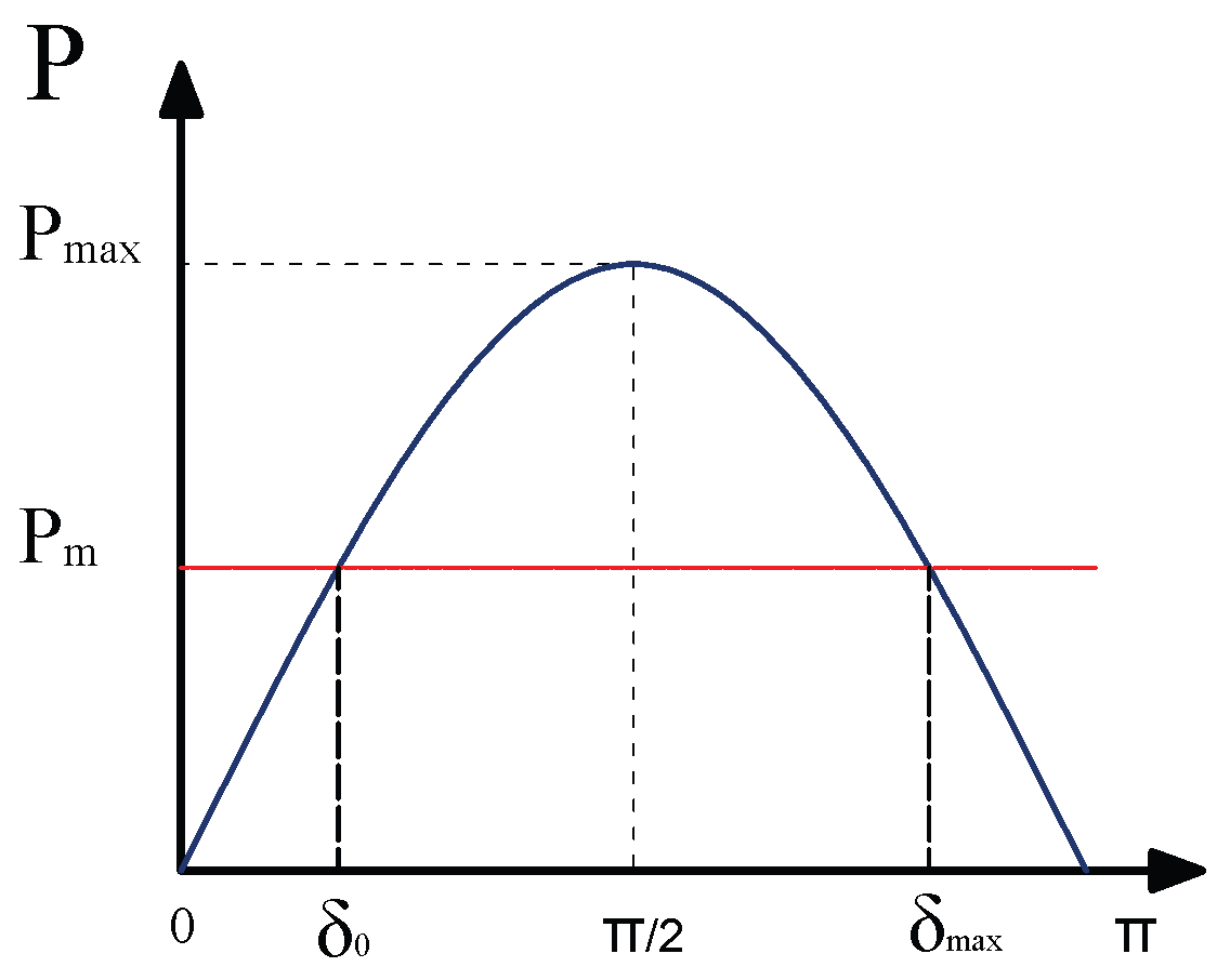
Figure 2.
Single-line diagram of the 9-bus system with the fault.
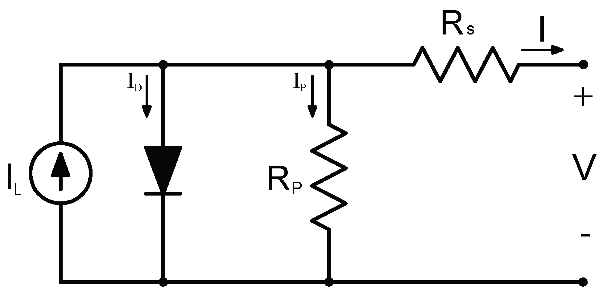
Figure 3.
Single-line diagram of the 9-bus system with the fault.
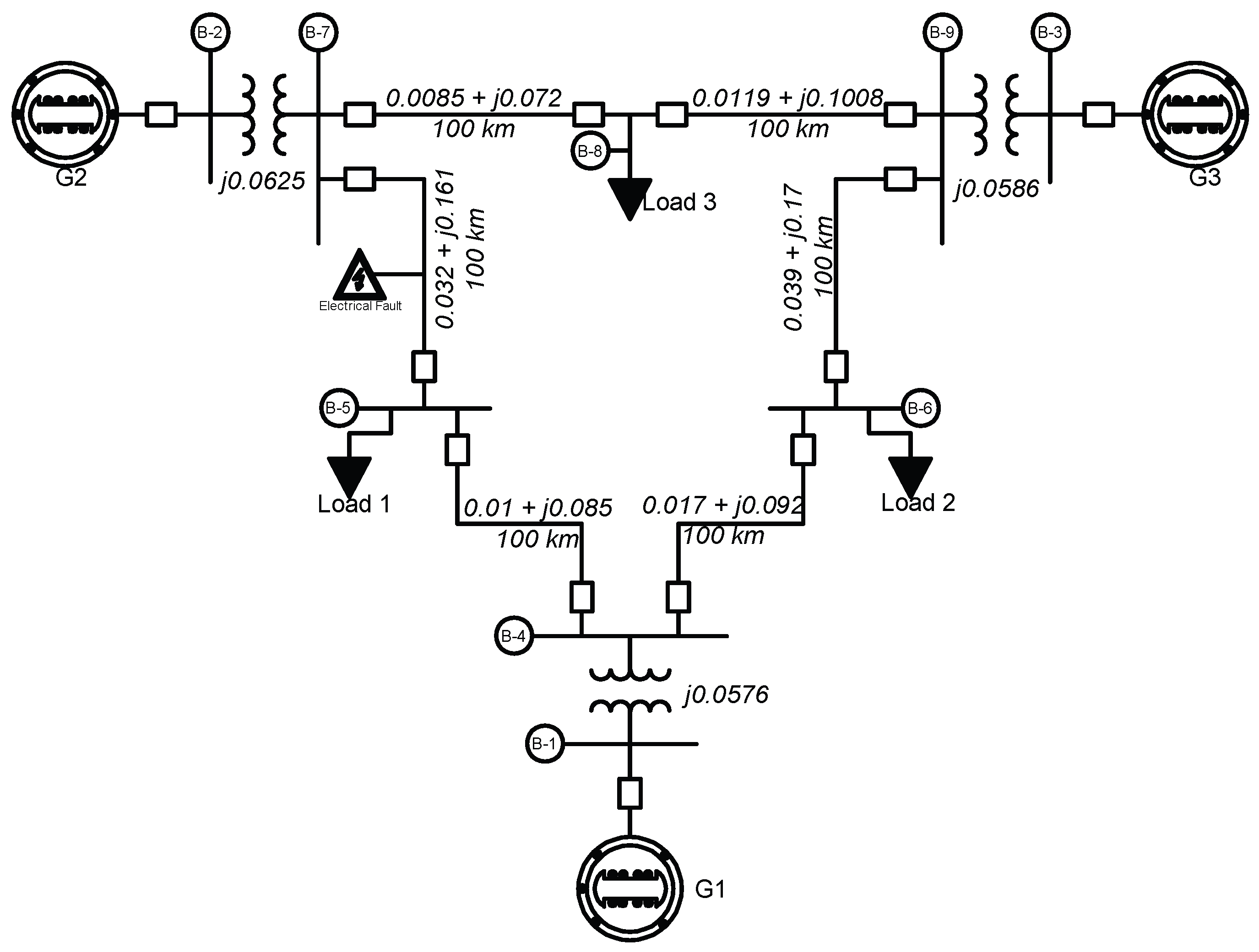
Figure 4.
Single-line diagram of the 9-bus system with the fault and PV distributed across the three buses.
Figure 4.
Single-line diagram of the 9-bus system with the fault and PV distributed across the three buses.
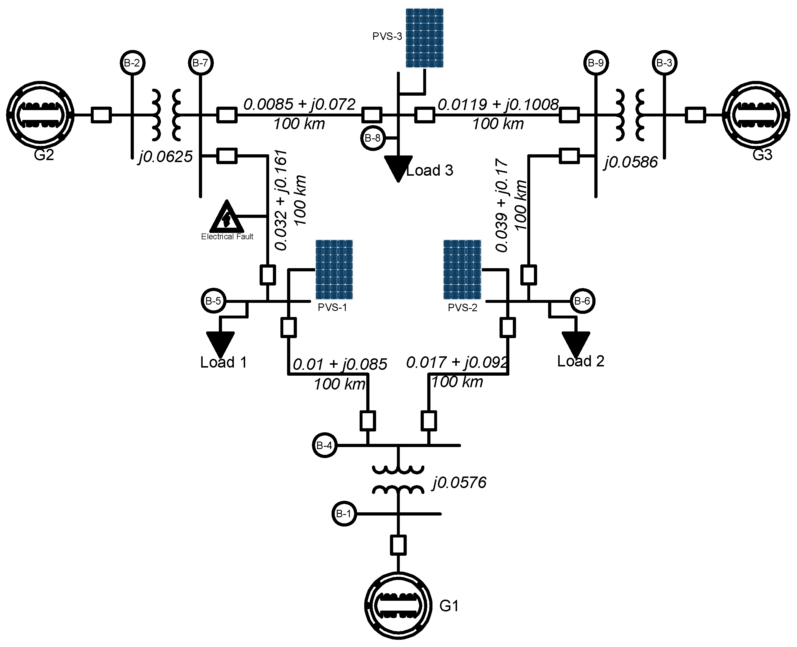
Figure 5.
Rotor angle displacement of the generators: (a) stable condition and (b) unstable condition.
Figure 5.
Rotor angle displacement of the generators: (a) stable condition and (b) unstable condition.
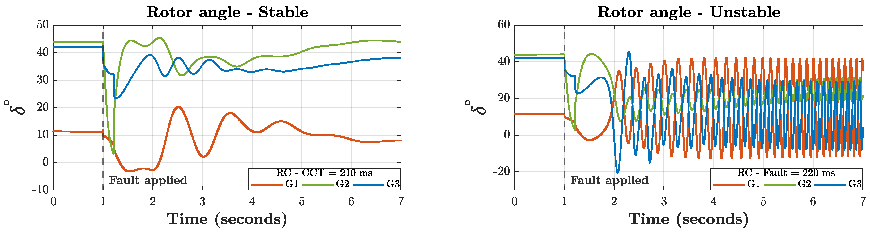
Figure 6.
Rotor angle displacement of the generators for 25% PV penetration: stable (left column) and unstable (right column) for concentrated and distributed injections.
Figure 6.
Rotor angle displacement of the generators for 25% PV penetration: stable (left column) and unstable (right column) for concentrated and distributed injections.
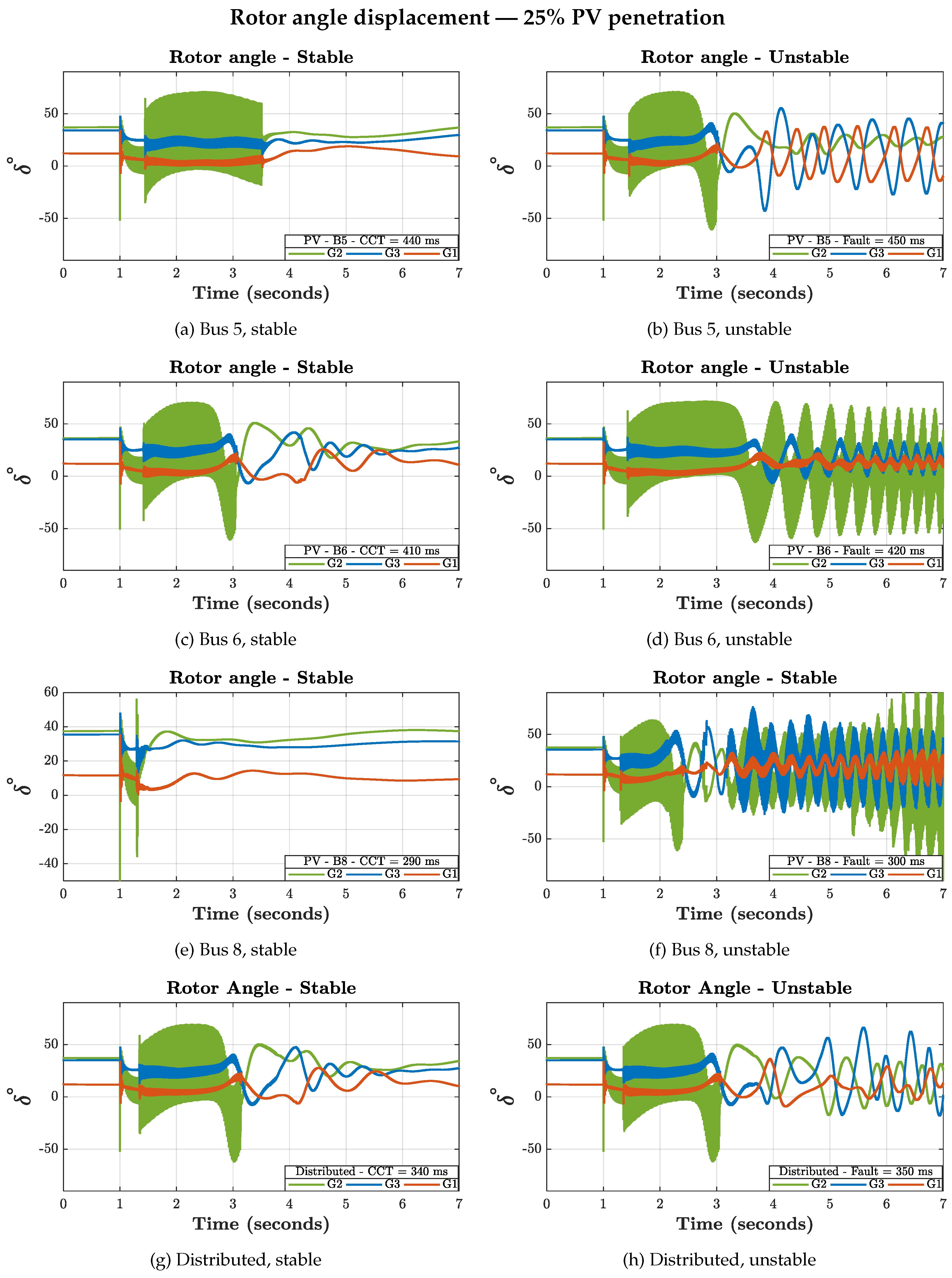
Figure 7.
Rotor angle displacement of the generators for 40% PV penetration: stable (left column) and unstable (right column) for concentrated and distributed injections.
Figure 7.
Rotor angle displacement of the generators for 40% PV penetration: stable (left column) and unstable (right column) for concentrated and distributed injections.
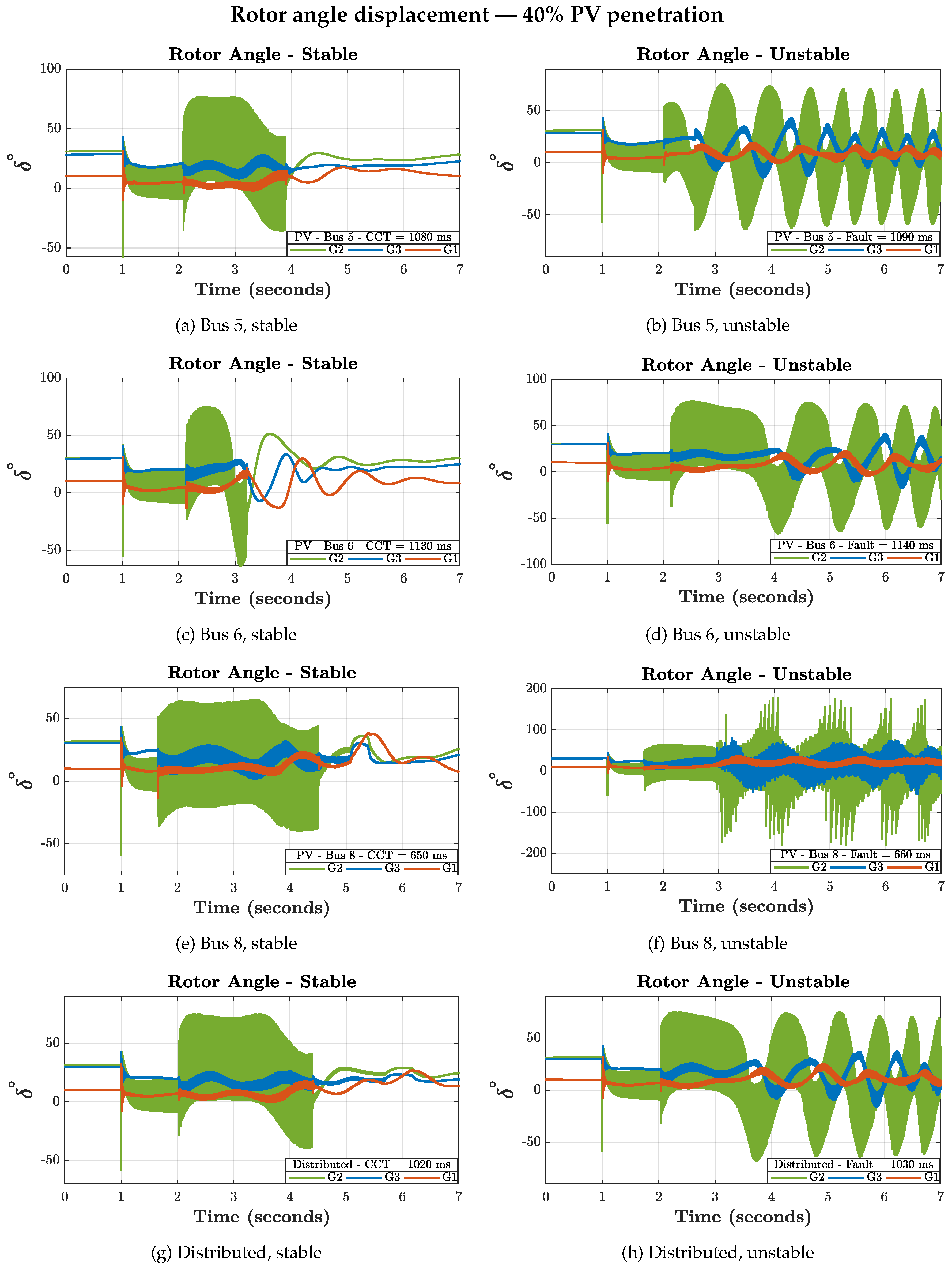
Figure 8.
Active power response of PV systems for concentrated injections under 25% and 40% penetration levels.
Figure 8.
Active power response of PV systems for concentrated injections under 25% and 40% penetration levels.
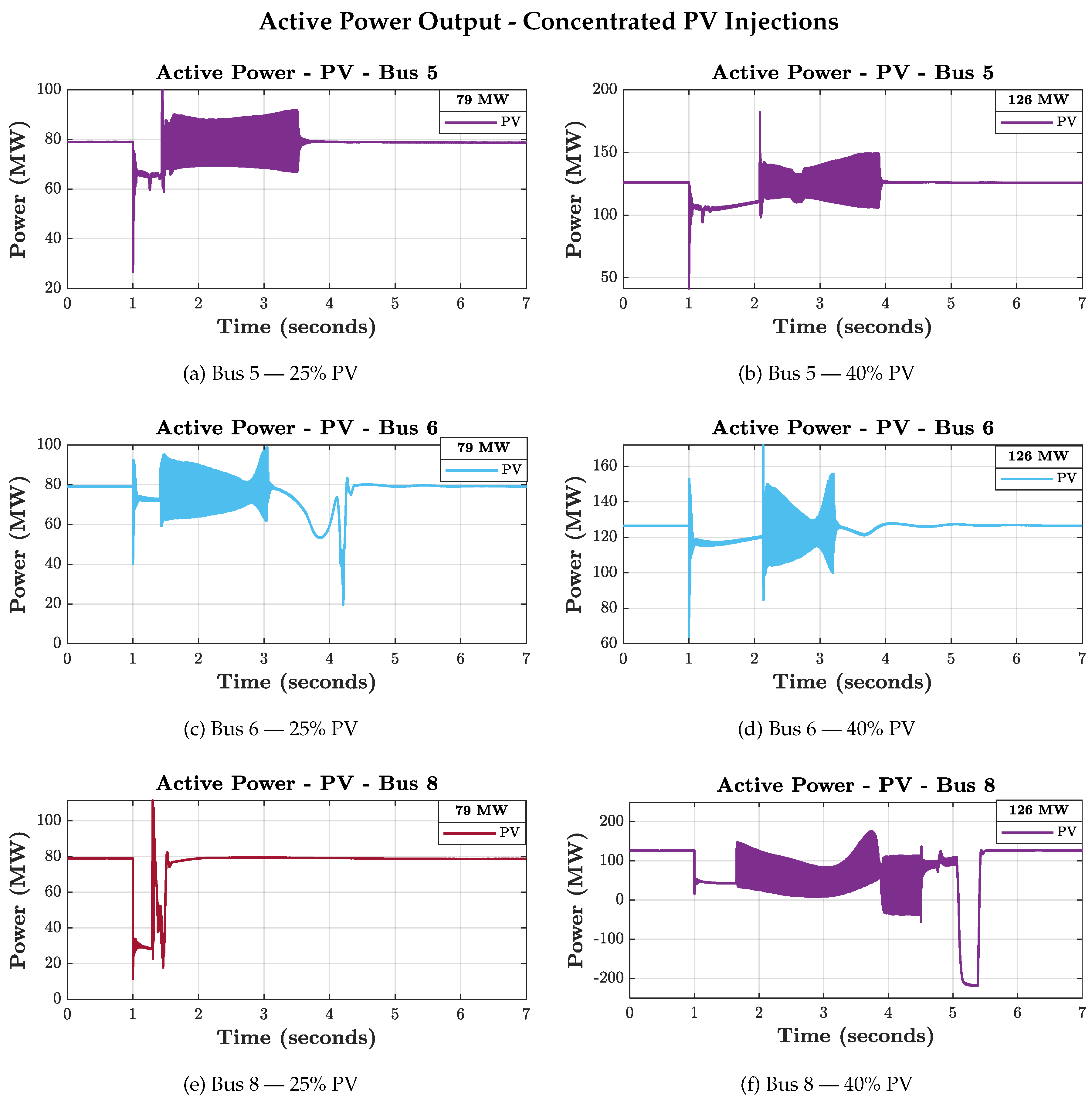
Figure 9.
Active power response of distributed PV systems for 25% and 40% penetration levels across buses 5, 6, and 8.
Figure 9.
Active power response of distributed PV systems for 25% and 40% penetration levels across buses 5, 6, and 8.
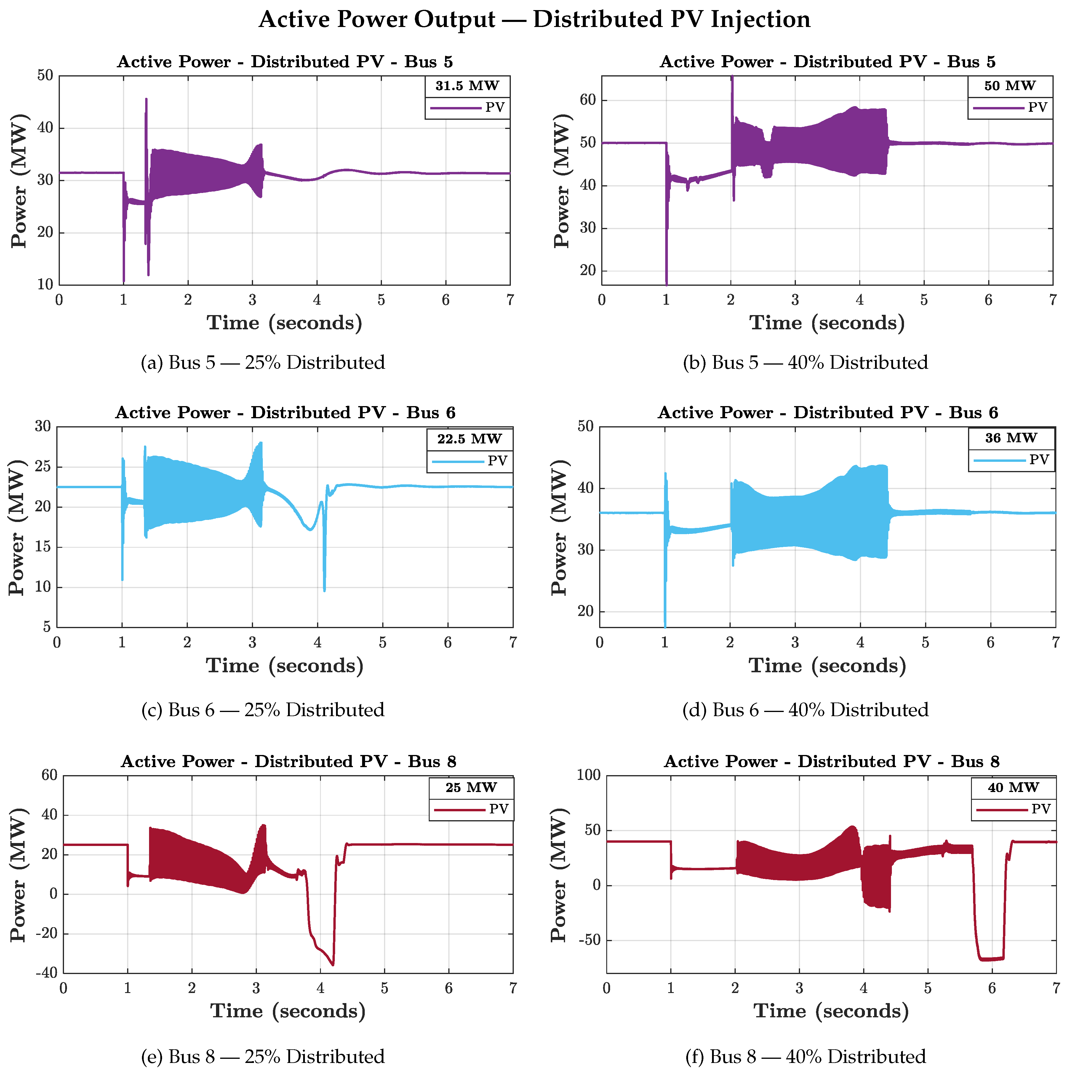

Table 1.
PV System Parameters.
| System Part | Components | Values |
|---|---|---|
| PV Array | Number of modules | 14700 |
| Modules per string | 7 | |
| Strings in parallel | 2100 | |
| PV Modules | Maximum power (W) | 414.801 |
| Open-circuit voltage (V) | 85.3 | |
| Voltage at MPP (V) | 72.9 | |
| Short-circuit current (A) | 6.09 | |
| Current at MPP (A) | 5.69 | |
| Cells per module | 128 | |
| DC-Link | Capacitor | 1.3021 F |
| Voltage | 240 V | |
| Filters | Resistor (R) | 156.06 m |
| Inductance (L) | 4.14 mH | |
| Transformer | Rated power | 6 MVA |
| Voltage ratio (kV) (AV/BV) | Yg 230 kV /260 V D1 | |
| (p.u.) | 0.0012 | |
| (p.u.) | 0.03 |
Table 2.
Bus Data of the IEEE 9-Bus Test System.
| Bus | Bus Type | V (p.u.) | (MW) | (MVAr) | (MW) | (MVAr) |
|---|---|---|---|---|---|---|
| 1 | Slack | 1.04 | – | 0 | 0 | 0 |
| 2 | PV | 1.025 | 163 | 0 | 0 | 0 |
| 3 | PV | 1.025 | 85 | 0 | 0 | 0 |
| 4 | PQ | 0 | 0 | 0 | 0 | 0 |
| 5 | PQ | 0 | 0 | 0 | 125 | 50 |
| 6 | PQ | 0 | 0 | 0 | 90 | 30 |
| 7 | PQ | 0 | 0 | 0 | 0 | 0 |
| 8 | PQ | 0 | 0 | 0 | 100 | 35 |
| 9 | PQ | 0 | 0 | 0 | 0 | 0 |
Table 3.
Dynamic Data of the Three Synchronous Generators Used in the IEEE 9-Bus System.
| Parameter | G1 | G2 | G3 |
|---|---|---|---|
| Type | Synchronous | Synchronous | Synchronous |
| Operation | Generator | Generator | Generator |
| Rated Power (MVA) | 512 | 270 | 125 |
| Nominal Voltage (kV) | 24 | 18 | 15.5 |
| Power Factor | 0.90 | 0.85 | 0.85 |
| H (s) | 2.6312 | 4.1296 | 4.768 |
| D (p.u./Hz) | 0 | 0 | 0 |
| (p.u.) | 0 | 0 | 0 |
| (p.u.) | 1.70 | 1.70 | 1.22 |
| (p.u.) | 1.65 | 1.62 | 1.16 |
| (p.u.) | 0.27 | 0.256 | 0.174 |
| (p.u.) | 0.47 | 0.245 | 0.25 |
| (p.u.) | 0.20 | 0.185 | 0.134 |
| (p.u.) | 0.20 | 0.185 | 0.134 |
| (p.u.) | 0.16 | 0.155 | 0.0078 |
| (s) | 3.80 | 4.80 | 8.97 |
| (s) | 0.48 | 0.50 | 0.50 |
| (s) | 0.01 | 0.01 | 0.033 |
| (s) | 0.0007 | 0.007 | 0.07 |
| (p.u.) | 0.09 | 0.125 | 0.1026 |
| (p.u.) | 0.40 | 0.45 | 0.432 |
Table 4.
Transmission Line Data of the IEEE 9-Bus System.
| Line No. | From Bus | To Bus | R (p.u.) | X (p.u.) | (p.u.) |
|---|---|---|---|---|---|
| 1 | 7 | 8 | 0.0085 | 0.072 | 0.0745 |
| 2 | 7 | 5 | 0.0320 | 0.161 | 0.1530 |
| 3 | 8 | 9 | 0.0119 | 0.1008 | 0.1045 |
| 4 | 5 | 4 | 0.0100 | 0.085 | 0.0880 |
| 5 | 6 | 4 | 0.0170 | 0.092 | 0.0790 |
| 6 | 9 | 6 | 0.0390 | 0.170 | 0.1790 |
| 7 (T1) | 1 | 4 | 0 | 0.0576 | 0 |
| 8 (T2) | 2 | 7 | 0 | 0.0625 | 0 |
| 9 (T3) | 3 | 9 | 0 | 0.0586 | 0 |
Table 5.
Simulation modes used for each scenario.
| Sources | Simulation Mode |
|---|---|
| Conventional generators | Phasor discrete mode; Sampling time: s; Solver: Ode1be. |
| Conventional generators and PV | EMT (Electromagnetic Transients); Discrete mode; Sampling time: s;Solver: ODE23tb (or Backward Euler for higher stability). |
Table 6.
Active PV and adjusted conventional generation power for each penetration level.
| Injection level | % | PV concentrated (MW) |
PV distributed (N5 / N6 / N8) (MW) |
G1 (MW) | G2 (MW) | G3 (MW) |
|---|---|---|---|---|---|---|
| Reference case | 0 | – | – | – | 163.0 | 85.0 |
| Moderate | 25 | 79.0 | 31.5 / 22.5 / 25.0 | – | 123.5 | 64.5 |
| High | 40 | 126.0 | 50.0 / 36.0 / 40.0 | – | 100.0 | 52.5 |
Table 7.
Critical Clearing Time for concentrated and distributed PV injections at penetration levels of 25% and 40%.
Table 7.
Critical Clearing Time for concentrated and distributed PV injections at penetration levels of 25% and 40%.
| Injection Scenario | CCT (25%) [ms] | CCT (40%) [ms] |
|---|---|---|
| PV at Bus 5 | 440 | 1080 |
| PV at Bus 6 | 410 | 1130 |
| PV at Bus 8 | 290 | 650 |
| Distributed (5/6/8) | 340 | 1020 |
Short Biography of Authors
 |
M. Jean Pierre graduated in Electromechanical Engineering in 2022 from the Faculty of Sciences at the State University of Haiti, with a thesis titled “Evaluation of the Thermal Performance of a Power Plant within the Metropolitan Power System and Proposal of Solutions to Improve its Energy Efficiency.” He is currently pursuing a master’s degree at the Instituto de Energías Renovables of the Universidad Nacional Autónoma de México (UNAM), where he conducts research on transient stability in power systems with high renewable energy penetration. |
 |
O. Rodríguez-Rivera holds a master’s degree in Energy Engineering from the Instituto de Energías Renovables at the Universidad Nacional Autónoma de México (UNAM) and a bachelor’s degree in Mechanical and Electrical Engineering from Tecnológico de Monterrey (ITESM). He has more than ten years of experience in the Mexican electrical sector, specializing in distribution grid design. He is currently pursuing a Ph.D. in Energy Engineering at IER–UNAM, focusing on microgrids and transient stability analysis. |
 |
E. Hernández-Mayoral received the M.Sc. and D.Sc. degrees in Electrical Engineering from the Technological Institute of Morelia in 2010 and 2015, respectively. He previously served as Professor and Researcher at Universidad del Istmo, Oaxaca, Mexico. He is currently a CONACyT Research Fellow at the Institute of Renewable Energies of the Universidad Nacional Autónoma de México (UNAM). His research interests include power quality, transient stability, and smart microgrids. |
 |
O. A. Jaramillo earned a B.Sc. in Mechanical-Electrical and Power Electronics Engineering from UNAM in 1996 (magna cum laude), receiving the “Ing. Joaquín Carrión Solana” medal. He also holds an M.Sc. in Solar Engineering (photothermal, magna cum laude, 1998) and a Ph.D. in Mechanical Engineering (magna cum laude, 2002), awarded the “Alfonso Caso” medal. He is a Level III National Researcher in Mexico’s National System of Researchers and has served on national committees for wind-turbine and solar-thermal technology development. Since 2003, he has been with UNAM’s Institute of Renewable Energy, working on solar-concentration systems, wind energy, and thermodynamic optimization. |
Disclaimer/Publisher’s Note: The statements, opinions and data contained in all publications are solely those of the individual author(s) and contributor(s) and not of MDPI and/or the editor(s). MDPI and/or the editor(s) disclaim responsibility for any injury to people or property resulting from any ideas, methods, instructions or products referred to in the content. |
© 2025 by the authors. Licensee MDPI, Basel, Switzerland. This article is an open access article distributed under the terms and conditions of the Creative Commons Attribution (CC BY) license (http://creativecommons.org/licenses/by/4.0/).
Copyright: This open access article is published under a Creative Commons CC BY 4.0 license, which permit the free download, distribution, and reuse, provided that the author and preprint are cited in any reuse.


