
Submitted:
10 December 2025
Posted:
11 December 2025
You are already at the latest version
Abstract
The position paper serves scientists from all scientific disciplines to get a quick, concise, and easy-to-understand primer that describes the basic principles of design and applications of massively-parallel computations and models. The thesis of the position paper is, “What is the estimated direction of development of massively-parallel computing techniques utilizing emergents as observed in all scientific disciplines?” The birth of massively-parallel computations (MPCs) in the 1940s is closely related to the development of both early computers and simulations of nuclear processes that are operating within matter. It would be demonstrated that MPCs are becoming front and center in many research areas after a long delay that was forced by the previous inaccessibility of MPC computers. Another impetus to the development of MPCs came in the form of generalization of mathematical descriptions of observed natural phenomena using differential equations. More specifically, discretization schemes of differential equations got implemented in MPC simulations. Those achievements opened doors to the development of advanced descriptions of natural phenomena. Currently, there exist a number of MPC techniques that are gaining an increasing influence on the description of self-organization, emergence, replication, self-replication, and error-resilience within living and nonliving systems. A promising class of cellular automata, which is capable of describing a wide range of processes observed within natural phenomena, is called emergent information processing (EIP). The EIP approach is opening doorstowards future descriptions of many observed biological phenomena that are notoriously resisting mathematical and computational descriptions. Fixed and ad hoc networks, which are observed in living and non-living systems, could be interpreted using EIP methodology; this offers an opportunity for computational studies of emergent processes operating within them. Demonstrated approaches represent a toolkit that could be applied in all areas of research that are dealing with living systems. The usefulness of the EIP approach is demonstrated on a special case of emergent synchronization simulation, which could be applied in the design of artificial, biocompatible pacemaker implants and computers utilizing emergent computations.
Keywords:
theory of computing
; complex systems
; emergence
; massively-parallel computing
; cellular automata
; emergent information processing
; error-resilience
; networks
1. Introduction
This review serves all scientists from all scientific disciplines to get a quick, concise, and easy-to-understand primer that describes the basic principles of design and applications of massively-parallel computations and models with a special focus on emergent computations. The entire methodology is based on cellular automata that represent the generic method of currently used massively-parallel computations.
| Thesis: What is the estimated direction of development of massively-parallel computing techniques utilizing emergents as observed in all scientific disciplines? |
The birth of massively-parallel computations (MPCs) is closely associated with the development of both early computers and descriptions of nuclear processes that are operating within matter and dates back to the 1940s; see Stanisław Ulam and John von Neumann [1,2,3,4]. Nuclear processes are inherently massively-parallel. Unfortunately, the reliability of components used in the computer design (e.g., ENIAC) and its predecessors [1,2] had been so low that it did not allow implementation of massively-parallel (MP) computers in the era of vacuum tubes. Hence, the so-called von Neumann design of computers utilizing the sequential topology was selected, where all the control unit, memory, arithmetic unit, and processor are separated, and they communicate using data-links; see Figure 1. MP implementations were left for a possible future hardware development. Later, the ideas seeded in this period of time led to the theoretical development of self-replicating cellular automata by von Neumann [2]. He was building upon the theoretical concepts developed during the 1940s while working on a novel theory of self-reproducing automata; this research was done without an implementation that was carried on later by others [4].
Later, what started as a teatime relaxation and playing with ideas had yielded John Conway’s massively-parallel cellular automaton called the ’Game of Life’ (GoL) [5] that was popularized in the journal Scientific American. The GoL, despite its inherent simplicity, displays endless complexity. Many generations of amateur and professional mathematicians are studying this ’toy model’ of living systems; they have grown their understanding of MPCs while using it.
A substantial increase in the computational power of processors in the 80s generated an important impulse for the development of MPCs, which was built on the mathematical descriptions of the observed natural phenomena using differential equations. It occurred that differential schemes of differential equations (known as numerical discretizations) could be easily implemented in N-dimensional cellular automata (because they lead to sparse matrices). Importantly, those implementations could be straightforwardly generalized (explained later on with an example) due to the high flexibility of the strictly localized definition of MP computing systems. In this way, interactions, which are impossible to implement in differential equations due to the averaging of their local values, are incorporated, which is a necessary step in the design of ordinary differential and partial differential equations, ODEs [23] and PDEs [24], respectively.
All the above-mentioned major contributions enabled the development of advanced descriptions of natural phenomena that are operating within complex systems. Currently, there exists a relatively wide range of computational techniques (see Table 1) that are gaining an influence on the description of self-organization, emergence, replication, self-replication, error-resilience, and other phenomena observed in natural processes. Those techniques can be, under certain circumstances, interpreted using fixed or ad hoc networks.
The performance of single computer processors met a physical bottleneck in the recent past. It naturally led to the development of multi-core processors and MP graphic cards. They require deeper understanding of deeply rooted principles of massive parallelism, as observed in natural phenomena.
The structure of the review is as follows: definition of cellular automata in Section 2, standard topology of CAs in Section 3, structure of discretization schemes in Section 4, topologies of networks in Section 5, link between CAs and networks in Section 6, emergent information processing (EIP) in Section 7, implementations and applications in Section 8, unpredictability of evolution of CSs in Section 9, EIP as prospective methodology in Section 10 (potential of EIP in linking unrelated research areas in Section 10.1), the big picture in Section 11, and sec:conclusions.
2. Definition of Cellular Automata
Before providing the cellular automata (CAs) definition, it is necessary to stress their important property: Turing machine equivalence [25]. In plain words, it means that cellular automata could compute everything that is computable [25]. Additionally, cellular automata serves as the prototype of all massively-parallel computations. The consequences of those facts are of the highest importance to all massively-parallel computing environments.
2.1. Standard Definition of Two-State Cellular Automaton
The formal definition of a two-state cellular automaton (CA) using squares in two dimensions follows; a generalization into N dimensions is straightforward [6,11]. Each cellular automaton is defined by the tuple where the symbol stands for a lattice, stands for a uniform neighborhood, stands for a micro-evolution rule, and stands for the global evolution.
The cellular space is defined by a lattice of cells in the following way
where the index i denotes the number of lines and reaches values , and the index j denotes the number of columns and reaches values . When the left and right edges and top and bottom edges get connected, periodic boundary conditions are created (the cellular space acquires the shape of a toroid).
By the definition, the state s of each cell can reach only two values
The von Neumann or Moore neighborhood N, which is composed of four or eight neighbors, respectively, is defined as follows
where defines the surrounding of each cell from which: (a) four nearest neighbors are selected (von Neumann neighborhood) or (b) eight nearest neighbors are selected (Moore neighborhood): . The central updated cell is always excluded from the neighborhood.
The change of the state of each single cell is defined by the evolution rule
which takes the state of the updated cell at the step t, along with states of all cells within the neighborhood as the input.
The evolution of the global state of the entire cellular automaton directly follows from the evolution of all cell
The standard definition of CA is typically focused on the micro-evolution rule, a.k.a., the transition rule whereas the set of possible shapes of the applied neighborhood is limited. Typically applied neighborhoods are the following: von Neumann (four first nearest neighbors) and Moore (eight first and second nearest neighbors together). Their variants have greater radii, e.g., for radius = 2, von Neumann has 12 neighbors [], and Moore has 24 neighbors []). Hence, the effects of changing neighborhoods remained under-explored until the development of the emergent information processing concept; see the next Section 2.2 and Section 7.
2.2. Definition of CAs with Changing Shape of Neighborhood: Under-Explored Class of CAs
Potentially, there are many existing possible neighborhoods for CAs under the assumption that the size of each neighborhood is substantially smaller than the size of the entire CA. The von Neumann and Moore neighborhoods are two of the most often used CA neighborhoods. The flexibility of the neighborhood definition in emergent information processing (EIP) approach—see Section 7 for the definition—enables a thorough exploration of neighborhood topologies and their effects on emergence.
Natural phenomena operating in nonliving and living systems are often relying on precisely defined topology of neighborhoods that are interconnecting matrix elements locally. Examples encompass not only the structure of crystals, chemical compounds, biochemical structures, DNA, the shape of proteins, brain structures, morphological growth, and structural components of living cells, but also many other structures not mentioned. The effects of various neighborhood topologies on the evolution of complex systems are still highly under-researched.
The only change in EIP—when compared to the standard cellular automaton definition—is within the pool of all possible neighborhoods of EIP, which is substantially enlarged. The total number of possible neighborhoods is . A generalized neighborhood N, where 8 neighbors are selected from 24 possible, is defined as follows
where defines the surrounding of each cell from which 8 neighbors are selected: .
The definition and details about the generalized neighborhood are available in Section 7 that is defining EIP.
3. Standard Topological Structures That Are Utilized in the Majority of Cellular Automata Models
There exist two major classes of natural phenomena when observed through the lenses of the regularity of their internal structure: lattice-like and non-uniform. An example of a lattice-like structure is solids with their physical lattices. Examples of non-uniform structure are water, living cells’ components, proteins, cellular building blocks, tissues, societies, gasses and glasses.
| Each lattice-based cellular automaton can be rewired into a uniform graph. It is made by connecting the center of each cell to the centers of its neighbors. |
The lattice shapes that are commonly used in cellular automata—square, hexagonal, and triangular (see Figure 2)—could be rewired into uniformly shaped graphs. For example, a square lattice of cells, which is shaped into a uniform graph, is shown in Figure 3 (A). Such graphs, while subjected to the simple micro-evolution of nodal values, utilize the uniform evolution rule and neighborhood.
4. Numerical Discretizations of Differential Equations Explained on Simple Example
The idea that links ODEs and PDEs together with CA dates back to the seminal work of Toffoli, where CAs are presented as an alternative [7] to differential equations. There are presented ideas about simulating physics using CAs provided by Vichniac [8] in the same journal volume. Numerical discretization schemes of ODEs and PDEs are provided in detail within the book of Marchuk [26]. In the following is demonstrated an example of the procedure that takes a discretization scheme of one physical problem and transforms it into a CA transition rule—which is also known under the names “the evolution rule” and “evolution function”.
As an example, the differential equation, which is representing heat transfer in one dimension (e.g., a narrow wire), is demonstrated; it has the following form
where D is the diffusion coefficient, and f and g are given functions. The boundary conditions are omitted for simplicity. The equation is defined for the region where and .
The derivation of an explicit finite difference scheme of the one-dimensional heat equation follows; see the book for details and other discretization schemes [26]. The idea of the finite differences method is to replace time and spatial derivatives by approximations.
The discretization scheme of the first time derivation gives
where the temporal difference will be replaced by the symbol , it gives . The index k is used for spatial discretization, and the index j is used for temporal discretization.
The discretization scheme of the first spatial derivation gives
where the spatial difference is replaced by the symbol h; it gives .
The discretization scheme of the second spatial derivation using the explicit scheme yields
The final discretization scheme, when both temporal and second spatial discretizations are put together, yields
what is called the explicit discretization scheme (implicit and mixed are the other two possible discretizations).
CA implementation could be easily derived from the explicit scheme
The Equation (4) is inserted into the evolution rule, see Equation (4), which is valid for every cell of the given CA except for the boundary conditions that are not presented here; see Figure 4 for a schematic depiction of the actions of the evolution rule. Details are presented in the book of Marchuk [26].
The interpretation of the relationship between CAs and discretization schemes of differential equations motivated the development of the MP model of dynamic recrystallization [27,28]. During the development of the DRX model, many different evolution rules were tested; this knowledge constituted the basic knowledge about evolution rules that later enabled studies of more complicated natural phenomena observed within complex systems; see [11,13,29].
Massive parallelism is critical in the design of many models of natural phenomena observed within complex systems. Without utilization of the MP approach, models of natural phenomena that are observed in complex systems fail in the majority of cases; see, e.g., unsuccessful DRX models based on Monte Carlo simulations vs. successful MP models [27,28].
5. Topology of Various, Generic Types of Non-Uniform Networks That Are Observed Within Natural Systems
Various generic types of networks—see Table 2 and Figure 5 for their detailed description—serve as a scaffold to a wide spectrum of micro-evolution processes that are operating above them. Both networks and processes work in synergy. Together, they generate emergent structures that are observed across the entire spectrum of scientific disciplines. It would be important to study those graphs systematically, which is beyond the scope of this review; see the seminal works in [30,31] for details. Nevertheless, examples provided in Table 2 and Figure 5 give a good starting point to everyone who needs to go beyond the cellular automata methodology of description of complex systems.
Micro-evolution rules that operate above various types of networks are worth studying. Cellular automata are typically designed above uniform (regular) networks. It is worth mentioning that some CAs are being designed above non-uniform networks such as random, small-world, and scale-free.
The advantage of CAs, which are defined above uniform networks, is their uniformity of neighborhood and micro-evolution rule. CAs that are operating above non-uniform networks do not provide such luxury; in such cases, both neighborhood and micro-evolution rule must accommodate the change of the number of links from one node to another node! An important note: neural networks utilize the directed processing of information, whereas CAs do not! CAs provide more freedom in computations.
6. Links Between Cellular Automata and Networks
The underlying lattice of uniform CAs—where the lattice represents one of the major parts of the definition of each CA at its constituting level (see Section 2)—could be interpreted as a perfectly uniform graph where each vertex is connected to the identical number of its closest neighbors; see Figure 2 for examples. Contrary to those common cases of CAs that have uniform graphs, there exist CAs that could be represented by non-uniform graphs; see examples shown in Figure 3 and Figure 5. Various naturally observed examples of non-uniform graphs were provided in Section 5; see Table 2 and Figure 5.
| Link Between CAs and Graphs: Surprisingly, topologically simple, uniform graphs can perform fairly complicated Turing machine equivalent computation using simple micro-evolution rules! It was proven for cellular automata [25] in the 70s. |
A detailed overview of non-uniform graphs is beyond the scope of this review; details and more examples could be found in [30,31]. Another huge class of CA descendants is overviewed in the book about the principles of agent based modeling [9], which describes a generalization of cellular automata with mobile ’lattice’ elements that are called agents; in this case, the ’lattice’ is dynamically changing its shape in time; see Figure 6.
This brings us to the major theme of the following sections: graph properties of the lattice, along with the topology of the applied neighborhood, have a huge impact on the overall behavior of the entire system. It was found that mere changes of the neighborhood topology generate an unexpectedly profound effect on the systemic outcome. Surprisingly, it is possible to define robust systems performing various tasks just by applying a specific configuration of the neighborhood’s topology.
7. Emergent Information Processing (EIP)
7.1. Definition of EIP
A very brief definition of EIP follows; a detailed definition is provided in [11,12]. The EIP method is the generalization of the well-known cellular automaton called the ’Game of Life’ (GoL) [5] that was developed by J.H. Conway. EIP CA is the same as the GoL CA except for the neighborhood; see Section 2.1 for details. The neighborhood of the GoL CA is fixed to eight nearest neighbors. On the contrary, the neighborhood of EIP CA uses a selection of eight neighbors from 24 possible (), which are pre-selected from the extended neighboring region of the updated cell. Such a neighborhood remains identical for all updated cells during the entire simulation.
7.2. Some Examples of EIP
Among many observations that were achieved during the study of EIP models using software GoL-N24 [32], several are standing out. An important behavior is generated by the rule #459744 and its three symmetrical variants [11]; it expresses a spontaneous creation of a two-level emergent system that emerges from random initial conditions. There are observed spontaneously emerging breading-ships of the first-level that bread ships of the second-level; see Figure 7. The original GoL simulations of logic gates OR and AND are provided in Figure 8.
7.3. Video-Database of EIP
To enable an easy orientation in observations and all results that have been found in many EIP models, which are based on many different neighborhoods, a systematic video-database of links to important animations of simulations is available [29].
7.4. EIP Software
An open-source Python software that is simulating EIP is available under the name GoL-N24 [32]. Everyone could use it to design their own neighborhoods and run their simulations. A simpler version of GoL [33], which has a total length of under 100 lines, enables one to understand the basic principles of CA design. Emergent information processing and design of the GoL-N24 software are described in the article [11] in detail.
8. Implementations and Applications
Theory is always best understood through its applications. This is the main goal of this section. The application of EIP to error-resilient S2D-SP [13] is opening a novel area of research of emergent modeling in biology; for details, see the following Section 8.4.
8.1. Hardware Implementations of CAs
The first hardware implementation of CAs had been developed by Toffoli [34] in the early 80s. This implementation enabled the study of large CA models prior to the occurrence of fast personal computers. Over the years, many other hardware implementations were developed; see a selected list of them in Table 3. For example, one of the latest implementations is optoelectronic computing devices that are based on multiplexing impulses of a femtosecond laser [35]. Other optoelectronic approaches are currently being developed.
8.2. Software Implementations of CAs
Over the past fifty years many software implementations of CAs were developed using various software languages: C, C++, Python, and Logo; see Table 4 for a list of currently used CA software implementations.
Both hardware and software CA implementations have been crucial in achieving a deeper understanding of MPCs. It is impossible to experiment on the majority of complex systems. Therefore, the only way to gain their deeper understanding is to simulate them.
8.3. Biological Applications
Current biological studies of morphological development and regeneration, which are carried out on flatworms [52] and salamanders, confirm the hypothesis that morphological structures are of the emergent nature. It had been demonstrated by a number of experiments—which manipulated the standard morphology of species by mere adjustment of cell membrane potentials—that such a possibility exists beyond any doubt [53,54,55,56].
Collective intelligence of evolution and development is becoming increasingly studied [57]; it opens new vistas in MP systems research. One of the very important outcomes is breast cancer treatment using light-gated ion translocators to control tumorigenesis [58,59].
Ad hoc networking of brain structures in solving different tasks: The same structures are involved in the processing of different tasks. The structure is the same, but tasks differ; e.g., see multi-level clustering of dynamic directional brain network patterns [60]. To summarize research on biological systems, the following application of EIP is addressed.
8.4. Generic Template of Artificial, Bio-Compatible Pacemaker Replacement
In 2009, an emergent system [13] called the semi-two-dimensional synchronization problem (S2D-SP) had been accidentally discovered. S2D-SP itself is based on a specific neighborhood within the EIP computing system that automatically generates emergent synchronization in a CA; see Figure 9. It is discussed in [13] that this generic template of the synchronization problem could serve as the starting point of the development of an implantable, biocompatible, tissue-engineered pacemaker replacement. Additionally, it could serve as a prototype in the development of novel directions within the domain of emergent computing (part of unconventional computing).
In computer science, there exists the generic problem, which is called the firing squad synchronization problem (FSSP) [61,62,63,64,65], that represents a widely studied problem of synchronization within MP systems. Another widely studied generic MP problem is the density classification task (DCT) [66,67,68,69]. The emergent system [13], called S2D-SP, is very close to the original FSSP; see details in [13] .
8.5. Unconventional Computing
Observed functioning of biological tissues, organs, structures, and body systems reveals the existence of dynamic stability not only in, e.g., the heart tissues [13], but, also, in brain centers during the solution of various tasks and reaching goals [60]. Those observations point towards the existence of emergent computing in biological systems that could reuse the identical substrate for different computational tasks. Research confirms that the hijacking of artificial NNs [70,71,72,73,74], which are trained for one task, to perform another task with surprisingly high efficiency is consistent with biological observations [70].
| Has science arrived at a novel understanding of biology? Research carried on the morphological development of animals points towards the understanding that genes define building blocks. The structural design of morphology is defined by emergent processes. |
Research carried out on the morphological development of flatworms and axolotls [52,53,54,55,57,59] generates valuable insights into emergent ’computations.’ Additionally, morphology reaches various goals within the MP living substrate, where each living cell serves as the constitutional unit of the dynamically changing, ad hoc matrix (network).
Global solutions—which are called morphological structures in biology—emerge due to intercellular communication, mutual negotiation, and long-range consensus without the existence of any global coordinator.
Mathematical descriptions of EIP [11,12,13]—which are based on the used software implementations: the simplest GoL [33], r-GoL [45], and GoL-N24 [32]—provide a useful toolkit that enables everyone to explore emergence not only in biology. Another prospective area of applications is emergent computing and problem solving. The goal is to develop a universal computing medium that will allow us to solve a wide range of MP tasks utilizing self-organization and emergence.
| The term “unconventional computing” is unconventional from the human perspective in the context of the current scientific understanding and technological development. Unconventional computing [75] is very conventional in many of the by-scientists-observed natural and biological phenomena. We must make this point very clear. |
9. Irreducibility and Unpredictability of Complex Systems Evolution
Cellular automata represent a generic prototype of all MPC systems, according to many researchers working within complex systems. Despite the apparent simplicity of CAs’ definition, their behavior cannot be predicted in the majority of sufficiently complicated settings. It has been known for a long time that the evolution of a sufficiently complicated cellular automaton cannot be analytically predicted [25]. The only way to know the evolution of CAs is to simulate them or observe their real-life equivalent.
It had been demonstrated that the GoL CA is universal [76,77,78,79,80]. In other words, the GoL CA is Turing equivalent [25], which means that GoL can compute everything computable in the same way as the Turing machine does. One example of universality is the existence of logic gates that are implemented in the GoL; see Figure 8 for examples of AND and OR logic gates.
Irreducibility of CAs, as discussed above, points towards and clearly demonstrates a huge obstacle in theoretical studies of complex systems and development of their reliable models.
| Irreducibility of CAs: In general, there is no way to predict future states of an operating MP system using current knowledge of complex systems and their simulations except in some special cases. |
Unexpectedly, it had been found that complex systems have one property that makes their use and applicability challenging due to security reasons. It was found and demonstrated in research on hijacking of neuronal networks [70,71] that there exists a possibility to misuse trained neuronal networks (NN) for other computations. Hijacking of NNs is producing surprisingly good results.
| The Ultimate Goal: Is it possible that one universal ’computing’ structure could be utilized in different ’computing’ scenarios? |
The hijackability of complex systems has far-reaching consequences, not only in computational security, but also in opening new vistas of biological research. There exists a chance that all biological systems utilize some specific approach of structural design, which permits flexible ’computing,’ and that allows adjustment of this ’computing’ machinery to the actual needs. In other words, one ’computing’ structure, which is solving one task, could be applied to multitude of different tasks.
10. Prospective Methodology of Solving Scientific Problems
In this section, perspective directions of the future EIP development are briefly overviewed. A general understanding of EIP within the framework of the meta-level of scientific descriptions is described in detail in [11,12,13]. Animations of EIP are always carrying very dense information that could be easily compared to real, observed natural phenomena; for examples, see Figure 7, Figure 8 and Figure 9. An entire PDF file [29] contains links to many EIP animations and provides a concise, visual introduction into the subject!
10.1. EIP Has Potential to Bridge Uncharted Areas Within Contemporary Research
EIP represents an unconventional attempt to formulate a way that has the potential to describe a wide range of observed phenomena across the entire spectrum of scientific disciplines—physics [7,8,27,28], quantum mechanics (QM) [81], chemistry, biochemistry, biology [52,53,54,55,57,59], medicine[13,56,58,82], AI [12], theory of computing [13,18], and complex systems themselves. Many observed phenomena resist their theoretical and computational description while using standard mathematical and computational approaches.
| Paradigm Shift: Is it the right moment to reframe our understanding of the mathematical description of nature and the phenomena observed within it? |
As already stated in the previous section, nature has found a surprisingly efficient means of problem solving, which is also known under the term ’computing.’ This ’computing’ operates within biological systems and, probably, even in a simplified form within physical systems. Is it possible to decipher this type of ’computing?’
EIP research suggests [11,12,13] a possibility of the existence of a unified matrix along with a set of micro-evolution rules, which together are called the constituting level of an MP system. When a selected constituting level of an MP system, which is chosen from many possible configurations, receives inputs, it generate activity. An evolving MP system generates phenomena. Some of the MP systems spontaneously generates emergents. This leads to the example demonstrated in Section 10.3.
10.2. Motivations of EIP definition
During PhD studies, the author of this position paper had been developing a computational description of dynamic recrystallization, which operates in metals during high deformation rates and elevated temperatures, that requires the application of MPC methodology [27,28]. Gradual development of the CA model led to the exploration of many different local evolution rules that revealed an unparalleled flexibility of MP descriptions of natural phenomena in comparison with ODE- and PDE-based descriptions.
Surprisingly, during this period of time, quite a few already known local rules—e.g., the one that led to the snowflake-like fractal—had been rediscovered. The concept of EIP became even clearer after studying self-organization, the firing squad problem (synchronization) [13], and the density classification problem (unpublished). Those experiences led to the development of EIP twenty years later.
10.3. Template of Synchronization Problem
Figure 9 depicts snapshots from the synchronization problem S2D-SP (link to animations in [13]). The simple solution of S2D-SP, which is faster than the width of the used lattice of cells, represents an excellent example of emergent computation capabilities. The S2D-SP utilizes a specific, extended neighborhood.
In addition to S2D-SP’s simplicity, the given solution is robust against injections of a small fraction of errors into the simulation. Hence, emergence is partially error-resilient in this particular case, which is even more important than the speed of the simulation!
11. The Big Picture: Putting EIP Computing into Broad Context
To put the described concept of EIP into a broad context, the meta-level of computing is briefly reviewed in this section. It enables readers from different research areas to find relevant computational concepts for a specific observed phenomenon.
11.1. Overview of Known Computing Methods
During several past decades, many studies of unconventional computing—which is observed across a wide range of natural systems, including phenomena that operate there—were conducted; e.g., see [22,75,83,84].
A wide range of computational methodologies—which are based on various natural phenomena—have been developed; see Table 5 for a list of the most important methods, including many citations.
11.2. Is There Existing Universal Computing Topology in Each Given Massively-Parallel Computational System?
From experiments performed on ANNs, it becomes evident that they could be hijacked [70,71,72,73,74]; see Section 8.5. Originally, all those ANNs had been trained to perform one specific task. Yet, when the input data are sufficiently distorted, the trained ANNs are capable of performing another task with quite high performance.
| Universal Computing Substrate: The question is whether there exists a possibility of the existence of a universal computing substrate in MPCs. In other words, could each MPC system implicitly contain configurations that are computationally universal? |
There exists a surprising consequence to all MPC systems besides, security concerns, which are important for huge data centers running AI software and the safety of devices using AI. A non-negligible chance exists that each MP system contains at least one configuration that is capable of universal computation, as was already proven for GoL CA [25]. This observation is opening new vistas in biological research and consequently in the design of artificial computing environments.
11.3. Noumenal and Phenomenal Realms
“’Noumenon’—from the Greek word —is knowledge and is assumed to be an object that is independent of human senses; it is a thing-in-itself or something that is thought. In other words, noumenal means real. The term “noumenon” is used as the opposite of “phenomenon,” which refers to an object perceived by the senses [94].”
Science, since its birth, has been facing the problem of whether phenomena are primary or whether there exists something more, something deeper. Plato’s allegory of chained observers in a cave who are observing the shadows of reality is a very well-known description that has existed for millennia.
When we return to EIP, there exists a possible meta-level point of viewing it. Noumenal could be defined by the matrix and micro-processes, while phenomenal would be, in such a case, all self-organizing, self-assembling, and emerging simulated structures; see details in Table 6.
Conclusions
The main goal of this position paper is to provide an introduction into emergent computing within the historical context. Numerical experiments—which are utilizing MPCs, CAs, and ABMs, along with novel insights into the functioning of biological systems—have a strong impact on the current understanding of emergent computation.
Despite the lack of a unifying theory, knowledge achieved in EIP points in a certain direction where we anticipate substantial breakthroughs in the near future. Everyone who wants to reach the frontiers of the current research in the emergent computing quickly will find this text helpful.
Two major groups of researchers would benefit from the knowledge covered in this text: biologists and computer designers. Biologists will better understand the self-organizing and emergent properties of living systems at all of their scales. Computer designers and computer scientists would benefit from a deeper understanding of the principles of emergent computing, which will translate into a higher robustness of computing.
Funding
This research received no external funding.
Data Availability Statement
Python software GoL-N24 is available at [32]. Animations of S2D-SP are available at the web-page https://researchgate.net/publication/388224794.
Acknowledgments
This publication is entirely dedicated to the people of the Czech Republic, and is entirely the result of independent research that was fully sponsored by the author himself without any kind of external support.
Conflicts of Interest
The author declare no conflicts of interest.
Abbreviations
The following abbreviations are used in this manuscript:
| CS | complex system |
| MP | massively-parallel |
| MPC | massively-parallel computing |
| CA | cellular automaton |
| EIP | emergent information processing |
| GoL | ’Game of Life’ |
| r-GoL | resilient GoL |
| GoL-N24 | GoL having extended neighborhood |
| S2D-SP | semi-2D synchronization problem |
| FSSP | firing squad synchronization problem |
| DCT | density classification task |
| NN | neural network |
| ANN | artificial neural network |
| ODE | ordinary differential equation |
| PDE | partial differential equation |
| ABM | agent-based model |
References
- Ulam, S.; von Neumann, J. Concept of Cellular Automata Invented in Los Alamos Laboratory. proposal to von Neumann.
- von Neumann, J. Theory of Self-Reproducing Cellular Automata, 1 ed.; University of Illinois Press: Urbana and London, 1966; p. 388.
- Ulam, S. Random Process and Transformation. In Proceedings of the Proceedings of the International Congress of Mathematicians, Cambridge, MA, USA, 30 August – 6 September 1950; Vol. 2, pp. 264–275.
- Pesavento, U. An implementation of von Neumann’s self-reproducing machine. Artificial Life 0194, 2, 337–354. [CrossRef]
- Gardner, M. The fantastic combinations of John Conway’s new solitaire game "life". Scientific American 1970, 223, 120–123. https://www.scientificamerican.com/article/mathematical-games-1970-10.
- Illachiski, A. Cellular Automata: Discrete Universe; World Scientific Publishing Company, 2001; p. 840.
- Toffoli, T. Cellular automata as an aternative to (rather than an approximation of) differential equations in modelling physics. Physica D: Nonlinear Phenomena 1984, 10, 117–127. [CrossRef]
- Vichniac, G. Simulating physics with cellular automata. Physica D: Nonlinear Phenomena 1984, 10, 96–116. [CrossRef]
- Illachiski, A. Artificial War: Multiagent-based Simulation of Combat; World Scientific Publishing Company, 2004; p. 747.
- Sukop, M.; Thorne, D., Lattice Gas Models. In Lattice Boltzmann Modeling: An Introduction for Geoscientists and Engineers; Springer: Berlin, Heidelberg, 2006; pp. 13–26. [CrossRef]
- Kroc, J. Emergent Information Processing: Observations, Experiments, and Future Directions. Software 2024, 3, 81–106. [CrossRef]
- Kroc, J. Complex Systems with Artificial Intelligence – Sustainability and Self-Constitution. In Difference between AI and Biological Intelligence Observed through Lenses of Emergent Information Processing; Lopé-Ruiz, R., Ed.; IntechOpen: Rijeka, 2024. [CrossRef]
- Kroc, J. Biological Applications of Emergent Information Processing: Fast, Long-Range Synchronization. [CrossRef]
- Fish, J.; Wagner, G.; Keten, S. Mesoscopic and multiscale modelling in materials. Nature Materials 2021, 20, 774–786. [CrossRef]
- Agarwal, M.; Pasupathy, P.; Wu, X.; Recchia, S.; Pelegri, A. Multiscale Computational and Artificial Intelligence Models of Linear and Nonlinear Composites: A Review. Small Science 2024, 4, 2300185. [CrossRef]
- Samek, W.; Montavon, G.; Lapushkin, S.; Anders, C.; Müller, K.R. Explaining Deep Neural Networks and Beyond: A Review of Methods and Applications. In Proceedings of the Proceedings of the IEEE, 2021, Vol. 109, pp. 247–278. [CrossRef]
- Miyenye, I.; Swart, T. A Comprehensive Review of Deep Learning: Architectures, Recent Advances, and Applications. Information 2024, 15, 755. [CrossRef]
- Barbosa, V. Massively Parallel Models of Computation: Distributed parallel Processing in Artificial Intelligence and Optimization; Ellis Horwood: USA, 1993; p. 250. [CrossRef]
- Cook, M.; Rothemund, P.; Winfree, E. Self-Assembled Circuit Patterns. In Proceedings of the DNA Computing: DNA 2003; Chen, J.; Reif, J., Eds., Berling/Heidelberg: Germany, 2004; pp. 91–107. [CrossRef]
- Yang, S.; Bögels, B.; Wang, F.; Xu, C.; Dou.; H. Mann, S. Fan, C.; de Greef, T. DNA as a universtal chemical substrate for computing and data storage. Nature Reviews Chemistry 2024, 8, 179–194. [CrossRef]
- Carignano, A.; Chen, D.; Mallory, C.; Wright, R.; Klavins, E. Modular, robust, and extendible mullticellular circuit design in yeast. eLife 2022, 11, e74540. [CrossRef]
- Adamatzky, A. A brief history of liquid computers. Philosophical Transactions of the Royal Society B 2019, 374. [CrossRef]
- Arnold, V. Ordinary Differential Equations, 1 ed.; Universitext, Springer: Berlin, Heidelberg, 1992; p. 338.
- Evans, L.C. Partial Differential Equations: Second Edition; Vol. 19, Graduate Studies in Mathematics, Department of Mathematics, University of California, Berkeley, American Mathematical Society, 2010; p. 749.
- Wainwright, R. Life is Universal! In Proceedings of the WSC’74: Proceeddings of the 7th Conference on Winter Simulations, January 14–16, 1974, 1974, Vol. 2. [CrossRef]
- Marchuk, G.I. Methods of Numeriacal Mathematics, 2 ed.; Stochastic Modelling and Applied Probability, Springer: New York, NY, 1982.
- Kroc, J. Simulations of Dynamic Recrystallization by Cellular Automata. PhD thesis, Charles University, Prague, The Czech Republic, Ovocný trh 11, 2001. http://www.researchgate.net/publication/311733496.
- Kroc, J. Application of Cellular Automata Simulations to Modeling of Dynamic Recrystallization. In Proceedings of the Int. Conf. Amsterdam. Springer, 2002, Vol. 2329, Lecture Notes in Computer Science, pp. 773–782. http://www.researchgate.net/publication/225670793.
- Kroc, J. Exploring Emergence: Video-Database of Emergents Found in Advanced Cellular Automaton ’Game of Life’ Using GoL-N24 Software. www.researchgate.net/publication/373806519, Complex Systems Research, Pilsen, The Czech Republic, 2024.
- Réka, A.; Barabasi, A.L. Statistical mechanics of complex networks. Reviews of Modern Physics 2002, 74. [CrossRef]
- Barabasi, A.L. Linked: How Everything is Connected to Everything Else and what it Means for Business, Science, and Everyday Life; Basic Books, 2014.
- Kroc, J. Exploring Emergence: Python Program GoL-N24 Simulating the ’Game of Life’ Using 8 neighbors from 24 Possible, 2022. https://www.researchgate.net/profile/Jiri-Kroc/365477118.
- Kroc, J. Python software simulating simplest GoL, 2021. https://www.researchgate.net/profile/Jiri-Kroc/355043921.
- Toffoli, T.; Margolus, N. Cellular Automata Machines: A New Environment for Modeling; Scientific Computing and Engineering, The MIT Press, 1987.
- Li, H.Y.; Leefmans, C.R.; Williams, J.; Marandi, A. Photonic elementary cellular automata for simulation of complex phenomena. Light: Science & Applications 2023, 12. [CrossRef]
- Cagiggas-Muñiz, D.; Diaz-del Rio, F.; López-Torres, M.; Jiménez-Morales, F.; Guisado, J. Developing Efficent Discrete Simulations on Multicore and GPU Architectures. Electronics 2020, 9, 189. [CrossRef]
- Morán, A.; Frasser, C.; Roca, M.; Rosselo, J. Energy Efficient Pattern Recognition Hardware with Elementary Cellula Automata. IEEE Transactions on Computers 2019, 69. [CrossRef]
- Wang, H.; Wang, J.; Yan, S.e.a. Elementary cellular automata realized by stateful three-memristors logic operations. Scientific Reports 2024, 14, 2677. [CrossRef]
- Treml, L.; Bartocci, E.; Gizzi, A. Modeling and Analysis of Cardiac Hybrid Cellular Automata via GPU-Accelerated Monte Carlo Simulation. Mathematics 2020, 9, 164. [CrossRef]
- Halbach, M.; Hoffmann, R. Implementing Cellular Automata in FPGA Logic. In Proceedings of the 18th Int. Parallel and Distributed Processing Symposium (IPDPS), Santa Fe, New Mexico, USA, 2004. [CrossRef]
- Bakhteri, R.; Cheng, J.; Semmelback, A. Design and Implementations of Cellular Automata on FPGA Hardware Acceleration. Procedia Computer Science 2020, 171, 1999–2007. [CrossRef]
- Dascalu, M. Cellular Automata Hardware Implementations–an Overview. Romanian J. of Information Sci. and Techn. 2016, 19, 360–368.
- Charbouillot, S.; Perez, A.; Fronte, D. A Programmable Hardware Cellular Automaton: Example of Data Flow. VLSI Design 2008, 1. [CrossRef]
- Sirakoulis, G., Cellular Automata Hardware Implementation. In Cellular Automata: A Volume in Encyclopedia of Complexity and Systems Science, Second Edition (Encyclopedia of Complexity and Systems Science Series); Springer US: New York, NY, 2018; pp. 555–582. [CrossRef]
- Kroc, J. Python program simulating cellular automaton rGoL that represents robust generalization of ’Game of Life’, 2022. https://www.researchgate.net/profile/Jiri-Kroc/358445347.
- Rucker, R.; Walker, J. CA simulator CelLab use WebCA engine to run rules designed in JavaScrip and Java, 1989-continues. https://www.fourmilab.ch/cellab.
- Trevorrow, A.; Rokicki, T.e.a. Golly: open-source, cross-platform application for exploring cellular automata, 2024. https://www.golly.sourceforge.io.
- Kopfler, E.; Scheintaub, H.; Huang, W.; Wendel, D., StarLogo TNG: Making Agent-Based Modeling Accesible and Appealing to Novices. In Artificial Life Models in Software; Springer: London, 2009; pp. 151–182. [CrossRef]
- Resnick, M. Turtles, Termits, and Traffic Jams: Explorations in Massively Parallel Microworlds; MIT Press:: New York, NY, USA, 1997.
- Collective of Authors. StarLogo TNG Downloads. MIT, Massachusetts, USA, Schellers Teacher Education Program ed., 2010. https://education.mit.edu/starlogo-tng-download/.
- Wilenski, U. NetLogo. Center for Connected Learning and Computer-Based Modeling, Northwestern University, Evanson, IL, USA, 1999. https://ccl.northwestern.edu/netlogo/ (accessed on Oct 14, 2025).
- Emmons-Bell, M.; Durant, F.; Hammelman, J.; Bessonov, N.; Volpert, V.; Morokuma, J.; Pinet, K.; Adams, D.; Pietak, A.; Lobo, D.; et al. Gap Junctional Blockade Stochstically Induces Different Species-Specific Head Anatomies in Genetically Wild-Type Girardia dorotocephala Flatworms. Int. J. Mol. Sci. 2015, 16, 27865–27896. [CrossRef]
- Levin, M. Collective Intelligence of Morphogenesis as a Teleonomic Process. In Evolution "On Purpose": Teleonomy in Living Systems; The MIT Press, 2023. [CrossRef]
- Whited, J.L.; Levin, M. Bioelectrical controls of morphogenesis: From ancient mechanisms of cell coordination to biomedical opportunities. Curr. Opin. Genet. Dev. 2019, 57, 61–69. [CrossRef]
- Cervera, J.; Levin, M.; Mafe, S. Bioelectricity of non-excitable cells and multicellular memories: Biophysical modeling. Phys. Rep. 2023, 1004, 1–31. [CrossRef]
- Lagase, E.; Levin, M. Future medicine: From molecular pathways to the collective intelligence of the body. Trends Mol. Biol 2023, 29, 687–710. [CrossRef]
- Watson, R.A.; Levin, M. The collective intelligence of evolution and development. Collect. Int. 2023, 2. [CrossRef]
- Cernet, B.; Adams, D.S.; Lobikin, M.; Levin, M. Use of genetically encoded, light-gated ion tralsocators to control breast cancer. Oncotarget 2016, 7, 19575–19588. [CrossRef]
- Bongard, J.; Levin, M. There’s Plenty of Room Right Here: Biological Systems as Evolved, Overloaded, Multi-Scale Machines. Biomimetics 2023, 8, 110. [CrossRef]
- Deshpande, G.; Jia, G. Multi-Level Clustering of Dynamic Directional Brain Network Patterns and Their Behavioral Relevance. Frontiers of Neuroscience 2019, 13, 01448. https://doi.org/fnins.2019.01448.
- Boddie, K. A Minimal Time Solution to the Firing Squad Synchronization Problem with Von Neumann Neighborhood of Extent 2. PhD thesis, The University of Wisconsin-Milwaukee, Wisconsin, USA, 2019. https://digital.wisconsin.edu/1793/92074.
- Goto, E. A minimal time solution on the firing squad problem. Dittoed Course Notes for Applied Mathematics 1962, 298, 52–59.
- Waksman, A. An optimum solution to the firing squad synchronization problem. Information and Control 1966, 9, 66–78. [CrossRef]
- Correra, T.; Breno, G.; Lemos, L.; Settle, A. An Overview of Recent Solutions to and Lower Bounds for the Firing Synchronization Problem. arXiv, 2017, [arXiv:cd.FL/1701.01045]. [CrossRef]
- Mazoyer, J. A Six-state Minimal Time Solution to the Firing Squad Synchronization Problem. Theoretical Computer Science 1987, 50, 183–238.
- Suryakanta, P.; Sudhakar, S.; Birendra, K. Deterministic Computing Techniques for Perfect Density Classification. International Journal of Bifurcation and Chaos 2019, 29, 1950064. [CrossRef]
- Chalia, A.; Hao, D.; Rozum, J.; Rocha, L. The Effect of Noise on Density Classification Task for Various Cellular Automata Rules. In Proceedings of the Proceedings of the ALIFE 2024: Proceedings of the 2024 Artificial Life Conference, 2024, p. 83. [CrossRef]
- Land, M.; Belew, R. No perfect two-state cellular automata for density classification exist. Physical Review Letters 1995, 74, 1448–1450. [CrossRef]
- Capcarrere, M.; Sipper, M.; Tomassini, M. Two-state, r=1 cellular automaton that classifies density. Physical Review Letters 1996, 77, 4969–4971. [CrossRef]
- Elsayed, G.; Goodfellow, I.; Sohl-Dickstein, J. Adversarial reprogramming of neural networks. In Proceedings of the International Conference on Learning Representations, 2019, pp. 1–15.
- Englert, M.; Lazić, R. Adversarial Reprogramming Revisisted. In Proceedings of the Advances in Neural Information Processing Systems; Oh, A.O.; Agarwal, A.; Belgrave, D.; Cho, K., Eds., 2022. https://openreview.net/forum?id=F0WPem89q9y.
- Stachera, T. Hacking AI Neural Network layer injection. medium.com, 2025. https://stacheratomasz.medium.com/hacking-ai-neural-network-layer-injection-bdb4c9491536.
- Nguyen, N.B.; Chandrasegaran, K.; Abdollahzadeh, M.; Cheung, N.M. Re-Thinking Model Inversion Attacks Against Deeep Neural Networks. In Proceedings of the 2023 IEEE/CVF Conferencer on Computer Vision and Pattern Recognition (CVPR), Vancouver, BC, Canada, 2023; pp. 16384–16393. [CrossRef]
- Alobaid, A.; Bonny, T.; Alrahhal, M. Disruptive attacks on artificial neural networks: A systematic review of attack techniques, detection methods, and protection strategies. Intelligent Systems with Applications 2025, 26, 200529. [CrossRef]
- Wei, D.; Teuscher, C.; Sarles, S.; Yang, Y.; Todri-Sanial, A.; Zhu, X.B. A perfect storm and new dawn for unconventional computing technologies. npj Unconventional Computing 2024, 1, 9. [CrossRef]
- Durand-Lose, J., Universality of Cellular Automata. In Cellular Automata; Encyclopedia of Complexity and Systems Science Series, Springer: New York, NY, USA, 2009; pp. 901–913. http://. [CrossRef]
- Cook, M. Universality in Elementary Cellular Automata. Complex Systems 2004, 15, 1–14.
- Banks, E. Universality in cellular automata. In Proceedings of the Proceedings of the 11th Annual IEEE Symposium on Switching and Automata Theory (SWAT 1970), Santa Monica, CA, USA, 28 October 1970. https://dx. [CrossRef]
- Martin, B. A universal cellular automaton in quasi-linear time and its S-n-m form. Theoretical Computational Science 1994, 123, 199–237. [CrossRef]
- Lindgren, K.; Nordahl, M. Universal Computation in Simple One-Dimensional Cellular Automaton. Complex Systems 1990, 4, 299–318.
- ’t Hooft, G. Cellular Automata Interpretation of Quantum Mechanics; Fundamental Theories of Physics, vol. 186, Springer Cham, 2016. [CrossRef]
- Kroc, J.; Balihar, K.; Matějovič, M. Complex Systems and Their Use in Medicine: Concepts, Methods and Bio-Medical Applications. [CrossRef]
- Chu, D.; Orokopenko, M.; Ray, C. Computation by natural systems. Interface Focuss 2018, 8. [CrossRef]
- Adamatzky, A. Language of fungi derived from their electrical spiking activity. Royal Society Open Science 2022, 9. [CrossRef]
- MacLennan, B., Analog Computation. In Encyclopedia of Complexity and Complex Systems Science; Springer: New Yourk, NY, USA, 2009; pp. 257–294. [CrossRef]
- Hóldobler, W.; Wilson, E. Journey to the Ants: A Story of Scientific Explorartion; Harward University Press: Cambridge, MA, USA, 1998.
- Johnson, S. Emergence: The Connected Lives of Ants, Brains, Cities and Software; Penguin Books: New Delhi, India, 2001.
- Gander, M.; Vrana, J.; Voje, W.; Carothers, J.; Klavins, E. Digital logic circuits in yeast with CRISPR-dCas NOR. Nature Communications 2017, 8, 15459. [CrossRef]
- Belousov, B. Periodically acting reaction and its mechanisms. In Sbornik Referatov po Radiacionnoj Medicine (Collection of Reports on Radiation Medicine); Publishing House of the State University: New York, NY, USA, 1958; pp. 145–147.
- Zhabotinski, A. Periodic course of the oxidation of malonic acid in a solution (Studies on the kinetics of Belousov’s reaction). Biofizika 1964, 9, 306–311.
- Li, C.; Zhang, X.; Fang, T.; Dong, X. The challenges of modern computing and new opportiunities for optics. PhotoniX 2021, 2, 20. [CrossRef]
- Huang, C.; Shastri, B.; Pruncal, P., Photonic computing: an introduction. In Phase Change Material-Based Photonic Computing; Elsevier, 2024; pp. 37–65. [CrossRef]
- Shastri, B.; Tait, A.; Ferreira de Lima, T.; Pernice, W.; Bhaskaran, H.; Wright, C.; Prucnal, P. Photonics for artificial intelligence and neuromorphic computing. Nature Photonics 2021, 15, 102–114. [CrossRef]
- Edwards, P., Ed., Critique of Pure Reason: Theme and Preliminaries. In The Encyclopedia of Phiosophy; Edwards, P., Ed.; Macmillan, 1967, 1996; Vol. Kant Immanuel, p. 307 ff.
Figure 1.
Actually, there are two existing von Neumann computer architectures: (a) Design of a sequential von Neumann computer that is commonly used and known under the name of von Neumann computer design. Sequential design has the bottleneck in the form of data flow among the processor, arithmetic unit, and memory. (b) Design of a massively-parallel (MP) von Neumann computer: the Moore neighborhood (green), updated cell (red). Up to a relatively recent time, only the sequential computer design (A) had been known under the name the von Neumann architecture. MP design (B) was not realized in the 1940s due to the unreliability of vacuum tubes.
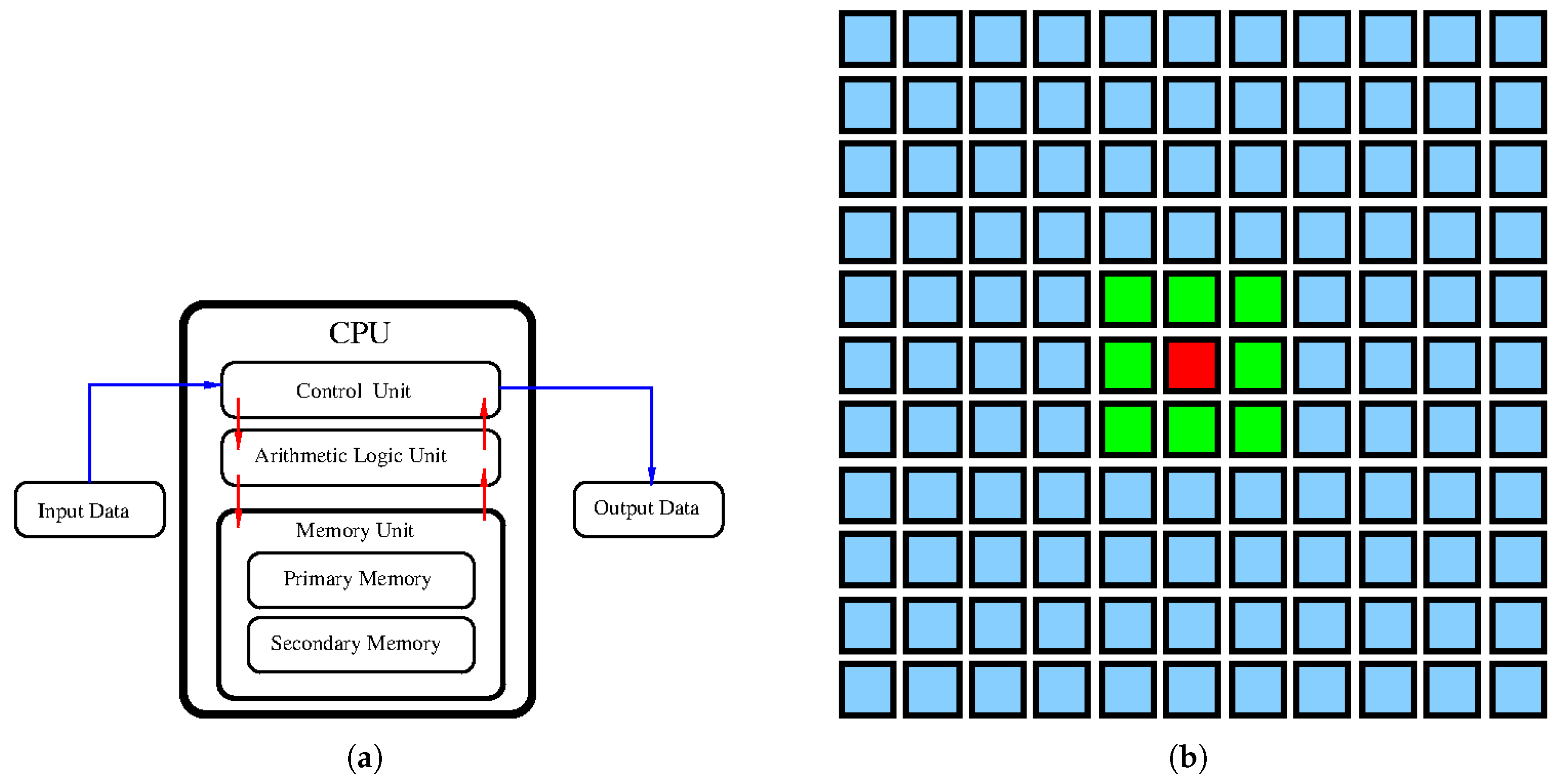
Figure 2.
Usually, a CA is designed using a two-dimensional lattice of squares. In 2D, there exist three different plane tillings: (a) The most commonly used is the square grid. It has a high anisotropy. (b) The hexagonal grid has the lowest anisotropy. (c) The triangular grid. Six neighboring triangles give one hexagon.
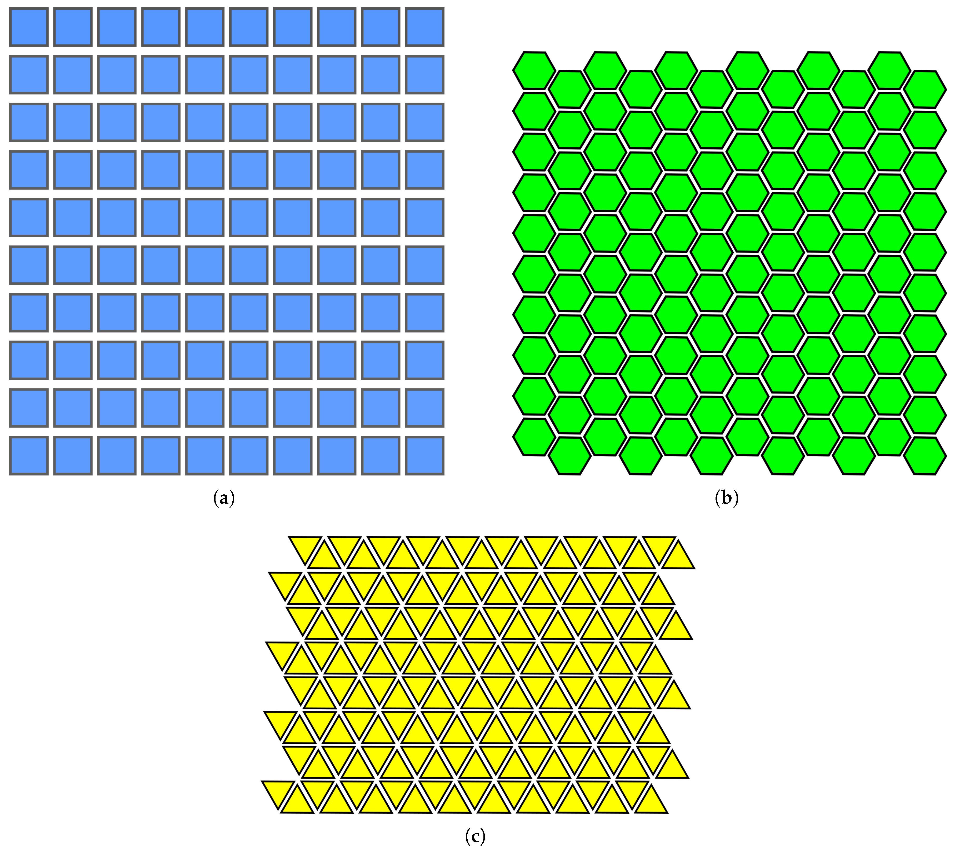
Figure 3.
Uniform and non-uniform networks are displayed in sub-figures (a) and (b), respectively. A uniform network is easier to program because its neighborhood and evolution rule are identical for each node.
Figure 3.
Uniform and non-uniform networks are displayed in sub-figures (a) and (b), respectively. A uniform network is easier to program because its neighborhood and evolution rule are identical for each node.
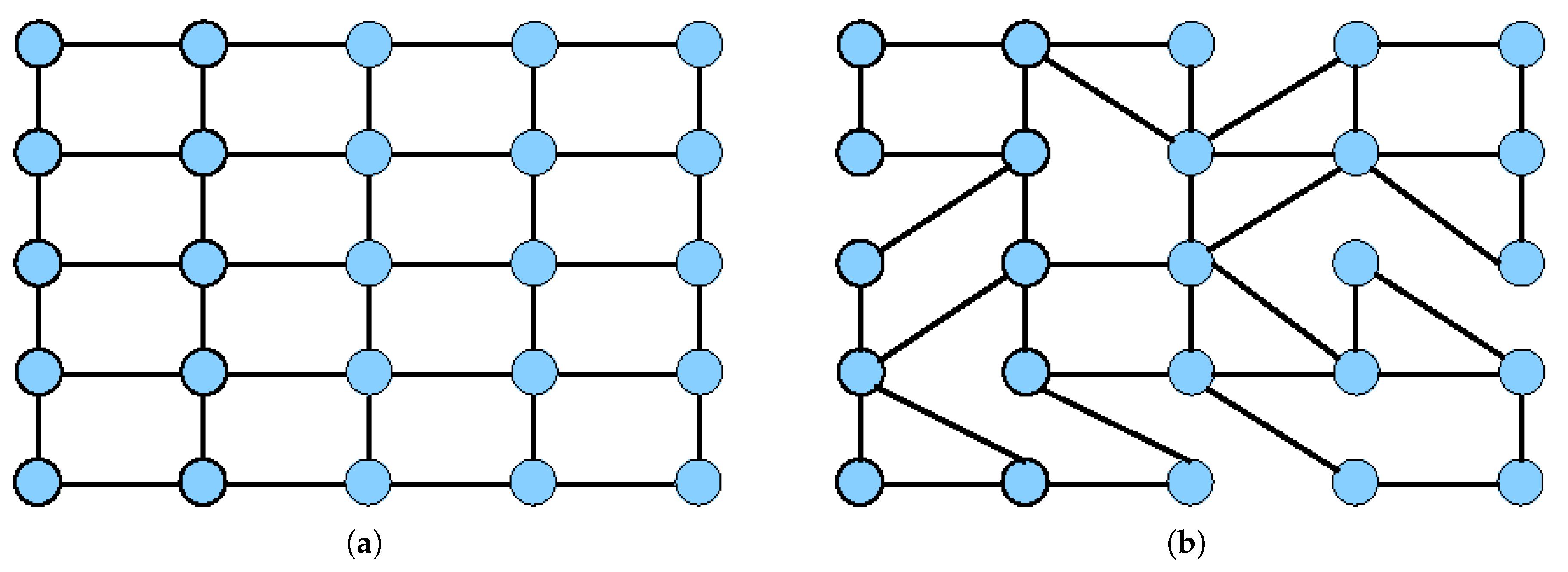
Figure 4.
A schematic depiction of a 1-D cellular automaton simulating a 1-D diffusion equation: steps before (a) and after (a) splitting of values of the only three central cells are depicted. In real simulations value splitting is much subtler. (a) The step BEFORE splitting of values within three cells. Values of red, green, and blue cells are split into three equal parts. (b) The step AFTER splitting of values within three cell. Three parts of red, green, and blue cells are split between left and right neighbors and the cell itself.
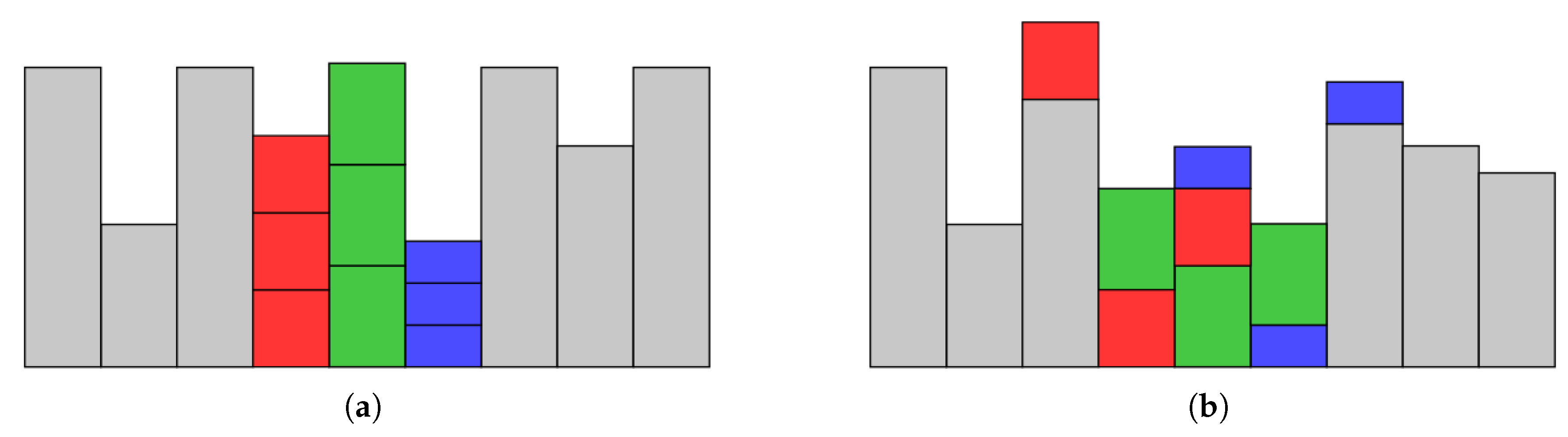
Figure 5.
Selected types of networks that are demonstrated on examples created above regularly spaced nodes; see definitions in [30,31]. Graphical representation of networks helps in their uderstanding. (a) Uniform networks link nodes regularly (equivalent to CAs). (b) Random networks link nodes randomly. (c) Small-world networks link the majority of nodes regularly and a the rest randomly. (d) Scale-free networks link nodes such that the node degree follows the power law.
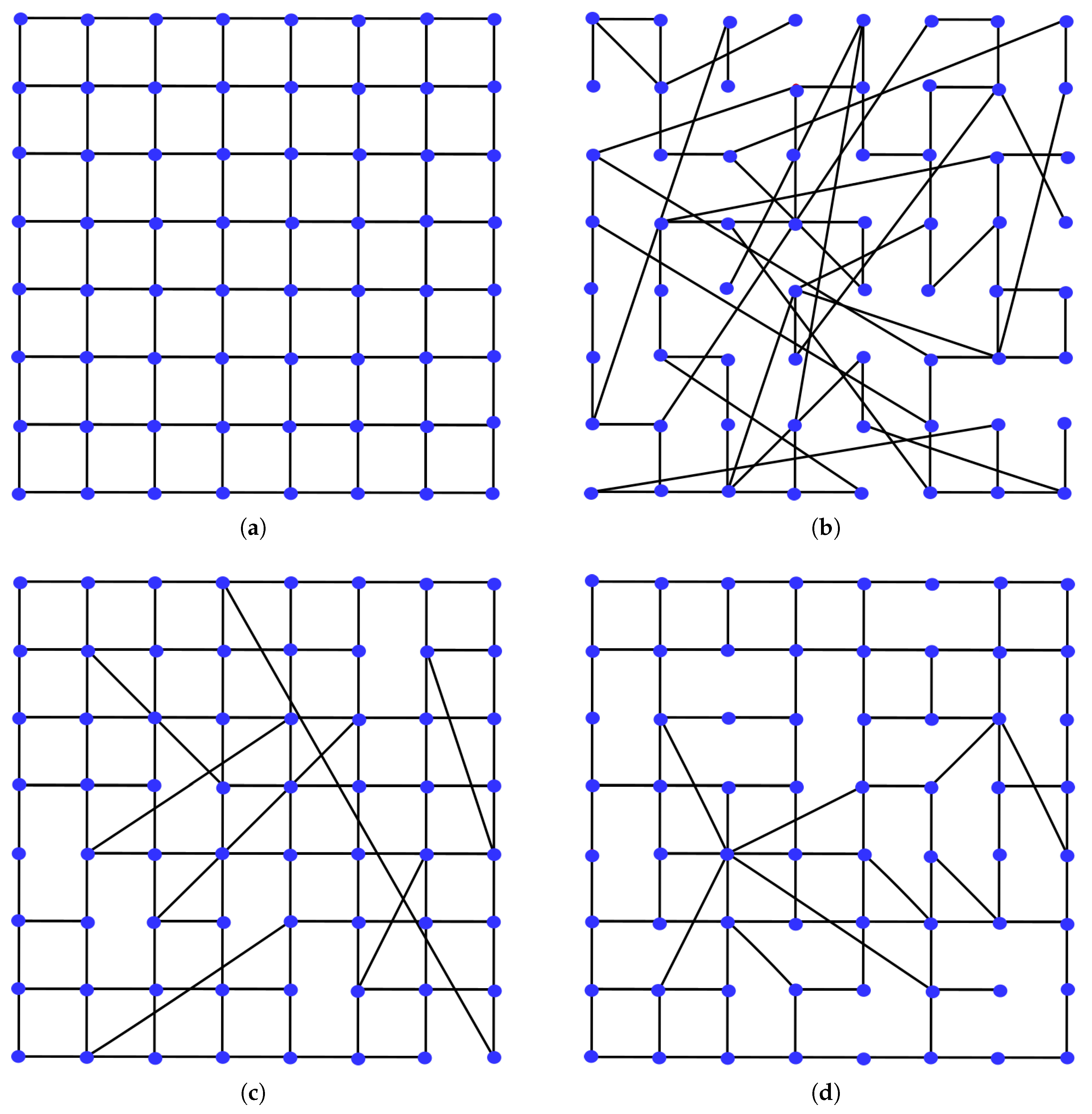
Figure 6.
Topology and Functioning of ad hoc graphs. (A) A set of agents. (B) The same set after a move where new positions are marked by red points and arrows. (a) The initial configuration of movable agents with the marked neighborhood of one agent (gray). (b( The updated configuration with the marked neighborhood of the same agent (pink).
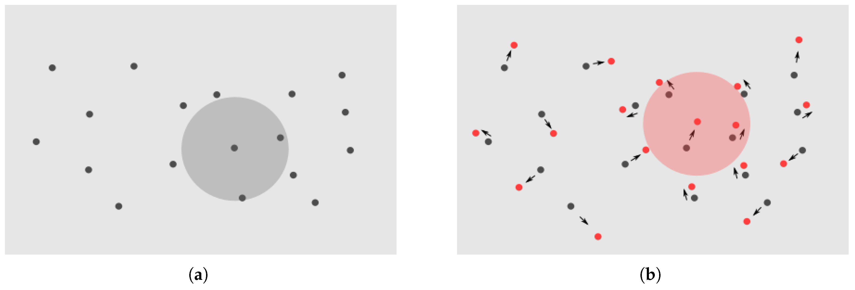
Figure 7.
A simulation of ships breeding ships: (A) initial random configuration, and (B–D) where both breeding-ships and trails of the second-order ships are present. Nothing is predefined (viz A). All emergents rise spontaneously from cells’ interactions (B–D). (a) Random initial conditions: rise of any meaningful emergent structure is not anticipated: at step 00. (b) A spontaneous emergence of the first, first-level breeding ship (the red circle), which is fast: step 05. (c) A breeding ship generate the first, second-level emergent ship (the red circle) that is slower: the step 16. This speed discrepancy eventually led to collisions due to periodic boundary conditions. (d) The rise of collisions (the red circle) between the first (top of the circle) and second order (bottom of the circle) ships due to overcrowding that is caused by periodic boundary conditions: step 93.
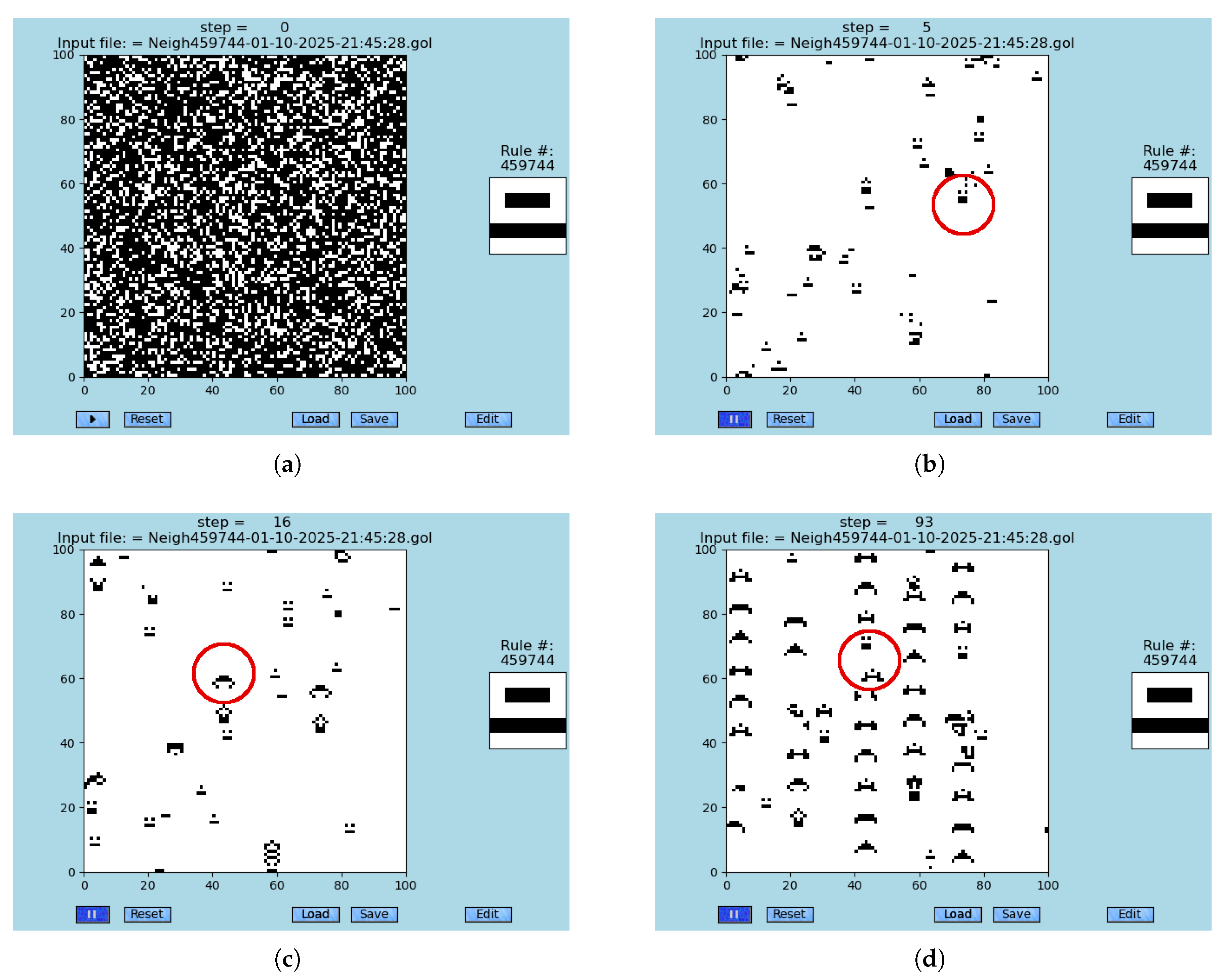
Figure 8.
Snapshots from the simulations of logic gate OR having the input of 11 and logic gate AND having the input of 11. (a) A simulation of a manually designed logic gate OR that is made of two input glider guns and two control glider guns that all are emitting gliders, and one blocker. (b) A simulation of manually designed logic gate AND with two input glider guns, one control glider gun that are emitting gliders, and one blocker.
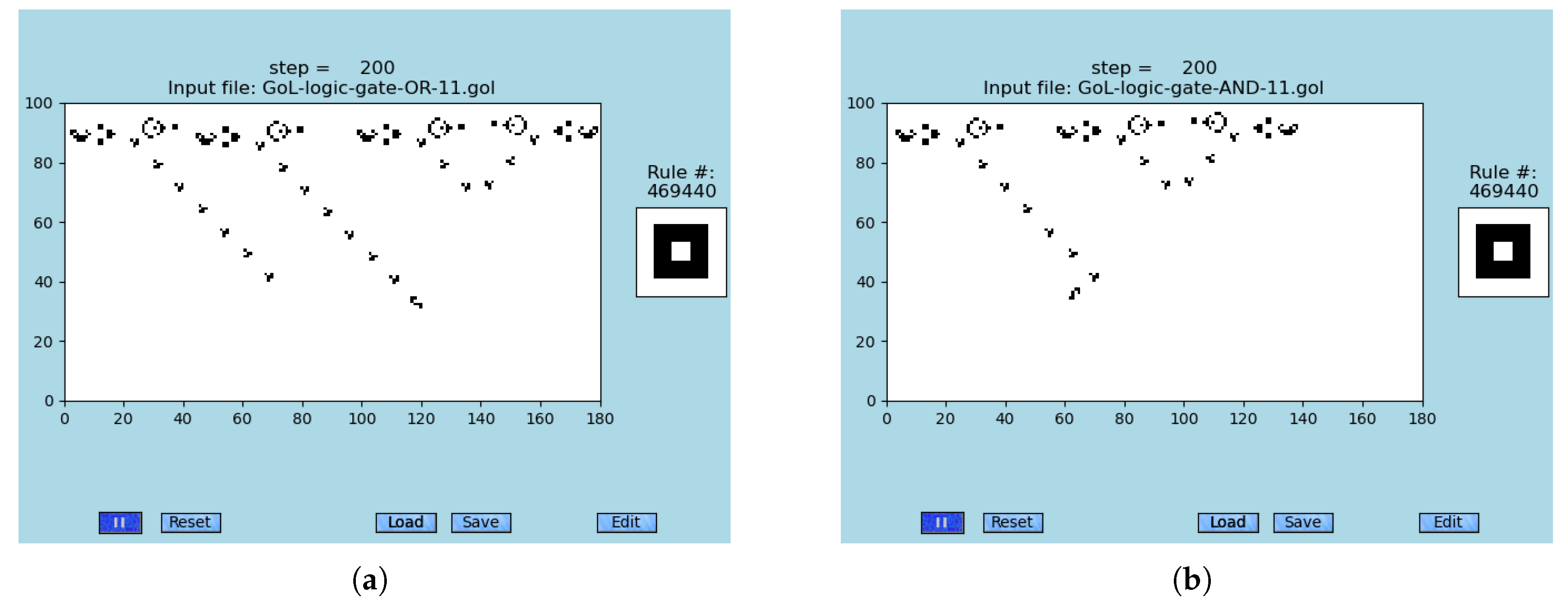
Figure 9.
Fast, long-range synchronization problem S2D-SP is partially error-resilient [13] (includes link to animations) and recovers from sporadic randomly injected errors. Seeds are spontaneously occurring in the majority of randomly initiated simulations. (a) Seeding configuration, time = 0. (b) Synchronized subsets, time = 46. (c) Synchronized subsets, time = 94. (d) The fully synchronized subset, time = 126.
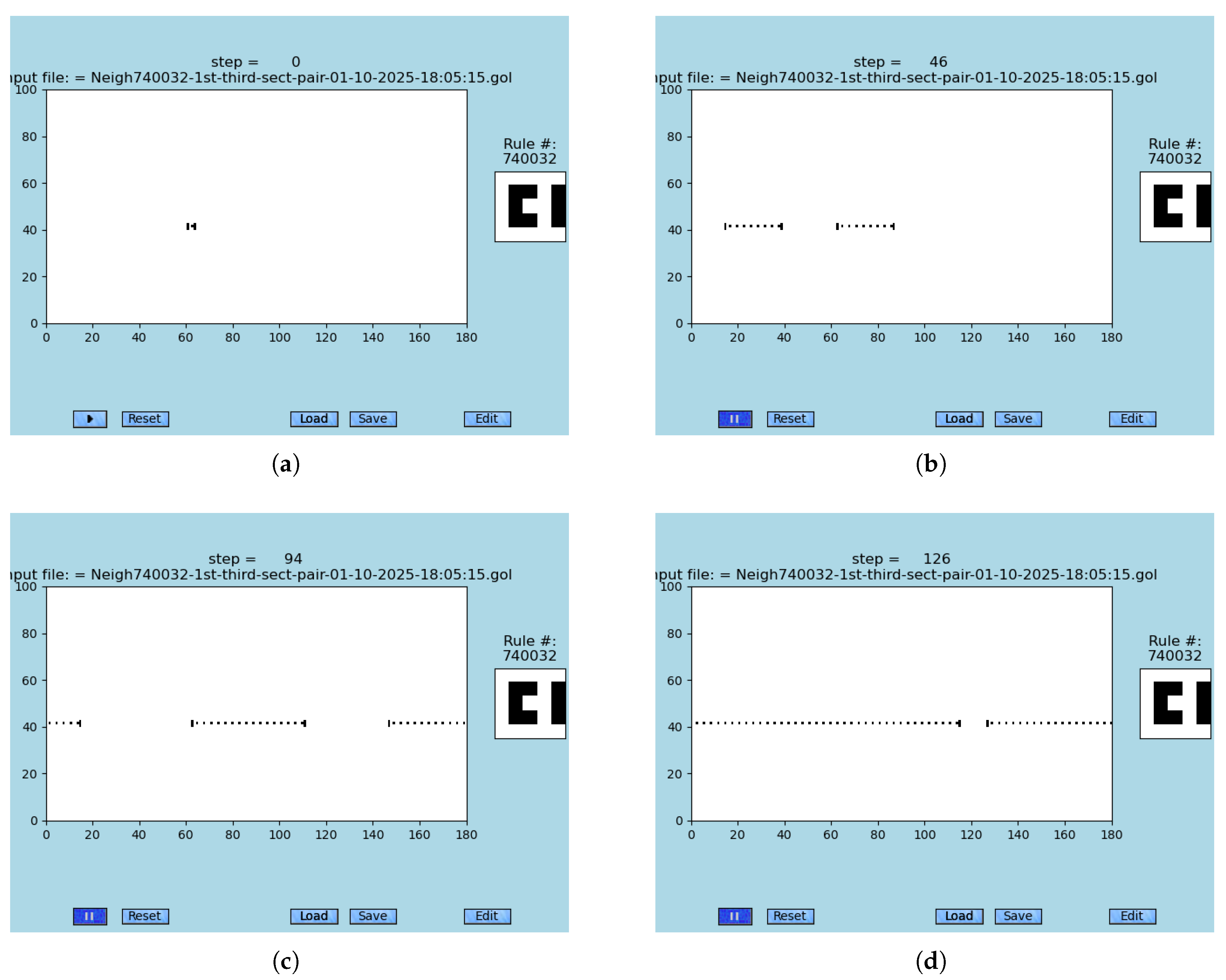

Table 1.
List of the major massively parallel (MP) techniques used in scientific computing with a brief description and citations. This review enables finding and diving into other MPC methods of interest.
Table 1.
List of the major massively parallel (MP) techniques used in scientific computing with a brief description and citations. This review enables finding and diving into other MPC methods of interest.
| MP Technique | Description |
|---|---|
| Cellular Automata (CA) | Micro-processes are operating above a fixed lattice (e.g., squares, triangles, or hexagons in 2-dimensions), discrete updating depends on a preselected neighborhood [6,7,8]. |
| Agent-Based Models (ABM) | Same as CAs except for freely moving agents that interact when they meet each other (no fixed neighborhood) [9]. |
| Lattice Gas Models (LGM) | LGMs treat gas as a matrix where each element contains many gas particles [10]. |
| Emergent Information Processing (EIP) | A generalized version of CAs where a limited number of neighbors is selected from a wider region [11,12,13]; see Section 7. |
| Multi-Scale Models (MSM) | MSMs incorporate several layers of models with increasing granularity, where each of the layers utilizes a different model (often an MP model is present in one of the scales) [14,15]. |
| Neuronal Networks (NN) | An iconic method of massively parallel computing. Many types of NN wiring, information propagation, and algorithms exist [16,17]. |
| Massively-Parallel Supercomputers (MPSP) | Modern supercomputers are based on massively-parallel distribution of computation [18], where many simpler computers are wired in networks. Specific problems require solutions using CSs, e.g., synchronization task; see Section 8. |
| Biological Computations (BC) | BCs include DNA computing [19,20], yeast cells computing [21], slime mold computing [22], protein folding, and others. |
| Graph Computing (GC) | GC utilizes graphs instead of lattices to perform computations; several methodologies could be applied, e.g., CAs, NNs, etc. |
| Graphic Cards | A substantial speed up of graphic computations is achieeved using graphic cards. |
Table 2.
The list of the major, generic types of networks along with their brief descriptions. The seminal review dealing with networks was provided by Albert & Barabási [30,31]. Often the identical network could belong to several classes simultaneously!
| Network Type | Description |
|---|---|
| Uniform Networks | Each node is connected uniformly to neighboring nodes via the identical neighborhood [30]. They represent the standard definition of CAs; see Section 2 and Figure 5 (A). |
| Random Networks | Links among nodes are chosen randomly. The number of links going from each node vary [30]; see Figure 5 (B). |
| Small-World Networks | Uniform networks in which a smaller number of links of a uniform network are reconnected randomly. For example, societal contacts are small-world networks [30]; see Figure 5 (C). |
| Scale-Free networks | They represent the networks that express self-similarity at many scales simultaneously; examples are networks of the Internet, WWW, metabolic, protein-protein interactions, semantic networks, and airline networks. Node degree distribution of scale-free networks follows the power law [30]; see Figure 5 (D). |
| Neural Networks | Networks of simplified, artificial ’neurons,’ mimic the behavior of real neural networks, that are observed in the human brain. |
| Static Networks | Networks that keep their shape unchanged during their entire existence. They are fixed in time. |
| Dynamic Networks | Those networks change their connection during their existence. They are flexibly adjusting to the needs of the system in time. |
| Ad Hoc Networks | They represent a subgroup of dynamic networks; see Figure 6 with agents. Their existence is defined by the actual topology of a given system. A prototypical example is given by interaction networks observed within structural components of living cells. |
Table 3.
Selected examples of hardware implementations of cellular automata that are used to accelerate their simulations.
Table 3.
Selected examples of hardware implementations of cellular automata that are used to accelerate their simulations.
| Type of Hardware | Authors |
|---|---|
| Cellular Automata Machines (CAM). | Tomasso Toffoli [34] |
| Hardware acceleration of CA simulations using graphic cards (GPUs). | Cagiggas-Muñiz, Diaz-del-Rio, López-Torres, Jiménez-Morales, and Guisado [36] |
| Photonic cellular automata simulating complex phenomena. | Li, Leefmans, Williams, and Marandi [35] |
| Energy-Efficient Hardware. | Morán, Frasser, Roca, and Rosselo [37] |
| CAs implemented using memristors. | Wang, H. and Wang, J. and Yan, S. et al. [38] |
| Cardiac hybrid cellular automata model using GPU. | Treml, Bartocci, and Gizzi [39] |
| Implementing cellular automata in FPGA logic. | Halbach and Hoffmann [40] |
| Reviews of hardware implementations of CAs. | Bakhteri [41], Dascalu [42], |
| Programmable hardware CA. | Charbouillot, Perez, and Fronte [43] |
| Cellular automata hardware implementation (review). | Sirakoulis [44] |
Table 4.
Examples of software and environments that are used to simulate cellular automata and agent-based models that are suitable for newcomers.
Table 4.
Examples of software and environments that are used to simulate cellular automata and agent-based models that are suitable for newcomers.
| Description of Software | Implementation |
|---|---|
| Simplest implementation of the GoL. | Open-source Python [33]. |
| Error-resilient CA: r-GoL (recovers from induced noise). | Open-source Python [45]. |
| Extended neighborhoods using implementation of GoL: GoL-N24. | Open-source Python [32]. |
| CelLab is exploring CAs using the WebCA simulator. | Closed software, enables design rule in JavaScript[46]. |
| Golly enables explorations of GoL and many other rules. | Open-source and cross-platform [47]. |
| StarLogo TNG is a multi-platform ABM environment used in the education of massively-parallel computing environments. | Downloadable software [48,49,50]. |
| NetLogo is an ABM programmable modeling environment used in research. | Available as a web-based environment or downloadable for Mac, Windows, and Linux [51]. |
Table 5.
Broad classes of computing devices and methods. At the top are macroscopic computers, and at the bottom are microscopic ones.
Table 5.
Broad classes of computing devices and methods. At the top are macroscopic computers, and at the bottom are microscopic ones.
| Computing Type | Description |
|---|---|
| Analog Computers | Uses continuous physical quantities to solve problems: water flow simulating economy, industrial processes, calculating integrals, fluidic algebraic machines (Archimedes), fluidic devices, fluid mappers [22,85], social insects [86,87], electromagnetism, etc. |
| Conventional Computing | Mainframe computers, supercomputers, PCs, processors having several cores, and embedded computers represent the most common form of currently used computers. |
| Unconventional Computing | Liquid computers [22], biocomputing [84,88], chemical computing [89,90], DNA computing [19,20], ... |
| Quantum Computing | A surprising interpretation of QM using massively-parallel computations implemented in CAs was found that opens gates to quantum computing; see the book by ’t Hooft [81]. (Are there operating processes originating in the noumenal realms?) |
| Photonic Computing | A novel approach of extremely fast computing [91,92,93]. |
| Emergent Information Processing (EIP) | Utilizes the components: a matrix, local neighborhood, and evolves using micro-processes operating in parallel above information provided by neighbors [11,12,13,29,32,33,45]. |
| Constituting Underlying Reality | It contains two basic components: unknown matrix and unknown micro-processes. Only indirect understanding exists; see Section 11.3 for details. |
Table 6.
Various authors and approaches describe observable and unobservable natural phenomena differently according to sensory inputs.
Table 6.
Various authors and approaches describe observable and unobservable natural phenomena differently according to sensory inputs.
| Author | Observable | Unobservable |
|---|---|---|
| Unknown | Seen Realms | Unseen Realms |
| Plato | Physics describes observed physical phenomena. | Metaphysics deals with processes beyond observations. |
| Immanuel Kant | Phenomenal knowledge is dependent on senses. | Noumenal knowledge is independent of senses. |
| Emergent Information Processing | Emergents are products of the observed emergent and self-organized phenomena. | Matrix + Micro-Evolution constitute the ground level of the system, which is hidden. |
Disclaimer/Publisher’s Note: The statements, opinions and data contained in all publications are solely those of the individual author(s) and contributor(s) and not of MDPI and/or the editor(s). MDPI and/or the editor(s) disclaim responsibility for any injury to people or property resulting from any ideas, methods, instructions or products referred to in the content. |
© 2025 by the authors. Licensee MDPI, Basel, Switzerland. This article is an open access article distributed under the terms and conditions of the Creative Commons Attribution (CC BY) license (http://creativecommons.org/licenses/by/4.0/).
Copyright: This open access article is published under a Creative Commons CC BY 4.0 license, which permit the free download, distribution, and reuse, provided that the author and preprint are cited in any reuse.


