Lie Symmetry Analysis and Invariant Solutions of the (1+1)-Dimensional Fisher Equation

1. Introduction

Reaction–diffusion equations form an essential mathematical framework for modelling spatial population dynamics, chemical kinetics, nerve propagation, and biological invasion phenomena [1,2]. In ecological and population genetics, they describe how local reaction mechanisms, such as growth and competition, interact with spatial diffusion to generate travelling fronts, invasion waves, and patterned structures [3].

One of the most classical and influential models of this class is the Fisher equation, introduced by Fisher in 1937 to describe the spread of an advantageous gene in a population [4] and independently developed by Kolmogorov, Petrovsky, and Piskunov in the same year [5]. In its general reaction–diffusion form, the Fisher (or Fisher–KPP) equation is written as

$${\displaystyle \frac{\partial u}{\partial t}}={\displaystyle \frac{{\partial }^{2}u}{\partial x^2}}+f\left(u\right),$$

(1)

where $u(x,t)$ denotes the population density, x is the spatial coordinate, and t is time. For the standard Fisher model, the nonlinear reaction term is logistic,

$$f\left(u\right)=u(1-u),$$

(2)

leading to the well–known logistic Fisher equation

$${\displaystyle \frac{\partial u}{\partial t}}={\displaystyle \frac{{\partial }^{2}u}{\partial x^2}}+u(1-u).$$

(3)

The Fisher equation admits travelling–wave solutions with sigmoidal profiles that describe the advance of a stable state into an unstable one, a phenomenon central to population genetics, ecology, and chemical propagation modelling [2,3]. Foundational discussions of travelling fronts and related biological applications can be found in Murray [2]. Explicit travelling–wave solutions for special parameter values, most notably the classical Ablowitz–Zeppetella solution, highlight the mathematical richness of the model [6]. Further insights into wave propagation and nonlinear diffusion have been presented in the works of Aronson and Weinberger [7], Feroe [8], and Zinner [9], among others.

Over the years, a variety of analytical and numerical techniques have been applied to Fisher–type equations. Loyinmi and Akinfe [10] obtained exact solutions for a family of Fisher reaction–diffusion equations using the Elzaki homotopy transformation method. Mittal and Jain [11] developed numerical solutions based on a modified cubic B–spline collocation scheme. Wavelet and spectral-type approaches for reaction–diffusion problems were reviewed by Hariharan and Kannan [12], while Salas et al. [13] investigated reaction–diffusion equations in a chemical context. More recently, Yang and Pan [14] constructed new solitary–wave solutions of the Fisher equation using a Riccati-type ansatz combined with direct algebraic techniques.

Lie symmetry analysis provides a rigorous and systematic framework for studying nonlinear differential equations by exploiting their invariance properties under continuous transformation groups. Classical references, including Arrigo [15], Bluman and Anco [16], Bluman and Kumei [17], Hydon [18], Ibragimov [19], and Ovsiannikov [20], establish the theoretical foundations of symmetry methods and their applications to reaction–diffusion models. For constructing exact travelling–wave solutions, tanh and extended tanh methods have been widely used in conjunction with symmetry reductions [21,22].

In this study, we conduct a Lie symmetry analysis of the one–dimensional Fisher reaction–diffusion equation. We determine its infinitesimal generators, derive similarity reductions, and solve the resulting reduced ordinary differential equations to obtain explicit invariant and travelling–wave solutions. The analysis illustrates the effectiveness of Lie symmetry techniques in producing analytically tractable and biologically meaningful solutions for Fisher–type reaction–diffusion systems.

2. Finding the Symmetries of the Fisher’s Equation

The Lie symmetry method determines the invariance of partial differential equations under continuous transformation groups, enabling systematic reductions to simpler forms [18]. In this section, we apply Lie symmetry analysis to the standard Fisher equation,

$${\displaystyle \frac{\partial u}{\partial t}}={\displaystyle \frac{{\partial }^{2}u}{\partial x^2}}+u(1-u).$$

We consider the infinitesimal transformations

$$\begin{array}{cc}\hfill x^{*}& =x+ϵ\xi (x,t,u)+\mathcal{O}\left({ϵ}^2\right),\hfill \end{array}$$

(4)

$$\begin{array}{cc}\hfill t^{*}& =t+ϵ\tau (x,t,u)+\mathcal{O}\left({ϵ}^2\right),\hfill \end{array}$$

(5)

$$\begin{array}{cc}\hfill u^{*}& =u+ϵ\eta (x,t,u)+\mathcal{O}\left({ϵ}^2\right),\hfill \end{array}$$

(6)

with the associated infinitesimal generator

$$X=\xi {\displaystyle \frac{\partial }{\partial x}}+\tau {\displaystyle \frac{\partial }{\partial t}}+\eta {\displaystyle \frac{\partial }{\partial u}}.$$

(7)

Using MAPLE and the PDEtools package, the infinitesimal functions for the Fisher equation were computed as

$$\begin{array}{c}\hfill \xi (x,t,u)=0,\tau (x,t,u)=1,\eta (x,t,u)=0,\end{array}$$

(8)

$$\begin{array}{c}\hfill \xi (x,t,u)=1,\tau (x,t,u)=0,\eta (x,t,u)=0.\end{array}$$

(9)

From these infinitesimals, we obtain the corresponding symmetry generators:

$$X_1={\displaystyle \frac{\partial }{\partial t}},X_2={\displaystyle \frac{\partial }{\partial x}}.$$

(10)

These generators represent time-translation and space-translation symmetries, respectively.

2.1. Commutator of the Symmetries

The infinitesimal generators

$$X_1={\displaystyle \frac{\partial }{\partial t}},X_2={\displaystyle \frac{\partial }{\partial x}}$$

are the two Lie point symmetries of the Fisher’s equation. The commutator (or Lie bracket) of two vector fields is defined as

$$[X_1,X_2]=X_1{X}_2-X_2{X}_1.$$

(11)

Since partial derivatives commute, we have

$${\displaystyle \frac{\partial }{\partial t}}\left({\displaystyle \frac{\partial }{\partial x}}\right)={\displaystyle \frac{\partial }{\partial x}}\left({\displaystyle \frac{\partial }{\partial t}}\right),$$

(12)

which implies that

$$[X_1,X_2]=0.$$

(13)

The vanishing of the commutator, $[X_1,X_2]=0$, shows that the two symmetries commute. This means:

• The order in which the symmetries are applied does not matter.
• The symmetry algebra generated by $X_1$ and $X_2$ is Abelian.
• These symmetries may be used independently to reduce the PDE, or in combination (e.g., as a linear combination for a travelling–wave variable $z=x-ct$).

2.2. Invariant Solution Using $X_1={\partial }_t$

We seek an invariant solution under the Lie point symmetry generator

$$X_1={\displaystyle \frac{\partial }{\partial t}}.$$

(14)

This symmetry corresponds to invariance under time translations. To find an invariant solution, we use the method of characteristics. The associated characteristic system is

$${\displaystyle \frac{dx}{0}}={\displaystyle \frac{dt}{1}}={\displaystyle \frac{du}{0}}.$$

(15)

We get the two invariants

$$T_1=x\mathrm{and}{T}_2=u,$$

(16)

and the group–invariant solution is given by

$$T_2=f\left(T_1\right),\mathrm{i}.\mathrm{e}.,u=f\left(x\right).$$

(17)

Hence, the invariant solution takes the form

$$u(x,t)=f\left(x\right).$$

(18)

We now substitute the invariant form $u(x,t)=f\left(x\right)$ into Fisher’s equation

$${\displaystyle \frac{\partial u}{\partial t}}={\displaystyle \frac{{\partial }^{2}u}{\partial x^2}}+u(1-u).$$

(19)

Since u depends only on x, the time derivative vanishes,

$${\displaystyle \frac{\partial u}{\partial t}}=0.$$

(20)

The spatial derivatives become

$${\displaystyle \frac{\partial u}{\partial x}}=f^{\prime }\left(x\right),{\displaystyle \frac{{\partial }^{2}u}{\partial x^2}}=f^{\prime \prime }\left(x\right).$$

(21)

Substituting these gives

$$f^{\prime \prime }\left(x\right)+f\left(x\right)\left(1-f\left(x\right)\right)=0.$$

(22)

The reduced Equation is a nonlinear second–order equation and cannot be solved using standard techniques such as separation of variables, integrating factors, or other familiar methods for linear ODEs. Nonlinear equations of this form are difficult to handle analytically and require specialised approaches. In this work, we attempt to obtain an exact solution using the Tanh method.

We apply the tanh method by introducing the transformation

$$T=tanh\left(kx\right),$$

(23)

where $k\ne 0$. Since

$${\displaystyle \frac{dT}{dx}}=k(1-T^2),$$

(24)

this substitution allows derivatives of f to be rewritten in terms of T. A balance of the highest powers in the ODE shows that the solution should take the form of a quadratic polynomial in T, so we assume

$$f\left(x\right)=a_0+a_{1}T+a_2{T}^2,$$

(25)

where $a_0,a_1,a_2$ and k are constants to be determined.

Differentiating the ansatz using the chain rule gives

$$f^{\prime }\left(x\right)={\displaystyle \frac{df}{dT}}{\displaystyle \frac{dT}{dx}}=(a_1+2a_{2}T)k(1-T^2).$$

(26)

Differentiating again, we set

$$g\left(T\right)=(a_1+2a_{2}T)(1-T^2),$$

(27)

so that

$$f^{\prime \prime }\left(x\right)=k^2{g}^{\prime }\left(T\right)(1-T^2).$$

(28)

Computing $g^{\prime }\left(T\right)$ gives

$$g^{\prime }\left(T\right)=2a_2-2a_{1}T-6a_2{T}^2.$$

(29)

Therefore, the second derivative becomes

$$f^{\prime \prime }\left(x\right)=k^2(2a_2-2a_{1}T-6a_2{T}^2)(1-T^2),$$

(30)

and expanding yields

$$f^{\prime \prime }\left(x\right)=k^2\left(6a_2{T}^4+2a_1{T}^3-8a_2{T}^2-2a_{1}T+2a_2\right).$$

(31)

Next, we expand the nonlinear reaction term. Substituting the polynomial ansatz gives

$$f(1-f)=(a_0-a_0^2)+(a_1-2a_0{a}_1)T+(-2a_0{a}_2-a_1^2+a_2)T^2-2a_1{a}_2{T}^3-a_2^2{T}^4.$$

(32)

Substituting the expressions for $f^{\prime \prime }\left(x\right)$ and $f(1-f)$ into the reduced ODE

$$f^{\prime \prime }+f(1-f)=0,$$

(33)

and simplifying gives

$$\begin{array}{cc}\hfill k^2(6a_2{T}^4+2a_1{T}^3-8a_2{T}^2-2a_{1}T+2a_2)+(a_0-a_0^2)+(a_1-2a_0{a}_1)T& \hfill \\ \hfill +(-2a_0{a}_2-a_1^2+a_2)T^2-2a_1{a}_2{T}^3-a_2^2{T}^4& =0.\hfill \end{array}$$

(34)

Equating coefficients of like powers of T gives the algebraic system:

$$\begin{array}{cc}\hfill T^4:& 6a_2{k}^2-a_2^2=0,\hfill \end{array}$$

(35)

$$\begin{array}{cc}\hfill T^3:& 2a_1{k}^2-2a_1{a}_2=0,\hfill \end{array}$$

(36)

$$\begin{array}{cc}\hfill T^2:& -8a_2{k}^2-2a_0{a}_2-a_1^2+a_2=0,\hfill \end{array}$$

(37)

$$\begin{array}{cc}\hfill T^1:& -2a_1{k}^2+a_1-2a_0{a}_1=0,\hfill \end{array}$$

(38)

$$\begin{array}{cc}\hfill T^0:& 2a_2{k}^2+a_0-a_0^2=0.\hfill \end{array}$$

(39)

Solving begins with the first condition

$$a_2(6k^2-a_2)=0.$$

(40)

If $a_2=0$, then

$$2a_1{k}^2=0\Rightarrow a_1=0,$$

(41)

and the constant–term equation

$$a_0-a_0^2=0$$

(42)

gives the two equilibrium solutions

$$f=0,f=1.$$

(43)

To obtain a nonconstant solution we take $a_2=6k^2$. Substituting into

$$2a_1{k}^2-2a_1{a}_2=0$$

(44)

gives

$$2a_1(k^2-6k^2)=-10k^2{a}_1=0,$$

(45)

so

$$a_1=0.$$

(46)

Using $a_1=0$ and $a_2=6k^2$ in the quadratic condition

$$-8a_2{k}^2-2a_0{a}_2+a_2=0$$

(47)

yields

$$-48k^4-12a_0{k}^2+6k^2=0.$$

(48)

Dividing by $6k^2$ gives

$$-8k^2-2a_0+1=0,$$

(49)

hence

$$a_0={\displaystyle \frac{1-8k^2}{2}}.$$

(50)

Substituting into the final condition

$$2a_2{k}^2+a_0-a_0^2=0$$

(51)

leads to

$$12k^4+{\displaystyle \frac{1-8k^2}{2}}-{\left({\displaystyle \frac{1-8k^2}{2}}\right)}^2=0.$$

(52)

Multiplying by 4 and simplifying gives

$$-1+16k^4=0,$$

(53)

so

$$k^2={\displaystyle \frac{1}{4}}.$$

(54)

Substituting back gives

$$a_2=6k^2={\displaystyle \frac{3}{2}},a_1=0,a_0=-{\displaystyle \frac{1}{2}}.$$

(55)

Hence the polynomial becomes

$$f\left(x\right)=a_0+a_2{T}^2=-{\displaystyle \frac{1}{2}}+{\displaystyle \frac{3}{2}}{T}^2.$$

(56)

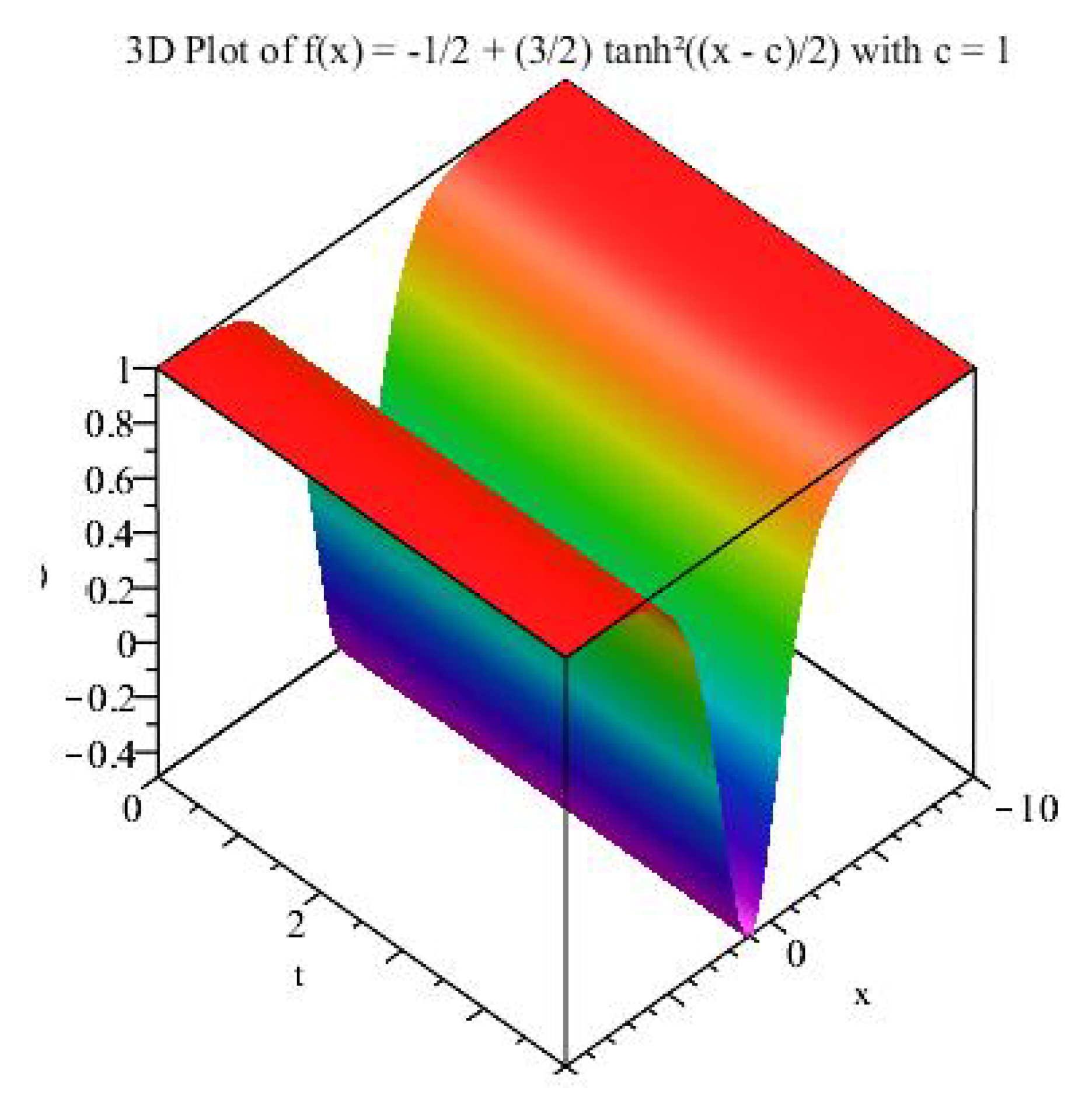
With $T=tanh\left(kx\right)$ and $k={\displaystyle \frac{1}{2}}$, we obtain the explicit invariant solution

$$f\left(x\right)=-{\displaystyle \frac{1}{2}}+{\displaystyle \frac{3}{2}}{tanh}^2\left({\displaystyle \frac{x}{2}}\right).$$

(57)

Since the reduced ODE is autonomous, a translation in x produces the one–parameter family

$$f\left(x\right)=-{\displaystyle \frac{1}{2}}+{\displaystyle \frac{3}{2}}{tanh}^2\left({\displaystyle \frac{x-x_0}{2}}\right),$$

(58)

where $x_0$ is a translation constant.

Figure 1. 3D Steady-State Invariant Solution Surface Corresponding to $X_1={\partial }_t$.

Figure 1. 3D Steady-State Invariant Solution Surface Corresponding to $X_1={\partial }_t$.

2.3. Invariant Solution Using $X_2={\partial }_x$

We seek an invariant solution under the Lie point symmetry generator

$$X_2={\displaystyle \frac{\partial }{\partial x}}.$$

(59)

This symmetry corresponds to invariance under spatial translations. To find an invariant solution, we use the method of characteristics. The associated characteristic system is

$${\displaystyle \frac{dx}{1}}={\displaystyle \frac{dt}{0}}={\displaystyle \frac{du}{0}}.$$

(60)

We obtain the two invariants

$$T_1=t\mathrm{and}{T}_2=u,$$

(61)

and the group–invariant solution is given by

$$T_2=f\left(T_1\right),\mathrm{i}.\mathrm{e}.u=f\left(t\right).$$

(62)

Hence, the invariant solution takes the form

$$u(x,t)=f\left(t\right).$$

(63)

We substitute the invariant form $u(x,t)=f\left(t\right)$ into the Fisher’s equation,

$${\displaystyle \frac{\partial u}{\partial t}}={\displaystyle \frac{{\partial }^{2}u}{\partial x^2}}+u(1-u).$$

Since u depends only on t, all spatial derivatives vanish

$${\displaystyle \frac{\partial u}{\partial x}}=0,{\displaystyle \frac{{\partial }^{2}u}{\partial x^2}}=0.$$

(64)

Hence, the PDE reduces to the ODE

$${\displaystyle \frac{df}{dt}}=f(1-f),$$

(65)

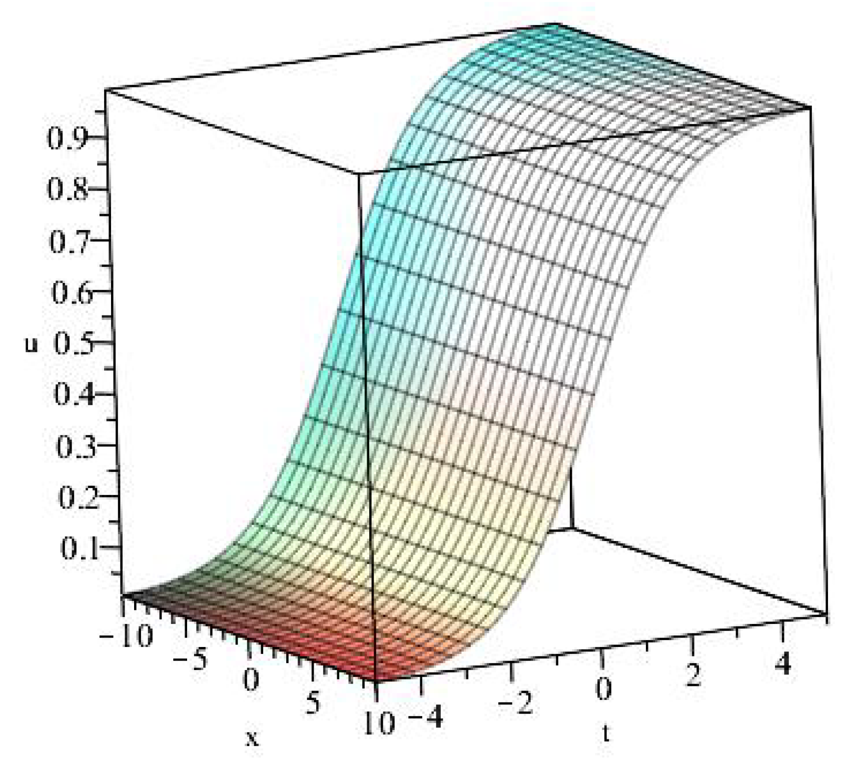
which is the logistic equation. Solving this equation using separation of variables, we obtain the explicit solution,

$$f\left(t\right)={\displaystyle \frac{1}{1+C_1{e}^{-t}}}.$$

(66)

where $C_1$ is an arbitrary constant of integration.

This solution represents a spatially uniform logistic growth model. As time progresses, the population density $u\left(t\right)$ increases and asymptotically approaches the equilibrium value $u=1$.

Figure 2. 3D Logistic Growth Surface Corresponding to the Symmetry $X_2={\partial }_x$

Figure 2. 3D Logistic Growth Surface Corresponding to the Symmetry $X_2={\partial }_x$

2.4. Invariant Solution Using The Travelling-Wave Symmetry $X={\partial }_t+c{\partial }_x$

We seek an invariant solution under the Lie point symmetry generator

$$X={\displaystyle \frac{\partial }{\partial t}}+c{\displaystyle \frac{\partial }{\partial x}}.$$

(67)

This symmetry corresponds to invariance under a travelling–wave transformation. To find an invariant solution, we use the method of characteristics. The associated characteristic system is

$${\displaystyle \frac{dt}{1}}={\displaystyle \frac{dx}{c}}={\displaystyle \frac{du}{0}}.$$

(68)

We obtain the two invariants

$$T_1=z=x-ct\mathrm{and}{T}_2=u,$$

(69)

and the group–invariant solution is given by

$$T_2=f\left(T_1\right),\mathrm{i}.\mathrm{e}.u(x,t)=f(x-ct).$$

(70)

Hence, the invariant variable is,

$$z=x-ct,$$

(71)

and the solution can be written as

$$u(x,t)=f\left(z\right).$$

(72)

We substitute the invariant form $u(x,t)=f\left(z\right)$, with $z=x-ct$, into Fisher’s equation

$${\displaystyle \frac{\partial u}{\partial t}}={\displaystyle \frac{{\partial }^{2}u}{\partial x^2}}+u(1-u).$$

(73)

Using the chain rule

$${\displaystyle \frac{\partial u}{\partial t}}={\displaystyle \frac{df}{dz}}{\displaystyle \frac{\partial z}{\partial t}}=-c{f}^{\prime }\left(z\right),$$

(74)

$${\displaystyle \frac{{\partial }^{2}u}{\partial x^2}}={\displaystyle \frac{d^{2}f}{d{z}^2}}.$$

(75)

Substituting these into the PDE yields,

$$f^{\prime \prime }\left(z\right)+c{f}^{\prime }\left(z\right)+f\left(z\right)(1-f\left(z\right))=0.$$

(76)

To obtain an exact solution of the nonlinear ODE

$$f^{\prime \prime }\left(z\right)+c{f}^{\prime }\left(z\right)+f\left(z\right)(1-f\left(z\right))=0,$$

we apply the tanh method. The idea is to express the solution in terms of a polynomial in the hyperbolic tangent function. We introduce the transformation

$$T=tanh\left(kz\right),$$

(77)

where $k\ne 0$. Since

$${\displaystyle \frac{dT}{dz}}=k(1-T^2),$$

(78)

this substitution allows the derivatives of f to be rewritten in terms of T. A balance of the highest powers in the ODE shows that the solution should take the form of a quadratic polynomial in T, so we assume

$$f\left(z\right)=a_0+a_{1}T+a_2{T}^2,$$

(79)

where $a_0,a_1,a_2$ and k are constants to be determined.

Differentiating the ansatz using the chain rule gives

$$f^{\prime }\left(z\right)={\displaystyle \frac{df}{dT}}{\displaystyle \frac{dT}{dz}}=(a_1+2a_{2}T)k(1-T^2).$$

(80)

Differentiating again, we set

$$g\left(T\right)=(a_1+2a_{2}T)(1-T^2),$$

(81)

so that

$$f^{\prime \prime }\left(z\right)=k^2{g}^{\prime }\left(T\right)(1-T^2).$$

(82)

Computing $g^{\prime }\left(T\right)$ gives

$$g^{\prime }\left(T\right)=2a_2-2a_{1}T-6a_2{T}^2.$$

(83)

Therefore, the second derivative becomes

$$f^{\prime \prime }\left(z\right)=k^2(2a_2-2a_{1}T-6a_2{T}^2)(1-T^2),$$

(84)

and expanding yields

$$f^{\prime \prime }\left(z\right)=k^2(6a_2{T}^4+2a_1{T}^3-8a_2{T}^2-2a_{1}T+2a_2).$$

(85)

Next, we expand the nonlinear reaction term. Substituting the polynomial ansatz gives

$$f(1-f)=(a_0-a_0^2)+(a_1-2a_0{a}_1)T+(-2a_0{a}_2-a_1^2+a_2)T^2-2a_1{a}_2{T}^3-a_2^2{T}^4.$$

(86)

For later use, we also write $f^{\prime }\left(z\right)$ in expanded form as

$$f^{\prime }\left(z\right)=k(a_1+2a_{2}T)(1-T^2)=k(-2a_2{T}^3-a_1{T}^2+2a_{2}T+a_1).$$

(87)

Substituting the expressions for $f^{\prime \prime }\left(z\right)$, $c{f}^{\prime }\left(z\right)$, and $f(1-f)$ into the ODE

$$f^{\prime \prime }+c{f}^{\prime }+f(1-f)=0$$

(88)

gives

$$\begin{array}{cc}\hfill k^2(6a_2{T}^4+2a_1{T}^3-8a_2{T}^2-2a_{1}T+2a_2)& +ck(-2a_2{T}^3-a_1{T}^2+2a_{2}T+a_1)\hfill \\ \hfill & +(a_0-a_0^2)+(a_1-2a_0{a}_1)T\hfill \\ \hfill & +(-2a_0{a}_2-a_1^2+a_2)T^2-2a_1{a}_2{T}^3-a_2^2{T}^4=0.\hfill \end{array}$$

(89)

Collecting like powers of T yields a polynomial identity

$$A_4{T}^4+A_3{T}^3+A_2{T}^2+A_{1}T+A_0=0,$$

(90)

where

$$\begin{array}{cc}\hfill A_4& =6a_2{k}^2-a_2^2,\hfill \end{array}$$

(91)

$$\begin{array}{cc}\hfill A_3& =2a_1{k}^2-2a_1{a}_2-2a_{2}ck,\hfill \end{array}$$

(92)

$$\begin{array}{ccc}\hfill A_2& =-8a_2{k}^2-2a_0{a}_2-a_1^2-a_{1}ck+a_2,A_1\hfill & \hfill =-2a_1{k}^2-2a_0{a}_1+a_1+2a_{2}ck,\end{array}$$

(93)

$$\begin{array}{cc}\hfill A_0& =2a_2{k}^2-a_0^2+a_0+a_{1}ck.\hfill \end{array}$$

(94)

Since this identity must hold for every value of T, the coefficients must vanish:

$$\begin{array}{cc}\hfill T^4:& 6a_2{k}^2-a_2^2=0,\hfill \end{array}$$

(95)

$$\begin{array}{cc}\hfill T^3:& 2a_1{k}^2-2a_1{a}_2-2a_{2}ck=0,\hfill \end{array}$$

(96)

$$\begin{array}{cc}\hfill T^2:& -8a_2{k}^2-2a_0{a}_2-a_1^2-a_{1}ck+a_2=0,\hfill \end{array}$$

(97)

$$\begin{array}{cc}\hfill T^1:& -2a_1{k}^2-2a_0{a}_1+a_1+2a_{2}ck=0,\hfill \end{array}$$

(98)

$$\begin{array}{cc}\hfill T^0:& 2a_2{k}^2-a_0^2+a_0+a_{1}ck=0.\hfill \end{array}$$

(99)

Solving these equations begins with the first condition,

$$a_2(6k^2-a_2)=0,$$

(100)

which gives either $a_2=0$ or $a_2=6k^2$.

Case 1: $a_2=0$

Then the second equation reduces to

$$2a_1{k}^2=0\Rightarrow a_1=0,$$

(101)

and the last equation becomes

$$-a_0^2+a_0=0,$$

(102)

so $a_0=0$ or $a_0=1$. These yield the constant solutions

$$f\left(z\right)=0,f\left(z\right)=1,$$

(103)

which are not travelling waves.

Case 2: $a_2=6k^2$

Substitute into the third-power condition

$$2a_1{k}^2-2a_1{a}_2-2a_{2}ck=0$$

(104)

$$\Rightarrow -10a_1{k}^2-12c{k}^3=0.$$

(105)

Dividing gives

$$5a_1+6ck=0,$$

(106)

and hence

$$a_1=-{\displaystyle \frac{6}{5}}ck.$$

(107)

Using these in the linear equation yields

$${\displaystyle \frac{6}{5}}ck(2a_0+12k^2-1)=0.$$

(108)

Assuming $c\ne 0$, $k\ne 0$,

$$2a_0+12k^2-1=0,$$

(109)

so

$$a_0={\displaystyle \frac{1-12k^2}{2}}.$$

(110)

Substituting $a_0,a_1,a_2$ into the quadratic condition reduces to

$$100k^2-c^2=0,$$

(111)

so

$$c^2=100k^2.$$

(112)

Finally, the constant-term equation becomes

$$(24k^2-1)(24k^2+1)=0.$$

(113)

Thus,

$$k^2={\displaystyle \frac{1}{24}},$$

(114)

and

$$k={\displaystyle \frac{1}{2\sqrt{6}}},c^2=100k^2={\displaystyle \frac{25}{6}}.$$

(115)

Taking $c>0$ for a right-moving wave gives

$$c={\displaystyle \frac{5}{\sqrt{6}}}.$$

(116)

The coefficients are then

$$a_2=6k^2={\displaystyle \frac{1}{4}},a_0={\displaystyle \frac{1-12k^2}{2}}={\displaystyle \frac{1}{4}},a_1=-{\displaystyle \frac{1}{2}}.$$

(117)

Hence, the polynomial becomes

$$f\left(z\right)=a_0+a_{1}T+a_2{T}^2={\displaystyle \frac{1}{4}}-{\displaystyle \frac{1}{2}}T+{\displaystyle \frac{1}{4}}{T}^2={\displaystyle \frac{1}{4}}{(1-T)}^2,$$

(118)

with

$$T=tanh\left({\displaystyle \frac{z}{2\sqrt{6}}}\right).$$

(119)

Therefore, the explicit nonconstant travelling–wave solution of the ODE is

$$f\left(z\right)={\displaystyle \frac{1}{4}}{\left[1-tanh\left({\displaystyle \frac{z}{2\sqrt{6}}}\right)\right]}^2.$$

(120)

Since the reduced ODE is autonomous, a translation in z also produces a solution. Thus,

$$f\left(z\right)={\displaystyle \frac{1}{4}}{\left[1-tanh\left({\displaystyle \frac{z-z_0}{2\sqrt{6}}}\right)\right]}^2,$$

(121)

where $z_0$ is a translation constant.

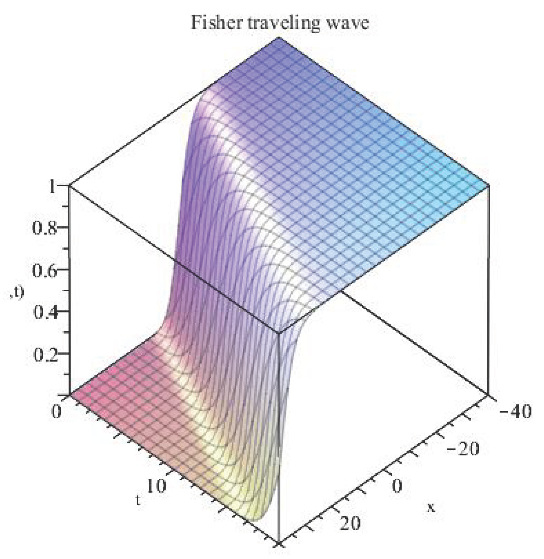
The obtained solution represents a travelling wave that connects the steady states $u=1$ and $u=0$. It describes a smooth transition front moving to the right with constant speed $c={\displaystyle \frac{5}{\sqrt{6}}}$. The solution models the propagation of a stable population invading an unstable region, with the wave maintaining its shape as it travels.

Figure 3. 3D plot of the Fisher travelling–wave solution, showing the wave front propagating in the positive x-direction.

Figure 3. 3D plot of the Fisher travelling–wave solution, showing the wave front propagating in the positive x-direction.

3. Conclusion

In this work, we applied Lie symmetry analysis to the one-dimensional Fisher reaction–diffusion equation and derived the corresponding symmetry reductions leading to invariant and travelling–wave solutions. The identified point symmetries enabled the systematic transformation of the governing PDE into reduced ODEs, which were solved explicitly to obtain closed-form wavefront profiles. These solutions capture the qualitative behaviour of propagating fronts commonly associated with Fisher-type models. The study demonstrates that Lie symmetry methods provide an effective analytical framework for simplifying nonlinear reaction–diffusion equations and extracting biologically meaningful travelling-wave solutions, offering valuable insight into the dynamics of invasion and population spread.

References

- Turing, A.M. The chemical basis of morphogenesis. Philosophical Transactions of the Royal Society of London B 1952, 237, 37–72. [Google Scholar]
- Murray, J.D. Mathematical Biology I: An Introduction, 3rd ed.; Springer: Berlin, 2007. [Google Scholar]
- Cosner, C. Reaction–diffusion equations and ecological modeling. In Tutorials in Mathematical Biosciences IV: Evolution and Ecology; Springer, 2008; pp. 77–115. [Google Scholar]
- Fisher, R.A. The wave of advance of advantageous genes. Annals of Eugenics 1937, 7(4), 355–369. [Google Scholar] [CrossRef]
- Kolmogorov, A.; Petrovsky, I.; Piskunov, N. Étude de l’équation de la diffusion avec croissance de la quantité de matière et son application à un problème biologique. Moscou Univ. Math. Bull. 1937, 1, 1–25. [Google Scholar]
- Ablowitz, M.J.; Zeppetella, A. Explicit solutions of Fisher’s equation for a special wave speed. Bulletin of Mathematical Biology 1979, 41(6), 835–840. [Google Scholar] [CrossRef]
- Aronson, D.G.; Weinberger, H.F. Nonlinear diffusion in population genetics, combustion, and nerve pulse propagation. In Partial Differential Equations and Related Topics; Springer, 1975; pp. 5–49. [Google Scholar]
- Feroe, J.A. Travelling wave solutions of the Nagumo equation. SIAM Journal on Applied Mathematics 1982, 42(2), 235–248. [Google Scholar] [CrossRef]
- Zinner, B. Existence of traveling wavefront solutions for the discrete Nagumo equation. Journal of Differential Equations 1992, 96(1), 1–27. [Google Scholar] [CrossRef]
- Loyinmi, A.C.; Akinfe, T.K. Exact solutions to the family of Fisher’s reaction–diffusion equation using Elzaki homotopy transformation perturbation method. Engineering Reports 2020, 2(2), e12084. [Google Scholar] [CrossRef]
- Mittal, R.C.; Jain, R.K. Numerical solutions of nonlinear Fisher’s reaction–diffusion equation with modified cubic B–spline collocation method. Mathematical Sciences 2013, 7(1), 12. [Google Scholar] [CrossRef]
- Hariharan, G.; Kannan, K. Review of wavelet methods for the solution of reaction–diffusion problems in science and engineering. Applied Mathematical Modelling 2014, 38(3), 799–813. [Google Scholar] [CrossRef]
- Salas, A.H.; Martínez, L.J.; Fernández, O. Reaction–diffusion equations: a chemical application. Scientia et Technica 2010, 3(46), 134–137. [Google Scholar]
- Yang, Z.; Pan, H. New solitary wave solutions of the Fisher equation. Journal of Applied Mathematics and Physics 2022, 10(11), 3356–3368. [Google Scholar] [CrossRef]
- Arrigo, D.J. Symmetry Analysis of Differential Equations: An Introduction; John Wiley & Sons, 2015. [Google Scholar]
- Bluman, G.; Anco, S. Symmetry and Integration Methods for Differential Equations; Springer Science & Business Media, 2008; volume 154. [Google Scholar]
- Bluman, G.W.; Kumei, S. Symmetries and Differential Equations; Springer Science & Business Media, 2013; volume 81. [Google Scholar]
- Hydon, P.E. Symmetry Methods for Differential Equations: A Beginner’s Guide; Cambridge University Press: Cambridge, 2000. [Google Scholar]
- CRC Handbook of Lie Group Analysis of Differential Equations; Ibragimov, N.H., Ed.; CRC Press: Boca Raton, FL, 1996; Vol. 1. [Google Scholar]
- Ovsiannikov, L.V. Group Analysis of Differential Equations; Academic Press: New York, 2014. [Google Scholar]
- Hereman, W.; Malfliet, W. The tanh method: a tool to solve nonlinear partial differential equations with symbolic software. In Proceedings of the 9th World Multi-Conference on Systemics, Cybernetics and Informatics, Orlando, FL, 2005; pp. 165–168. [Google Scholar]
- Hendi, A. The extended tanh method and its applications for solving nonlinear physical models. IJRRAS 2010, 3(1), 83–91. [Google Scholar]
Disclaimer/Publisher’s Note: The statements, opinions and data contained in all publications are solely those of the individual author(s) and contributor(s) and not of MDPI and/or the editor(s). MDPI and/or the editor(s) disclaim responsibility for any injury to people or property resulting from any ideas, methods, instructions or products referred to in the content. |
© 2025 by the authors. Licensee MDPI, Basel, Switzerland. This article is an open access article distributed under the terms and conditions of the Creative Commons Attribution (CC BY) license (http://creativecommons.org/licenses/by/4.0/).
Copyright: This open access article is published under a Creative Commons CC BY 4.0 license, which permit the free download, distribution, and reuse, provided that the author and preprint are cited in any reuse.