Non-Lie Non-Classical Symmetry Solutions of a Class of Nonlinear Reaction-Diffusion Equations

1. Introduction

Nonlinear reaction-diffusion equations

$$C\left(x\right)u_t={\left(D\left(x\right)E\left(u\right)u_x\right)}_x-r\left(x\right)Q\left(u\right)$$

(1)

continue to be of great interest due to their usage in modelling a variety of applications. Exact solutions are useful when modelling applications with partial differential equations (PDEs): they are beneficial for testing the accuracy of numerical schemes [1]; they are effective at identifying finite-time blow-up phenomena [2], and they can establish links between input and output parameters [3]. Classical and non-classical symmetry analyses have been used to construct solutions to (1).

• The full classical symmetry classification of the class of nonlinear reaction-diffusion equations was carried out by Basarab-Horwath et al. [4];
• Full classical symmetry classifications of sub-classes of (1) have been performed using equivalence groups.

  −

  The cases $n=0$ and $n\ne 0$ were considered separately with $E\left(u\right)=u^n$ and $Q\left(u\right)=u^m$ by Vaneeva et al. [5] and Vaneeva et al. [6], respectively.

  −

  The cases $n=0$ and $n\ne 0$ were considered separately with $E\left(u\right)=e^{nu}$ and $Q\left(u\right)=e^{mu}$ by Vaneeva et al. [7] and Vaneeva [8], respectively.

• Non-classical symmetries and solutions were found with $E\left(u\right)=1$ for the separate cases $Q\left(u\right)=u^m$ and $Q\left(u\right)=e^{mu}$ by Vaneeva et al. [6,9] and Vaneeva et al. [10], respectively.

Setting $C\left(x\right)=E\left(u\right)=1$ in (1), the class of nonlinear reaction-diffusion equations

$$u_t={\left(D\left(x\right)u_x\right)}_x-r\left(x\right)Q\left(u\right),$$

(2)

is well-known for describing applications in biology, physics and ecology. The function $u(x,t)$ represents a quantity of physical matter subject to diffusion and reaction processes in space x and time t. The diffusion coefficient, or diffusion term $D\left(x\right)$, dictates the diffusive behaviour of the matter. The expression $-r\left(x\right)Q\left(u\right)$ is typically called the reaction term. If matter undergoes a biological, nuclear, or chemical reaction, for example, then $-r\left(x\right)Q\left(u\right)$ determines how that process alters the amount of matter as space and time evolve.

When $D\left(x\right)$ and $r\left(x\right)$ are constant, Broadbridge et al. [11] discussed uses for gene transportation, and Le Roux and Wilhelmsson [12] modelled electron temperature in hot magnetised fusion plasma. With $D\left(x\right)\ne const$ and $r\left(x\right)=const$, Moitsheki and Bradshaw-Hajek [13] considered transient heat conduction through longitudinal fins, Braverman and Braverman [14] gave optimal harvesting strategies for ecological populations, and Bradshaw-Hajek and Moitsheki [15] modelled the frequency of an allele. Setting $D\left(x\right)$ and $r\left(x\right)$ to be non-constant, Bradshaw-Hajek [16] described the density of a genotype.

With $D\left(x\right)=const$, solutions of (2) are numerous; see, e.g., Polyanin and Zhurov [17] and the references therein. When $D\left(x\right)\ne const$, solutions have been found using direct methods and the classical and non-classical symmetry methods. Polyanin [18] found solutions using the direct method of Clarkson and Kruskal [19]. Polyanin [20] developed a direct method to construct solutions.

Vaneeva et al. [6] found classical symmetry solutions with power law $Q\left(u\right)$, and Vaneeva [8] constructed classical symmetry solutions with exponential $Q\left(u\right)$. Bradshaw-Hajek [16] obtained non-classical symmetry solutions by imposing the Fisher and Huxley type terms $au(u-1)$ and $a{u}^2(u-1)$, respectively. Rocha and Rodrigues [21] presented non-classical symmetries when $D\left(x\right)$ is linear in x and $Q\left(u\right)=u(1-u)$. When $D\left(x\right)$ is quadratic in x and $r\left(x\right)=const$, classical and non-classical symmetry solutions exist: Moitsheki and Bradshaw-Hajek [13] gave solutions for power law $Q\left(u\right)$, and Bradshaw-Hajek and Moitsheki [15] presented solutions when $Q\left(u\right)$ is a factorizable cubic.

As the class of nonlinear reaction-diffusion equations (2) has a significant number of applications when $r\left(x\right)=const$, we set $r\left(x\right)=1$ without loss of generality (WLOG) so that our governing equation is given by

$$u_t={\left(D\left(x\right)u_x\right)}_x-Q\left(u\right).$$

(3)

For the remainder of the paper, we assume $D\left(x\right)\ne const$, i.e., $D^{\prime }\left(x\right)\ne 0$, and that $Q\left(u\right)$ is nonlinear. The classical symmetry method (the classical method) invented by Lie [22,23] is a powerful technique for finding exact solutions to PDEs. We summarise how to construct solutions using this method and one of its extensions, the non-classical symmetry method (non-classical method), for second-order PDEs

$$\Delta =\Delta (x,t,u,u_x,u_t,u_{xx},u_{xt},u_{tt})=0.$$

(4)

For further details, see, e.g., Arrigo [24]. In the classical method, we seek transformations of the form

$$\{\begin{array}{c}\hfill \begin{array}{cc}\hfill x_1=& x+ϵX(x,t,u)+O\left({ϵ}^2\right),\hfill \end{array}\\ \hfill \begin{array}{cc}\hfill t_1=& t+ϵT(x,t,u)+O\left({ϵ}^2\right),\hfill \end{array}\\ \hfill \begin{array}{cc}\hfill u_1=& u+ϵU(x,t,u)+O\left({ϵ}^2\right),\hfill \end{array}\end{array}$$

(5)

that leave (4) invariant. The invariance of (4) under (5) is written as

$$({\mathsf{\Gamma }}^{\left(2\right)}\Delta ){|}_{\Delta =0}=0,$$

(6)

where ${\mathsf{\Gamma }}^{\left(2\right)}$ is the second prolongation of the infinitesimal generator

$$\mathsf{\Gamma }=X(x,t,u){\displaystyle \frac{\partial }{\partial x}}+T(x,t,u){\displaystyle \frac{\partial }{\partial t}}+U(x,t,u){\displaystyle \frac{\partial }{\partial u}}.$$

Equating the coefficients of the derivatives of u (including the zeroth order derivatives) in (8) to zero leads to a system of over-determined linear PDEs in the infinitesimal functions $X=X(x,t,u)$, $T=T(x,t,u)$ and $U=U(x,t,u)$. The system of PDEs is known as the classical determining equations. Symmetry-determining packages such as DIMSYM by Sherring [25] under REDUCE by Hearn [26], and GeM by Cheviakov [27] under Maple [28]1 are routinely used to speed up the solution process when attempting to solve the determining equations. Given a symmetry $(X,T,U)$, we solve the invariant surface condition (ISC)

$$X(x,t,u)u_x+T(x,t,u)u_t=U(x,t,u)$$

(7)

using the method of characteristics. We can find two functionally independent invariants $I_1=I_1(x,t,u)$, and $I_2=I_2(x,t,u)$ from the solution. The PDE (4) is reduced to an ordinary differential equation (ODE) in $\varphi \left(I_2\right)$, after substituting $I_1=\varphi \left(I_2\right)$. Any solution to the ODE implies $I_1=\varphi \left(I_2\right)$ is a solution to (4). For rigorous details of the classical method, see, e.g., Olver [29] and Ovsiannikov [30].

Bluman [31] (more well-known from Bluman and Cole [32]) extended the classical method to the non-classical method. The method was developed to find solutions that classical symmetries cannot construct. It is an example of the more general conditional symmetry method due to Fushchych [33] and extends the classical method, since all classical symmetries are equivalent to non-classical ones. In the classical method, the invariance of (4) under (5) is sought. The non-classical method requires the ISC (7) and (4) to be simultaneously invariant under (5), that is,

$$({\mathsf{\Gamma }}^{\left(2\right)}\Delta ){|}_{\Delta =0,IS{C}^{*}}=0.$$

(8)

The notation ISC* represents (7) and its differential consequences. In (7), it is generally assumed that $T\ne 0$, so we set $T=1$ WLOG. If $T=0$, we assume $X\ne 0$, since the case $X=0$ gives $U=0$. Hence, when $X\ne 0$, we can set $X=1$ WLOG. Equating the coefficients of the derivatives of u (including the zeroth order derivatives) in (10) to zero leads to a system of over-determined nonlinear PDEs in the unknown infinitesimals. The system of PDEs is known as the non-classical determining equations. Symmetry determination packages, such as DIMSYM and GeM, were not designed to handle the nonlinearity of the non-classical determining equations. It is straightforward to write code in Maple [28]2 to generate the non-classical determining equations, but simplifying assumptions must often be made to find a solution.

Given a non-classical symmetry $(X,T,U)$, we find invariants and reduce the governing equation, applying the procedure described in the classical method to find a solution. Non-classical symmetries of (4) have been termed as “conditional symmetries” and “Q-conditional symmetries” by Fushchych et al. [34], and as “reduction operators” by Popovych [35]. There are more general symmetry methods and variations of the methods discussed. We refer the interested reader to Olver [29], Bluman and Anco [36], and Burde [37] for details.

Non-classical symmetry analysis often only recovers known classical symmetries. When a non-classical symmetry is not equivalent to a classical symmetry, we use the term “essentially non-classical symmetry”; see, e.g., Arrigo et al. [38]. Using essentially non-classical symmetries to construct solutions may recover solutions already found using classical symmetries. Solutions that cannot be found by classical symmetries are called “non-Lie solutions”, see, e.g., Cherniha [39] and Cherniha et al. [40].

Bradshaw-Hajek [16], Clarkson and Mansfield [41], Arrigo and Hill [42], Arrigo et al. [43] and Cherniha et al. [40], have used essentially non-classical symmetries with $T\ne 0$ to construct non-Lie solutions of classes of one-dimensional reaction-diffusion equations. Non-symmetry approaches, such as direct methods, can also be used to find non-Lie solutions. For example, Polyanin [20] introduced a direct method to construct solutions of (4) that do not depend explicitly on t. He notes that solutions using the method are usually non-Lie, citing Ibragimov [44] and Ovsiannikov [30] as evidence. Polyanin [20] found solutions to (1), (2) and (3).

Zhdanov and Lahno [45] showed that looking for non-classical symmetries with $T=0$ for classes of one-dimensional evolution equations is equivalent to solving the original equation. For these equations, it is a convention to search for only non-classical symmetries with $T\ne 0$, in particular for reaction-diffusion equations, see e.g., [6,9,10,13,15,16,21,40,42,43,46].

This paper uses the non-classical method with $T=0$ to search for essentially non-classical symmetries that lead to non-Lie solutions of (3). We choose this method as an alternative to the non-classical method with $T\ne 0$, the direct method by Clarkson and Kruskal [19], and a direct method due to Polyanin [20], which have already been used to construct solutions to (3).

The paper is organized as follows. Section 2 unpacks the non-classical symmetry analysis and presents two essentially non-classical symmetries. In Section 3, we construct a solution using an essentially non-classical symmetry. We show our solution is non-Lie and that it cannot be generated by non-classical symmetries with $T\ne 0$. Our solution is applied to discuss a potentially useful model for population growth in biology. In Section 4, we summarize the contributions made in this paper and show that our solutions cannot be obtained under the assumption of Polyanin’s direct method [20]. Some advice for future researchers interested in non-classical symmetries is presented.

2. Non-Classical Symmetry Analysis

Applying the non-classical method with $T=0$ and $X=1$ WLOG to (3) with the aid of Maple [28] leads to the single determining equation for $U=U(x,t,u)$

$$-2D^{\prime }\left(x\right){\displaystyle \frac{\partial U}{\partial x}}-D^{\prime }\left(x\right){\displaystyle \frac{\partial U}{\partial u}}U-D\left(x\right)U^2{\displaystyle \frac{{\partial }^{2}U}{\partial u^2}}-D^{\prime \prime }\left(x\right)U+U{Q}^{\prime }\left(u\right)$$

$$+{\displaystyle \frac{\partial U}{\partial t}}-{\displaystyle \frac{\partial U}{\partial u}}Q\left(u\right)-D\left(x\right){\displaystyle \frac{{\partial }^{2}U}{\partial x^2}}-2D\left(x\right)U{\displaystyle \frac{{\partial }^{2}U}{\partial u\partial x}}=0.$$

(9)

We are not able to solve (11) completely for general $D\left(x\right)$, $Q\left(u\right)$ and U. Imposing the ansatz

$$U=F\left(x\right)G\left(t\right)H\left(u\right)$$

transforms (11) to

$$-D\left(x\right){\left(F\left(x\right)G\left(t\right)\right)}^3{H}^{\prime \prime }\left(u\right){\left(H\left(u\right)\right)}^2-(D^{\prime \prime }\left(x\right)-Q^{\prime }\left(u\right))F\left(x\right)G\left(t\right)H\left(u\right)$$

$$+F\left(x\right)G^{\prime }\left(t\right)H\left(u\right)-F\left(x\right)G\left(t\right)H^{\prime }\left(u\right)Q\left(u\right)-D\left(x\right)F^{\prime \prime }\left(x\right)G\left(t\right)H\left(u\right)$$

$$-2D^{\prime }\left(x\right)F^{\prime }\left(x\right)G\left(t\right)H\left(u\right)-D^{\prime }\left(x\right){\left(F\left(x\right)G\left(t\right)\right)}^2{H}^{\prime }\left(u\right)H\left(u\right)$$

$$-2D\left(x\right)F^{\prime }\left(x\right)F\left(x\right){\left(G\left(t\right)\right)}^2{H}^{\prime }\left(u\right)H\left(u\right)=0.$$

(10)

We note that if $G^{\prime }\left(t\right)=0$, setting $G\left(t\right)=1$ WLOG gives $U(x,t,u)=F\left(x\right)H\left(u\right)$. Solving the ISC (7) for this case produces

$$\int {\displaystyle \frac{1}{H\left(u\right)}}du=\int F\left(x\right)dx+\varphi \left(t\right)$$

as the solution to (3). We note that this matches the solution form assumed by Polyanin [20], so the case $G^{\prime }\left(t\right)=0$ is not considered further. While we have not solved (12) completely, we consider five cases for $H\left(u\right)$

• $H\left(u\right)=1$;
• $H\left(u\right)=u>0$;
• $H\left(u\right)=u^m$, with $u>0$, and $m\ne 0$, 1;
• $H\left(u\right)=e^{mu}$, with $m\ne 0$;
• $H\left(u\right)=sin(mu+\beta )$, with $m\ne 0$.

We can show (12) is solvable for Cases 1, 3, 4 and 5, and are not considered, since either $U=0$, $G^{\prime }\left(t\right)=0$, $D\left(x\right)=0$ or $Q\left(u\right)$ is linear. We consider Case 2 with $H\left(u\right)=u>0$ further. Substituting $U=F\left(x\right)G\left(t\right)u$ with $u>0$ into (12) and assuming $U\ne 0$ gives

$$Q^{\prime }\left(u\right)u-Q\left(u\right)+u\left({\displaystyle \frac{G^{\prime }\left(t\right)}{G\left(t\right)}}-G\left(t\right)(D^{\prime }\left(x\right)F\left(x\right)+2F^{\prime }\left(x\right)D\left(x\right))-{\displaystyle \frac{{\left(D\left(x\right)F\left(x\right)\right)}^{\prime \prime }}{F\left(x\right)}}\right)=0.$$

Assuming $Q^{\prime }\left(u\right)u$, $Q\left(u\right)$ and u are linearly dependent, we can show that $Q\left(u\right)$ takes the forms

$$Q\left(u\right)=c_0{u}^{c_1}+c_{2}u\mathrm{or}Q\left(u\right)=u(c_0-c_{1}ln\left(u\right))$$

where $c_0$, $c_1$ and $c_2$ are arbitrary constants. Using the first form leads to $c_0=0$ or $c_1=0$, giving linear $Q\left(u\right)$. Using the second form for $Q\left(u\right)$ we find

$${\displaystyle \frac{G^{\prime }\left(t\right)}{G\left(t\right)}}-G\left(t\right)\left(D^{\prime }\left(x\right)F\left(x\right)+2D\left(x\right)F^{\prime }\left(x\right)\right)-\left({\displaystyle \frac{{\left(D\left(x\right)F\left(x\right)\right)}^{\prime \prime }}{F\left(x\right)}}+c_1\right)=0.$$

(11)

We can show $G\left(t\right)$ takes the forms

$$G\left(t\right)={\displaystyle \frac{1}{c_{2}t+c_3}}\mathrm{or}G\left(t\right)={\displaystyle \frac{1}{c_2{e}^{c_{3}t}+c_4}}$$

where $c_2$, $c_3$ and $c_4$ are arbitrary constants. Substituting the first form into (13), we find

$$c_2=0\mathrm{or}{\displaystyle \frac{{\left(D\left(x\right)F\left(x\right)\right)}^{\prime \prime }}{F\left(x\right)}}+c_1=0.$$

Assuming $c_2=0$ leads to $G^{\prime }\left(t\right)=0$. Solving the ODE for $D\left(x\right)$ gives

$$D\left(x\right)={\displaystyle \frac{c_{4}x+c_5-c_1\int \left(\int F\left(x\right)dx\right)dx}{F\left(x\right)}}$$

(12)

where $c_4$, $c_5\in \mathbb{R}$ are the constants of integration. Substituting $D\left(x\right)$ into (13), we find

$${\displaystyle \frac{F^{\prime }\left(x\right)}{F\left(x\right)}}\left(c_1\int \left(\int F\left(x\right)dx\right)dx-(c_{4}x+c_5)\right)+c_1\int F\left(x\right)dx-(c_2+c_4)=0.$$

Assuming the power law ansatz $F\left(x\right)=c_6{x}^n$ where $c_6$, $n\in \mathbb{R}$ gives

$${\displaystyle \frac{2c_1{c}_6{x}^{n+2}-\left((c_2+c_4(n+1))(n+2)\right)x-c_{5}n(n+2)}{(n+1)(n+2)c_6}}=0,$$

where $n\ne -2$, $-1$, and $c_6\ne 0$. The case $n=-2$ gives

$${\displaystyle \frac{2c_1{c}_{6}ln\left(x\right)+(c_4-c_2)x+2c_5-c_1{c}_6}{c_6}}=0,$$

and the case $n=-1$ leads to

$${\displaystyle \frac{(c_1{c}_6-c_2)x+c_5}{c_6}}=0.$$

The case $c_6=0$ gives $U=0$. Assuming $n\ne -2$, $-1$, linear independence of the powers of x leads to $c_1=0$, giving linear $Q\left(u\right)$. The case $n=-2$ gives $c_1=0$, recovering linear $Q\left(u\right)$. Assuming $n=-1$ leads to $c_2=c_1{c}_6$ and $c_5=0$, giving $U={\displaystyle \frac{c_{6}u}{x(c_1{c}_{6}t+c_3)}}$ with

$$D\left(x\right)={\displaystyle \frac{x^2(c_4-c_1{c}_6(ln\left(x\right)-1))}{c_6}}\mathrm{and}Q\left(u\right)=u(c_0-c_{1}ln\left(u\right)).$$

As $U\ne 0$, WLOG we set $c_6=1$. Defining $a_0=c_1+c_4$, $a_1=-c_1$, $a_2=c_3$ and $a_4=c_0$ gives the essentially non-classical symmetry

$$\left(X,T,U\right)=\left(1,0,{\displaystyle \frac{u}{x(-a_{1}t+a_2)}}\right)$$

(13)

of (3). The corresponding forms of $D\left(x\right)$ and $Q\left(u\right)$ are

$$D\left(x\right)=x^2(a_0+a_{1}ln\left(x\right))\mathrm{and}Q\left(u\right)=u(a_4+a_{1}ln\left(u\right)).$$

(14)

The analysis for the second form of $G\left(t\right)$ is similar, so it is not shown. Nevertheless, it leads to an essentially non-classical symmetry of (3). We present the symmetries in Table 1. We use EN as shorthand to denote essentially non-classical for the sake of brevity. Note that $\theta \left(t\right)$ in Table 1 is given by (15).

$$\theta \left(t\right)=exp\left(-a_0{(a_1+1)}^{-1}t\right).$$

(15)

3. Non-Lie Non-Classical Symmetry Solutions

We exploit our essentially non-classical symmetry (13) to construct a solution to (3). Integrating the characteristic equations for (7) with (13)

$${\displaystyle \frac{dx}{ds}}=1,{\displaystyle \frac{dt}{ds}}=0\mathrm{and}{\displaystyle \frac{du}{ds}}={\displaystyle \frac{u}{x(-a_{1}t+a_2)}},$$

we find the invariants

$$\begin{array}{cc}\hfill & I_1=t\mathrm{and}{I}_2=u{x}^{{(a_{1}t-a_2)}^{-1}}.\hfill \end{array}$$

Writing $I_2={\psi }_1\left(I_1\right)$ gives the functional form

$$u=x^{{(-a_{1}t+a_2)}^{-1}}{\psi }_1\left(t\right).$$

Substituting this functional form of u into (3) with $D\left(x\right)$ and $Q\left(u\right)$ as given in (14) and assuming $a_1\ne 0$ gives

$${\displaystyle \frac{{\psi }_1^{\prime }\left(t\right)}{{\psi }_1\left(t\right)}}\left({\displaystyle \frac{1}{a_1}}\right)+ln\left({\psi }_1\left(t\right)\right)+{\displaystyle \frac{a_1^2{a}_4{t}^2+a_2(a_2{a}_4-a_1)t-a_0(a_2+1)}{a_1{(a_{1}t-a_2)}^2}}=0.$$

Using the transformation ${\psi }_1\left(t\right)=e^{V\left(t\right)}$, the ODE is linearized and can be solved. The solution of (3) is given as

$$u(x,t)=x^{{(-a_{1}t+a_2)}^{-1}}exp\left({\displaystyle \frac{a_0}{a_1(-a_{1}t+a_2)}}+a_1{e}^{-a_{1}t+a_2}\int {\displaystyle \frac{e^{a_{1}t-a_2}}{-a_{1}t+a_2}}dt+{\displaystyle \frac{a_5}{e^{a_{1}t}}}-{\displaystyle \frac{a_4}{a_1}}\right)$$

(16)

where $a_5\in \mathbb{R}$ is the constant of integration. We note that $a_1=0$ gives linear $Q\left(u\right)$. We have utilized our essentially non-classical symmetry to construct a solution to (3) for $D\left(x\right)$ and $Q\left(u\right)$ as given. We can show our solution cannot be constructed using classical symmetries. Using Maple [28], we find the only classical symmetry of (3) with $D\left(x\right)$ and $Q\left(u\right)$ as given is

$$(X,T,U)=(0,\alpha ,\beta e^{-a_{1}t}u).$$

(17)

It is known, see, e.g., Bluman and Anco [36] (pp. 303), that every classical solution satisfies the ISC (7) for some classical symmetry $(X,T,U)$. Treating ${\psi }_1\left(t\right)\ne 0$ as unknown and substituting (17) with $u=x^{{(-a_{1}t+a_2)}^{-1}}{\psi }_1\left(t\right)$ into (7) we find

$$ln\left(x\right)\alpha +{\displaystyle \frac{(\alpha {\psi }_1^{\prime }\left(t\right)-\beta e^{-a_{1}t}{\psi }_1\left(t\right)){(a_{1}t-a_2)}^2}{a_1{\psi }_1\left(t\right)}}=0.$$

The solution is $\alpha =\beta =0$, which reduces (17) to the identity symmetry, and so our solution (16) is non-Lie. We now show our solution cannot be constructed using non-classical symmetries with $T=1$. We use Maple [28] to generate the non-classical determining equations of (3) with $T\ne 0$. Choosing $D\left(x\right)$ and $Q\left(u\right)$ as given, we can show that the only non-classical symmetry is

$$(X,T,U)=(0,1,\gamma e^{-a_{1}t}u)$$

which is equivalent to the classical symmetry (17) with $\alpha \ne 0$. Hence, non-classical symmetries with $T\ne 0$ cannot be used to construct our solution (16). Both essentially non-classical symmetries listed in Table 1 lead to non-Lie solutions of (3). We display these in Table 2. We note the solutions in entries 1 and 2 of Table 2 are distinct.

$${\psi }_2\left(t\right)=exp\left(e^{a_{0}t}\int {\varphi }_2\left(t\right)dt+a_5{e}^{a_{0}t}\right),\mathrm{and}$$

(18)

$${\varphi }_2\left(t\right)={\displaystyle \frac{a_4\left(a_2-a_3\left(a_4\theta \left(t\right)+2a_1\right)\right)}{{\left(a_4\theta \left(t\right)+a_1\right)}^2{\left(\theta \left(t\right)\right)}^{-\left(a_1+2\right)}}}+{\displaystyle \frac{(-a_1^3{a}_3+a_1^2(a_2-a_3)+a_1(2a_2+a_0)+a_2)}{{\left(a_4\theta \left(t\right)+a_1\right)}^2(a_1+1)e^{a_{0}t}}},$$

(19)

where $a_5\in \mathbb{R}$ is the constant of integration. Nonlinear reaction-diffusion equations (3) can be used to model the growth of a population that is comprised of a single-species, see, e.g., Lewis et al. [47]. The function $u=u(x,t)$ represents the expected (mean) population density at the spatial coordinate x and at time t. Spatially dependent diffusivity $D\left(x\right)$ is useful when the diffusive behaviour of the inhabitants of a population depends significantly on their current spatial location. The diffusivity is usually assumed to obey Fick’s law [48], so is always positive. This is useful when inhabitants travel from areas with high population density to areas of low population density to maximize their chances of finding resources.

When $D\left(x\right)<0$, the diffusivity can be assumed to obey a kind of reverse Fick’s law, where inhabitants travel from areas consisting of low population density to areas with high population density. This behaviour is called aggregation and is observed in many animal populations; see, e.g., Grünbaum et al. [49]. A particular example, see, e.g., the article [50], is when musk oxen (Ovibos moschatus) in the Arctic are threatened by wolves (Canis lupus). The Ovibos moschatus will aggregate by constructing circular formations which act as a strong defence against Canis lupus.

When modelling the population growth of a single species, $-Q\left(u\right)$ in (3) usually represents a growth rate function that is related to how a population grows in space and in time. For example, taking $r=a_1\ne 0$ and $\mathcal{K}=exp\left(-a_4/a_1\right)$, the form of $-Q\left(u\right)$ associated with our non-Lie solution (16) is known as a Gompertz growth rate function [51]

$$-Q\left(u\right)=ruln(\mathcal{K}/u).$$

(20)

The constant $r\ne 0$ is the intrinsic growth rate, and the constant $\mathcal{K}>0$ is the population’s carrying capacity. The Gompertz growth rate function is often used to model population growth in a homogeneous environment. Since $D\left(x\right)\ne const$ is spatially dependent, the environment that we will consider is heterogeneous. Here, we are interested in studying the behaviour of the inhabitants of a population across a heterogeneous environment, given small changes in time when the Gompertz growth rate function is used.

Denoting the spatial habitat by $\mathcal{H}\subset \mathbb{R}$, we choose $\mathcal{H}=[x_{in},x_f]$, where $0<x_{in}<x_f$. Taking $a_1<0$ and $a_2>0$ gives that our solution (16) solves (3) on $\mathcal{H}\times [0,\infty )$. For the remaining constants in (16), we assume $a_0,a_5<0$ and $a_4\in (-\infty ,\infty )$. We choose $\mathcal{H}=[x_{in},x_f]=[2,3.5]$, and set the parameter values as $a_0=-0.01$, $a_1=-0.01$, $a_2=0.25$, $a_4=0.06$, and $a_5=-13$.

Figure 1. (a) A plot of the population density as given by our non-Lie solution (16) with Gompertz growth rate function (20) for $(t=0,0.5,1,1.5)$. (b) A plot of the diffusivity from $x=2$ to $x=3.5$.

Figure 1. (a) A plot of the population density as given by our non-Lie solution (16) with Gompertz growth rate function (20) for $(t=0,0.5,1,1.5)$. (b) A plot of the diffusivity from $x=2$ to $x=3.5$.

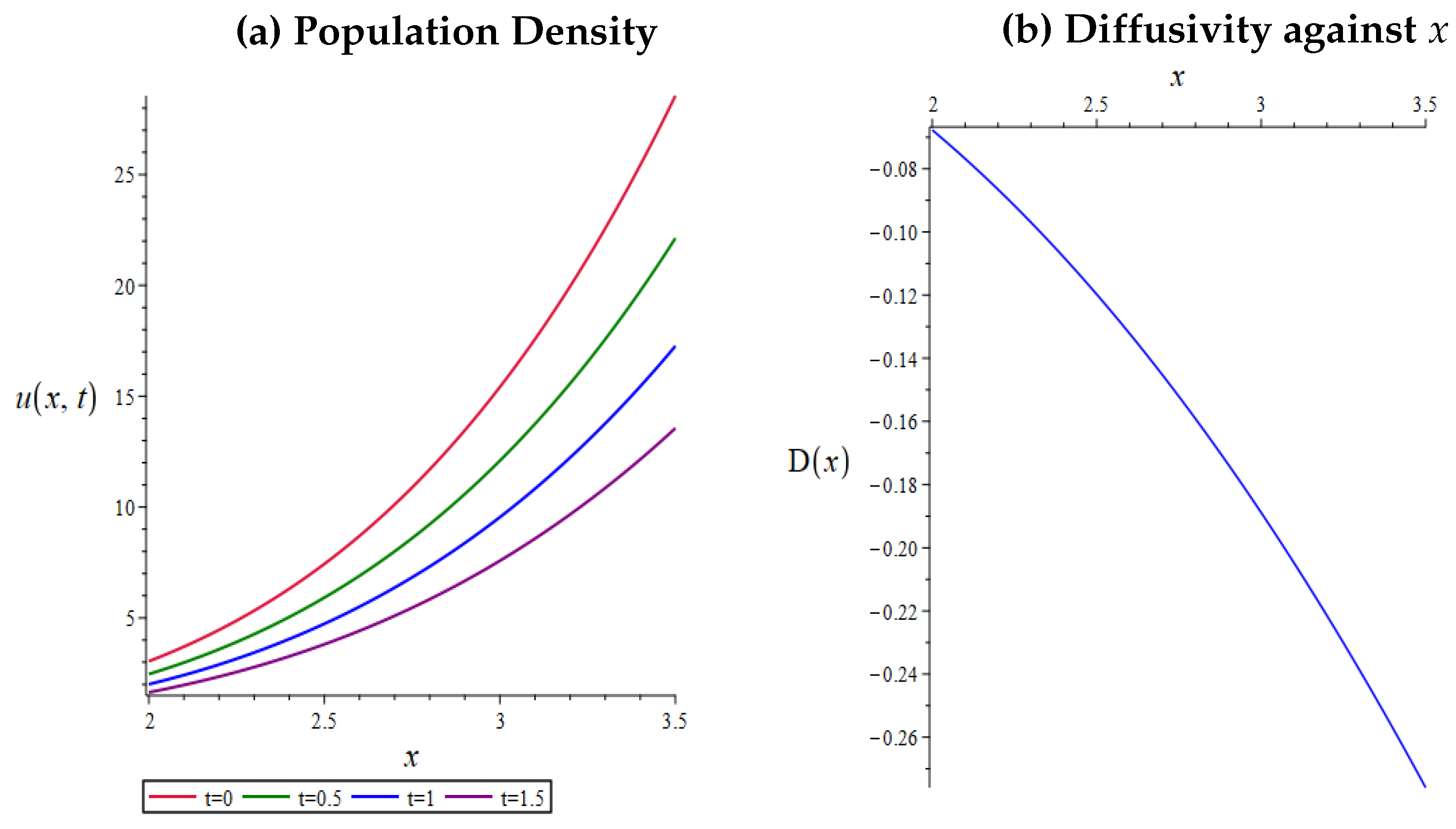
We observe the following for each $x\in \mathcal{H}$ for the given fixed values of t:

• the inhabitants aggregate to the boundary at $x=3.5$, since the population density increases at an increasing rate while the diffusivity is negative and decreases at a decreasing rate;
• the population density is bounded by $\mathcal{K}=e^6$;
• as t increases, the inhabitants continue to aggregate but are dying, since the density decreases.

The population eventually becomes extinct, since for all fixed x, $u(x,t)\to 0$ as $t\to \infty$. This reflects that the inhabitants of a population may aggregate to increase their survival chances against stronger predators, but this is only a temporary defence, since they can eventually be eliminated. We note that (16) blows up in global time when we have both $a_1<0$ and $a_5>0$. When $x>1$, (16) blows-up in finite time as $t\to {\displaystyle \frac{a_2^{+}}{a_1}}$ for particular values of $a_0$, $a_1$, $a_2$, $a_4$ and $a_5$. Blow-up phenomena may be better suited to applications in heat transfer.

4. Discussion and Outlook

This paper used the non-classical method with $T=0$ to search for non-Lie solutions to the class of reaction-diffusion equations (3). To find solutions to the single nonlinear determining equation, we imposed the ansatz $U=U(x,t,u)=F\left(x\right)G\left(t\right)H\left(u\right)$ and imposed additional constraints on the form of $H\left(u\right)$. As we could not solve the single determining equation completely, five cases were considered, each assuming a form of $H\left(u\right)$. Paths leading to $D^{\prime }\left(x\right)=0$, $G^{\prime }\left(t\right)=0$, $U=0$ or $Q\left(u\right)$ linear were not of interest and not pursued further. The case $H\left(u\right)=u>0$ led to two essentially non-classical symmetries. Each symmetry led to the construction of a solution. We proved our solutions are non-Lie and cannot be found by utilizing non-classical symmetries with $T\ne 0$.

One solution was used to discuss a potential model for describing population growth in biology with a Gompertz growth rate function. To the best of our knowledge, the first exact solution with a Gompertz-like growth rate function for nonlinear reaction-diffusion was constructed by Bradshaw-Hajek and Broadbridge [52]. We believe that our non-Lie solution (16) and our other non-Lie solution constitute the first non-Lie non-classical exact solutions associated with infinitesimal $T=0$ to (3) with a Gompertz growth rate function.

It is known that non-Lie solutions of (3) can be constructed using non-symmetry approaches. Such approaches include the direct method of Clarkson and Kruskal [19] used by Polyanin [18] and a direct method due to Polyanin [20]. These methods are all useful techniques for finding exact solutions. Here, we use our non-Lie solutions to demonstrate that the non-classical method with $T=0$ can lead to solutions that cannot be recovered under the assumptions of Polyanin’s [20] direct method. Polyanin’s method seeks solutions of (1) by imposing the ansatz

$$\int h\left(u\right)du=\xi \left(x\right)\omega \left(t\right)+\eta \left(x\right).$$

(21)

As the analysis is difficult, Polyanin separately imposes the two additional assumptions

$${\xi }^{\prime }\left(x\right)=0\mathrm{and}{\displaystyle \frac{d}{du}}\left({\displaystyle \frac{E\left(u\right)}{h\left(u\right)}}\right)=0.$$

(22)

The functions $h\left(u\right)$, $\xi \left(x\right)$, $\omega \left(t\right)$ and $\eta \left(x\right)$ are determined in the analysis and some solutions are found for (3). Our non-Lie solutions in Table 2 take the form

$$u=x^{A\left(t\right)}B\left(t\right),\mathrm{with}x>0,\mathrm{and}{A}^{\prime }\left(t\right)\ne 0.$$

(23)

Since our non-Lie solutions depend on x and t, we assume ${\omega }^{\prime }\left(t\right)$, $\xi \left(x\right)$, $A\left(t\right)$, $B\left(t\right)\ne 0$.

Case 1. Considering the first assumption in (22), we assume ${\xi }^{\prime }\left(x\right)=0$, so that WLOG we can set $\xi \left(x\right)=1$. Explicit solutions from (21) are given by

$$u=\mathsf{\Phi }\left(\omega \right(t)+\eta (x\left)\right),$$

where $\mathsf{\Phi }$ is the inverse of $\int h\left(u\right)du$. We impose ${\eta }^{\prime }\left(x\right)\ne 0$ as our non-Lie solutions depend on x and t. Equating the form of u directly above with (23) and their first-order differential consequences, respectively, we can show

$$\eta \left(x\right)=k_{1}ln(\pm (ln\left(x\right)+k_2))+k_3,\omega \left(t\right)=k_{1}ln(\pm A\left(t\right))+k_4,\mathrm{and}B\left(t\right)=k_5{e}^{k_{2}A\left(t\right)},$$

where $k_1$, $k_2$, $k_3$, $k_4$ and $k_5$ are constants. Note that the ± signs in $\eta \left(x\right)$ and $\omega \left(t\right)$, respectively, are unrelated. Taking $A\left(t\right)$ and $B\left(t\right)$ so that (23) represents our non-Lie solutions listed in Table 2, respectively, we can show $B\left(t\right)\ne k_5{e}^{k_{2}A\left(t\right)}$. Hence, (21) under the first assumption in (22) will not recover our non-Lie solutions.

Case 2. Considering the second assumption in (22) and equating (1) with (3), we can set $C\left(x\right)=E\left(u\right)=r\left(x\right)=1$ WLOG. Assuming ${\displaystyle \frac{d}{du}}\left({\displaystyle \frac{E\left(u\right)}{h\left(u\right)}}\right)=0$ with $E\left(u\right)=1$, we find $h\left(u\right)=const$. Solutions in the form (21) are given by

$$u=\xi \left(x\right)\omega \left(t\right)+\eta \left(x\right).$$

Equating the form of u directly above with (23), differentiating with respect to t once and x twice we can show

$${\omega }^{\prime }\left(t\right)\left(x^2{\xi }^{\prime \prime }\left(x\right)+x{\xi }^{\prime }\left(x\right)(1-2A\left(t\right))+{\left(A\left(t\right)\right)}^2\xi \left(x\right)\right)=0.$$

(24)

Since we assumed $A^{\prime }\left(t\right),{\omega }^{\prime }\left(t\right),\xi \left(x\right)\ne 0$, there is no solution to (24). Hence, (21) under the second assumption in (22) will not recover our non-Lie solutions. Recovering our non-Lie solutions using (21) may be possible under broader assumptions. We note that assuming ${\displaystyle \frac{d}{du}}\left({\displaystyle \frac{E\left(u\right)}{h\left(u\right)}}\right)=0$, (21) cannot find solutions of (3) in the form (23) that depend on x and t.

The construction of non-classical non-Lie solutions of (3) that cannot be found using non-classical symmetries with $T\ne 0$, nor with a direct method by Polyanin [20] under the assumptions in (22), constitutes the main result of the paper. We note that the ansatz $U=F\left(x\right)G\left(t\right)u$, despite its simplicity, appears to be special for (3). It may be useful for researchers who seek essentially non-classical symmetries with $T=0$ of other classes of one-dimensional reaction-diffusion equations where the reaction term depends on u alone, e.g., (1) with $r\left(x\right)=const$.

References

- Bakhvalov, P. ColESo: Collection of exact solutions for verification of numerical algorithms for simulation of compressible flows. Comput. Phys. Commun. 2023, 282, 108542. [Google Scholar] [CrossRef]
- Wilhelmsson, H. Explosive instabilities of reaction-diffusion equations. Phys. Rev. A 1987, 36, 965–966. [Google Scholar] [CrossRef]
- Bradshaw-Hajek, B.H.; Broadbridge, P. Analytic solutions for calcium ion fertilisation waves on the surface of eggs. Mathematical Medicine and Biology: A Journal of the IMA 2019, 36, 549–562. [Google Scholar] [CrossRef]
- Basarab-Horwath, P.; Lahno, V.; Zhdanov, R. The structure of Lie algebras and the classification problem for partial differential equations. Acta Appl. Math. 2001, 69, 43–94. [Google Scholar] [CrossRef]
- Vaneeva, O.O.; Johnpillai, A.G.; Popovych, R.O.; Sophocleous, C. Enhanced group analysis and conservation laws of variable coefficient reaction-diffusion equations with power nonlinearities. J. Math. Anal. Appl. 2007, 330, 1363–1386. [Google Scholar] [CrossRef]
- Vaneeva, O.O.; Popovych, R.O.; Sophocleous, C. Enhanced group analysis and exact solutions of variable coefficient semilinear diffusion equations with a power source. Acta Appl. Math. 2009, 106, 1–46. [Google Scholar] [CrossRef]
- Vaneeva, O.O.; Popovych, R.O.; Sophocleous, C. Extended group analysis of variable coefficient reaction-diffusion equations with exponential nonlinearities. J. Math. Anal. Appl. 2012, 396, 225–242. [Google Scholar] [CrossRef]
- Vaneeva, O. Group classification via mapping between classes: an example of semilinear reaction-diffusion equations with exponential nonlinearity. 2008, ArXiv: Nonlinear Sciences: Exactly Solvable and Integrable Systems 0811.2587. ArXiv.org e-Print archive. https://arxiv.org/abs/0811.2587.
- Vaneeva, O.O.; Popovych, R.O.; Sophocleous, C. Reduction operators of variable coefficient semilinear diffusion equations with a power source. 2009, ArXiv: Nonlinear Sciences: Exactly Solvable and Integrable Systems 0904.3424. ArXiv.org e-Print archive. https://arxiv.org/abs/0904.3424.
- Vaneeva, O.O.; Popovych, R.O.; Sophocleous, C. Reduction operators of variable coefficient semilinear diffusion equations with an exponential source. 2010, ArXiv: Nonlinear Sciences: Exactly Solvable and Integrable Systems 1010.2046. ArXiv.org e-Print archive. https://arxiv.org/abs/1010.2046.
- Broadbridge, P.; Bradshaw, B.H.; Fulford, G.R.; Aldis, G.K. Huxley and Fisher equations for gene propagation: an exact solution. ANZIAM J. 2002, 44, 11–20. [Google Scholar] [CrossRef]
- Le Roux, M.N.; Wilhelmsson, H. External boundary effects on simultaneous diffusion and reaction processes. Phys. Scr. 1989, 40, 674–681. [Google Scholar] [CrossRef]
- Moitsheki, R.J.; Bradshaw-Hajek, B.H. Symmetry analysis of a heat conduction model for heat transfer in a longitudinal rectangular fin of a heterogeneous material. Commun. Nonlinear Sci. Numer. Simul. 2013, 18, 2374–2387. [Google Scholar] [CrossRef]
- Braverman, E.; Braverman, L. Optimal harvesting of diffusive models in a nonhomogeneous environment. Nonlinear Anal. Theor. 2009, 71, e2173–e2181. [Google Scholar] [CrossRef]
- Bradshaw-Hajek, B.H.; Moitsheki, R.J. Symmetry solutions for reaction-diffusion equations with spatially dependent diffusivity. Appl. Math. Comput. 2015, 254, 30–38. [Google Scholar] [CrossRef]
- Bradshaw-Hajek, B.H. Nonclassical symmetry solutions for non-autonomous reaction-diffusion equations. Symmetry 2019, 11, 208. [Google Scholar] [CrossRef]
- Polyanin, A.D.; Zhurov, A.I. Separation of Variables and Exact Solutions to Nonlinear PDEs, 1st ed.; CRC Press: Boca Raton, FL, USA, 2022; ISBN 978-0-367-48689-1. [Google Scholar]
- Polyanin, A.D. Functional separable solutions of nonlinear reaction–diffusion equations with variable coefficients. Appl. Math. Comput. 2019, 347, 282–292. [Google Scholar] [CrossRef]
- Clarkson, P.A.; Kruskal, M.D. New similarity reductions of the Boussinesq equation. J. Math. Phys. 1989, 30, 2201–2213. [Google Scholar] [CrossRef]
- Polyanin, A.D. Construction of exact solutions in implicit form for PDEs: new functional separable solutions of non-linear reaction–diffusion equations with variable coefficients. Int. J. Non-Linear Mech. 2019, 111, 95–105. [Google Scholar] [CrossRef]
- Rocha, E.M.; Rodrigues, M.M. Exact and Approximate Solutions of Reaction-Diffusion-Convection Equations. Conference on Boundary Value Problems: Mathematical Models in Engineering, Biology and Medicine;, 2008; Vol. 1142, pp. 304–313. [CrossRef]
- Lie, S. Über die integration durch bestimmte integrale von einer classe linearer partieller differentialgleichungen. Archiv der Mathematik 1881, 6, 328–368. (in German). [Google Scholar]
- Lie, S. Allgemeine untersuchungen über differentialgleichungen, die eine continuirliche, endliche gruppe gestatten. Mathematische Annalen 1885, 25, 71–151. (in German). [Google Scholar] [CrossRef]
- Arrigo, D. Symmetry Analysis of Differential Equations, 1st ed.; John Wiley & Sons Inc: Hoboken, NJ, USA, 2015; ISBN 978-1118721407. [Google Scholar]
- Sherring, J. Dimsym Users Manual. Melbourne, Victoria, Australia, 1993.
- Hearn, T. REDUCE; A Portable General-Purpose Computer Algebra System, SourceForge, 2022. Available online at https://sourceforge.net/projects/reduce-algebra/.
- Cheviakov, A.F. GeM software package for computation of symmetries and conservation laws of differential equations. Comput. Phys. Commun. 2007, 176, 48–61. [Google Scholar] [CrossRef]
- Maple (2021), Maplesoft, a Division of Waterloo Maple Incorporated; Waterloo, Ontario, 2021.
- Olver, P.J. Applications of Lie Groups to Differential Equations, 2nd ed.; Springer: New York, NY, USA, 1993; ISBN 9781461243502. [Google Scholar]
- Ovsiannikov, L.V. Group Analysis of Differential Equations: Ames, W.F. Eds.; Academic Press Incorporated: New York, NY, USA, 1982; ISBN 978-0-12-531680-4. [Google Scholar]
- Bluman, G.W. Construction of Solutions to Partial Differential Equations by the Use of Transformation Groups. Ph.D. Dissertation, California Institute of Technology, Pasadena, CA, USA, November 14 1967. [Google Scholar]
- Bluman, G.W.; Cole, J.D. The general similarity solution of the heat equation. J. Math. Mech. 1969, 18, 1025–1042. [Google Scholar]
- Fushchych, W.I. On symmetry and particular solutions of some multidimensional physics equations. Algebraic-Theoretical Methods in Mathematical Physics Problems, Institute of Mathematics of the National Academy of Sciences of Ukraine.
- Fushchych, W.I.; Serov, M.I.; Chopyk, V.I. Conditional invariance and nonlinear heat equations. Proceedings of the Academy of Sciences of Ukraine 1988, 9, 17–21. [Google Scholar]
- Popovych, R. No-go theorem on reduction operators of linear second-order parabolic equations. Proceedings of the Institute of Mathematics of the National Academy of Sciences of Ukraine 2006, 3, 231–238. [Google Scholar]
- Bluman, G.W.; Anco, S.C. Symmetry and Integration Methods for Differential Equations, 2nd ed.; Springer: New York, NY, USA, 2002; ISBN 978-0-387-98654-8. [Google Scholar]
- Burde, G.I. Partially nonclassical method and conformal invariance in the context of the Lie group method. Symmetry 2024, 16, 875. [Google Scholar] [CrossRef]
- Arrigo, D.J.; Goard, J.M.; Broadbridge, P. Nonclassical solutions are non-existent for the heat equation and rare for nonlinear diffusion. J. Math. Anal. Appl. 1996, 202, 259–279. [Google Scholar] [CrossRef]
- Cherniha, R.M. New non-Lie ansätze and exact solutions of nonlinear reaction-diffusion-convection equations. J. Phys. A Math. Gen. 1998, 31, 8179–8198. [Google Scholar] [CrossRef]
- Cherniha, R.; Serov, M.; Pliukhin, O. Lie and Q-Conditional symmetries of reaction-diffusion-convection equations with exponential nonlinearities and their application for finding exact solutions. Symmetry 2018, 10, 123. [Google Scholar] [CrossRef]
- Clarkson, P.A.; Mansfield, E.L. Symmetry reductions and exact solutions of a class of nonlinear heat equations. Phys. D 1994, 70, 250–288. [Google Scholar] [CrossRef]
- Arrigo, D.J.; Hill, J.M. Nonclassical symmetries for nonlinear diffusion and absorption. Stud. Appl. Math. 1995, 94, 21–39. [Google Scholar] [CrossRef]
- Arrigo, D.J.; Hill, J.M.; Broadbridge, P. Nonclassical symmetry reductions of the linear diffusion equation with a nonlinear source. IMA J. Appl. Math. 1994, 52, 1–24. [Google Scholar] [CrossRef]
- Ibragimov, N.H. CRC Handbook of Lie Group Analysis of Differential Equations, Volume 1: Symmetries, Exact Solutions, and Conservation Laws; CRC Press: Boca Raton, FL, USA, 1993. ISBN 978100341 9808.
- Zhdanov, R.Z.; Lahno, V.I. Conditional symmetry of a porous medium equation. Phys. D 1998, 122, 178–186. [Google Scholar] [CrossRef]
- Bradshaw-Hajek, B.H.; Edwards, M.P.; Broadbridge, P.; Williams, G.H. Nonclassical symmetry solutions for reaction-diffusion equations with explicit spatial dependence. Nonlinear Anal. 2007, 67, 2541–2552. [Google Scholar] [CrossRef]
- Lewis, M.A.; Petrovskii, S.V.; Potts, J.R. The Mathematics Behind Biological Invasions, 1st ed.; Springer Nature: Berlin, Germany, 2016; ISBN 978-3-319-32042-7. [Google Scholar]
- Fick, A. Ueber diffusion. Ann. Phys. 1855, 170, 59–86. [Google Scholar] [CrossRef]
- Grünbaum, D.; Okubo, A. , Germany, 1994; Vol. 100, pp. 296–325. ISBN 978-3-642-50124-1.Aggregations. In Frontiers in Mathematical Biology. Lecture Notes in Biomathematics; Springer: Heidelberg, Germany, 1994; ISBN 978-3-642-50124-1. [Google Scholar]
- Muskox: Circle Defense. Available online: https://home.nps.gov/gaar/learn/nature/muskox-circle-defense.htm#:~:text=When%20they%20see%20danger%20approaching,phalanx%20of%20heads%20and%20horns. (accessed on 2 October 2024).
- Gompertz, B. On the nature of the function expressive of the law of human mortality, and on a new mode of determining the value of life contingencies. Phil. Trans. R. Soc. 1825, 115, 513–583. [Google Scholar] [CrossRef]
- Bradshaw-Hajek, B.H.; Broadbridge, P. An analytic solution for a Gompertz-like reaction-diffusion model for tumour growth. Adv. Stud. Pure Math. 2020, 85, 127–136. [Google Scholar] [CrossRef]