Machine Learning Method for Approximate Solutions for Reaction-Diffusion Equations with Multivalued Interaction Functions

1. Introduction

In this paper we establish machine learning methods for approximate solutions of classes of reaction-diffusion equations with multivalued interaction functions allowing for non-unique solutions of the Cauchy problem. The relevance of this problem is primarily due to the lack of methods for finding all solutions for such mathematical objects. Therefore, there is an expectation that another approximate method will provide us with yet another solution for these problems. In addition, methods for approximate solutions of nonlinear systems with partial derivatives without uniqueness are mostly theoretical and are used primarily in qualitative research [1,2]. The availability of computational power for parallel computations and the creation of open-source software libraries such as PyTorch [3] have stimulated a new wave of development in IT and artificial intelligence methods. Sample-based methods for approximate solutions of such problems were first proposed in [4]. To date, such systems with smooth nonlinearities have been qualitatively and numerically studied. There is a need to develop a methodology for approximating generalized solutions of nonlinear differential-operator systems without uniqueness using recurrent neural networks, sample-based methods, and variations of the Monte Carlo method.

Let $T,\nu >0,$ and $u_0:{\mathbb{R}}^2\to \mathbb{R}$ be a sufficiently smooth function. We consider the problem:

$${\displaystyle \frac{\partial u}{\partial t}}(x,t)\in \nu {\nabla }^{2}u(x,t)-f\left(u(x,t)\right),(x,t)\in {\mathbb{R}}^2\times [0,T],$$

(1)

with initial conditions:

$$u(x,0)=u_0\left(x\right),x\in {\mathbb{R}}^2,$$

(2)

where $f:\mathbb{R}\to \mathbb{R}$ is a function satisfying the condition of at most linear growth:

$$\exists C>0:\left|f\right(s\left)\right|\le C(1+|s\left|\right)\mathrm{for}\mathrm{each}s\in \mathbb{R}.$$

We note that such nonlinearities appear in impulse feedback control problems, etc. [5,6,7,8,9]. Moreover, the global attractor for solutions of Problem 1 may be a nontrivial set in the general case and can have arbitrarily large fractal dimension. The convergence rate of solutions to the attractor may not be exponential; see [10,11,12,13,14] and references therein.

For a fixed $u_0\in C_0^{\infty }\left({\mathbb{R}}^2\right)$ let $\mathsf{\Omega }\subset {\mathbb{R}}^2$ be a bounded domain with sufficiently smooth boundary and $\mathrm{supp}{u}_0\subset \mathsf{\Omega }.$ According to [1] (see the book and references therein), there exists a weak solution $u=u(x,t)\in L^2(0,T;H_0^1\left(\mathsf{\Omega }\right))$ with ${\displaystyle \frac{\partial u}{\partial t}}\in L^2(0,T;H^{-1}\left(\mathsf{\Omega }\right)),$ of Problem (1)–(2) in the following sense:

$$-{\int }_0^T{\int }_{\mathsf{\Omega }}u(x,t)v\left(x\right){\eta }_t\left(t\right)dxdt+\nu {\int }_0^T{\int }_{\mathsf{\Omega }}(\nabla u(x,t)·\nabla v\left(x\right)+d(x,t)v\left(x\right))\eta \left(t\right)dt=0,$$

(3)

for all $v\in C_0^{\infty }\left(\mathsf{\Omega }\right),\eta \in C_0^{\infty }(0,T),$ where $d:\mathbb{R}\times [0,T]\to \mathbb{R}$ be a measurable function such that

$$d(x,t)\in f\left(u(x,t)\right)fora.e.(x,t)\in {\mathbb{R}}^2\times (0,T).$$

(4)

Such inclusions with multivalued nonlinearities appear in problems of climatology (Budyko-Sellers Model), chemical kinetics (Belousov-Zhabotinsky equations), biology (Lotka–Volterra systems with diffusion), quantum mechanics (FitzHugh–Nagumo system), engineering and medicine (several syntheses and impulse control problems); see [1,2] and references therein.

The main goal of this paper is to develop an algorithm for approximation of solutions for classes of reaction-diffusion equations with multivalued interaction functions allowing for non-unique solutions of the Cauchy problem (1)–(2) via the so-called physics-informed neural networks (PINNs); [15,16,17] and references therein.

2. Methodology of Approximate Solutions for Reaction-Diffusion Equations with Multivalued Interaction Functions

Fix an arbitrary $T>0,$ and a sufficiently smooth function $u_0:{\mathbb{R}}^2\to \mathbb{R}.$ We approximate the function f by the following Lipschitz functions satisfying the condition of at most linear growth (Pasch-Hausdorff envelopes):

$$f_k\left(x\right):=\underset{x^{\prime }\in \mathbb{R}}{inf}\left\{f\left(x^{\prime }\right)+k|x-x^{\prime }|\right\},x\in \mathbb{R};$$

(5)

see [18] and references therein. For a fixed $k=1,2,\dots ,$ consider the problem:

$${\displaystyle \frac{\partial u_k}{\partial t}}(x,t)=\nu {\nabla }^2{u}_k(x,t)-f_k\left(u_k(x,t)\right),(x,t)\in {\mathbb{R}}^2\times [0,T],$$

(6)

with initial conditions:

$$u_k(x,0)=u_0\left(x\right),x\in {\mathbb{R}}^2.$$

(7)

According to [2] and references therein, for each $k=1,2,\dots$ Problem (6)–(7) has an unique solution $u_k\in C^{2,1}({\mathbb{R}}^2\times [0,T]).$ Moreover, [19] implies that each convergent subsequence ${\left\{u_{k_l}\right\}}_{l=1,2,\dots }\subset {\left\{u_k\right\}}_{k=1,2,\dots }$ of corresponding solutions to Problem (6)–(7) weakly converges to a solution u of Problem (1)–(2) in the space

$$W:=\{z\in L^2(0,T;H_0^1\left(\mathsf{\Omega }\right)):{\displaystyle \frac{\partial z}{\partial t}}\in L^2(0,T;H^{-1}\left(\mathsf{\Omega }\right))\}$$

(8)

endowed with the standard graph norm, where $\mathsf{\Omega }\subset {\mathbb{R}}^2$ is a bounded domain with sufficiently smooth boundary and $\mathrm{supp}{u}_0\subset \mathsf{\Omega }.$

Further, to simplify the conclusions we consider as f the following function:

$$f\left(s\right):=\left\{\begin{array}{cc}\left\{0\right\},& s<0;\hfill \\ \left[0,1\right],& s=0;\hfill \\ \left\{1\right\},& s>0.\hfill \end{array}\right.$$

(9)

We approximate it by the following Lipschitz functions:

$$f_k\left(s\right):=\left\{\begin{array}{cc}0,& s<0;\hfill \\ ks,& s\in [0,{\displaystyle \frac{1}{k}});\hfill \\ 1,& s\ge {\displaystyle \frac{1}{k}},\hfill \end{array}\right.k=1,2,\dots .$$

(10)

Thus, the first step of the algorithm is to replace the function f in Problem (1)–(2) with $f_k$ considering Problem (6)–(7) for sufficiently large $k.$

Let us now consider Problem (6)–(7) for sufficiently large $k.$ Theorem 16.1.1 from [15] allows us to reformulate Problem (6)–(7) as an infinite dimensional stochastic optimization problem over a certain function space. More exactly, let $\mathtt{t}\in C\left(\right[0,T];(0,\infty \left)\right)$, $\xi \in C({\mathbb{R}}^2;(0,\infty )),$ let $(\mathsf{\Omega },\mathcal{F},\mathbb{P})$ be a probability space, let $\mathcal{T}:\mathsf{\Omega }\to [0,T]$ and $\mathcal{X}:\mathsf{\Omega }\to {\mathbb{R}}^2$ be independent random variables. Assume for all $A\in \mathcal{B}\left(\right[0,T\left]\right)$, $B\in \mathcal{B}\left({\mathbb{R}}^2\right)$ that

$$\mathbb{P}(\mathcal{T}\in A)={\int }_A\mathtt{t}\left(t\right)dt\mathrm{and}\mathbb{P}(\mathcal{X}\in B)={\int }_B\xi \left(x\right)dx.$$

Note that $f_k:\mathbb{R}\to \mathbb{R}$ be Lipschitz continuous, and let ${\mathcal{L}}_k:C^{2,1}({\mathbb{R}}^2\times [0,T],\mathbb{R})\to [0,\infty ]$ satisfy for all $v={\left(v(x,t)\right)}_{(x,t)\in {\mathbb{R}}^2\times [0,T]}\in C^{2,1}({\mathbb{R}}^2\times [0,T])$ that

$${\mathcal{L}}_k\left(v\right)=\mathbb{E}\left[{\left|v(\mathcal{X},0)-u_0\left(\mathcal{X}\right)\right|}^2+{\left|{\displaystyle \frac{\partial v}{\partial t}}(\mathcal{X},\mathcal{T})-\nu {\nabla }^{2}v(\mathcal{X},\mathcal{T})+f_k\left(v(\mathcal{X},\mathcal{T})\right)\right|}^2\right].$$

Theorem 16.1.1 from [15] implies that the following two statements are equivalent:

• It holds that ${\mathcal{L}}_k\left(u_k\right)={inf}_{v\in C^{2,1}({\mathbb{R}}^2\times [0,T])}{\mathcal{L}}_k\left(v\right)$.
• It holds $u_k\in C^{2,1}({\mathbb{R}}^2\times [0,T])$ is the solution of Problem (6)–(7).

Thus, the second step of the algorithm is to reduce the regularized Problem (6)–(7) to the infinite dimensional stochastic optimization problem in $C^{2,1}({\mathbb{R}}^2\times [0,T]):$

$$\left\{\begin{array}{c}{\mathcal{L}}_k\left(v\right)\to min,\hfill \\ v\in C^{2,1}({\mathbb{R}}^2\times [0,T]).\hfill \end{array}\right.$$

(11)

However, due to its infinite dimensionality, the optimization problem (11) is not yet suitable for numerical computations. Therefore, we apply the third step, the so-called Deep Galerkin Method (DGM) [20], that is, we transform this infinite dimensional stochastic optimization problem into a finite dimensional one by incorporating artificial neural networks (ANNs); see [15,20] and references therein. Let $a:\mathbb{R}\to \mathbb{R}$ be differentiable, let $h\in \mathbb{N},l_1,l_2,...,l_h,\mathfrak{d}\in \mathbb{N}$ satisfy $\mathfrak{d}=4l_1+\left[{\sum }_{k=2}^h{l}_k(l_{k-1}+1)\right]+l_h+1$, and let ${\mathcal{L}}_{k,h}:{\mathbb{R}}^{\mathfrak{d}}\to [0,\infty )$ satisfy for all $\theta \in {\mathbb{R}}^{\mathfrak{d}}$ that

$$\begin{array}{cc}\hfill {\mathcal{L}}_{k,h}\left(\theta \right)& ={\mathcal{L}}_k\left({\mathcal{N}}_{{\mathfrak{M}}_{a,l_1},{\mathfrak{M}}_{a,l_2},...,{\mathfrak{M}}_{a,l_h},{\mathrm{id}}_{\mathbb{R}}}^{\theta ,3}\right)\hfill \\ \hfill & =\mathbb{E}\left[{\left|{\mathcal{N}}_{{\mathfrak{M}}_{a,l_1},\dots ,{\mathfrak{M}}_{a,l_h},{\mathrm{id}}_{\mathbb{R}}}^{\theta ,3}(\mathcal{X},0)-u_0\left(\mathcal{X}\right)\right|}^2\right.\hfill \\ \hfill & +\left|{\displaystyle \frac{\partial {\mathcal{N}}_{{\mathfrak{M}}_{a,l_1},\dots ,{\mathfrak{M}}_{a,l_h},{\mathrm{id}}_{\mathbb{R}}}^{\theta ,3}}{\partial t}}(\mathcal{X},\mathcal{T})-\nu {\nabla }^2{\mathcal{N}}_{{\mathfrak{M}}_{a,l_1},\dots ,{\mathfrak{M}}_{a,l_h},{\mathrm{id}}_{\mathbb{R}}}^{\theta ,3}(\mathcal{X},\mathcal{T})\right.\hfill \\ \hfill & \left.{\left.+f_k\left({\mathcal{N}}_{{\mathfrak{M}}_{a,l_1},\dots ,{\mathfrak{M}}_{a,l_h},{\mathrm{id}}_{\mathbb{R}}}^{\theta ,3}(\mathcal{X},\mathcal{T})\right)\right|}^2\right],\hfill \end{array}$$

(12)

where ${\mathfrak{M}}_{\psi ,d}$ is the d-dimensional version of a function $\psi ,$ that is,

$${\mathfrak{M}}_{\psi ,d}:{\mathbb{R}}^d\to {\mathbb{R}}^d$$

is the function which satisfies for all $x={\left(x_k\right)}_{k\in \{1,2,\dots ,d\}}\in {\mathbb{R}}^d$, $y={\left(y_k\right)}_{k\in \{1,2,\dots ,d\}}\in {\mathbb{R}}^d$ with $\forall k\in \{1,2,\dots ,d\}:$$y_k=\psi \left(x_k\right)$ that

$${\mathfrak{M}}_{\psi ,d}\left(x\right)=y;$$

for each $\mathfrak{d},L\in \mathbb{N},l_0,l_1,...,l_L\in \mathbb{N},\theta \in {\mathbb{R}}^{\mathfrak{d}}$ satisfying $\mathfrak{d}\ge {\sum }_{k=1}^L{l}_k(l_{k-1}+1),$ and for a function ${\mathsf{\Psi }}_k:{\mathbb{R}}^{l_k}\to {\mathbb{R}}^{l_k},$ $k\in \{1,2,...,L\},$ we denote by ${\mathcal{N}}_{{\mathsf{\Psi }}_1,{\mathsf{\Psi }}_2,...,{\mathsf{\Psi }}_L}^{\theta ,l_0}:{\mathbb{R}}^{l_0}\to {\mathbb{R}}^{l_L}$ the realization function of the fully-connected feedforward artificial neural network associated to $\theta$ with $L+1$ layers with dimensions $(l_0,l_1,...,l_L)$ and activation functions $({\mathsf{\Psi }}_1,{\mathsf{\Psi }}_2,...{\mathsf{\Psi }}_L),$ defined as:

$$\begin{array}{c}\hfill {\mathcal{N}}_{{\mathsf{\Psi }}_1,{\mathsf{\Psi }}_2,...,{\mathsf{\Psi }}_L}^{\theta ,l_0}\left(x\right)=({\mathsf{\Psi }}_L\circ {\mathcal{A}}_{l_L,l_{L-1}}^{\theta ,{\sum }_{k=1}^{L-1}{l}_k(l_{k-1}+1)}\circ {\mathsf{\Psi }}_{L-1}\circ {\mathcal{A}}_{l_{L-1},l_{L-2}}^{\theta ,{\sum }_{k=1}^{L-2}{l}_k(l_{k-1}+1)}\circ ...\\ \hfill ...\circ {\mathsf{\Psi }}_2\circ {\mathcal{A}}_{l_2,l_1}^{\theta ,l_1(l_0+1)}\circ {\mathsf{\Psi }}_1\circ {\mathcal{A}}_{l_1,l_0}^{\theta ,0})\left(x\right),\end{array}$$

for all $x\in {\mathbb{R}}^{l_0};$ and for each $\mathtt{d},m,n\in \mathbb{N},$$s\in {\mathbb{N}}_0:=\mathbb{N}\cup \left\{0\right\},$$\theta =({\theta }_1,{\theta }_2,\dots ,{\theta }_{\mathtt{d}})\in {\mathbb{R}}^{\mathtt{d}}$ satisfying $\mathtt{d}\ge s+mn+m,$ the affine function ${\mathcal{A}}_{s,m,n}^{\theta }$ from ${\mathbb{R}}^n$ to ${\mathbb{R}}^m$ associated to $(\theta ,s),$ is defined as

$${\mathcal{A}}_{s,m,n}^{\theta }\left(x\right)=\left(\begin{array}{cccc}{\theta }_{s+1}& {\theta }_{s+2}& \cdots & {\theta }_{s+n}\\ {\theta }_{s+n+1}& {\theta }_{s+n+2}& \cdots & {\theta }_{s+2n}\\ {\theta }_{s+2n+1}& {\theta }_{s+2n+2}& \cdots & {\theta }_{s+3n}\\ ⋮& ⋮& \ddots & ⋮\\ {\theta }_{s+(m-1)n+1}& {\theta }_{s+(m-1)n+2}& \cdots & {\theta }_{s+mn}\end{array}\right)\left(\begin{array}{c}{x}_1\\ x_2\\ ⋮\\ x_n\end{array}\right)+\left(\begin{array}{c}{\theta }_{s+mn+1}\\ {\theta }_{s+mn+2}\\ ⋮\\ {\theta }_{s+mn+m}\end{array}\right)$$

for all $x=(x_1,x_2,\dots ,x_n)\in {\mathbb{R}}^n.$

The final step in the derivation involves approximating the minimizer of ${\mathcal{L}}_{k,h}$ using stochastic gradient descent optimization methods [15]. Let $\xi \in {\mathbb{R}}^{\mathfrak{d}}$, $J\in \mathbb{N}$, ${\left({\gamma }_n\right)}_{n\in \mathbb{N}}\subseteq [0,\infty ),$ for each $n\in \mathbb{N},$$j\in \{1,2,...,J\}$ let $\mathfrak{T}:\mathsf{\Omega }\to [0,T]$ and ${\mathfrak{X}}_{n,j}:\mathsf{\Omega }\to {\mathbb{R}}^2$ be random variables. Let for each $n\in \mathbb{N},$$j\in \{1,2,...,J\},$$A\in \mathcal{B}\left(\right[0,T\left]\right),$$B\in \mathcal{B}\left({\mathbb{R}}^2\right)$

$$\mathbb{P}(\mathcal{T}\in A)=\mathbb{P}({\mathfrak{T}}_{n,j}\in A)\mathrm{and}\mathbb{P}(\mathcal{X}\in B)=\mathbb{P}({\mathfrak{X}}_{n,j}\in B).$$

(13)

Let ${\ell }_{k,h}:{\mathbb{R}}^{\mathfrak{d}}\times {\mathbb{R}}^2\times [0,T]\to \mathbb{R}$ is defined as

$$\begin{array}{cc}\hfill {\ell }_{k,h}(\theta ,x,t)=& {\left|{\mathcal{N}}_{{\mathfrak{M}}_{a,l_1},{\mathfrak{M}}_{a,l_2},\dots ,{\mathfrak{M}}_{a,l_h},{\mathrm{id}}_{\mathbb{R}}}^{\theta ,3}(x,0)-u_0\left(x\right)\right|}^2\hfill \\ \hfill & +\left|{\displaystyle \frac{\partial {\mathcal{N}}_{{\mathfrak{M}}_{a,l_1},{\mathfrak{M}}_{a,l_2},\dots ,{\mathfrak{M}}_{a,l_h},{\mathrm{id}}_{\mathbb{R}}}^{\theta ,3}}{\partial t}}(x,t)-\nu {\nabla }^2{\mathcal{N}}_{{\mathfrak{M}}_{a,l_1},{\mathfrak{M}}_{a,l_2},\dots ,{\mathfrak{M}}_{a,l_h},{\mathrm{id}}_{\mathbb{R}}}^{\theta ,3}(x,t)\right.\hfill \\ \hfill & {\left.+f_k\left({\mathcal{N}}_{{\mathfrak{M}}_{a,l_1},{\mathfrak{M}}_{a,l_2},\dots ,{\mathfrak{M}}_{a,l_h},{\mathrm{id}}_{\mathbb{R}}}^{\theta ,3}(x,t)\right)\right|}^2,\hfill \end{array}$$

(14)

for each $\theta \in {\mathbb{R}}^{\mathfrak{d}},$$x\in {\mathbb{R}}^2,$$t\in [0,T],$ and let $\mathsf{\Theta }={\left({\mathsf{\Theta }}_n\right)}_{n\in {\mathbb{N}}_0}:{\mathbb{N}}_0\times \mathsf{\Omega }\to {\mathbb{R}}^{\mathfrak{d}}$ satisfy for all $n\in \mathbb{N}$ that

$${\mathsf{\Theta }}_0=\xi \mathrm{and}{\mathsf{\Theta }}_n={\mathsf{\Theta }}_{n-1}-{\gamma }_n\left[{\displaystyle \frac{1}{J}}\sum _{j=1}^J\left({\nabla }_{\theta }{\ell }_{k,h}\right)({\mathsf{\Theta }}_{n-1},{\mathfrak{T}}_{n,j},{\mathfrak{X}}_{n,j})\right].$$

(15)

Ultimately, for sufficiently large $k,h,n\in \mathbb{N},$ the realization ${\mathcal{N}}_{{\mathfrak{M}}_{a,l_1},{\mathfrak{M}}_{a,l_2},\dots ,{\mathfrak{M}}_{a,l_h},{\mathrm{id}}_{\mathbb{R}}}^{{\mathsf{\Theta }}_n,3}$ is chosen as an approximation:

$${\mathcal{N}}_{{\mathfrak{M}}_{a,l_1},{\mathfrak{M}}_{a,l_2},\dots ,{\mathfrak{M}}_{a,l_h},{\mathrm{id}}_{\mathbb{R}}}^{{\mathsf{\Theta }}_n,3}\approx u$$

of the unknown solution u of (1)–(2) in the space W defined in (8).

So, the following theorem is justified.

Theorem 1. 

Let $T>0,$ and $u_0\in C_0^{\infty }\left({\mathbb{R}}^2\right).$ Then the sequence of ${\left\{{\mathcal{N}}_{{\mathfrak{M}}_{a,l_1},{\mathfrak{M}}_{a,l_2},\dots ,{\mathfrak{M}}_{a,l_h},{\mathrm{id}}_{\mathbb{R}}}^{{\mathsf{\Theta }}_n,3}\right\}}_{k,h,n}$ defined in (14)–(15) has an accumulation point in the weak topology of W defined in (8). Moreover, each partial limit of the sequence in hands is weakly converges in W to the solution of Problem (1)–(2) in the sense of (3)–(4).

Proof. 

According to Steps 1–4 above, to derive PINNs, we approximate u in the space W defined in (8) by a deep ANN ${\mathcal{N}}_{\theta }:{\mathbb{R}}^2\times [0,T]\to \mathbb{R}$ with parameters $\theta \in {\mathbb{R}}^{\mathfrak{d}}$ and minimize the empirical risk associated to ${\mathcal{L}}_k\left(v\right)$ over the parameter space ${\mathbb{R}}^{\mathfrak{d}}$. More precisely, we approximate the solution u of (1)–(2) by ${\mathcal{N}}_{{\theta }^{\ast }}$ where

$${\theta }^{\ast }\in arg\underset{\theta \in {\mathbb{R}}^{\mathfrak{d}}}{min}{\displaystyle \frac{1}{n}}\sum _{i=1}^n\left[{\left|{\mathcal{N}}_{\theta }(X_i,0)-u_0\left(X_i\right)\right|}^2+{\left|{\displaystyle \frac{\partial {\mathcal{N}}_{\theta }}{\partial t}}(X_i,T_i)-\nu {\nabla }^2{\mathcal{N}}_{\theta }(X_i,T_i)+f_k\left({\mathcal{N}}_{\theta }(X_i,T_i)\right)\right|}^2\right]$$

for a suitable choice of training data ${\left\{(X_i,T_i)\right\}}_{i=1}^n$. Here $n\in \mathbb{N}$ denotes the number of training samples and the pairs $(X_i,T_i)$, $i\in \{1,2,\dots ,n\},$ denote the realizations of the random variables X and T.

Analogously, to derive DGMs, we approximate u by a deep Galerkin method (DGM) ${\mathcal{G}}_{\theta }:{\mathbb{R}}^2\times [0,T]\to \mathbb{R}$ with parameters $\theta \in {\mathbb{R}}^{\mathfrak{d}}$ and minimize the empirical risk associated to ${\mathcal{L}}_{k,h}\left(v\right)$ over the parameter space ${\mathbb{R}}^{\mathfrak{d}}.$ More precisely, we approximate the solution u of (1)–(2) by ${\mathcal{G}}_{{\theta }^{\ast }},$ where

$${\theta }^{\ast }\in arg\underset{\theta \in {\mathbb{R}}^{\mathfrak{d}}}{min}{\displaystyle \frac{1}{n}}\sum _{i=1}^n\left[{\left|{\mathcal{G}}_{\theta }(X_i,0)-u_0\left(X_i\right)\right|}^2+{\left|{\displaystyle \frac{\partial {\mathcal{G}}_{\theta }}{\partial t}}(X_i,T_i)-\nu {\nabla }^2{\mathcal{G}}_{\theta }(X_i,T_i)+f_k\left({\mathcal{G}}_{\theta }(X_i,T_i)\right)\right|}^2\right]$$

for a suitable choice (please, see the third (final) step above for details) of training data ${\left\{(X_i,T_i)\right\}}_{i=1}^n$. Here $n\in \mathbb{N}$ denotes the number of training samples and the pairs $(X_i,T_i)$, $i\in \{1,2,\dots ,n\},$ denote the realizations of the random variables X and T.    □

The empirical risk minimization problems for PINNs and DGMs are typically solved using SGD or variants thereof, such as Adam [15]. The gradients of the empirical risk with respect to the parameters $\theta$ can be computed efficiently using automatic differentiation, which is commonly available in deep learning frameworks such as TensorFlow and PyTorch. We provide implementation details and numerical simulations for PINNs and DGMs in the next section.

3. Numerical Implementation

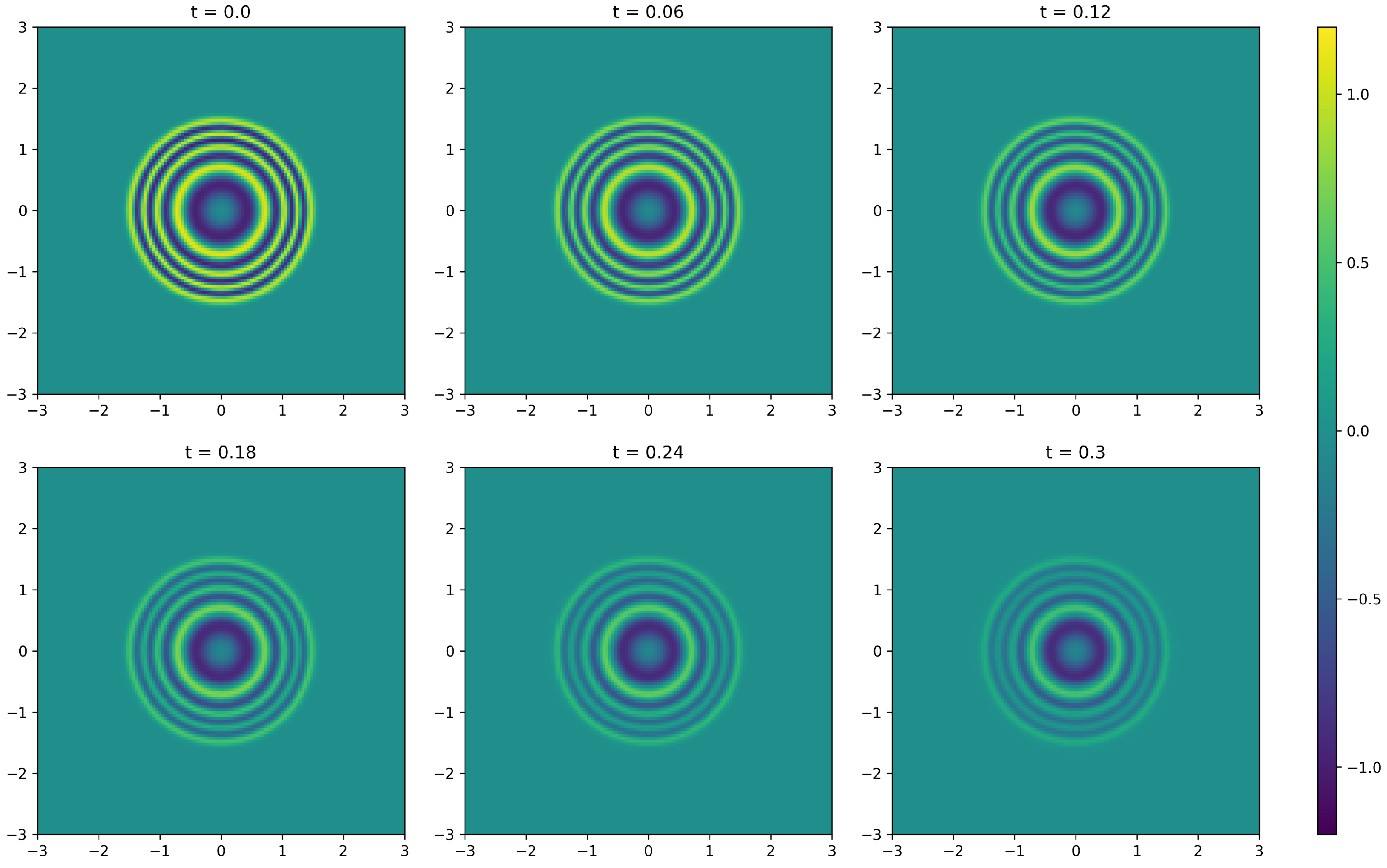
Let us present a straightforward implementation of the method as detailed in the previous Section for approximating a solution $u\in W$ of Problem (1)–(2) with $\nu =0.005,$ and the initial condition $u_0\left(x\right):=\psi (x_1^2+x_2^2),$ where

$$\psi \left(s\right):=\left\{\begin{array}{cc}sin(8\pi exp\left(1-{\displaystyle \frac{3}{3-s}}\right),\hfill & s\in [0,3);\hfill \\ 0,\hfill & \mathrm{otherwise},\hfill \end{array}\right.$$

(16)

$(x_1,x_2)\in {\mathbb{R}}^2.$ Let $k=0.01.$ This implementation follows the original proposal by [16], where $20.000$ realizations of the random variable $(\mathcal{X},\mathcal{T})$ are first chosen. Here, $\mathcal{T}$ is uniformly distributed over $[0,3],$ and $\mathcal{X}$ follows a normal distribution in ${\mathbb{R}}^2$ with mean $0\in {\mathbb{R}}^2$ and covariance $4{\mathrm{I}}_2\in {\mathbb{R}}^{2\times 2}.$ A fully connected feed-forward ANN with 4 hidden layers, each containing 50 neurons, and employing the Swish activation function is then trained. The training process uses batches of size $256,$ sampled from the $20.000$ preselected realizations of $(\mathcal{X},\mathcal{T}).$ Optimization is carried out using the Adam SGD method. A plot of the resulting approximation of the solution u after $20.000$ training steps is shown in Figure 1.

Listing 1. Modified version of sourse code from Section 16.3 of [15].

4. Conclusions

In this paper, we presented a novel machine learning methodology for approximating solutions to reaction-diffusion equations with multivalued interaction functions, a class of equations characterized by non-unique solutions. The proposed approach leverages the power of physics-informed neural networks (PINNs) to provide approximate solutions, addressing the need for new methods in this domain.

Our methodology consists of four key steps:

• Approximation of the Interaction Function: We replaced the multivalued interaction function with a sequence of Lipschitz continuous functions, ensuring the problem becomes well-posed.
• Formulation of the Optimization Problem: The regularized problem was reformulated as an infinite-dimensional stochastic optimization problem.
• Application of Deep Galerkin Method (DGM): We transformed the infinite-dimensional problem into a finite-dimensional one by incorporating artificial neural networks (ANNs).
• Optimization and Approximation: Using stochastic gradient descent (SGD) optimization methods, we approximated the minimizer of the empirical risk, yielding an approximation of the unknown solution.

The numerical implementation demonstrated the effectiveness of the proposed method. We used a fully connected feed-forward ANN to approximate the solution of a reaction-diffusion equation with specific initial conditions. The results showed that the PINN method could approximate solutions accurately, as evidenced by the visual plots.

The key contributions of this paper are as follows:

• Development of a Machine Learning Framework: We established a robust framework using PINNs to tackle reaction-diffusion equations with multivalued interaction functions.
• Handling Non-Uniqueness: Our method addresses the challenge of non-unique solutions, providing a practical tool for approximating generalized solutions.
• Numerical Validation: We provided a detailed implementation and numerical validation, demonstrating the practical applicability of the proposed approach.

Future work could explore the extension of this methodology to other classes of partial differential equations with multivalued interaction functions, as well as further optimization and refinement of the neural network architectures used in the approximation process. The integration of more advanced machine learning techniques and the exploration of their impact on the accuracy and efficiency of the solutions also present promising avenues for research.

References

- Zgurovsky, M.Z.; Mel’nik, V.S.; Kasyanov, P.O. Evolution Inclusions and Variation Inequalities for Earth Data Processing I: Operator Inclusions and Variation Inequalities for Earth Data Processing; Vol. 24, Springer Science & Business Media, 2010.
- Zgurovsky, M.Z.; Kasyanov, P.O. Qualitative and quantitative analysis of nonlinear systems; Springer, 2018.
- Paszke, A.; Sam, G.; Chintala.; Soumith.; Chanan, G. PyTorch, 2016. Accessed on June 5, 2024.
- Rust, J. Using randomization to break the curse of dimensionality. Econometrica: Journal of the Econometric Society 1997, pp. 487–516.
- Denkowski, Z.; Migórski, S.; Schaefer, R.; Telega, H. Inverse problem for the prelinear filtration of ground water. Computer Assisted Methods in Engineering and Science 2023, 3, 97–107. [Google Scholar]
- Eikmeier, A. On the existence of solutions to multivalued differential equations. PhD thesis, Dissertation, Berlin, Technische Universität Berlin, 2022, 2023.
- Papageorgiou, N.S.; Zhang, J.; Zhang, W. Solutions with sign information for noncoercive double phase equations. The Journal of Geometric Analysis 2024, 34, 14. [Google Scholar] [CrossRef]
- Liu, Y.; Liu, Z.; Papageorgiou, N.S. Sensitivity analysis of optimal control problems driven by dynamic history-dependent variational-hemivariational inequalities. Journal of Differential Equations 2023, 342, 559–595. [Google Scholar] [CrossRef]
- Peng, Z.; Gamorski, P.; Migórski, S. Boundary optimal control of a dynamic frictional contact problem. ZAMM-Journal of Applied Mathematics and Mechanics/Zeitschrift für Angewandte Mathematik und Mechanik 2020, 100, e201900144. [Google Scholar] [CrossRef]
- Cintra, W.; Freitas, M.M.; Ma, T.F.; Marín-Rubio, P. Multivalued dynamics of non-autonomous reaction–diffusion equation with nonlinear advection term. Chaos, Solitons & Fractals 2024, 180, 114499. [Google Scholar]
- Freitas, M.M.; Cintra, W. Multivalued random dynamics of reaction-diffusion-advection equations driven by nonlinear colored noise. Communications on Pure and Applied Analysis 2024, pp. 0–0.
- Zhao, J.C.; Ma, Z.X. GLOBAL ATTRACTOR FOR A PARTLY DISSIPATIVE REACTION-DIFFUSION SYSTEM WITH DISCONTINUOUS NONLINEARITY. Discrete & Continuous Dynamical Systems-Series B 2023, 28. [Google Scholar]
- Gu, A.; Wang, B. Random attractors of reaction-diffusion equations without uniqueness driven by nonlinear colored noise. Journal of Mathematical Analysis and Applications 2020, 486, 123880. [Google Scholar] [CrossRef]
- Zhang, P.; Gu, A. Attractors for multi-valued lattice dynamical systems with nonlinear diffusion terms. Stochastics and Dynamics 2022, 22, 2140013. [Google Scholar] [CrossRef]
- Jentzen, A.; Kuckuck, B.; von Wurstemberger, P. Mathematical introduction to deep learning: methods, implementations, and theory. arXiv preprint arXiv:2310.20360 2023.
- Raissi, M.; Perdikaris, P.; Karniadakis, G.E. Physics-informed neural networks: A deep learning framework for solving forward and inverse problems involving nonlinear partial differential equations. Journal of Computational physics 2019, 378, 686–707. [Google Scholar] [CrossRef]
- Beck, C.; Hutzenthaler, M.; Jentzen, A.; Kuckuck, B. An overview on deep learning-based approximation methods for partial differential equations. Discrete and Continuous Dynamical Systems-B 2023, 28, 3697–3746. [Google Scholar] [CrossRef]
- Feinberg, E.A.; Kasyanov, P.O.; Royset, J.O. Epi-Convergence of Expectation Functions under Varying Measures and Integrands. Journal of Convex Analysis 2023, 30, 917–936. [Google Scholar]
- Zgurovsky, M.Z.; Kasyanov, P.O.; Kapustyan, O.V.; Valero, J.; Zadoianchuk, N.V. Evolution Inclusions and Variation Inequalities for Earth Data Processing III: Long-Time Behavior of Evolution Inclusions Solutions in Earth Data Analysis; Vol. 27, Springer Science & Business Media, 2012.
- Sirignano, J.; Spiliopoulos, K. DGM: A deep learning algorithm for solving partial differential equations. Journal of computational physics 2018, 375, 1339–1364. [Google Scholar] [CrossRef]
Disclaimer/Publisher’s Note: The statements, opinions and data contained in all publications are solely those of the individual author(s) and contributor(s) and not of MDPI and/or the editor(s). MDPI and/or the editor(s) disclaim responsibility for any injury to people or property resulting from any ideas, methods, instructions or products referred to in the content. |
© 2024 by the authors. Licensee MDPI, Basel, Switzerland. This article is an open access article distributed under the terms and conditions of the Creative Commons Attribution (CC BY) license (http://creativecommons.org/licenses/by/4.0/).
Copyright: This open access article is published under a Creative Commons CC BY 4.0 license, which permit the free download, distribution, and reuse, provided that the author and preprint are cited in any reuse.