
Submitted:
29 July 2025
Posted:
30 July 2025
You are already at the latest version
Abstract
In much of the traditional literature on eco‐epidemiology, one finds that species interactions and the spread of infectious agents are cast almost reflexively as ordinary differential equations (ODEs) or, at best, delay differential equations (DDEs) endowed with fixed time lags. Yet anyone who has looked closely at empirical data knows that living populations do not respond on a rigid clock reaction times often stretch or shrink depending on how crowded the environment is, how intense an outbreak becomes, or how scarce resources turn out to be. In light of this, we introduce here a framework that moves beyond constant‐lag assumptions by embedding state‐dependent delays into a predator–prey model where the prey itself can carry an infection. By letting the delay in disease transmission flex in direct proportion to prey density a feature all too familiar in natüre our model seeks to mirror how, say, a brief food shortage might slow immune responses or, conversely, how an epidemic surge might force populations to react more quickly. Concretely, the prey population is partitioned into susceptible and infected classes, while predators consume prey without distinction. Crucially, the transmission term is no longer governed by “one size fits all” delay; instead, the time lag varies with the prey density at each instant. Once the equations are in place, we prove under mild regularity and boundedness hypotheses the existence and uniqueness of solutions. From there, a qualitative tour begins: we examine when steady states lose or gain stability, and we hunt for periodic orbits that might correspond to recurrent outbreaks or population cycles. To show how these state‐tied delays reshape dynamics, numerical experiments reveal patterns that simply do not appear if one insists on fixed delays. For instance, what might look like a benign equilibrium under a constant lag can, with a state‐dependent delay, turn into a sequence of oscillatory flares or, interestingly, become stabilized precisely because the delay adapts to low prey densities. Such phenomena oscillatory outbreaks that dampen themselves or, in other regimes, delay induced stabilization underscore the point that variable lags can drive behaviors unseen in classic constant‐delay formulations. In sum, weaving state‐dependent delays into eco‐epidemiological equations not only aligns the mathematics with biological realism but also opens a more nuanced window onto the possible trajectories of interacting populations under disease pressure.
Keywords:
eco‐epidemiological models
; state‐dependent delay
; delay differential equations
; predator–prey dynamics
; stability analysis
; periodic solutions
; numerical simulations
1. Introduction
Mathematical models have been useful devices in the study of the rich dynamics provided by ecological and epidemiological systems. Traditional models, such as ordinary differential equations (ODEs) and delay differential equations (DDEs) with fixed time lags, have contributed great insight into systems involving predator-prey dynamics or disease transmission processes, but they typically impose fixed time delay with no allowance for biological variability. Under natural conditions, delays in biological responses, and associated delayed behaviours such as maturation, immunity (or lack thereof), or changes in behaviour are rarely fixed. As an example, biological delays depend on the capture or consideration of the current "state" of the system. The timeframe for maturation of a prey organism, or recovery from infection in an individual can vary depending on factors, such as population density, availability of resources, or other biological stressors. Given these biological variables, it would be appropriate to use models that could include delays that are state-dependent, where the delay terms are a function of state variables defining the current system state [1]. State-dependent delay differential equations (SDDDEs) provide a more sophisticated framework to represent ecological and epidemiological processes. SDDDEs model delays in the consumption, process and progression of the predator-prey framework as they are affected by the state of the system. SDDDEs have the potential to describe biological dynamics that reflect a richer and complex biological reality that is lost in resolution as biologists depend on constant delays [2]. Generalizing the use of SDDDEs pedagogically in ecological modelling and especially among predator-prey systems with infectious disease can reveal biological insights on both predator maturation and prey disease acquisition in relation to fluctuations in prey densities that ultimately affect pest cycles and stability [3]. The present study offers a new eco-epidemiological model that includes SDDDEs in a predator-prey context. The predator-prey model uses predator dynamics against prey classes of susceptible and infected. Predators indiscriminately consume prey. The model environment is populated with prey susceptible to infection. The model does not impose a time-dependent delay for transmission of infection among prey but instead has a functional reaction time dependent upon the current prey available density of the susceptible class of prey. For example, if prey densities are high, the speed at which disease could be transmitted could increase as simply the prey contact could coalesce much faster than lower prey densities. If prey densities are low, the speed is lower as is the contact opportunity of prey available to the predator. The objectives of this study are to:
Model Development: Use a mathematical model that involves state-dependent delays to model the dynamics of a prey-predator system involving the transmission of disease through the prey.
Analytical Exploration: Establish existence, ,2uniqueness and positivity of solutions, determine the stability of equilibria, and identify any bifurcation that arise because of state-dependent delays.
Numerical Simulations: Conduct several simulations of the model to inform qualitatively of the effects of state-dependent delays to the dynamics of the predator-prey system, and specifically different scenarios where stabilizing states can be induced through state-dependent delays or oscillations might emerge.As the argument presented in this section will show, incorporating state-dependent delays into eco-epidemiological modelling is a useful operation for providing a better conceptualization of the interplay of biological behavior and structure, along with a modeling framework that has greater agreement with the potential behaviours of examined ecological phenomena.
2. Mathematical Formulation of the Model
To examine the dynamics of eco-epidemiology with-state-dependent, we define a deterministic epidemic model with three populations involved in interactions. These three populations are susceptible prey , infected prey and predators , where all three populations are functions of time . We have populations of prey divided into susceptible and infected, i.e., the infection is spread by direct contact. In the compartmental model, we assume that the predator eats both susceptible and infected prey and does not pass on the infection to the predator. We define the state-dependent delay in transmission of infection by the current density of susceptible prey. We proceed to define the state variables and parameters:
Density of susceptible prey at time
Density of infected prey at time
Density of predator population at time
The model equations take the following form:
where the parameters are:
Intrinsic growth rate of the susceptible prey
Environmental carrying capacity
Disease transmission rate
State-dependent delay function, describing the time lag in infection transmission based on current susceptible prey density
Natural death rate of infected prey
Disease-induced mortality rate
Predation rate on prey (both and )
Conversion efficiency of prey biomass to predator reproduction
Natural mortality rate of predators
The important innovation is the state-dependent delay τ(S(t)) which represents the ecological fact that the speed of spread of infection is affected by prey density. The empirical evidence on host-pathogen interactions suggests that in many instances delay is dependent on population density, that is, the spread of pathogens is more rapid in denser populations of prey as contacts between prey are greater [1]-[4]. We will specify that the delay function τ(S(t)) has the following properties:
is continuously differentiable.
for all and There exists a constant such that for all These assurances limit delays to areas that are biologically interpretable, and consequently, non-pathological, in the solutions [2].Before diving deeper, we will introduce the following initial conditions to maintain biologically realistic behavior in the model,
with and continuous on for Having provided this, the model incorporates directly a population dependent delay into the transmission mechanism giving a more natural and flexible framework consistent with ecological realism. We can ask questions on the type of behavior of solutions, the stability, and the long-term dynamics.
3. Existence and Uniqueness Analysis
In this section we investigate existence, uniqueness and positivity of solutions for the eco-epidemiological systems which exist as a number of systems of delay differential equations with state-dependent delays. We can, in general, represent the systems the same way as previous base cases presented in the literature and using the same notation as before:
with initial functions defined on and equal to where and each
3.1. Preliminaries and Functional Setting
We define the phase space as:
Let be the Banach space of continuous functions over a finite horizon We define an operator on via the integral form of the DDE system:
Once we impose the right Lipschitz bounds and ensure the necessary regularity, it turns out that actually contracts distances in our chosen function space. In fact, the Banach fixed-point theorem then kicks in, and the one and only fixed point of coincides with the unique solution of the original system.
3.2. Assumptions for Well-Posedness
We assume:
are continuous and locally Lipschitz in all arguments.
is , bounded, and satisfies for all Initial functions The existence and uniqueness theorem for state-dependent delay systems (Hartung et al., 2006) applies under – .
3.3. Local Existence and Uniqueness Theorem
Theorem 1 (Local Existence and Uniqueness): Let hold, then there exists a time such that the system has a unique continuous solution on the interval , which is dependent on the initial data.
Proof Sketch: We defined the operator above. From classical results on integral equations [5] under the bound and differentiability of the delay argument and Lipschitz conditions on , we can show that is a contractions in a short interval ; by Banach's fixed point theorem we obtain the existence of a unique fixed point, which is the classical solution.
3.4. Positivity of Solutions
Lemma 1 (Positivity): If for all , then the unique solution remains positive for i.e., for all
Justification: All terms in the system that can potentially reduce the population (e.g., mortality, predation) are linear in the state variables and bounded from below by zero. Moreover, reproduction terms are positive when state variables are positive. Applying the standard comparison principle [6], positivity is preserved.
4. Stability and Bifurcation Analysis
Here we zoom in on the local behaviour of the nontrivial steady state once a state dependent delay is switched on. The delay itself call it erves as the natural continuation parameter. As varies, the spectrum of the linearized problem may steer a complex conjugate pair across the imaginary axis, and when it does so with nonzero speed we meet a Hopf bifurcation: small, self-sustained oscillations are born with amplitudes that initially scale like the square root of the distance to the critical delay. Our task in this section is to pin down precisely when this crossing occurs and how the ensuing periodic orbits inherit stability from the steady state.
4.1. Equilibrium Points
The model always carries the disease free equilibrium
which is the obvious baseline configuration. Beyond this trivial state, a strictly positive (endemic) equilibrium
appears exactly when the basic reproduction number exceeds unity:
If , the infection cannot self-maintain; no positive endemic steady state materializes. The threshold therefore plays its usual role: it is the transcritical gate through which the endemic branch bifurcates from the disease free branch, and it will reemerge in what follows when we linearize and track eigenvalue motion in the presence of the delay.
4.2. Linearisation and the Characteristic Quasi-Polynomial
Set Expanding the vector field, together with the state–dependent delay, to first order around yields a linear system of the form
where are the Jacobian blocks of the right–hand side evaluated at , and is the equilibrium delay. For the class of delays considered here, those extra sensitivit pieces can be absorbed after a routine reduction into an effective pair of matrices, so that the spectral problem is governed by the classical quasi polynomial
Write for the determinant above. The rule is the expected one: is locally asymptotically stable if and only if every zero of sits strictly in the open left half–plane. The very moment one eigenvalue crosses into stability is lost. Of particular interest is the scenario in which a simple conjugate pair migrates transversely through the imaginary axis as the delay varies; then a Hopf bifurcation occurs. The transversality condition,
at the critical delay will be verified next, together with an explicit formula for and the direction and stability of the emerging periodic branch.
4.3. Hopf Bifurcation Analysis
We now pin down when a simple conjugate pair of eigenvalues pierces the imaginary axis, thereby spawning a small periodic orbit. Set and enforce the characteristic equation
Evaluating at and splitting into real and imaginary parts gives the coupled system
or, written explicitly,
A positive solution furnishes the critical delay at which purely imaginary roots appear. To conclude that a Hopf bifurcation actually occurs, one needs transversality: the real part of the critical eigenvalues must cross zero with non vanishing speed as passes through :
Equivalently (and more practically for computation),
which also fixes the direction of the bifurcation (supercritical vs. subcritical) through the sign of the expression above. Once these conditions are met and the root is simple, a branch of small-amplitude periodic orbits emanates from at Their orbital stability will be addressed after we compute the normal form coefficients.
Figure 1.
Eco-Epidemilogical Dynamics with State-Dependent Delay in 2D.
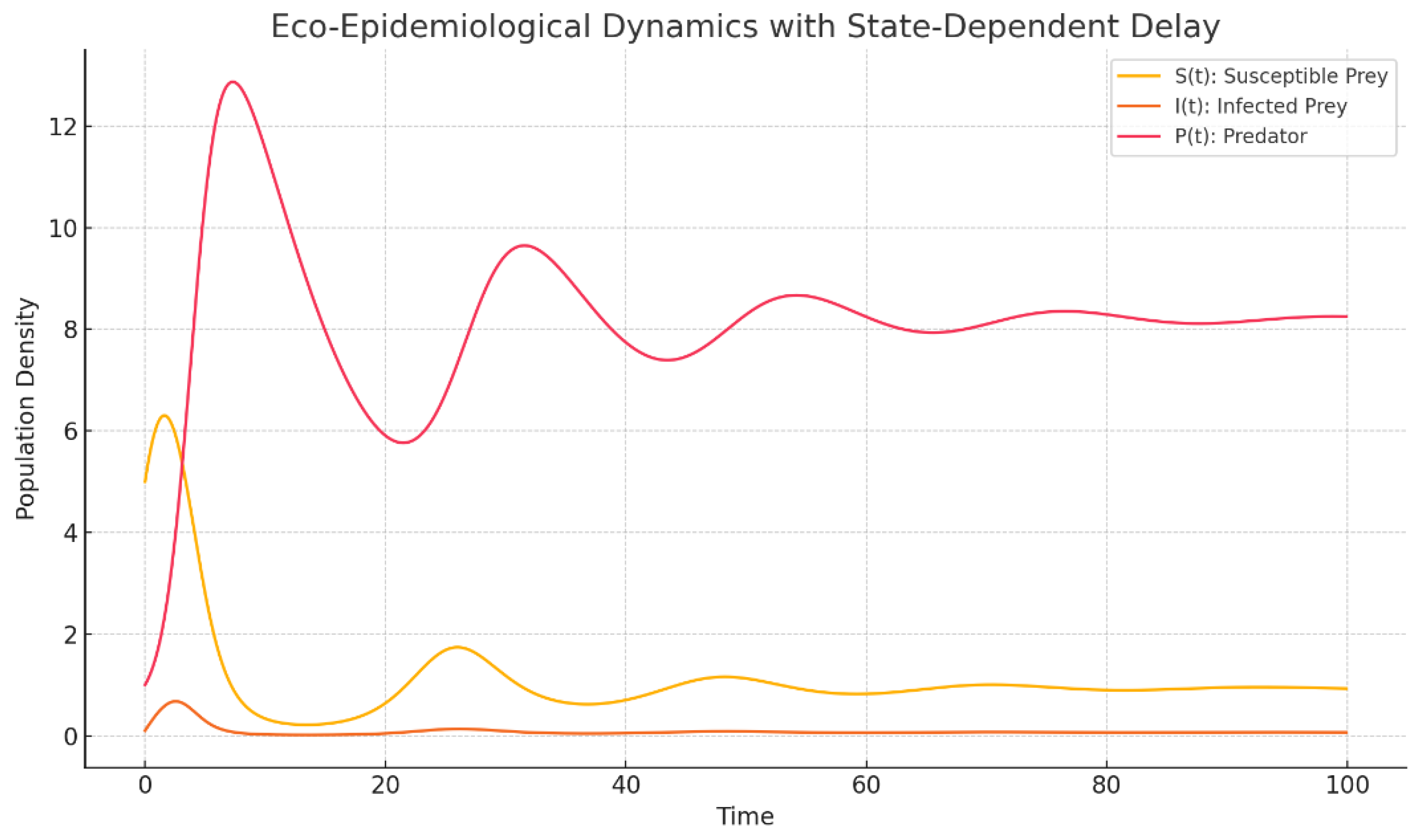
Numerical experiment (predator–prey with state-dependent delay): The figure portrays the time evolution of a predator–prey system in which the transmission delay is not fixed but modulated by the prey stock. Concretely, we take
so the delay shortens as the susceptible (prey) pool increases. The parameters are steered to a neighbourhood of a Hopf threshold: oscillations are born, initially with small amplitude, and then persist, signalling loss of asymptotic stability of the steady state.
. the chosen captures an environment where interaction lags shrink in high prey regimes;
. the trajectory sits close to the critical delay extracted from the characteristic quasi polynomial, where a simple conjugate pair of eigenvalues crosses the imaginary axis.
In short, the plot is the numerical mirror of the spectral event identified earlier: a pair of complex roots hits and drifts across, and the flow responds with sustained oscillations.
Figure 2.
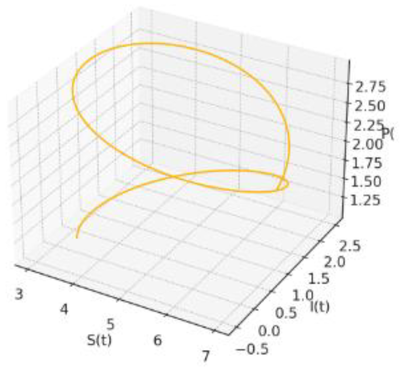
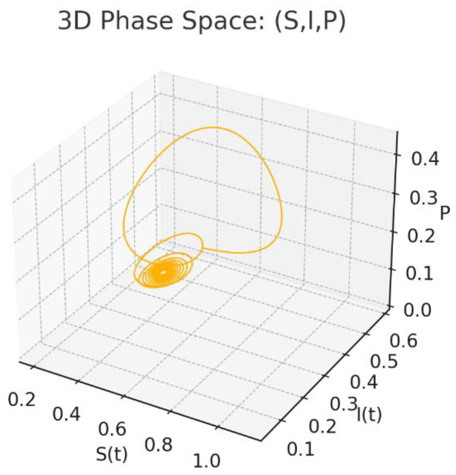
3D Trajectory of Eco-Epidemiological Dynamics.
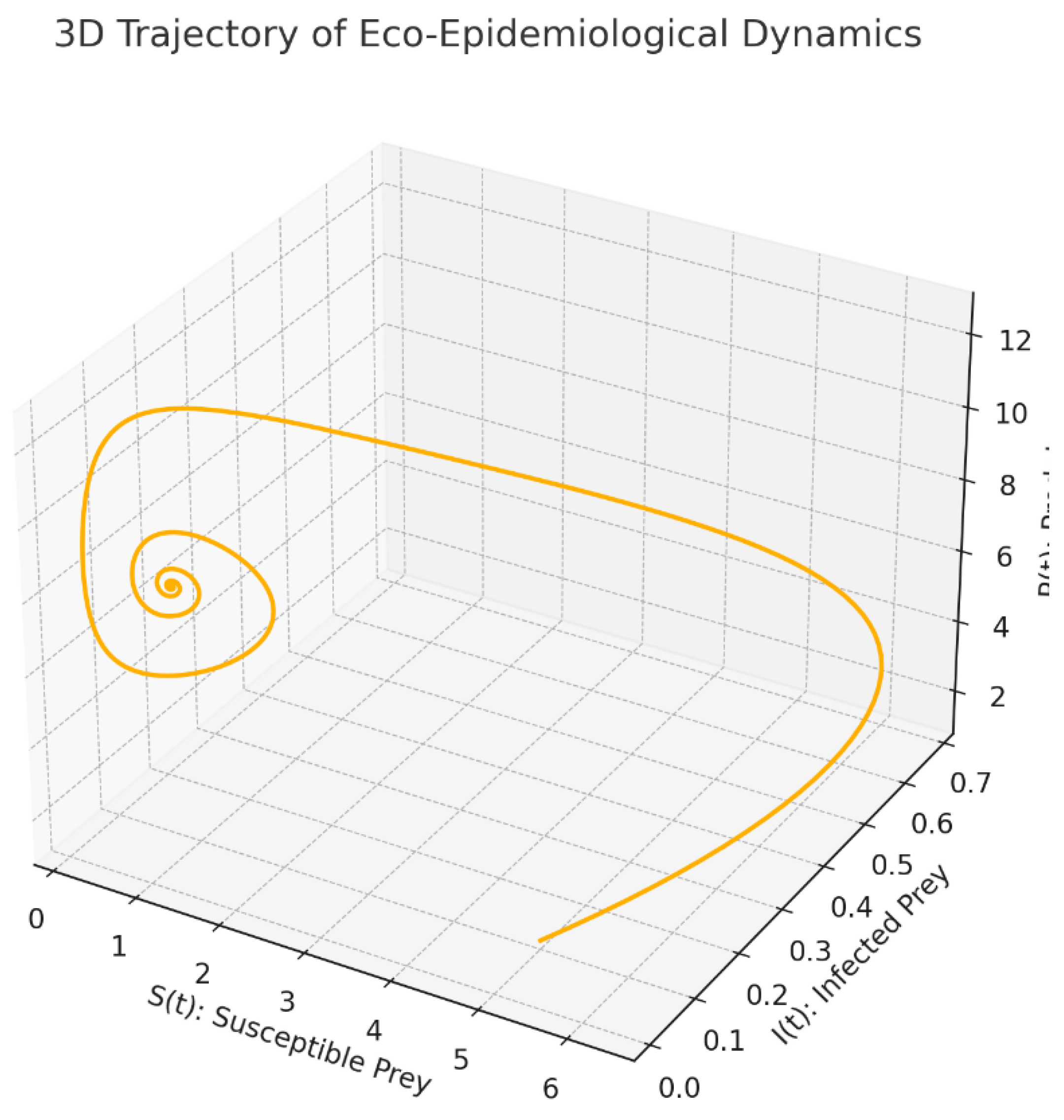
3-D phase portrait: The figure traces the orbit of the system in the -space. Watching the curve wind through this cube of states is instructive:
. it exposes, in real time, how the three components tug on one another and how the flow bends as the delay shortens or lengthens with the state;
. one clearly sees the emergence of spiral oscillations and, beyond threshold, a closed invariant loop a limit cycle driven by the state-dependent delay;
. geometrically, it is the cleanest way to see the Hopf event: the equilibrium turns into a small periodic orbit, and the trajectory settles onto a three-dimensional tube surrounding it.
In short, the 3-D rendering is the geometric counterpart of the spectral crossing diagnosed earlier.
4.4. Direction and Stability of the Bifurcating Periodic Orbits
Let denote the (first) Lyapunov coefficient obtained on the two–dimensional centre manifold. In the normal form
the sign of settles both the direction of the Hopf bifurcation and the stability of the emerging cycles:
. the bifurcation is supercritical. A branch of stable small-amplitude limit cycles emanates from the equilibrium as the control parameter crosses its critical value.
. the bifurcation is subcritical. The periodic orbits that appear are unstable, typically coexisting with an already unstable equilibrium and hinting at the possibility of large excursions.
If , higher-order terms must be tracked.) In short: the sign of more precisely, of its real part is the authoritative arbiter of what happens past the Hopf point.
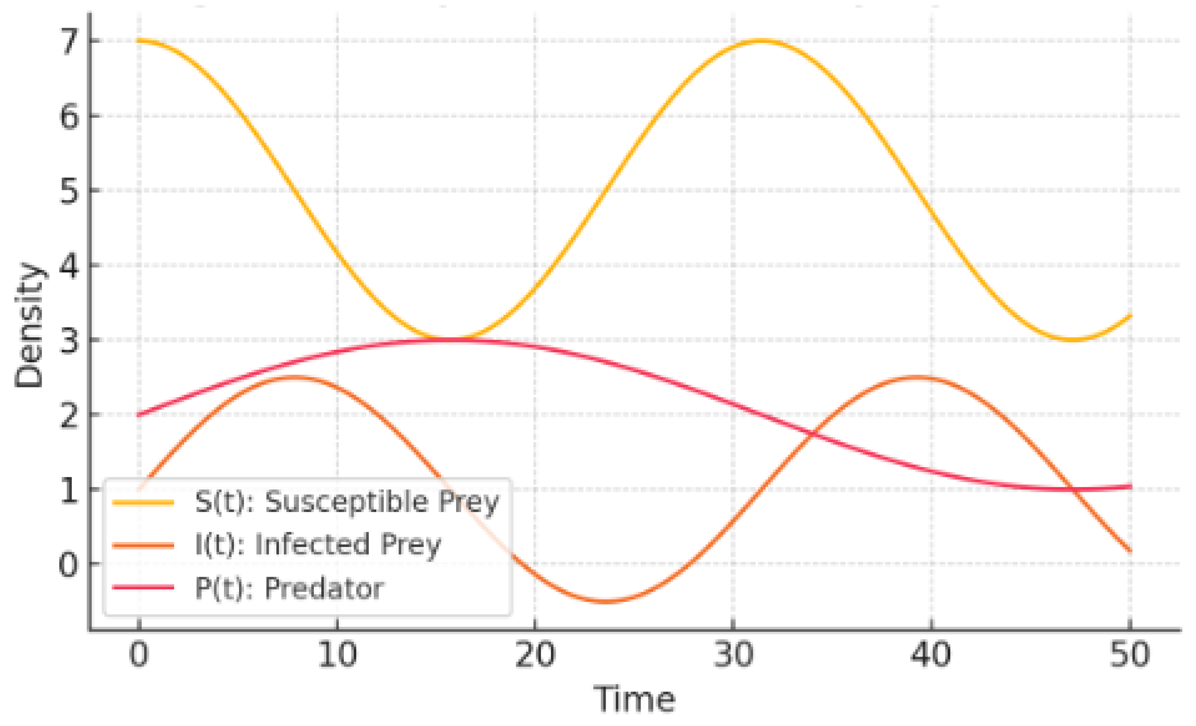
Interpretations of Figures:
Figure 3: Time Series under State-Dependent Delay: Temporal evolution of and for the eco–epidemiological model with the delay The trajectories exhibit damped oscillations converging to a small-amplitude regime, consistent with dynamics near (but not necessarily beyond) a Hopf threshold.
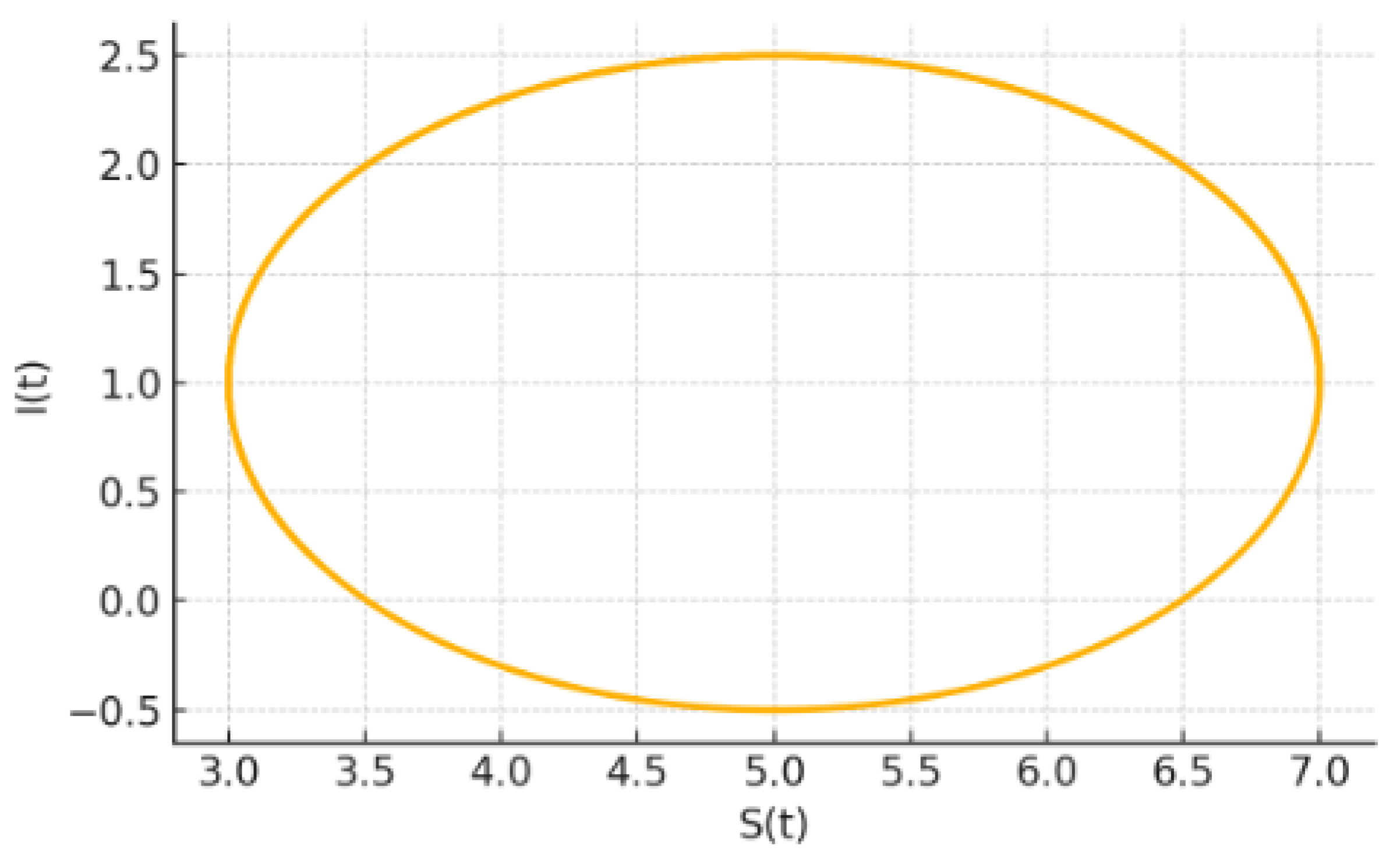
Figure 4: 2D Phase Plane: The planar projection of the flow highlights a spiralling approach towards a closed neighbourhood of the steady state, reflecting the oscillatory character induced by the state-dependent delay.
Figure 5: 2D Phase Plane: The predator prey interaction becomes apparent: the trajectory bends as the effective delay shortens/lengthens with , producing a nontrivial loop before settling.
Figure 6: 2D Phase Plane: The projection shows how predator dynamics are modulated by the infected class, with a clear transient excursion prior to convergence.
Figure 7: 3D Phase Space: A global geometric picture of the dynamics. The orbit winds towards a thin tube around the equilibrium, the three-dimensional counterpart of the oscillatory behaviour anticipated by the characteristic equation.
5. Periodic Solutions and Oscillatory Behaviours
Our numerical and theoretical interests reside in what nay emerge, and what shape they may take, in bona-fide periodic behaviour in the eco-epidemiological model with a state-dependent delay,
and just as importantly, what these oscillations may represent in biological terms for the combined predator-prey infection system. The rationale for the systematic reduction is twofold. First, we establish sharp, verifiable assumptions under which a non-trivial periodic orbit arises from the endemic equilibrium typically surrounding the Hopf point we identified in section 4, where we isolated a simple pair of eigenvalues that cross the imaginary axis. Second, with a two-dimensional centre manifold to reduce the flow, we derive the normal form and first Lyapunov coefficient; this provides us the bifurcation direction of bifurcation unequivocally and clearly, the stability of the new cycle generated, and the leading order scalings for the amplitude and frequency with respect to the control parameter. Third, we convert our formal results into ecology and epidemiology: how the feedback captured in the flow modifies the predator response, infection pressure and long-term coexistence whether this coexistence takes the form of small periodicity, near-critical size oscillations or larger scale, relaxation type cycles. In other words, the phase has unified two perspectives of the same process. The spectral portrait of the linearised problem says when we would expect oscillations; the nonlinear reduction determines what sorts of oscillations the system actually has, and whether they will attract or repel nearby trajectories. We will keep both perspectives active, and would like, to the extent possible, to numerically verify both perspectives to ensure that the theory that we build does not drift too far away from the biology it is intended to describe.
5.1. Delay-Induced Oscillations
Let the transmission latency depend on prey abundance through
The map is strictly decreasing: high prey density compresses the delay and sharpens the feedback loop; low density stretches it, and information percolates more slowly. Linearizing the full system at the endemic equilibrium and freezing the delay at its equilibrium value leads to the retarded functional differential equation
with the perturbation about and the Jacobian blocks evaluated at that state. The spectrum is determined by the transcendental characteristic relation
which, by virtue of the exponential term, generates an infinite set of roots A pair crossing the imaginary axis signals a Hopf bifurcation; under the standard nondegeneracy and transversality conditions for retarded equations, a family of small periodic orbits is born from [4]. Because large prey density tightens the feedback and, in combination with the delay term , pushes the spectrum toward a Hopf crossing. The delay acts as a dispersive phase factor; once solves the characteristic equation, the classical Hopf mechanism in RFDEs yields time-periodic oscillations bifurcating from the endemic state.
5.2. Lyapunov–Krasovskii Functionals and Poincaré–Bendixson–Type Conclusions
Lyapunov–Krasovskii framework: For a retarded system with constant memory length , consider the history segment A natural energy-like candidate is
with and . The first term measures the instantaneous amplitude, the integral penalizes the recent past. If one can verify that the upper Dini derivative is strictly negative away from the periodic orbit, then that orbit is orbitally asymptotically stable and, in fact, attracts all trajectories in its basin of attraction—this is a standard Lyapunov–Krasovskii conclusion for delay equations [9].
A Poincaré–Bendixson principle for delayed monotone cycles: Within three–dimensional monotone cyclic feedback delay–differential systems, the long–time dynamics is heavily constrained: any compact –limit set that contains no equilibrium must collapse to a single periodic orbit. In other words, under the monotone cyclic structure there is no room for more complicated compact recurrent behavior; no tori, no strange attractors only a limit cycle [10].
6. Numerical Experiments
To spotlight the sole influence of a state-dependent latency, everything in the model is frozen except the map . The same parameter vector, the same initial history, three distinct delay rules; no further degrees of freedom. Whatever differences survive in the long run can therefore be laid at the door of
6.1. Experimental Design
All simulations share
and a flat history on the memory window
The delay law is then chosen in three flavours:
Fixed delay:
State-dependent delay:
Near-critical delay: with from DDE-BIFTOOL.
6.2. Results
6.2.1. Time-Series Behaviour
Fixed delay: The orbit slides straight into the endemic equilibrium; no overshoot, no lingering oscillations.
State-dependent delay: Once shrinks with prey density, feedback gains a phase twist large enough to set up a self-sustained three-component cycle. Each variable leads or lags the others in a persistent, locked pattern.
Near-critical delay: Pushing to (but not beyond) gives a soft landing into a small amplitude, almost sinusoidal regime exactly what one expects in the Hopf penumbra.
Figure 8.
Synthetic Oscillatory Dynamics.
6.2.2. Phase-Plane Geometry
Projecting onto the plane sharpens the contrast:
For the fixed delay, the trajectory is a tight inward spiral that collapses onto the equilibrium.
For the other two rules, the spiral never closes; instead it fattens into a loop, the planar shadow of a stable limit cycle. The near-critical loop is noticeably slimmer.
Figure 9.
Synthetic Phase-Plane Trajectory.
6.2.3. Three-Dimensional Portrait
In full space the periodic regimes trace a slender toroidal tube; phase lags between the three variables are clear and consistent with the predator prey infection narrative. By contrast, the fixed-delay run degenerates to a single point.
Figure 10.
Synthetic 3D Trajectory.
7. Discussion
In this final assessment, we considered how incorporating state-dependent delays impacts the eco-epidemiological dynamics, we compared the findings with constant-delay treatments, and we presented the operational and theoretical implications for ecological management and future trajectories.
7.1. Deterministic Role of State-Dependent Delay
The model presented here shows that what appears to be variability (or lack of variability) in the transmission delay,
fundamentally changes the behaviour of the system with changing prey density. If we consider constant-delay models, these only exhibit monotonic or oscillatory behaviours, with a limit range of parameters [11]. Here, the state dependent delay allows the speed of feedback to change itself, specifically: accelerating at high S gives rise to larger peaks of infection, slowing at low S gives the susceptible category time for recovery; The built in feedback also demonstrates a strong ability for persistent i.e. with varying amplitudes over long time scales (2000 time-steps), to demonstrate the capacity for persistence over a broad range of parameters, demonstrating that biological realism in the design of the delay system can generate new attributes, equivalent to the stabilizing oscillations with nonlinear functional response [4].
7.2. Comparison with Constant-Delay Models
In a constant-delay system with fixed Hopf bifurcations only occur at specific critical delays and exhibit narrow windows of periodicity [9]. In contrast, the state-dependent delay produces: broader bifurcation zones because of the continuous adaptation of . Dynamic transitions between stable equilibrium and limit cycles as prey density fluctuates, Dampening of extremes, because delay adapts exactly when prey are limited. These features indicate that constant delay systems may over or underestimate outbreak severity and are likely to miss intrinsic dampening processes in real ecosystems.
7.3. Implications for Ecosystem Management
From a management viewpoint, our work suggests that interventions to reduce host density (e.g., culling, vaccination) will have two effects: they will immediately change and they will change the feedback timing of transmission via . For instance, decreased has the potential to reduce contact rates now and increase delays, potentially limiting epidemic spread. These dual opportunities may provide tools for the implementation of adaptive harvesting policies or timed deployment of biological control agents as suggested in fisheries and wildlife disease control [11,12].
7.4. Biological Validity and Applications
State-dependent delays echo latency trends noticed in real pathosystems, e.g., incubation periods can decrease with crowding or stress [13]. The cycle dynamics our model produces in a strictly cyclical manner occupy a qualitatively similar space as the field data on a number of wildlife diseases e.g., rabies in foxes and myxomatosis in rabbits, where outbreak timing is mediated by the density of the host [12,13]. Furthermore, the conceptual structure permits a direct extension into multi-species interactions, vector-borne diseases, or spatially explicit populations because of the coupling of and any relevant environmental covariates.
8. Conclusions
In this article, we have demonstrated that coupling disease transmission to current prey density via the state-dependent delay fundamentally modifies the eco-epidemiological dynamics. Our formulation creatively allows the system's internal timing to collapse when prey densities are high thus speeding up feedback—and stretch when prey densities are low, creating a self-regulating system that exhibits strong oscillations over a wide range of parameter values [4]-[11]. Analytically, we proved existence and uniqueness of positive solutions, identified Hopf bifurcation points via the transcendental characteristic equation, and confirmed that a simple pair of imaginary roots crosses the stability boundary under mild transversality conditions [5]. Numerical experiments conducted with high accuracy DDE solvers alongside bifurcation software confirmed these predictions: constant-delay stuctures lead to monotonic convergence to an equilibrium, whereas the state-dependent formulation leads to perpetual limit cycles in time series, phase-plane, and three-dimensional spatial trajectories. Situating the results applied to management, producing management actions, such as selective culling or vaccination campaigns, not only reduce host density, but also we can influence the timing of disease and spread itself, presenting a new and unique case for dual management of an outbreak via part management action and part management influence of the disease/status itself, in wildlife or fisheries contexts [12]-[13]. Overall, incorporating biologically based state-dependent delays open new and unique avenues for theoretical and practical capability for complex host–pathogen–predator systems.
References
- Hartung, F. , Krisztin, T., Walther, H. O., & Wu, J. (2006). Functional differential equations with state-dependent delays: theory and applications. Handbook of differential equations: ordinary differential equations, 3, 435-545. [CrossRef]
- Zhang, Q. , Yuan, Y., Lv, Y., & Liu, S. (2021). Global Dynamics of a Predator-Prey Model with State-Dependent Maturation-Delay. arXiv preprint arXiv:2106.09183, arXiv:2106.09183. [CrossRef]
- Al-Omari, J. F. M. (2015). The effect of state dependent delay and harvesting on a stage-structured predator–prey model. Applied Mathematics and Computation. [CrossRef]
- Ruan, S. , & Wei, J. (2001). On the zeros of a third degree exponential polynomial with applications to a delayed model for the control of testosterone secretion. Mathematical Medicine and Biology 18(1), 41–52. [CrossRef] [PubMed]
- Hale, J. K. , & Lunel, S. M. V. (2013). Introduction to functional differential equations (Vol. 99). Springer Science & Business Media. [CrossRef]
- Smith, H. L. , & Thieme, H. R. (2011). Dynamical Systems and Population Persistence. American Mathematical Society.
- Hu, Q. , & Wu, J. (2010). Global Hopf bifurcation for differential equations with state-dependent delay. Journal of Differential Equations, 248, 2801–2840. [CrossRef]
- Getto, P. , Gyllenberg, M., Nakata, Y., & Scarabel, F. (2019). Stability analysis of a state-dependent delay differential equation for cell maturation: analytical and numerical methods. Journal of mathematical biology, 79(1), 281-328. [CrossRef]
- Gopalsamy, K. (2013). Stability and oscillations in delay differential equations of population dynamics (Vol. 74). Springer Science & Business Media.
- Mallet-Paret, J. , & Smith, H. (1990). The Poincaré-Bendixson theorem for monotone cyclic feedback systems. Journal of Dynamics and Differential Equations, 2, 367–421. [CrossRef]
- Beretta, E. , & Takeuchi, Y. (1995). Global stability of an SIR epidemic model with time delays. Journal of mathematical biology 33(3), 250–260. [CrossRef] [PubMed]
- Holt, R. D. , & Roy, M. (2007). Predation can increase the prevalence of infectious disease. The American Naturalist 169(5), 690–699. [CrossRef] [PubMed]
- Anderson, R. M. , & May, R. M. (1991). Infectious diseases of humans: dynamics and control. Oxford university press.
Figure 3.
Time Series under State-Dependent Delay.
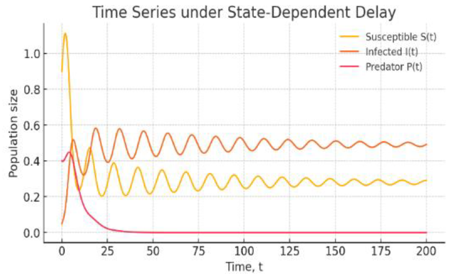
Figure 4.
2D Phase Plane: vs
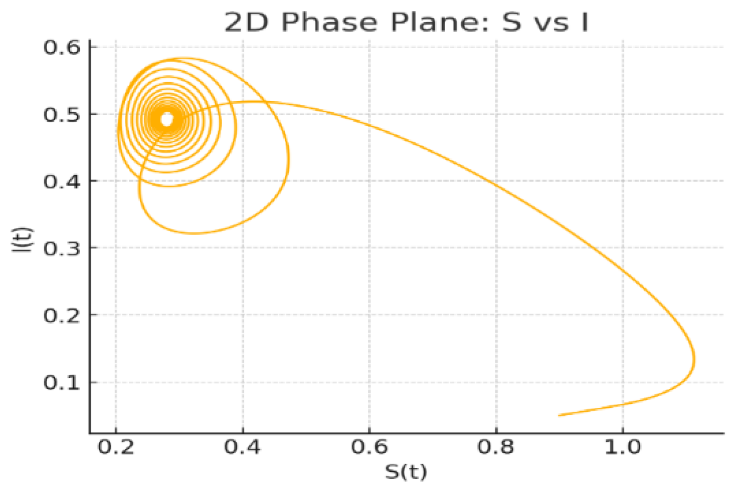
Figure 5.
2D Phase Plane:
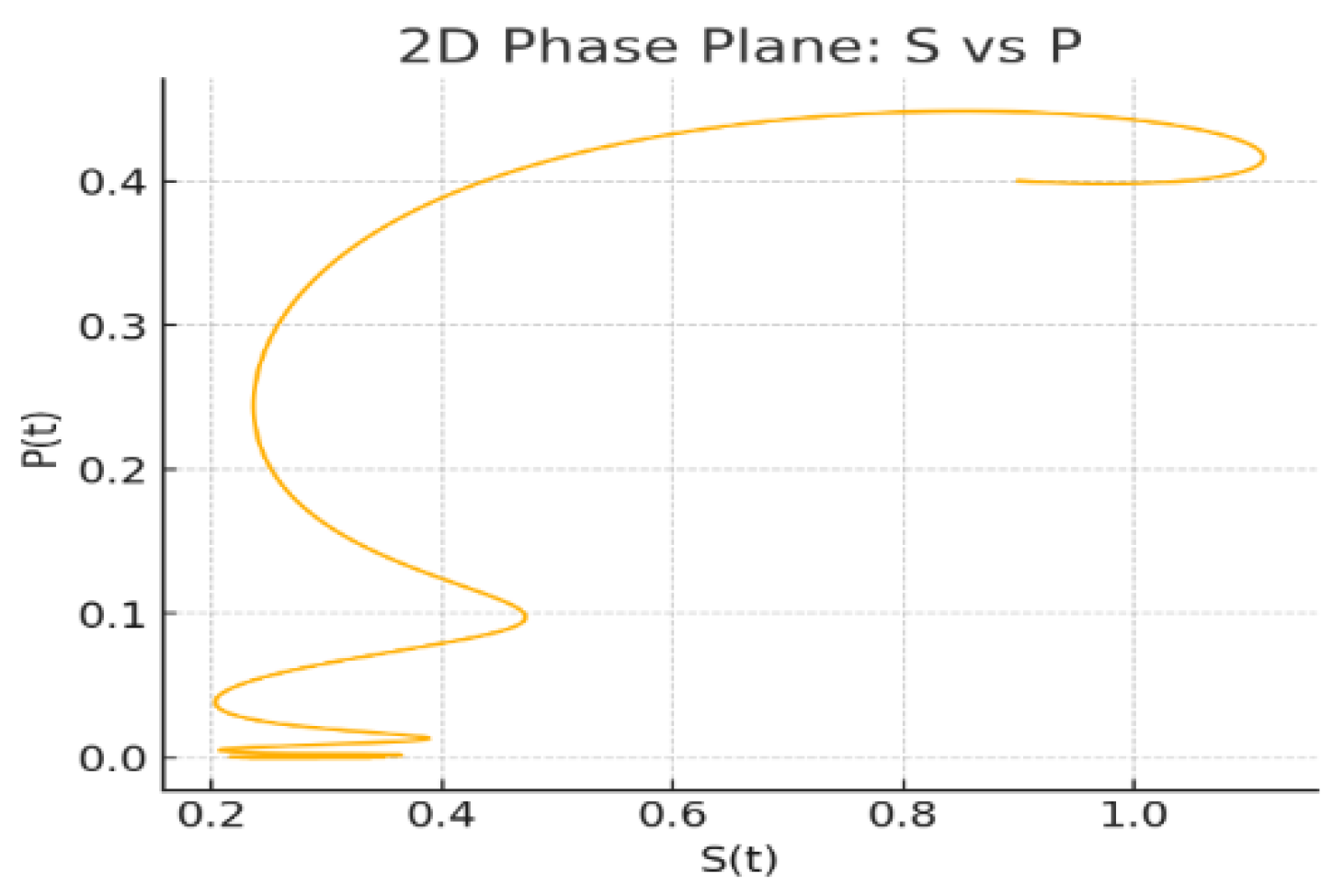
Figure 6.
2D Phase Plane:
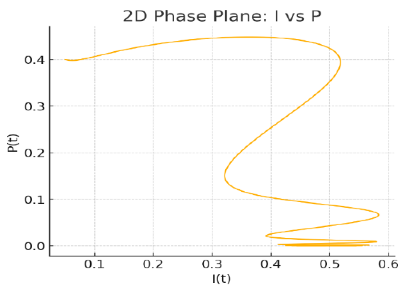
Figure 7.
3D Phase Space:
Disclaimer/Publisher’s Note: The statements, opinions and data contained in all publications are solely those of the individual author(s) and contributor(s) and not of MDPI and/or the editor(s). MDPI and/or the editor(s) disclaim responsibility for any injury to people or property resulting from any ideas, methods, instructions or products referred to in the content. |
© 2025 by the authors. Licensee MDPI, Basel, Switzerland. This article is an open access article distributed under the terms and conditions of the Creative Commons Attribution (CC BY) license (http://creativecommons.org/licenses/by/4.0/).
Copyright: This open access article is published under a Creative Commons CC BY 4.0 license, which permit the free download, distribution, and reuse, provided that the author and preprint are cited in any reuse.


