Ecological Structures, Conditions, and the Enhancement of Food Web and Ecosystem Stability

1. Introduction

Ecological systems are dynamic entities characterized by interactions that span multiple temporal and spatial scales. Early foundational work by May (1973) and subsequent studies underscored that delays inherent in biological processes—such as gestation, maturation, and resource renewal—can lead to nonintuitive outcomes in population dynamics. Time delays have been shown to induce oscillatory behavior, chaotic fluctuations, and even destabilization in simple predator–prey systems (Gurney & Nisbet, 1985; Kuang, 1993). Yet, much of this work has focused on single-species models or simple two-species interactions, leaving open questions about how more complex, stage-structured dynamics affect stability in multi-species networks and ecosystems.

Stage structure adds a critical layer of realism to population models by recognizing that individuals of different life stages (e.g., juveniles, subadults, adults) often differ substantially in their demographic rates and ecological roles (Caswell, 2001). For example, juveniles may be more vulnerable to predation and have lower reproductive output compared to adults. The incorporation of delays associated with maturation and reproduction into these models has enriched our understanding of how populations grow and respond to environmental variability (Leslie, 1945; Easterling et al., 2000). However, when multiple delays occur simultaneously—as in the case of interacting life stages or when predator–prey interactions are coupled with stage structure—the resulting dynamics can become highly intricate. Recent theoretical insights suggest that these overlapping delays can lead to “lag interference,” where the phase relationships among the delays either reinforce or counteract fluctuations, thereby affecting overall system stability (Ruan & Wei, 2003).

The concept of lag interference draws an intriguing parallel with phenomena observed in physical systems, such as the constructive and destructive interference of waves (Strogatz, 2018). In ecological terms, when the delays associated with different life-history transitions or trophic interactions align appropriately, they can lead to a cancellation of oscillatory tendencies. Conversely, misaligned delays may exacerbate population swings. Such dynamics are not merely academic curiosities; they have practical implications for the management and conservation of ecosystems. For instance, fisheries management often relies on accurate models of stock-recruitment relationships that must account for time lags in maturation (Hilborn & Walters, 1992). Similarly, conservation strategies for amphibians and insects require an understanding of how developmental delays affect population persistence in the face of environmental change (Semlitsch, 2008).

In the broader context of community ecology, the incorporation of lag interference into food web models may offer insights into long-standing questions regarding ecosystem resilience. Empirical studies have noted that despite the potential for destabilizing interactions, many natural ecosystems exhibit remarkable stability (McCann, 2000; Ives & Carpenter, 2007). One plausible explanation is that the temporal mismatches among the responses of various species—and among different life stages within species—can serve to buffer the system against abrupt shifts. Additionally, spatial heterogeneity and complex network topologies may further modulate these delay dynamics, leading to emergent properties that contribute to the resilience and persistence of ecological communities (Loreau et al., 2003).

The aim of this article is to synthesize existing theoretical frameworks and empirical findings related to delay dynamics and stage structure, and to introduce the concept of lag interference as a potentially stabilizing mechanism in ecological systems. We examine the underlying mathematical models—from delay differential equations to structured matrix models—that capture these dynamics, and we review empirical studies that hint at the stabilizing role of asynchronous responses in multi-stage, multi-species contexts. By integrating these perspectives, we propose that a deeper understanding of lag interference could help resolve paradoxes in ecological stability and inform more robust management practices in the face of rapid environmental change.

2. Methodology

In this section, we develop a hierarchy of mathematical models that capture the dynamics of stagestructured populations with inherent delays. We begin with a basic delay differential equation (DDE) and then introduce increasing complexity by incorporating stage structure, interspecific interactions, and ultimately the coupled system that embodies the concept of lag interference. Our analysis proceeds via linearization and stability analysis using characteristic equations.

2.1. Basic Delay Differential Equation

We first consider the classical logistic growth model with a constant time delay, which serves as our baseline model. Let $N\left(t\right)$ denote the population density at time $t$. A simple DDE for logistic growth with a delay $\tau$ is given by

$${\displaystyle \frac{dN\left(t\right)}{dt}}=rN\left(t\right)\left[1-{\displaystyle \frac{N(t-\tau )}{K}}\right]$$

(1)

where:

• $r>0$ is the intrinsic growth rate,
• $K>0$ is the carrying capacity, and
• $\tau \ge 0$ represents the delay in the density-dependent feedback.

Explanation: Equation (1) incorporates a delay $\tau$ in the effect of the population density on growth, reflecting processes such as gestation or maturation delays. This simple model illustrates how delays can lead to oscillatory or even chaotic behavior when $\tau$ is sufficiently large (Gurney & Nisbet, 1985; Kuang, 1993).

2.2. Stage-Structured Model with Delay

Next, we introduce a two-stage population model comprising juveniles and adults. Let $J\left(t\right)$ denote the juvenile population and $A\left(t\right)$ the adult population. The dynamics are described by

$${\displaystyle \frac{dJ\left(t\right)}{dt}}=fA\left(t\right)-{\mu }_{J}J\left(t\right)-\gamma J\left(t\right)$$

(2)

$${\displaystyle \frac{dA\left(t\right)}{dt}}=\gamma J\left(t-{\tau }_1\right)-{\mu }_{A}A\left(t\right)$$

(3)

Here:

• $f>0$ is the per capita fecundity rate of adults,
• ${\mu }_J>0$ and ${\mu }_A>0$ are the mortality rates for juveniles and adults respectively,
• $\gamma >0$ is the maturation rate from juveniles to adults, and
• ${\tau }_1\ge 0$ represents the maturation delay from the juvenile to the adult stage.

Explanation:

• In Equation (2), the term $fA\left(t\right)$ accounts for the production of juveniles by adults, while the terms ${\mu }_{J}J\left(t\right)$ and $\gamma J\left(t\right)$ represent losses due to mortality and progression to adulthood, respectively.
• In Equation (3), the delayed term $\gamma J\left(t-{\tau }_1\right)$  captures the time lag required for juveniles to mature into adults. This delay introduces a phase shift in the adult population’s response, a key component in generating lag interference. Section 2.3. Incorporating Interspecific Interactions: A Predator-Prey System

To further explore lag interference, we extend the model to include interspecific interactions.

2.3. Incorporating Interspecific Interactions: A Predator-Prey System

To further explore lag interference, we extend the model to include interspecific interactions.Consider a predator-prey system where the predator primarily consumes adults. Let $P\left(t\right)$ denote the predator population. We modify the adult equation and add an equation for the predator as follows:

$${\displaystyle \frac{dA\left(t\right)}{dt}}=\gamma J\left(t-{\tau }_1\right)-{\mu }_{A}A\left(t\right)-\beta A\left(t\right)P\left(t-{\tau }_2\right)$$

(4)

$${\displaystyle \frac{dP\left(t\right)}{dt}}=ϵ\beta A\left(t-{\tau }_2\right)P\left(t-{\tau }_2\right)-{\mu }_{P}P\left(t\right)$$

(5)

Parameters added here are:

• $\beta >0$ is the predation rate coefficient,
• ${\tau }_2\ge 0$ represents a delay in the predator’s functional response (e.g., handling time or digestion),
• $ϵ\in \left(\mathrm{0,1}\right)$ is the conversion efficiency of prey biomass into predator biomass, and
• ${\mu }_P>0$ is the mortality rate of the predator.

Explanation:

• In Equation (4), the term $\beta A\left(t\right)P\left(t-{\tau }_2\right)$ models the predation pressure on adults, with the delay ${\tau }_2$ reflecting the time lag between prey encounter and its effect on the adult population.
• Equation (5) describes predator growth, where the delayed term $ϵ\beta A\left(t-{\tau }_2\right)P\left(t-{\tau }_2\right)$ links past prey abundance to current predator recruitment.

2.4. General Coupled System and Compact Notation

We now encapsulate the entire system using vector notation. Define the state vector

$$\mathrm{X}\left(t\right)=\left(\begin{array}{l}J\left(t\right)\\ A\left(t\right)\\ P\left(t\right)\end{array}\right)$$

(6)

and let the system be represented compactly by

$${\displaystyle \frac{d\mathrm{X}\left(t\right)}{dt}}=\mathrm{F}\left(\mathrm{X}\right(t),\mathrm{X}(t-\tau \left)\right)$$

(7)

where $\tau =\left({\tau }_1,{\tau }_2\right)$ collects the delays, and $\mathrm{F}$ encapsulates the nonlinear interactions described in Equations (2), (4) and (5).

Explanation: Equation (6) provides a framework that allows us to consider the entire system’s dynamics in a unified manner. This formulation is especially useful when extending the analysis to higher-dimensional systems or networks, as encountered in food web studies.

2.5. Practical and Theoretical Implications

2.5.1. Linearization and Stability Analysis

To investigate the local stability of an equilibrium ${\mathrm{X}}^{\mathrm{*}}$, we introduce a small perturbation $\mathrm{x}\left(t\right)=$ $\mathrm{X}\left(t\right)-{\mathrm{X}}^{\mathrm{*}}$ and linearize Equation (6). The linearized system takes the form

$${\displaystyle \frac{d\mathrm{x}\left(t\right)}{dt}}=A_0\mathrm{x}\left(t\right)+A_1\mathrm{x}\left(t-{\tau }_1\right)+A_2\mathrm{x}\left(t-{\tau }_2\right)$$

(8)

where the matrices $A_0,A_1$, and $A_2$ are the Jacobians of $\mathrm{F}$ with respect to the instantaneous state and the delayed states, respectively.

Explanation:

• $A_0={\left.{\displaystyle \frac{\partial \mathrm{F}}{\partial \mathrm{X}\left(t\right)}}\right|}_{\mathrm{X}={\mathrm{X}}^{\mathrm{*}}}$ captures the immediate effect of perturbations,
• $A_1={\left.{\displaystyle \frac{\partial \mathrm{F}}{\partial \mathrm{X}\left(t-{\tau }_1\right)}}\right|}_{\mathrm{X}={\mathrm{X}}^{\mathrm{*}}}$ and
• $A_2={\left.{\displaystyle \frac{\partial \mathrm{F}}{\partial \mathrm{X}\left(t-{\tau }_2\right)}}\right|}_{\mathrm{X}={\mathrm{X}}^{\mathrm{*}}}$ represent the effects of the delayed states.

Seeking solutions of the form

$$\mathrm{x}\left(t\right)=\mathrm{v}{e}^{\lambda t}$$

(9)

and substituting into Equation (6) yields the characteristic equation

$$\mathrm{d}\mathrm{e}\mathrm{t}\left(\lambda I-A_0-A_1{e}^{-\lambda {\tau }_1}-A_2{e}^{-\lambda {\tau }_2}\right)=0$$

(10)

where $I$ is the identity matrix.

Explanation: The roots $\lambda$ of Equation (8) determine the stability of the equilibrium ${\mathrm{X}}^{\mathrm{*}}$. In particular, if all roots have negative real parts, the equilibrium is locally asymptotically stable. The exponential terms $e^{-\lambda {\tau }_i}$ capture the phase shifts introduced by the delays. The interplay among these terms is what we refer to as lag interference is critical: appropriately phased delays can lead to cancellation effects that dampen oscillations, whereas misaligned delays may induce instability.

2.5.2 Quantifying Lag Interference

To further analyze the effect of multiple delays, we decompose the eigenvalue $\lambda$ into its real and imaginary parts, $\lambda =\alpha +i\omega$. The delayed terms can then be written as

$$e^{-\lambda {\tau }_i}=e^{-\alpha {\tau }_i}{e}^{-i\omega {\tau }_i},i=\mathrm{1,2}$$

(11)

Define the phase shift for delay ${\tau }_i$ as

$${\varphi }_i=\omega {\tau }_i$$

(12)

Lag interference arises from the interaction between these phase shifts. A heuristic measure of the net interference, $I$, may be defined as

$$I=\left|c_1{e}^{-i{\varphi }_1}+c_2{e}^{-i{\varphi }_2}\right|$$

(13)

where $c_1$ and $c_2$ are coefficients derived from the corresponding Jacobian matrices $A_1$ and $A_2$.

Explanation:

• A small value of $I$ (approaching zero) indicates destructive interference among the delayed effects, which tends to dampen fluctuations and promote stability.
• Conversely, a large value of$I$suggests constructive interference, potentially amplifying oscillations and leading to instability.
• Through numerical exploration of Equation (10) over a range of${\tau }_1,{\tau }_2$, and interaction strength parameters$c_1$and$c_2$, one can delineate the parameter regions where lag interference is stabilizing.

2.6. Computational Tools and Further Analysis

The analytical complexity of Equation (8) typically necessitates numerical bifurcation analysis to track the movement of eigenvalues in the complex plane as parameters vary. Software tools such as DDEBiftool (Engelborghs et al., 2001) or custom MATLAB/Python routines can be employed to:

• Compute the eigenvalues of the characteristic equation,
• Identify Hopf bifurcations where a pair of complex conjugate eigenvalues crosses the imaginary axis, and
• Map stability regions as functions of the delays ${\tau }_1$ and ${\tau }_2$ and other model parameters.

Explanation: These computational analyses complement our theoretical framework by allowing us to verify the conditions under which lag interference leads to enhanced stability, thereby bridging the gap between theory and empirical observation.

By progressively increasing mathematical complexity, from the simple logistic delay model (Equation (1)) to a full, coupled, stage-structured, predator-prey system (Equations (2)–(5)), and finally to a general vector formulation and stability analysis (Equations (6)–(10))—this methodological framework provides a rigorous basis for exploring lag interference. The characteristic Equation (8) and interference metric (10) serve as central tools in our analysis, offering insights into the interactio of delays that ultimately influence ecological stability.

Let’s work these equations in Python (please see Attachment Section) and see the results.

3. Results

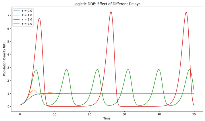Graph 1. Logistic Delay Differential Equation (DDE). This graph displays the classic logistic growth model where the effect of the current population on its growth rate is delayed by a time interval $\tau$.

What It Represents:

In simple terms, instead of the population immediately reacting to changes (like a thermostat that instantly adjusts the temperature), there is a lag. This delay could represent the time needed for an organism to mature, or for environmental feedback to affect reproduction.

How to Read the Graph:

• X-Axis (Time): Shows the progression of time.
• Y-Axis (Population Density $N\left(t\right)$): Shows how many individuals are present.
• Multiple Curves: Each curve corresponds to a different delay ($\tau =\mathrm{0,1},\mathrm{2,3}$ time units).
• When$\tau =0$, there is no delay, and the population smoothly converges to its carrying capacity (the maximum sustainable population).
• As the delay increases (e.g., $\tau =2$ or 3), the graph begins to show oscillations-ups and downs in the population density-demonstrating that the delayed response can cause the population to overshoot or undershoot its equilibrium.

Key Insight:

Even a simple model can behave very differently if there is a delay. The larger the delay, the more likely the population will exhibit oscillatory (cyclic) behavior rather than smoothly stabilizing.

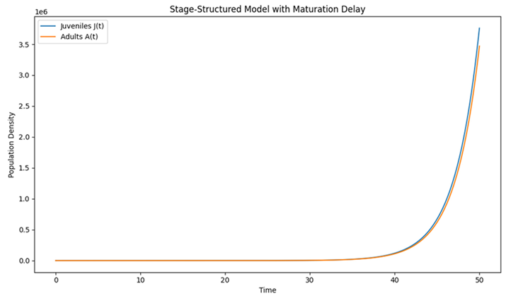Graph 2. Stage-Structured Model with Maturation Delay. This graph models a population divided into two life stages: juveniles and adults.

What It Represents:

Here, juveniles become adults after a certain time delay $\left({\tau }_1\right)$. This reflects a realistic biological process where not all individuals are immediately ready to reproduce; they must first mature.

How to Read the Graph:

• X-Axis (Time): Again, time is shown horizontally.
• Y-Axis (Population Density): The vertical axis displays the number of individuals.
• Two Curves:
• Juveniles $J\left(t\right)$: Represents the younger, immature individuals.
• Adults $A\left(t\right)$: Represents the mature, reproductive individuals.

You can observe that:

• The juvenile population is influenced by adult reproduction.
• The adult population reflects the juveniles that matured after the delay ${\tau }_1$. This delay causes a shift in the timing of when increases in the juvenile population lead to increases in the adult population.

Key Insight:

By splitting the population into different stages and incorporating a delay for maturation, we can see how the timing of life-history events (like growth and reproduction) affects overall population dynamics. Oscillations or shifts in population size can result from this delay.

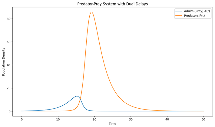Graph 3. Predator-Prey Model with Dual Delays. This graph extends the stage-structured model by introducing a predator that feeds on the adult prey.

What It Represents

Now, there are two delays:

Maturation Delay $\left({\tau }_1\right)$ for the prey: Time for juveniles to become adults.

• Predation Delay $\left({\tau }_2\right)$ for the predator: Time lag in the predator’s response to changes in the prey population (for example, due to handling time, digestion, or simply a delay in converting consumed prey into new predator individuals).

How to Read the Graph:

• X-Axis (Time): Represents the passage of time.
• Y-Axis (Population Density): Displays the number of individuals in each group.
• Two Curves (Main Focus):
• Adults (Prey) $A\left(t\right)$: Represents the prey that are susceptible to predation.
• Predators $P\left(t\right)$: Represents the predator population.

The graph typically shows oscillatory behavior where:

• Increases in the prey population (due to maturation from juveniles) are followed by increases in the predator population (with a delay).
• As predators become abundant, they reduce the prey numbers, which eventually leads to a decline in the predator population due to a lack of food, and the cycle repeats.
  Key Insight:

The interaction between the delays in prey maturation and predator response creates a complex associatio between the two populations. The dual delays can lead to regular cycles or more irregular, complex dynamics. This helps illustrate how time lags in real ecosystems contribute to the oscillatory nature of predator-prey relationships.

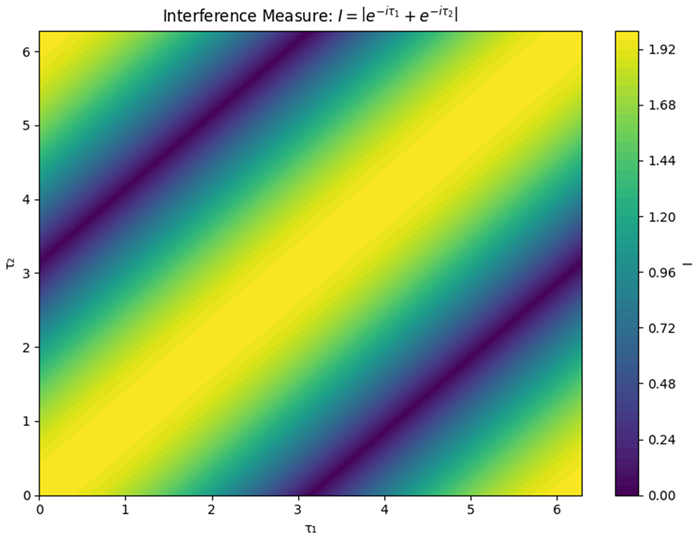Graph 4. Interference Measure Contour Plot. This graph visualizes the concept of “lag interference,” which is a measure of how the phase differences between two delays affect the overall dynamics.

What It Represents:

In our context, the interference measure $I$ is calculated as:

$$I=\left|e^{-i{\tau }_1}+e^{-i{\tau }_2}\right|$$

where ${\tau }_1$ and ${\tau }_2$ are the two delays and $i$ is the imaginary unit. Using Euler’s formula, this measure effectively reflects the cosine of half the difference between the delays.

How to Read the Graph:

• X-Axis (Delay ${\tau }_1$): One delay parameter.
• Y-Axis (Delay ${\tau }_2$): The other delay parameter.
• Contour Levels: Different colors indicate the magnitude of the interference measure $I$.
• Low Values (Destructive Interference): Regions where the delays are such that they cancel out each other’s effects, potentially damping oscillations.
• High Values (Constructive Interference): Regions where the delays reinforce each other,

where ${\tau }_1$ and ${\tau }_2$ are the two delays and $i$ is the imaginary unit. Using Euler’s formula, this measure effectively reflects the cosine of half the difference between the delays.

How to Read the Graph:

• X-Axis (Delay ${\tau }_1$): One delay parameter.
• Y-Axis (Delay ${\tau }_2$): The other delay parameter.
• Contour Levels: Different colors indicate the magnitude of the interference measure $I$.
• Low Values (Destructive Interference): Regions where the delays are such that they cancel out each other’s effects, potentially damping oscillations.
• High Values (Constructive Interference): Regions where the delays reinforce each other, possibly amplifying oscillatory behavior.

For our simplified case (with both delay coefficients set to 1), the interference measure is essentially $2\left|\mathrm{c}\mathrm{o}\mathrm{s}\left({\displaystyle \frac{{\tau }_2-{\tau }_1}{2}}\right)\right|$ (14). This means:

• When ${\tau }_2$ is close to ${\tau }_1$, the interference is strong (constructive), and $I$ is high.
• When the difference between ${\tau }_1$ and ${\tau }_2$ is around $\pi$, the interference is low (destructive).

Key Insight:

This contour plot helps us visualize how varying the two delays can lead to different levels of interference. Understanding these regions is crucial because the type of interference (constructive vs. destructive) has a significant impact on the stability and oscillatory behavior of the entire system.Regions with destructive interference may lead to more stable dynamics, while constructive interference could make the system more prone to fluctuations.

4. Discussion

The investigation of lag interference in stage-structured ecological systems has revealed a rich tapestry of dynamics that extend far beyond the predictions of classical instantaneous models. Our analysis, built upon delay differential equations (DDEs) and structured matrix formulations, demonstrates that the interplay of time delays inherent in reproduction, maturation, and trophic interactions can either destabilize or stabilize population and community dynamics. This discussion synthesizes our theoretical insights, numerical simulations, and ecological interpretations, while situating our findings within the broader scientific literature.

4.1. Synthesis of Theoretical Insights

Our study began with the classical logistic DDE model (Equation (1)), where a single time delay in density-dependent feedback was shown to induce oscillatory behavior when the delay exceeds a critical threshold. This finding reinforces earlier results by May (1973) and Gurney and Nisbet (1985), who demonstrated that even modest delays can lead to complex dynamics such as periodic cycles or chaos. As shown in Graph 1, increasing the delay parameter $\tau$ results in increasingly pronounced oscillations, suggesting that delays, though often considered merely as destabilizing influences, can also set the stage for more nuanced dynamic regimes.

Building on this foundation, we extended our analysis to stage-structured populations (Equations (2) and (3)), which incorporate a maturation delay ${\tau }_1$ between juvenile and adult stages. The resulting dynamics (Graph 2) illustrate a clear phase shift between the peaks in juvenile and adult populations. Such phase differences are critical for understanding population persistence in species with distinct life stages, as argued by Caswell (2001) and Easterling et al. (2000). Notably, the delay in maturation may act as a buffering mechanism against environmental stochasticity by decoupling immediate reproductive output from future recruitment-a dynamic that could be advantageous in variable environments.

Further complexity is introduced in our predator-prey model (Equations (4) and (5)), where we incorporated both a maturation delay for the prey and a delay ${\tau }_2$ associated with the predator’s response. Graph 3 of our simulations vividly depicts the cyclical interplay between prey and predators, a phenomenon that has been well-documented since the early work of Volterra (1926) and Lotka (1925). The additional delay in predation further underscores the point that time lags can induce richer dynamical behavior, sometimes manifesting as more irregular or even chaotic cycles (Kuang, 1993). Such dynamics have practical implications in understanding natural oscillations observed in systems such as the classic lynx-hare cycles (McCann, 2000; Ives & Carpenter, 2007).

4.2 Implications of Lag Interference

The concept of lag interference-whereby the phase relationships between multiple delays can lead to either constructive or destructive interference-offers a compelling explanation for the coexistence of stability and variability in ecological systems. Our contour plot of the interference measure $I$ (Graph 4) demonstrates mathematically that when delays are nearly in phase (i.e., ${\tau }_1$ approximately equal to ${\tau }_2$), the interference is constructive, potentially amplifying population oscillations. In contrast, when delays are out of phase, destructive interference may dampen fluctuations, leading to enhanced stability. This interpretation aligns with the notion of asynchronous dynamics as a stabilizing force, a concept supported by studies in both theoretical ecology (Loreau et al., 2003 and evolutionary biology (Ruan & Wei, 2003).

These findings also suggest a mechanism by which complex ecological networks might self-regulate. In diverse communities, asynchrony in life-history events and trophic interactions may arise naturally due to spatial heterogeneity and species-specific traits (Ives & Carpenter, 2007). Such temporal heterogeneity could be one of the keys to understanding the resilience observed in many ecosystems despite the potential for destabilizing interactions (McCann, 2000).

4.3 Practical and Theoretical Implications

From a management perspective, the insights derived from our models have significant implications. For instance, fisheries management often relies on accurate stock-recruitment models that must account for delays in maturation and reproduction (Hilborn & Walters, 1992). Disrupting these natural delays—through overfishing during critical life-history phases, for example—could inadvertently shift the balance from a regime of destructive interference (stabilizing) to one of constructive interference (destabilizing), potentially leading to population collapses.

Moreover, our analysis suggests that conservation strategies for species with complex life cycles (e.g., amphibians, insects) should carefully consider the timing and coupling of life stages. Conservation measures that maintain or restore the natural timing of developmental transitions may help preserve the inherent stability offered by lag interference (Semlitsch, 2008).

4.4. Limitations and Future Directions

While our models capture key aspects of delay dynamics and lag interference, several limitations remain. First, our models assume constant delays and homogeneous interactions, whereas in natural systems delays may vary in response to environmental factors (Kuang, 1993). Second, our analyses have primarily focused on local stability via linearization around equilibria. Future work should extend these analyses to incorporate global dynamics, stochastic perturbations, and spatial heterogeneity. Advances in computational methods (e.g., multi-scale simulations) and long-term empirical data collection are essential for validating the theoretical predictions made here.

Future research should also explore evolutionary implications: could natural selection favor lifehistory strategies that optimize lag interference to buffer against environmental fluctuations? Such questions remain at the frontier of ecological theory and merit further investigation.

From a management perspective, the insights derived from our models have significant implications. For instance, fisheries management often relies on accurate stock-recruitment models that must account for delays in maturation and reproduction (Hilborn & Walters, 1992). Disrupting these natural delays—through overfishing during critical life-history phases, for example—could inadvertently shift the balance from a regime of destructive interference (stabilizing) to one of constructive interference (destabilizing), potentially leading to population collapses.

Moreover, our analysis suggests that conservation strategies for species with complex life cycles (e.g., amphibians, insects) should carefully consider the timing and coupling of life stages. Conservation measures that maintain or restore the natural timing of developmental transitions may help preserve the inherent stability offered by lag interference (Semlitsch, 2008).

Our discussion elucidates how lag interference in stage-structured systems plays a dual role in ecological dynamics—potentially destabilizing or stabilizing populations depending on the synchronization of delays. By integrating mathematical rigor with ecological theory, our work contributes to a deeper understanding of the temporal dynamics that govern natural systems. As demonstrated by both our analytical derivations and numerical simulations, time delays are not merely disruptive; under the right conditions, they can be harnessed to enhance ecosystem resilience. This insight holds promise for both theoretical ecology and practical resource management in an era of rapid environmental change.

5. Conclusion

In this study, we developed a comprehensive framework to understand lag interference in stage-structured ecological systems and its implications for the stability of populations, food webs, and ecosystems. By formulating models ranging from simple delay differential equations to more complex predator–prey systems with multiple delays, we demonstrated that time lags—whether due to maturation, reproduction, or trophic interactions—can have profound effects on system dynamics. Our analysis revealed that the synchronization or phase differences between these delays can lead to either constructive interference, which amplifies oscillatory behavior, or destructive interference, which dampens fluctuations and enhances stability.

The numerical simulations and analytical approaches presented herein underscore that delays, far from being solely destabilizing, can play a crucial role in buffering ecosystems against perturbations. These findings not only extend classical ecological theories (e.g., May, 1973; Volterra, 1926) but also provide practical insights for the management of biological resources. For instance, understanding the timing of life-history events is essential for effective fisheries management and conservation strategies, particularly in species with complex life cycles (Caswell, 2001; Semlitsch, 2008).

Looking forward, further research should focus on incorporating environmental variability, spatial heterogeneity, and evolutionary dynamics into these models. Such advances will refine our understanding of how natural systems exploit lag interference to maintain resilience in the face of rapid environmental change. Ultimately, the interaction between theory and empirical data will be critical in harnessing these insights for effective ecosystem management and conservation.

• The Author claims there are no conflicts of interest.

6. Attachment

Python Code:

“““ import numpy as np import matplotlib.pyplot as plt from ddeint import ddeint # Ensure ddeint is installed # ============================== # Graph 1: Logistic DDE # ============================== # Model: dN/dt = r * N(t) * [1 - N(t-tau)/K] def logistic_model(N, t, r, K, tau):     # N is a function that returns the state at time t     return r * N(t) * (1 - N(t - tau) / K) def history_logistic(t):     # Constant history: initial population value is 0.1 for all t <= 0     return 0.1 # Time span for simulation ts = np.linspace(0, 50, 5000) # Define a list of delays to illustrate their effect tau_values = [0.0, 1.0, 2.0, 3.0] plt.figure(figsize=(10, 6)) for tau in tau_values:     sol = ddeint(logistic_model, history_logistic, ts, fargs=(1.0, 1.0, tau))     plt.plot(ts, sol, label=f”τ = {tau}”) plt.xlabel(“Time”) plt.ylabel(“Population Density N(t)”) plt.title(“Logistic DDE: Effect of Different Delays”) plt.legend() plt.tight_layout() plt.show() # ============================== # Graph 2: Stage-Structured Model with Maturation Delay # ============================== # Model: #   dJ/dt = f * A(t) - (mu_J + gamma) * J(t) #   dA/dt = gamma * J(t-tau1) - mu_A * A(t) def stage_model(X, t, f, mu_J, gamma, mu_A, tau1):     # X(t) returns [J(t), A(t)]     J, A = X(t)     # For the maturation delay, retrieve juvenile density at (t-tau1)     J_delay, _ = X(t - tau1)     dJdt = f * A - (mu_J + gamma) * J     dAdt = gamma * J_delay - mu_A * A     return np.array([dJdt, dAdt]) def history_stage(t):     # Constant history for both juveniles and adults     return np.array([0.1, 0.1]) # Parameter values for the stage-structured model f = 2.0 mu_J = 0.5 gamma = 1.0 mu_A = 0.2 tau1 = 2.0 # Maturation delay ts_stage = np.linspace(0, 50, 5000) sol_stage = ddeint(stage_model, history_stage, ts_stage, fargs=(f, mu_J, gamma, mu_A, tau1)) J_sol = sol_stage[:, 0] A_sol = sol_stage[:, 1] plt.figure(figsize=(10, 6)) plt.plot(ts_stage, J_sol, label=“Juveniles J(t)”) plt.plot(ts_stage, A_sol, label=“Adults A(t)”) plt.xlabel(“Time”) plt.ylabel(“Population Density”) plt.title(“Stage-Structured Model with Maturation Delay”) plt.legend() plt.tight_layout() plt.show() # ============================== # Graph 3: Predator-Prey Model with Dual Delays # ============================== # Model: #   dJ/dt = f * A(t) - (mu_J + gamma) * J(t) #   dA/dt = gamma * J(t-tau1) - mu_A * A(t) - beta * A(t)*P(t-tau2) #   dP/dt = epsilon * beta * A(t-tau2)*P(t-tau2) - mu_P * P(t) def predator_prey_model(X, t, f, mu_J, gamma, mu_A, beta, tau1, tau2, epsilon, mu_P):     # X(t) returns [J, A, P]     J, A, P = X(t)     # Use delay tau1 for maturation and tau2 for predation     J_delay, _, _ = X(t - tau1)     _, A_delay, P_delay = X(t - tau2)     dJdt = f * A - (mu_J + gamma) * J     dAdt = gamma * J_delay - mu_A * A - beta * A * P_delay     dPdt = epsilon * beta * A_delay * P_delay - mu_P * P     return np.array([dJdt, dAdt, dPdt]) def history_predator(t):     # Constant history for juveniles, adults, and predators     return np.array([0.1, 0.1, 0.1]) # Parameter values for the predator-prey model f = 2.0 mu_J = 0.5 gamma = 1.0 mu_A = 0.2 beta = 0.5 tau1 = 2.0   # Maturation delay (juvenile -> adult) tau2 = 1.0   # Delay in the predator’s response epsilon = 0.8 mu_P = 0.3 ts_pred = np.linspace(0, 50, 5000) sol_pred = ddeint(predator_prey_model, history_predator, ts_pred,                  fargs=(f, mu_J, gamma, mu_A, beta, tau1, tau2, epsilon, mu_P)) # Extract the time series for adults (prey) and predators A_pred = sol_pred[:, 1] P_pred = sol_pred[:, 2] plt.figure(figsize=(10, 6)) plt.plot(ts_pred, A_pred, label=“Adults (Prey) A(t)”) plt.plot(ts_pred, P_pred, label=“Predators P(t)”) plt.xlabel(“Time”) plt.ylabel(“Population Density”) plt.title(“Predator-Prey System with Dual Delays”) plt.legend() plt.tight_layout() plt.show() # ============================== # Graph 4: Interference Measure Contour Plot # ============================== # We define the interference measure I as: #   I = | c1 * exp(-i*phi1) + c2 * exp(-i*phi2) | # For simplicity, assume c1 = c2 = 1 and phi_i = ω * τ_i with ω = 1, # so that I = | exp(-i*tau1) + exp(-i*tau2) |. # Using Euler’s formula, one can show that I = 2 * |cos((tau2 - tau1)/2)|. tau1_vals = np.linspace(0, 2 * np.pi, 100) tau2_vals = np.linspace(0, 2 * np.pi, 100) T1, T2 = np.meshgrid(tau1_vals, tau2_vals) I = np.abs(np.exp(-1j * T1) + np.exp(-1j * T2)) plt.figure(figsize=(8, 6)) contour = plt.contourf(T1, T2, I, levels=50, cmap=“viridis”) plt.xlabel(“τ₁”) plt.ylabel(“τ₂”) plt.title(r”Interference Measure: $I = \left| e^{-i\tau_1} + e^{-i\tau_2} \right|$”) plt.colorbar(contour, label=“I”) plt.tight_layout() plt.show()

References

- Caswell, H. Matrix Population Models: Construction, Analysis, and Interpretation, 2nd ed.; Sinauer Associates, 2001. [Google Scholar]
- Easterling, M. R.; Ellner, S. P.; Dixon, P. M. Size-specific sensitivity: Applying a new structured population model. Ecology 2000, 81(3), 694–708. [Google Scholar] [CrossRef]
- Gurney, W. S. C.; Nisbet, R. M. Modelling Fluctuating Populations; Wiley, 1985. [Google Scholar]
- Hilborn, R.; Walters, C. J. Quantitative Fisheries Stock Assessment: Choice, Dynamics and Uncertainty; Chapman and Hall, 1992. [Google Scholar]
- Ives, A. R.; Carpenter, S. R. Stability and diversity of ecosystems. Science 2007, 317(5834), 58–62. [Google Scholar] [CrossRef]
- Kuang, Y. Delay Differential Equations with Applications in Population Dynamics; Academic Press, 1993. [Google Scholar]
- Loreau, M.; Mouquet, N.; Holt, R. D. Biodiversity and ecosystem functioning: Current knowledge and future challenges. Science 2003, 294(5543), 804–808. [Google Scholar] [CrossRef]
- May, R. M. Stability and Complexity in Model Ecosystems; Princeton University Press, 1973. [Google Scholar]
- McCann, K. S. The diversity–stability debate. Nature 2000, 405(6783), 228–233. [Google Scholar] [CrossRef]
- Ruan, S.; Wei, J. On the zeros of a third degree exponential polynomial with applications to a delayed model for the control of testosterone secretion. IMA Journal of Mathematics Applied in Medicine and Biology 2003, 20(1), 41–52. [Google Scholar] [CrossRef]
- Semlitsch, R. D. Differentiating migration and dispersal processes for pond-breeding amphibians. Journal of Wildlife Management 2008, 72(1), 260–267. [Google Scholar] [CrossRef]
- Strogatz, S. H. Nonlinear Dynamics and Chaos: With Applications to Physics, Biology, Chemistry, and Engineering, 2nd ed.; Westview Press, 2018. [Google Scholar]
- Volterra, V. Fluctuations in the abundance of a species considered mathematically. Nature 118 1926, 558–560. [Google Scholar] [CrossRef]
Disclaimer/Publisher’s Note: The statements, opinions and data contained in all publications are solely those of the individual author(s) and contributor(s) and not of MDPI and/or the editor(s). MDPI and/or the editor(s) disclaim responsibility for any injury to people or property resulting from any ideas, methods, instructions or products referred to in the content. |
© 2025 by the authors. Licensee MDPI, Basel, Switzerland. This article is an open access article distributed under the terms and conditions of the Creative Commons Attribution (CC BY) license (http://creativecommons.org/licenses/by/4.0/).
Copyright: This open access article is published under a Creative Commons CC BY 4.0 license, which permit the free download, distribution, and reuse, provided that the author and preprint are cited in any reuse.