
Submitted:
08 December 2025
Posted:
09 December 2025
You are already at the latest version
Abstract
Flood susceptibility mapping is crucial for understanding flood-prone areas and mitigating the associated risks, particularly in vulnerable regions like the Sebeya Catchment. This study has adopted a GIS-AHP approach integrated with local community knowledge over flood susceptibility factors such as Topographic Wetness Index (WTI), Digital Elevation Model (DEM), Precipitation, Slope, Land Use/ Land Cover (LULC), Normalized Vegetative Index (NDVI), Distance to Roads, Distance to River, and Drainage Density. The pairwise comparison matrix was used to determine each factor's weight according to its influence in inducing flood. The findings revealed that 33.1% of the total area has a very and high susceptibility to floods, whereas the rest part of the catchment is moderately susceptible to floods. Most social economic activities in this study are located in high-risk zones, which significantly to appearance of flooding impacts. Current study indicates that, damage to infrastructure, loss of livelihoods, displacement of communities, and increased costs of disaster response are key consequences observed in affected regions. A confusion matrix approach was employed to validate the flood susceptibility map, and the results indicate an overall accuracy of 0.92, confirming strong model performance and reliability. The study further proposes adaptive strategies and provides recommendations for enhancing flood resilience, including improvement in land-use planning, use of early warning systems, and sustainable catchment management. Further studies should develop an economic-loss prediction model based on flood-susceptibility mapping.
Keywords:
Sebeya catchment
; GIS
; AHP
; flood susceptibility
1. Introduction
Flooding is one of the most devastating natural disasters, causing significant loss of life, property damage, and economic disruptions worldwide[1]. From a global perspective, the majority of people exposed to flood risk live in areas prone to 1-in-100 year flooding events (Lee et al., 2020; Rentschler & Salhab, 2020). Floods are often caused by various factors, such as intense rainfall, tsunamis in coastal zones, and other more processes [4,5]. Aside from these factors, a number of other causes have contributed to floods in recent years, including severe weather, inadequate planning for land use and development, deforestation, and improper management of river flows [6]. Therefore, it is essential to create a map for flood susceptibility which indicates flood-prone locations and also to be utilized for flood risk management and mitigation by taking into account all of these factors [7]. Floods have far-reaching socioeconomic consequences, affecting livelihoods, infrastructure, and economies at both local and national levels [8]. One of the most immediate impacts is the communities displacement [9], leading to homes loss, livelihoods disruption, as well as increased vulnerability of marginalized populations. Infrastructure damages, including roads, bridges, schools, and hospitals, hamper economic activities and social services, slowing down recovery efforts. Beyond economic losses, floods pose serious health risks, including water-related diseases due to water sources contaminated during these events. Stagnant water provide mosquitoes with breeding place, which increases which raises the prevalence of vector-borne illnesses like malaria and dengue fever (Acosta-España et al., 2024; Suhr & Steinert, 2022; Kofi Yeboah et al., 2024).
Flood Susceptibility Mapping involves analyzing multiple factors that contribute to flooding, including intensity of rainfall, elevation, land use patterns, type of soil, drainage networks, and documented flood records (Shah & Ai, 2024; Kaya & Derin, 2023) . Various methods and instruments have been developed for flood susceptibility mapping.One method that is frequently used to evaluate flood susceptibility is geographic information system (GIS) in conjunction with multi-criteria decision-making (MCDM) [15,16,17,18]. Analytical Hierarchy Process (AHP) [19], the most popular MCDM technique put forth by Saaty (1980), has been applied to a wide range of tasks, including mapping flood susceptibility [20]. In AHP, the Pairwise Comparison Matrix is used to determine each factor's weight according to its influence in inducing flood [21,22]. Various authors have adopted GIS-AHP technique to evaluate flood risks in different regions[23,24,25] . Flood susceptibility modeling combines geospatial data (topography, soil, land use), hydrological factors (rainfall, drainage), and AHP approach to evaluate the risks of flood. The process involves collecting data through Geographic Information Systems (GIS) and Remote Sensing, validating results against historical events, and generating risk-level maps for disaster preparedness and mitigation planning. This approach enables targeted flood prevention and infrastructure protection strategies [26].
The Sebeya Catchment which is situated in the western part of Rwanda is particularly prone to flooding due to its steep topography, high rainfall intensity, and human-induced land-use changes. Frequent floods in the region have led to infrastructure and human settlements damages, agricultural lands loss, in both rural and urbanized areas of the catchment. Given the escalating floods frequency and intensity, there is an imperative need for an effective flood susceptibility mapping method to identify high-risk areas and attenuate the flood’s socio-economic impacts in the Sebeya Catchment. The causes of flooding in the Sebeya Catchment are both natural and human-induced [27]. The region experiences intense and prolonged rainfall, which, combined with the steep slopes and limited vegetation cover, leads to rapid surface runoff and increased river discharge. Additionally, deforestation, unplanned urbanization, and poor agricultural practices have exacerbated flood risks by reducing soil infiltration capacity and increasing sedimentation in rivers.
According to the report from Disaster Risk Mitigation Plan for Cenr Sector, from May 1–3, 2023, Rwanda experienced continuous torrential rains triggered severe floods and landslides(MINEMA, 2024). In the western region, floods has caused the deaths of 131 residents, 77 injuries, and 5 reported missing [29]. The reports also revealed 51,905 people in 10,381 households affected, 5,472 homes destroyed, critical infrastructures such as roads and bridges damaged, water sources, crops and livestock wiped out [29]. The current study has mainly focused on developing a comprehensive flood susceptibility map for the Sebeya Catchment to enhance flood risk management, support sustainable land use planning, and mitigate the adverse impacts of flooding on the environment, infrastructure, and communities. Specifically, the objectives of the study are: (1) To analyze the physical and hydrological features of Sebeya Catchment to determine factors contributing to flood susceptibility; (2) To evaluate Flood impacts on socio-economic activities in flood susceptible zones of the catchment, and (3)To produce detailed flood susceptibility map using Remote Sensing and GIS. Particularly, this study integrates the socio-economic data with the GIS and Remote Sensing to build a strong multi-criteria approach for flood susceptibility mapping in the study area.
2. Materials and Methods
2.1. Sebeya Catchment Description
Sebeya Catchment, located in western Rwanda (Figure 1), is characterized by steep terrain, heavy rainfall, and dense populations. The region experiences frequent flooding due to its topography, deforestation, and unplanned urban expansion. As key water source for agriculture, hydropower, and domestic use, assessing flood risks and socio-economic impacts is critical. The catchment is part of the Kivu Basin, covering 363 km² (approximately 1.38% of Rwanda), with the Sebeya River flowing 48.4 km from the Nile-Congo divide (2,660 m asl) to Lake Kivu (1,470 m asl). Over 80% of the eastern area exceeds 2,000 m asl, peaking at 2,950 m asl.
2.2. Collection of Data
This study has developed multiple thematic layers using various primary data such as soil, rainfall, and secondary spatial data, like satellite images, and elevation. It also employed socio-economic data gathered from the community and flood events inventory through the field survey. Table 1 lists all of the data used, along with the sources of each data point. A “multi-source data collection” technique was used to guarantee a thorough mapping and impact evaluation of flood susceptibility.
A comprehensive floods susceptibility mapping and impact assessment was conducted in this study using a multi-source data collection approach, integrating both primary and secondary data. Various thematic layers were created to analyze flood-prone areas, as mentioned in Table 1. This study has chosen nine factors influencing flood based on the literature and their significance too flood susceptibility. These factors include slope, precipitation, Topographic Wetness Index (TWI), elevation, distance to rivers, distance to roads, drainage density, Normalized Difference Vegetation Index (NDVI), and land use/land cover (LULC). Furthermore, these factors were divided into five groups using a scale of 1 to 5, where 5 denotes extremely high flood risk and 1 denotes very low flood risk[30]. The local community’s knowledge on floods assessed through the survey was also employed in classifying flood susceptibility factors. Figure 2 illustrates the methodology used in generating flood susceptibility map of the catchment under this study.
Natural break (jenk) is an algorithm used to reassign values to raster or vector data based on specific criteria, helping to categorize data into meaningful or homogeneous classes [31]. It is one of the most widely used and precise algorithms for geographical environmental unit division. Since field verification cannot define the range of each class, we classified each geographical data layer into five categories using Jenks' natural break algorithm(Chen et al., 2013; Gui et al., 2022) (Table 2). A Topographic Wetness Index (TWI) measures how much water is likely to accumulate in a given area based on its topography. As the saturation level increases, groundwater levels rise, leading to a higher risk of flooding. Consequently, TWI raises the likelihood of flooding in the area. In this study, the TWI is derived from the Digital Elevation Model(DEM) using the Equation (1) and the spatial analysis tools in ArcGIS [34]. It is frequently used to measure the influence of topography on hydrological processes and terrain-driven soil moisture change. This index depends on both the upper stream's area per unit width orthogonal to the follow direction and the slope.
Where: β represents a local slope, and α represents a particular catchment area. The local slope in radians is expressed by tanβ, whereas the local upslope area draining through a specific location is represented by α per unit contour length.
Precipitation is among of the primary causes of river flooding. Precipitation falling in the area determines the runoff there could be, and the area becomes more vulnerable to flooding as the runoff increases [35]. Rainfall data was also obtained from the meteorological stations nearby Sebeya catchment. Using the Kriging method, the mean annual rainfall of these stations was calculated using yearly rainfall data from 1991 to 2021. The data was then clipped inside the study area's boundaries.
Land use/land cover (LULC) is one of the key determinants of flood-prone areas. Urban areas with impermeable surfaces, such roads and buildings, are particularly vulnerable to flooding, whereas places covered with vegetation have a higher rate of infiltration and are hence less vulnerable [36,37]. This study used supervised classification on sentinel-2 imagery to categorize the land into five classes: bare land, agriculture, vegetation, water bodies, and settlement.
The Normalized Difference Vegetation Index (NDVI) as in equation (2), measures the difference between red light, which vegetation absorbs, and near-infrared light, which plant strongly reflects, to quantify the vegetation characteristics in a given area [38]. The range between -1 to +1, with a number close to +1 denotes vegetation that serves as flood protection [39].
NIR expresses Near Infra-Red values, whereas R expresses visible (red) values. B4 and B5 express Band 4 and Band5 respectively. Those Bands are mostly applied for NDVI calculation.
Distance to the river is another factor that contributes to flooding because the river and its surrounding lands are the primary flood channel, making them extremely vulnerable [35].The river network used in this investigation was derived from DEM data. The Euclidean function in the ArcGIS platform was used to determine the distance to each river.
The distance to a road influences the likelihood of flooding because the impervious surface grows close to the road, increasing the risk of flooding[40]. The Overpass-turbo was also used to retrieve the road network from Open-Street Map. The ArcGIS's Euclidean function was used to calculate the distance from each road.
The ratio of the basin's area to the entire drainage channel is known as the drainage density. A high drainage density increases the amount of water that accumulates in a given area, making it more vulnerable to flooding[41]. A drainage network was established in the study area by using the DEM and the Raster calculator tool in ArcGIS to create flow accumulation. The drainage density was then determined using the Line Density tool on this drain network.
Precipitation, drainage density, and distance to the river have been given the highest weight in Table 2 since they are directly related to flooding in this area. Historical floods demonstrate that the short-rainy season's rainfall causes the river's maximum discharges and the locations close to the river and with the highest drainage density are the most vulnerable to flooding.
Elevation, slope, and TWI were given a medium weight because they are important characteristics for floods that have less impact. They play a medium influence in floods and are mostly found in lowland parts with less slope and wetlands. Similar to this, LULC, NDVI, and road distance are given less weight because other criteria have overshadowed their significance.
Figure 3.
Flood susceptibility factors: a)Elevation; b) Slope; c) TWI; d)LULC ; (e NDVI; f) Precipitation; g) Drainage Density; h) Distance to River; and i) Distance to Road.
Figure 3.
Flood susceptibility factors: a)Elevation; b) Slope; c) TWI; d)LULC ; (e NDVI; f) Precipitation; g) Drainage Density; h) Distance to River; and i) Distance to Road.
2.3. Analytical Hierarchy Process (AHP)
AHP is a multi-criteria decision-making approach that was created by Saaty in 1990 [19], with the goal of streamlining and enhancing the decision-making process. This approach allows planners and users to quantitatively determine a scale of preference derived from a collection of options[39]. The AHP applies the pairwise comparison approach to determine each criterion's weight or priority vector[25]. The use of a pairwise comparison matrix (PCM)enables evaluating the relative weights of several criteria according to the expert's assessment[21]. The flood conditioning factor is prepared as a pairwise comparison matrix with n × n dimensions. Each of these separate flooding factors is given a value on a scale from 1 to 9, where a lower number of 1 indicates that both variables are equally important and a higher number of 9 indicate that the row factor in PCM is more essential than the column factor according to the Saaty scale[19]in Table 3.
This methodology created a pairwise comparison matrix of selected flood conditioning factors of dimension 9 × 9 based on a variety of literature reviews. Each row is compared with each column element to determine the relative relevance for producing the rating score, and the diagonal elements are always equal to 1 in the pairwise comparison matrix displayed in Table 4[42]. The normalized pairwise matrix and final weights, as indicated in Table 5, were calculated using the importance of each factor to the flood, the data from prior studies, and the expert's judgment of those who have worked in flood in the past [43].
When calculating the value for a pairwise comparison matrix, there may be numerous discrepancies; therefore, the Consistency Ratio (CR) must be calculated as a consistency check [44]. The consistency ratio, which is the ratio of a matrix of the same size's Consistency Index (CI) to Random Inconsistency Index (RI), must always be less than 0.1 in order to be considered acceptable for weighting [39]. The CR is calculated according to the Equation (3).
The equation (4) was used to calculate Consistency Index (CI).
Where n expresses the number of factors, and λ expresses average value of the consistency vector.
While calculating the CI, we determine consistency vector (CV) by multiplying the original pairwise matrix (A) by the weight vector (w), and then divide each element of the consistency vector by the corresponding element in the weight vector (w) (Table 6). The λ_max (Lambda Max), is calculated by considering average of these values.
The Lambda is calculated by taking the sum of the ratios mentioned in the Table 7 divided by the number of factors employed in constructing the AHP model.
Lambda= 86.234/9= 9.595092
According to the formula (4), the Consistency Index (CI) measures the deviation from consistency, where n is the number of criteria (n=9).
CI = (9.595092- 9) / (9 - 1) = 0.074386
The Random Index (RI) is an empirically computed baseline value of inconsistency for completely random pairwise-comparison matrices of a given size ( Table 9). It’s used to normalize the consistency of a real decision maker’s matrix to verify whether the judgments made are acceptably consistent or inconsistent as random guessing. It is a constant that depends on the random sampled pairwise matrix (n).
For our example, n=3, and therefore RI = 1.45.
Finally, the CR is calculated by comparing CI to the RI. Referring to the formula (3),CR = 0.074386/ 1.45 = 0.0513. Since 0.0513≤ 0.10, the consistency of our pairwise comparison matrix is acceptable. We can confidently use the derived weights (0.142, 0.137, 0.112, 0.152, 0.071, 0.067, 0.155, 0.059, and 0.106) for the rest of our AHP analysis.
In this study, nine factors were processed in ArcGIS software to discover flood risk susceptible zones. Table 2 states that each of the factor maps has been categorized into five different classes and transformed to a raster format of size. Using the weighted overlay technique, the sum of these outcomes was multiplied by the factor weight of each reclassified map layer. The overall map of flood susceptibility in the study area was produced by equation (5).
Where FS expresses flood susceptibility, wi as a factor weight, and xi represent class of flood susceptibility for each factor i.
2.4. Evaluation of Social Economic Impacts of Floods
The study used both quantitative and qualitative methodologies to evaluate the socioeconomic effects of flooding. The survey used a random sampling method on 75 households affected by recent floods of May 2023. The researcher has obtained a recommendation letter from the district authority to use questionnaire and interviews to the affected communities relocated to a safe site. The questions mainly focused on assessing the warning signs of flooding before it happens, the impacts of flooding on livelihoods, the impacts of flooding on agricultural activities, the impacts of flooding on essential services, and the impacts of flooding on infrastructures (Figure 8, Figure 9, Figure 10, Figure 11, Figure 12 and Figure 13).The data was processed and analyzed using SPSS software. Since the socio-economic data were chosen to be part of AHP methodology as well as pertinent information on flood impacts in the study area, the analysis did not consider advanced statistical tests such as Chi-square, and logistic regression analysis.
2.5. Validation of Flood Susceptibility Map
The flood susceptibility map was validated using the confusion matrix approach [45] to quantitatively analyze the agreement between the predicted flood-prone areas and observed flood occurrence data. A flood inventory map, obtained from historical flood records and field verification, was overlaid on the classified flood susceptibility map in Arc Map[46]. The susceptibility map was classed into binary categories of “flood” and “non-flood” to guarantee compliance with the inventory data. The relevant susceptibility class was then cross-tabulated with each inventory location to create a 2x2 error matrix with true positives (TP), false positives (FP), true negatives (TN), and false negatives (FN). This matrix provides the basis for evaluating the spatial prediction accuracy of the flood susceptibility model.
Several common accuracy metrics, such as overall accuracy, producer's accuracy, user's accuracy, and the Kappa coefficient, were calculated from the error matrix to assess the model's performance. The ratio of correctly classified pixels (TP + TN) to the total number of validation samples was used to compute overall accuracy. The degree of agreement between the susceptibility map and the observed flood data beyond chance was also assessed using the Kappa statistic[47]. Together, these indices provide a solid statistical evaluation of the flood susceptibility map's dependability and predictive capacity, supporting its use in spatial planning and flood risk assessment.
3. Results
3.2. Flood Susceptibility Mapping
The flood susceptibility map generated using GIS-based Analytical Hierarchy Process (AHP) revealed that the Sebeya Catchment exhibits varying degrees of flood risk, ranging from low to very high susceptibility. The high-risk zones were predominantly concentrated along the Sebeya River and its tributaries, where the terrain is low-lying and characterized by high drainage density. These areas also coincide with regions experiencing high population density and intense agricultural activity, increasing their vulnerability to flood-related damages. Conversely, the least susceptible areas were found in the upper catchment, characterized by steep slopes, dense vegetation cover, and well-drained soils.
Figure 4 illustrates the five classes into which the nine flood conditioning factors utilized in the study were divided based on their range of values. The weight and relative importance of each component based on PCMs were provided by the AHP approach. Given their significant influence on floods, precipitation and distance to the river were given the utmost weight. The resulting flood susceptibility map, which is displayed in Figure 4, primarily divides the study into five classes according to flood likelihood: very low, low, medium, high, and very high susceptibility. Table 10 displays the percentage and coverage of the area with flood susceptibility.
The flood susceptibility distribution in the given table highlights that the majority of the study area falls within the "Low" and "Moderate" susceptibility categories, covering 29.9% (108.69 km²) and 23.9% (86.62 km²) of the total area, respectively. It suggests that while a significant portion of the region faces some degree of flood risk, it is generally manageable. However, a substantial area (23.8% or 86.36 km²) is classified under "High" susceptibility, indicating that nearly a quarter of the land is at significant risk of flooding. The "Very Low" susceptibility category covers 13.1% (47.64 km²), meaning that a tiny portion of the area is relatively safe from floods. The "Very High" flood susceptibility zone, comprising 9.3% (33.70 km²), is of particular concern as it represents the most vulnerable areas, where floods are more frequent and severe. Though this is the smallest category, it poses the highest risk to infrastructure, agriculture, and settlements (Figure 5). Together, the "High" and "Very High" categories account for 33.1% of the total area, emphasizing the need for targeted flood risk reduction strategies. The flood susceptibility distribution suggests that while some regions have low risk, a considerable portion of the area remains vulnerable, requiring careful planning, improved drainage infrastructure, and mitigation efforts to reduce potential flood damage.
A spatial analysis of flood impacts showed a clear correlation between flood susceptibility and socio-economic vulnerability. Essential infrastructure such as hospitals, health centers, schools, markets and hydropower are found in the highest flood risk zones in the Sebeya catchment (Figure 5). It is evident that most flood affected communities are located in low-elevation zones near riverbanks, where settlement patterns are dense, and economic activities heavily relied on natural resources[48]. Highly flood susceptibility coincided with areas having poor drainage infrastructure, increasing the extent of damage during heavy rainfall events[49].
3.4. Flood Susceptibility Validation with Standard Error Matrix
The flood susceptibility classification model performed remarkably well in differentiating between low, moderate, and high susceptibility groups, according to the accuracy evaluation results (Figure 7). The findings has revealed that 91.4 km2 (25.7%), 165.6km2(46.5%), and 99km2 (27.8%) cover high, moderate, and low susceptible zones respectively (Table 11). With an overall classification accuracy of 92% and a Kappa statistical value of 0.88, the model indicates a level of agreement that is much higher than what would be predicted by chance. Both user and producer accuracy rates surpassing 90% across all classes suggest that the mapped susceptibility patterns strongly agree with field observations and historical flood data. These accuracy indicators confirm that the generated flood susceptibility map is reliable and suitable for practical applications in risk mitigation, spatial planning, and policy decision-making.
Figure 6.
Flood inventory map.
Figure 7.
Validated flood susceptibility map.
3.5. Socio-Economic Impacts of Flood in the Sebeya Catchment
3.5.1. Signs of Flood in the Sebeya Catchment
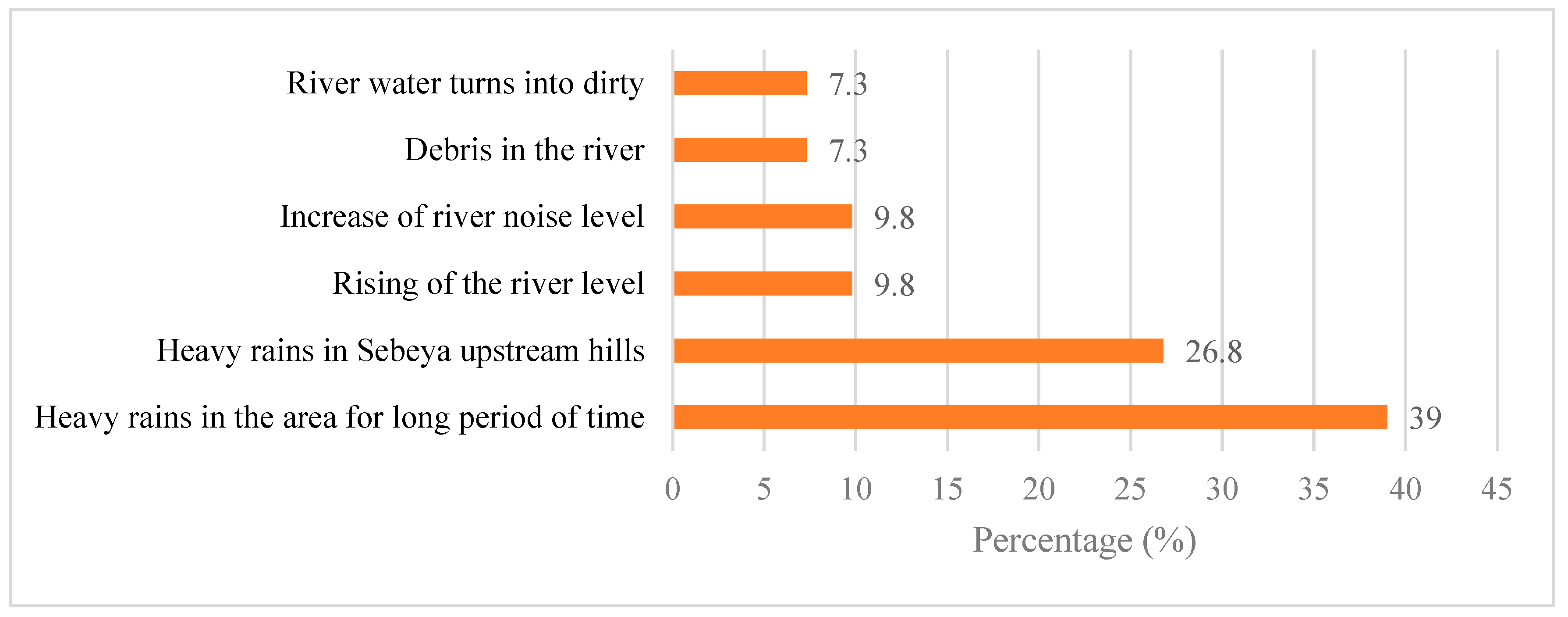
The Figure 8 presents the key indicators of flooding in the Sebeya Catchment, highlighting the most common warning signs observed by local communities. The dominant indicator is heavy rains in the area for an extended period, which accounts for 39% of reported signs. It suggests that prolonged rainfall is the primary trigger of floods in the region, leading to excessive surface runoff and water accumulation. Different studies confirmed that rainfall is the main indicator of flooding [50]. Additionally, heavy rains in the upstream hills of Sebeya contribute 26.8%, indicating that even if rainfall is not directly experienced in lower areas, runoff from elevated regions significantly influences flood risks. These findings emphasize the strong relationship between precipitation and flooding in the catchment.
Other notable flood indicators include the rising of river levels (9.8%) and the increase in river noise levels (9.8%), both of which serve as immediate signs of an impending flood. Changes in river characteristics, such as the presence of debris (7.3%) and turbidity (7.3%), are also critical warnings that flooding may occur. These physical changes suggest increased water velocity and erosion, which often precede overflow events. The distribution of these indicators highlights the importance of community awareness and early warning systems based on observable environmental changes. By recognizing these signs, residents can take preventive measures to reduce flood-related damage.
Figure 8.
indicative signs of observed flood in the Sebeya catchment.
3.5.2. Impact of Flood on Livelihood
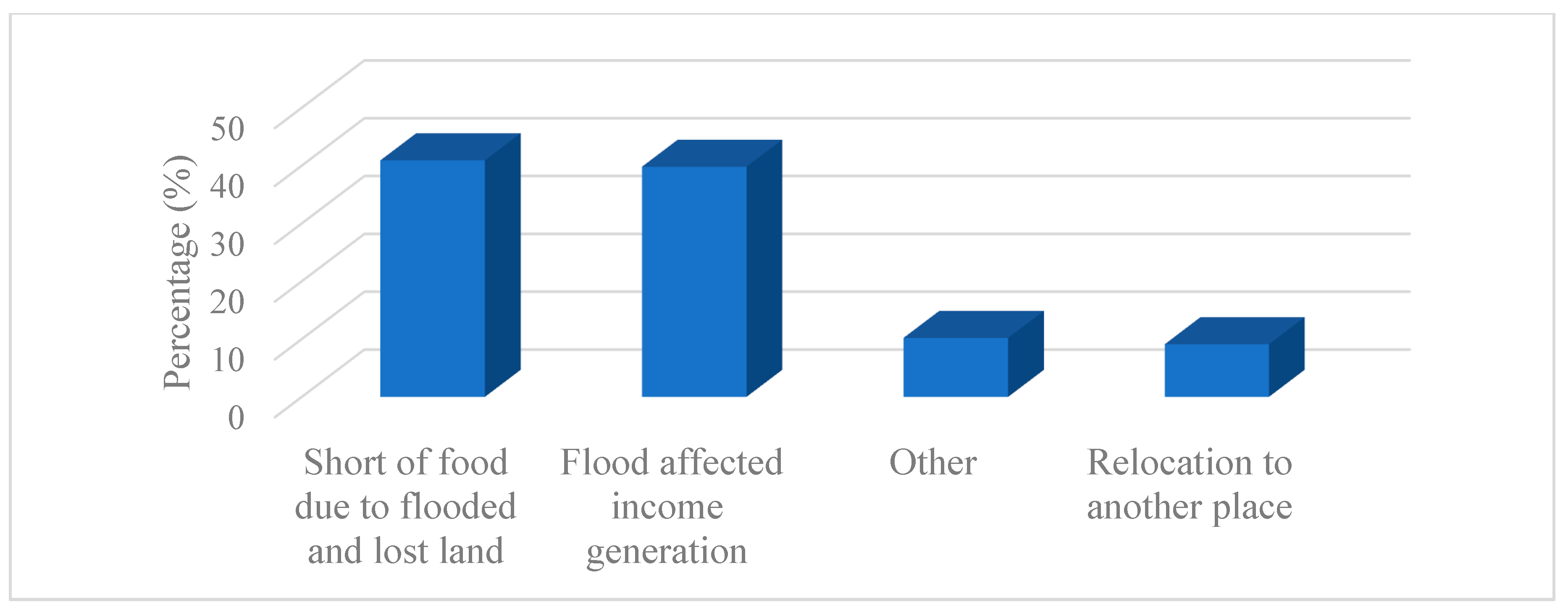
In the current study we assessed the respondents’ views on the impacts of flood on their health; the Figure 9 highlights the significant floods impact on livelihoods within affected region. Most prominent consequence is food shortages due to flooded and lost agricultural land, affecting 40.9% of people. It indicates that agriculture, a significant source of food and income, is highly vulnerable to flooding, leading to food insecurity. Additionally, 39.8% of respondents reported that flooding affected their income generation, showing that not only farmers but also other workers relying on local businesses, trade, and services are financially impacted. 10.2% of the population experienced other effects, which could include health issues, infrastructure damage, and disrupted education. Lastly, 9.1% of the affected individuals had to relocate due to severe flood conditions, indicating displacement and loss of homes. These findings underscore the urgent need for flood mitigation measures to protect livelihoods, ensure the food security, and support economic resilience in flood-susceptible areas.
Figure 9.
Impacts of flooding on livelihoods in the Sebeya catchment.
3.5.3. Flood Impact on Livelihoods
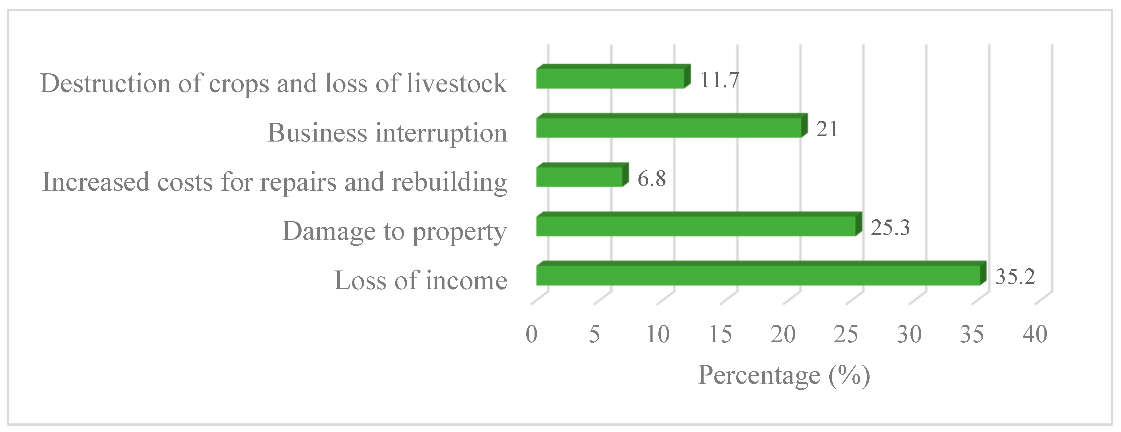
Figure 10 indicates that the economic flood impacts within Sebeya catchment are severe, affecting multiple sectors, with loss of income (35.2%) being the most significant consequence. It highlights how floods disrupt livelihoods, especially for those dependent on agriculture, small businesses, and daily wages. Many people lose employment opportunities due to damaged workplaces and infrastructure, reducing household earnings and increasing financial insecurity. Additionally, business interruption (21.0%) further worsens the situation, as markets, shops, and enterprises are forced to close temporarily or permanently due to water damage, supply chain disruptions, and reduced customer access. These economic setbacks create long-term challenges, delaying recovery and limiting community resilience against future floods.
Beside direct income loss, flooding leads to property damage (25.3%), increased costs for repairs and rebuilding (6.8%), as well as placing a heavy financial burden on affected households and businesses. Homes, shops, roads, and other infrastructure suffered extensive destruction, requiring significant investments for reconstruction. Furthermore, the destruction of crops and loss of livestock (11.7%) weakens food security and the agricultural economy, reducing farm productivity and escalating food prices. These combined economic impacts underscore the urgent need for proactive flood mitigation strategies, such as flood-resistant infrastructure, improved drainage systems, and financial support mechanisms like insurance and emergency relief programs to help communities recover and build resilience. Various studies have demonstrated the flood economic impacts in different regions around the world [51], [52].
Figure 10.
Economic impacts of flooding on livelihoods in the Sebeya catchment.
3.5.4. Impacts of Flooding on Agriculture Activities
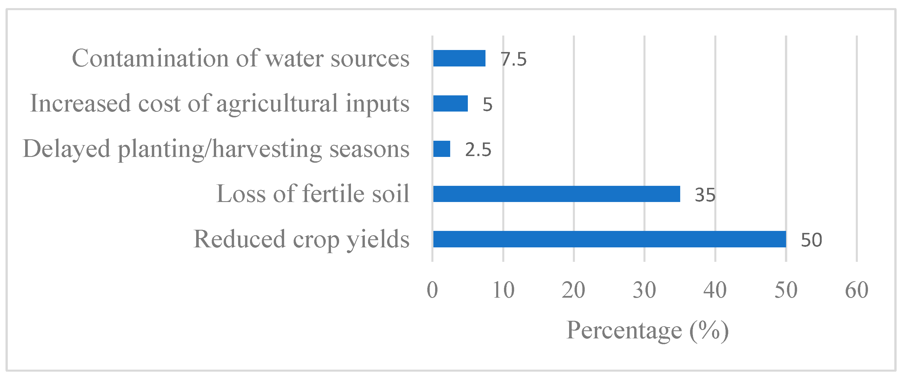
Figure 11 highlights that flooding has a devastating impact on agricultural activities in the Sebeya Catchment, with reduced crop yields (50.0%) being the most significant consequence. It indicates that prolonged waterlogging, soil erosion, and crop destruction severely affect food production, leading to food insecurity and economic instability for farmers. Additionally, the loss of fertile soil (35.0%) further worsens agricultural productivity, as floods wash away nutrient-rich topsoil essential for crop growth. Without proper soil conservation measures, the long-term viability of farming in the region is threatened, requiring farmers to invest in soil restoration efforts such as terracing and reforestation to mitigate further losses.
Other impacts of flooding on agriculture, though less prominent, still contribute to production challenges. Contamination of water sources (7.5%) poses a serious risk, as polluted irrigation water can damage crops and spread plant diseases, reducing overall yields. Additionally, increased cost of agricultural inputs (5.0%) burdens farmers to purchase fertilizers, pesticides, and improved seeds to restore productivity. Delayed planting and harvesting seasons (2.5%) also contribute to instability, as unpredictable weather patterns disrupt traditional farming cycles. These findings show-up the urgent need for improved flood mitigation measures, such as sustainable land-use planning, better drainage infrastructure, and farmer support programs, to protect agricultural livelihoods in the Sebeya Catchment.
Figure 11.
Impacts of flooding on agricultural activities in the Sebeya catchment.
3.5.5. Impacts of Flooding on Access to Essential Services
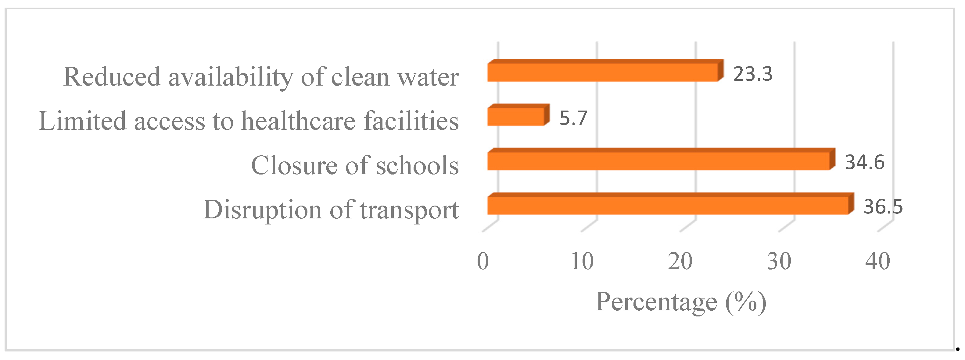
Flooding significantly disrupts access to essential services in the Sebeya Catchment (Figure 12), with transportation disruptions (36.5%) being the most affected sector. Flooded roads and damaged bridges hinder movement, temporarily preventing residents to reach markets, workplaces, and emergent assistance. Similarly, school closures (34.6%) pose a significant challenge, as flooded schools and impassable roads prevent students from attending classes, leading to learning disruptions. Additionally, the reduced availability of clean water (23.3%) highlights a critical health risk, as floods contaminate water sources, increasing the spread of waterborne diseases. Limited access to healthcare facilities (5.7%) further exacerbates the situation, as damaged infrastructure and transportation barriers prevent timely medical assistance. These impacts emphasize the need for resilient infrastructure, emergency response systems, and long-term flood mitigation measures to ensure continuous access to essential services.
Figure 12.
Impacts of flooding on access to essential services in the Sebeya catchment.
3.5.6. Impacts of Flooding on Infrastructure
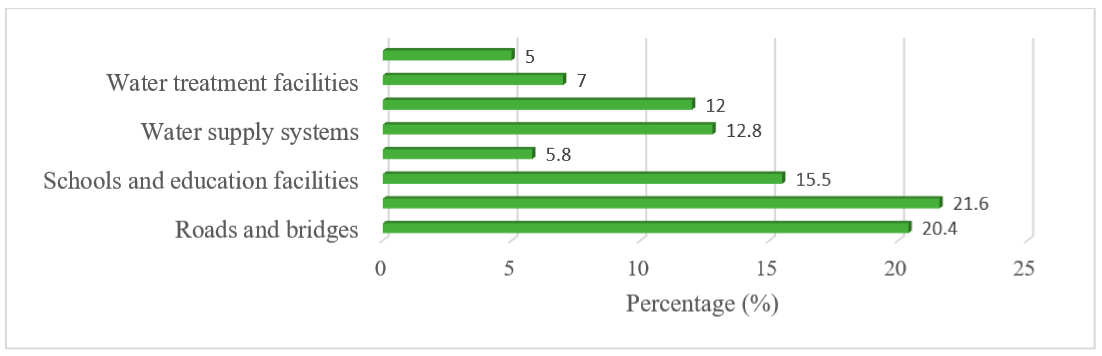
As mentioned in Figure 13, the results showed that flooding has a widespread impact on infrastructure in the Sebeya Catchment, with residential and commercial buildings (21.6%) and roads and bridges (20.4%) being the most affected. Floodwaters weaken the foundations of buildings, causing structural damage and, in some cases, destruction, leaving families and businesses displaced. The disruption of roads and bridges severely affects transportation, hindering the movement of people, goods, and emergency response teams. It not only isolates communities but also slows economic activities, making recovery efforts more difficult. Similarly, schools and education facilities (15.5%) suffer damage, leading to prolonged closures and negatively affecting students’ learning opportunities.
Other essential infrastructure systems are also significantly impacted. Water supply systems (12.8%) and electrical power lines (12.0%) are highly vulnerable, with floods contaminating clean water sources and damaging power networks, resulting in water shortages and electricity blackouts. Water treatment facilities (7.0%) also face operational challenges, increasing the risk of waterborne diseases. The damage to healthcare facilities (5.8%) further compounds the crisis, as limited medical services reduce the community’s ability to respond to injuries and disease outbreaks. These impacts highlight the urgent need for climate-resilient infrastructure, improved drainage systems, and investment in flood-resistant building designs to minimize future flood-related disruptions.
Figure 13.
Impacts of flooding on infrastructure in the Sebeya catchment.
4. Discussion
This study has considered nine (9) factors for mapping of flood susceptibility in Sebeya catchment. These factors intervened separately, and to differing degrees where each factor was thus separated into five classes, to which ratings were given based on the class's level of influence.
4.1. Elevation
Elevation is crucial in determining flood susceptibility, as lower-lying areas are naturally more vulnerable to flooding compared to higher-elevation areas.Regions at or below sea level, near rivers or floodplains, are particularly vulnerable because they lack sufficient drainage and are quickly inundated during heavy rainfall, storm surges, or dam failures [53]. Conversely, higher elevations generally experience less flooding as water flows downhill, reducing the likelihood of standing water accumulation. However, steep slopes can also lead to flash floods when excessive rainfall runs off quickly, eroding soil and overwhelming drainage systems[54]. Additionally, urban development in low-lying areas often involves deforestation and paving over natural drainage areas, increasing run-off and decreasing the absorption capacity of the land. Deforestation and improper land use in mountain regions can make slopes more susceptible to rapid runoff. The Sebeya catchment is situated on rocky terrain, with elevations ranging from 1486 to 2979 meters, and average elevation of 2293 meters. The elevation map of the area shown in Figure 5(a) has been split into five (5) classes 1486 – 1831 m, 1831 – 2071m, 2071 – 2306 m, 2306 – 2551m, and 2551 – 2979 m.
4.2. Slope
Slope or land inclination is the proportion of the horizontal distance (length of the flat land) to the vertical distance (elevation of the land). Flood disaster risk increases with slope inclination; on the other hand, flood disaster risk decreases with slope steepness[55]. Slope significantly influences flood susceptibility by affecting how water moves across the land. In areas with steep slopes, water runs off quickly, minimize chances of prolonged floods but accentuate flash floods risk. These fast-moving waters can carry debris, erode soil, and overwhelm drainage systems, leading to sudden and destructive flooding. Conversely, flatter areas retain water longer, making them more susceptible to standing water and prolonged inundation [56]. The slope parameter for Sebeya catchment is derived from DEM data and is categorized into five levels using the classification of natural breaks. These levels encompass very low (0.0 – 11.0%), Low (11.0 – 22.0%), Moderate (22.0 – 33.0%), High (33.0 – 46.0%), and Very high (46.0 – 87.0%) Figure 5(b).
4.3. Topographic Wetness Index
The Topographic Wetness Index (TWI) is a key hydrological parameter influencing flood susceptibility by indicating areas prone to water accumulation [57]. TWI is calculated using slope and upstream contributing area, with higher values representing areas in which water has possibility to pool, such as valleys, floodplains, and depressions [58]. These high-TWI areas tend to have lower drainage efficiency, causing them to be exposed to prolonged inundation during intense rains. Conversely, regions with low TWI values, such as steep slopes and ridges, promote rapid runoff, reducing standing water but increasing the potential for flash floods downstream. The TWI map presented in Figure 5(c) is split into five categories with the values which range from -6.86 - -4.91, -4.91 - -3.23, -3.23 - -0.87, -0.87 - 2.36, and 2.36 - 10.30.
4.3. Land Use/ Land Cover
Land cover has an important role in floods susceptibility by affecting how water is absorbed, stored, and drained across different surfaces. Natural vegetation, such as forests and wetlands, helps mitigate flooding by enhancing infiltration, reducing surface runoff, and promoting groundwater recharge[59]. In contrast, impervious surfaces like concrete, asphalt, and compacted soil in urban areas prevent water from being absorbed into the ground, leading to increased runoff and a higher risk of urban flooding [60]. Human-induced land cover changes further exacerbate flood susceptibility. Deforestation removes critical vegetation that stabilizes soil and slows water movement, increasing the likelihood of flash floods and landslides [59]. The landuse/land cover map of the Sebeya catchment is shown in Figure 5(d). It is split into five categories including Water body, Agriculture, Settlement, Barren Land, and Vegetation.
4.5. Normalized Vegetative Index
The Normalized Difference Vegetation Index (NDVI) is a key indicator of vegetation health and density, significantly influencing flood susceptibility [61]. Areas with high NDVI values, indicating dense and healthy vegetation, tend to experience lower flood risks because vegetation enhances soil infiltration, stabilizes slopes, and reduces surface runoff. Forests, grasslands, and wetlands with high NDVI absorb excess water, acting as natural flood buffers. Conversely, areas with low NDVI values, such as barren land, urban environments, or deforested regions, have reduced water absorption capacity, leading to increased runoff and high flood likelihood, especially during intense rainfall. Changes in NDVI over time can also serve as an early warning sign of increasing flood susceptibility. Deforestation, urban expansion, and land degradation lower NDVI values reducing the land’s ability to retain water and increasing the risk of flash floods and erosion. In the Sebeya catchment deforestation, agricultural expansion, and land degradation in the catchment contribute to lower NDVI values, increasing the risk of floods, and it is ranging from 0.007 - 0.192, 0.192 - 0.256, 0.256 - 0.309, 0.309 - 0.364, and 0.364 - 0.713.
4.6. Precipitation
Precipitation is among the most significant factors associated with flood susceptibility, as the amount, intensity, and duration of rainfall directly determine the likelihood of flooding [62]. Heavy and prolonged rainfall can saturate the soil, reducing its ability to absorb water and producing excess runoff. This runoff accumulates in rivers, lakes, and low-lying areas, increasing the risk of flooding. Intense, short-duration rainfall, during thunderstorms or tropical storms, can overwhelm drainage systems and cause flash floods, especially in urban areas with impervious surfaces. Additionally, heavy precipitation can trigger landslides and debris flows in regions with steep terrain, further exacerbating flood risks.
Seasonal and climatic patterns also influence the impact of precipitation on flooding. Monsoons, hurricanes, and El Niño events can bring excessive rainfall, increasing flood susceptibility in affected regions. Climate change intensifies precipitation extremes, making storms more frequent and severe, thereby heightening global flood risks. Furthermore, snowmelt from the high-altitude areas during warm seasons can contribute to river flooding when combined with rainfall. Effective flood risk management requires accurate precipitation forecasting, improved drainage infrastructure, and sustainable land management strategies to mitigate the effects of extreme rainfall events. The rainfall distribution map in the Sebeya catchment subdivided into 5 categories ranging from 1188 – 1286 mm, 1286 – 1333 mm, 1333 – 1378 mm, 1378 – 1438 mm, and 1438 – 1537 Figure 5(e), with an average rainfall of 1325 mm, which is significantly high.
4.7. Drainage Density
Drainage density, defined as the total length of streams and rivers per unit area, plays a critical role in flood susceptibility by determining how efficiently a landscape can transport excess water [63]. Areas with high drainage density have numerous water channels that can quickly convey runoff, reducing the likelihood of prolonged flooding. However, if these channels become overwhelmed due to extreme rainfall or poor maintenance, the risk of flash floods increases. In contrast, regions with low drainage density have fewer natural outlets for water, leading to slower drainage and a higher potential for water accumulation, especially in flat or poorly permeable landscapes. Figure 5(f) displays the Sebeya catchment's drainage density map, which has been categorized into five classes with values ranging from 0 to 795 km/km². At confluences and along watercourses, their values are elevated. A rating of 10 has been given to the density classes because of their substantial role in the flooding process (Table 2).
4.8. Distance from the River
The distance from a river mostly influences flood susceptibility [64], as areas closer to rivers are more prone to flooding due to their proximity. Floodplains, which are low-lying areas adjacent to rivers, are especially vulnerable because they naturally serve as overflow regions when rivers exceed their banks. During extreme weather events, such as hurricanes or prolonged rainfall, these areas experience high flood risks due to rapid water accumulation. Conversely, locations farther from rivers generally face lower flood risks, as they are less directly affected by river overflow. However, poor drainage and heavy rainfall can cause localized flooding even in distant areas. Human activities can modify how distance from a river affects flood susceptibility. Urban expansion into floodplains increases exposure to flooding, especially when natural buffers like wetlands are removed. Levees and dams can provide temporary flood protection but may fail under extreme conditions, leading to catastrophic flooding in nearby areas [65].
The distance from the river map in Sebeya catchment falls into five major classes: 0–102 m, 102–210 m, 210–310 m, 310–431 m, and 431–815 m (Figure A.2f). Given its significant risk of flooding, the distance from the river class with the lowest values (0–102 m) receives a score of 10. Those that are farthest from the river (431–815 m) experience the reverse outcome. According to Table 2, the latter class has been given a rating of 1.
4.9. Distance from Road
The distance from roads can influence flood susceptibility due to how roads alter natural water flow and drainage patterns [66]. Roads, especially those with impermeable surfaces like concrete and asphalt prevent water infiltration, which causes increased surface run-off. Areas near roads with inadequate drainage systems are more prone to flooding, as water can accumulate rapidly, overwhelming storm drains and creating localized floods. Additionally, roads built on elevated embankments can act as barriers, obstructing natural water pathways and causing water to pool in adjacent low-lying areas. In contrast, areas farther from roads may experience less direct runoff impact, though they can still be affected by poor regional drainage or redirected water flow. In the current study, distance from road ranging from 0 – 327 m, 327 – 854 m, 854 – 1453 m, 1453 – 2151m, and 2151 – 3632m. The lower the distance indicates high probability of susceptible to flood.
4.10. Flood Susceptibility and Policy Implication Nexus in Sebeya Catchment
Flood susceptibility mapping in Sebeya catchment shows important spatial patterns of various zones sensitive to floods, and this has significant implications for land-use planning, environmental management, and disaster risk reduction policy not only in Rwanda but also in neighboring countries located in East Africa rift valley. The identification of flood susceptible zones along Sebeya River and its tributaries, low-lying floodplains, and rapidly populated areas in Sebeya highlights the urgent need for stricter policy development in vulnerable areas. Local and national authorities can use these findings to avoid informal settlements in high-risk regions, enforce building setbacks from riverbanks, and advise zoning restrictions. Additionally, the flood susceptibility map provides an empirical basis for integrating flood risk considerations into environmental impact assessments and strategic urban development plans within the Sebeya catchment, thereby promoting more resilient and sustainable land-use practices.
In addition to spatial planning, the findings have significant implication for infrastructure development, disaster preparedness, and climate adaptation policies. The identification of flood hotspots facilitates the prioritization of both structural and non-structural mitigation strategies, including the development of drainage upgrades, river training projects, wetland restoration, and the installation of early warning systems in areas that are particularly vulnerable. By concentrating investments on the most vulnerable sectors and communities, policymakers can maximize the distribution of scarce resources. Given the anticipated escalation of extreme rainfall events, the flood susceptibility assessment further emphasizes the necessity of integrating climate change adaptation into water resources and disaster management policy. Furthermore, flood susceptibility mapping is an essential decision-support tool for enhancing flood governance, community readiness, and long-term resilience in the Sebeya catchment since it offers a scientifically based risk information framework.
5. Conclusions
Flood susceptibility mapping in the Sebeya Catchment is a crucial tool for understanding and mitigating the risks associated with frequent flooding events. Nine flood associated factors were analyzed through GIS-AHP approaches. Additionally, a survey was conducted to assess socio-economic impacts of flood in the study area. The analysis of hydrological and topographic parameters identified rainfall, elevation, slope, and drainage density as major determinants of flood susceptibility. The flood susceptibility mapping has indicated that 25.7%, 46.5%, and 27.8% of the catchment are located in high, moderate, and low susceptible zones respectively. The results suggest that flooding disproportionately affects agricultural livelihoods and infrastructure, underscoring the socio-economic vulnerability of communities in low-lying zones of the study area. Flooding also presents health and environmental risks, with contaminated water sources leading to outbreaks of waterborne diseases such as cholera and dysentery within the displaced families facing poor sanitation facilities. It is therefore crucial to mitigate flood risks and minimize socio-economic impacts by implementing an integrated flood management strategy in the Sebeya Catchment. Structural measures such as the construction of flood control infrastructures, including levees, retention basins, and improved drainage systems, should be prioritized. In addition, reforestation and afforestation programs should be encouraged to enhance soil stability and reduce surface runoff for sustainable land-use planning. Non-structural measures, such as community awareness programs and early warning systems, should be strengthened to improve disaster preparedness and response. Investing in hydrological monitoring systems and real-time flood forecasting tools can help authorities provide timely alerts, reducing casualties and property damage. Additionally, the government should establish financial support mechanisms, such as insurance programs and emergency relief funds, to assist flood-affected households. By integrating these recommendations, the Sebeya catchment can build resilience against flooding, safeguarding both its people and economic stability. Further studies should develop the economic losses prediction model based on flood susceptibility mapping
Author Contributions
A.M., T.K., F.M., and L.M. contributed to the conception. Conceptualization, supervision, and review were contributed by T.K., F.M. and L.M. Data collection and analysis were contributed by A.M. Original draft writing was performed by A.M. All authors have read and agreed to the published version of the manuscript.
Funding
This research didn’t receive any fund.
Institutional Review Board Statement
Not applicable.
Informed Consent Statement
Not applicable.
Data Availability Statement
The data supporting the findings of this study are available from the corresponding author upon request.
Acknowledgments
We thank the Rubavu district to facilitate during community’s survey.
Declaration of conflict of interest
The authors declare that they have no conflict of interest.
References
- M. Tanoue, R. Taguchi, H. Alifu, and Y. Hirabayashi, “Residual flood damage under intensive adaptation,” Nat. Clim. Chang., vol. 11, no. 10, pp. 823–826, 2021. [CrossRef]
- J. Lee, D. Perera, T. Glickman, and L. Taing, “Water-related disasters and their health impacts: A global review,” Prog. Disaster Sci., vol. 8, p. 100123, 2020. [CrossRef]
- J. Rentschler and M. Salhab, “People in Harm’s Way : Flood Exposure and Poverty in 189 Countries.Policy Research Working Paper;No. 9447.,” Poverty Shar. Prosper., vol. 9447, no. 10, p. Policy Working Paper, 2020, [Online]. Available: https://openknowledge.worldbank.org/handle/10986/34655.
- F. Aziz, X. Wang, M. Q. Mahmood, M. Awais, and B. Trenouth, “Coastal urban flood risk management: Challenges and opportunities − A systematic review,” J. Hydrol., vol. 645, no. PB, p. 132271, 2024. [CrossRef]
- Y. B. Kurata, A. K. S. Ong, R. Y. B. Ang, J. K. F. Angeles, B. D. C. Bornilla, and J. L. P. Fabia, “Factors Affecting Flood Disaster Preparedness and Mitigation in Flood-Prone Areas in the Philippines: An Integration of Protection Motivation Theory and Theory of Planned Behavior,” Sustain., vol. 15, no. 8, 2023. [CrossRef]
- D. Aryal et al., “A model-based flood hazard mapping on the southern slope of Himalaya,” Water (Switzerland), vol. 12, no. 2, 2020. [CrossRef]
- M. Vojtek et al., “Comparison of multi-criteria-analytical hierarchy process and machine learning-boosted tree models for regional flood susceptibility mapping: a case study from Slovakia,” Geomatics, Nat. Hazards Risk, vol. 12, no. 1, pp. 1153–1180, 2021. [CrossRef]
- N. K. Mohammadi and N. K. Mohammadi, “Floods Impacts on the Socio-Economic of Livelihoods in Paktia Afghanistan,” Int. J. Res. Appl. Sci. Biotechnol., vol. 8, no. 4, 2021. [CrossRef]
- UNISDR, “Words into Action Guidelines Disaster Displacement : How to Reduce Risk , Address Impacts and Strengthen Resilience A companion for implementing,” p. 70, 2018.
- J. D. Acosta-España, D. Romero-Alvarez, C. Luna, and A. J. Rodriguez-Morales, “Infectious disease outbreaks in the wake of natural flood disasters: global patterns and local implications,” Infez. Med., vol. 32, no. 4, pp. 451–462, 2024. [CrossRef]
- F. Suhr and J. I. Steinert, “Epidemiology of floods in sub-Saharan Africa: a systematic review of health outcomes,” BMC Public Health, vol. 22, no. 1, pp. 1–15, 2022. [CrossRef]
- S. I. I. Kofi Yeboah, P. Antwi-Agyei, A. T. Kabo-Bah, and N. O. Bonsu Ackerson, “Water, environment, and health nexus: understanding the risk factors for waterborne diseases in communities along the Tano River Basin, Ghana,” J. Water Health, vol. 22, no. 8, pp. 1556–1577, 2024. [CrossRef]
- S. A. Shah and S. Ai, “Flood susceptibility mapping contributes to disaster risk reduction: A case study in Sindh, Pakistan,” Int. J. Disaster Risk Reduct., vol. 108, no. April, 2024. [CrossRef]
- C. M. Kaya and L. Derin, “Parameters and methods used in flood susceptibility mapping: a review,” J. Water Clim. Chang., vol. 14, no. 6, pp. 1935–1960, 2023. [CrossRef]
- B. A. Bedada and W. T. Dibaba, “Geoinformatics and AHP multi criteria decision making integrated flood hazard zone mapping over Modjo catchment, Awash river basin, central Ethiopia,” Discov. Appl. Sci., vol. 7, no. 4, 2025. [CrossRef]
- M. Yılmaz and K. D. Alemdar, “Mapping and assessment of flood risk based on vulnerability and hazard factors in urban areas through the integration of multi-criteria techniques and GIS: A case study in Yakutiye, Erzurum, Türkiye,” Environ. Earth Sci., vol. 84, no. 15, pp. 1–22, 2025. [CrossRef]
- R. Bunmi Mudashiru, N. Sabtu, R. Abdullah, A. Saleh, and I. Abustan, “Optimality of flood influencing factors for flood hazard mapping: An evaluation of two multi-criteria decision-making methods,” J. Hydrol., vol. 612, no. September, pp. 1–9, 2022. [CrossRef]
- S. Shrestha, D. Dahal, B. Poudel, M. Banjara, and A. Kalra, “Flood Susceptibility Analysis with Integrated Geographic Information System and Analytical Hierarchy Process : A Multi-Criteria Framework for Risk Assessment and Mitigation,” 2025.
- R. W. Saaty, “The analytic hierarchy process-what it is and how it is used,” Math. Model., vol. 9, no. 3–5, pp. 161–176, 1987. [CrossRef]
- J. G. Gacu, C. E. F. Monjardin, D. B. Senoro, and F. J. Tan, “Flood Risk Assessment Using GIS-Based Analytical Hierarchy Process in the Municipality of Odiongan, Romblon, Philippines,” Appl. Sci., vol. 12, no. 19, 2022. [CrossRef]
- A. B. Ayele, A. Legesse, A. Uncha, and A. Gelaw, “Flood hazard vulnerability assessment in the Sile-Sago watershed, Rift Valley Basin, Ethiopia,” Sci. African, vol. 29, no. March, p. e02846, 2025. [CrossRef]
- A. Mulu, S. B. Kassa, M. Lakew, and T. M. Meshesha, “Flood susceptibility mapping using integrated geospatial and analytical hierarchy process analysis in highly expansive Debre Markos Town, Amhara Region, Ethiopia,” Discov. Appl. Sci., vol. 7, no. 8, 2025. [CrossRef]
- M. Zhran et al., “Exploring a GIS-based analytic hierarchy process for spatial flood risk assessment in Egypt: a case study of the Damietta branch,” Environ. Sci. Eur., vol. 36, no. 1, 2024. [CrossRef]
- D. Diriba, T. Takele, S. Karuppannan, and M. Husein, “Flood hazard analysis and risk assessment using remote sensing, GIS, and AHP techniques: a case study of the Gidabo Watershed, main Ethiopian Rift, Ethiopia,” Geomatics, Nat. Hazards Risk, vol. 15, no. 1, p., 2024. [CrossRef]
- A. Aichi et al., “Integrated GIS and analytic hierarchy process for flood risk assessment in the Dades Wadi watershed (Central High Atlas, Morocco),” Results Earth Sci., vol. 2, no. February, p. 100019, 2024. [CrossRef]
- G. Parajuli, S. Neupane, S. Kunwar, R. Adhikari, and T. D. Acharya, “A GIS-Based Evacuation Route Planning in Flood-Susceptible Area of Siraha Municipality, Nepal,” ISPRS Int. J. Geo-Information, vol. 12, no. 7, 2023. [CrossRef]
- J. Hahirwabasenga, E. Nilsson, M. Larson, H. Bizimana, U. G. Wali, and M. Persson, “Flooding in Sebeya catchment, Rwanda - A review of causes, impacts, and management,” Int. J. Disaster Risk Reduct., vol. 114, no. November, p. 105012, 2024. [CrossRef]
- “Disaster risk mitigation plan for cenr sector,” no. December, 2024.
- IFRC, “Operational Update:Rwanda - Floods and Landslides,” Unhcr, no. December, pp. 1–12, 2023.
- S. Ashfaq, M. Tufail, A. Niaz, S. Muhammad, H. Alzahrani, and A. Tariq, “Flood susceptibility assessment and mapping using GIS-based analytical hierarchy process and frequency ratio models,” Glob. Planet. Change, vol. 251, no. February, p. 104831, 2025. [CrossRef]
- M. Saleh, “Evaluation of Jenks Natural Breaks Clustering Algorithm for Changepoint Identification in Streaming Sensor Data,” IEEE Sensors Lett., vol. 8, no. 10, 2024. [CrossRef]
- J. Chen, S. Yang, H. Li, B. Zhang, and J. Lv, “Research on geographical environment unit division based on the method of natural breaks (Jenks),” Int. Arch. Photogramm. Remote Sens. Spat. Inf. Sci. - ISPRS Arch., vol. 40, no. 4W3, pp. 47–50, 2013. [CrossRef]
- R. Gui, W. Song, X. Pu, Y. Lu, C. Liu, and L. Chen, “A River Channel Extraction Method Based on a Digital Elevation Model Retrieved from Satellite Imagery,” Water (Switzerland), vol. 14, no. 15, pp. 1–16, 2022. [CrossRef]
- K. J. Beven and M. J. Kirkby, “A physically based, variable contributing area model of basin hydrology,” Hydrol. Sci. Bull., vol. 24, no. 1, pp. 43–69, 1979. [CrossRef]
- D. Nsangou et al., “Urban flood susceptibility modelling using AHP and GIS approach: case of the Mfoundi watershed at Yaoundé in the South-Cameroon plateau,” Sci. African, vol. 15, p. e01043, 2022. [CrossRef]
- M. A. Weday, K. W. Tabor, and D. O. Gemeda, “Flood hazards and risk mapping using geospatial technologies in Jimma City, southwestern Ethiopia,” Heliyon, vol. 9, no. 4, p. e14617, 2023. [CrossRef]
- M. S. Siddik, S. S. Tulip, A. Rahman, M. N. Islam, A. T. Haghighi, and S. M. T. Mustafa, “The impact of land use and land cover change on groundwater recharge in northwestern Bangladesh,” J. Environ. Manage., vol. 315, no. October 2021, p. 115130, 2022. [CrossRef]
- R. M. M. Abdusamea, “The Importance of the Normalized Difference Vegetation Index (NDVI) and the Use of the ArcGIS to create NDVI Maps,”, no. 57, pp. 1–7, 2024. [CrossRef]
- K. C. Swain, C. Singha, and L. Nayak, “Flood susceptibility mapping through the GIS-AHP technique using the cloud,” ISPRS Int. J. Geo-Information, vol. 9, no. 12, 2020. [CrossRef]
- R. Wang, Y. Hong, Y. Zhou, Y. He, and D. Andrew, “The influence of road network topology on street flooding in New York City — A social media data approach,” vol. 638, no. July, pp. 1–9, 2024.
- S. Y. Yang, C. H. Chang, C. T. Hsu, and S. J. Wu, “Variation of uncertainty of drainage density in flood hazard mapping assessment with coupled 1D–2D hydrodynamics model,” Nat. Hazards, vol. 111, no. 3, pp. 2297–2315, 2022. [CrossRef]
- K. Seejata, A. Yodying, T. Wongthadam, N. Mahavik, and S. Tantanee, “Assessment of flood hazard areas using Analytical Hierarchy Process over the Lower Yom Basin, Sukhothai Province,” Procedia Eng., vol. 212, no. September 2020, pp. 340–347, 2018. [CrossRef]
- V. Mazarakis et al., “Flood-Hazard Assessment in the Messapios River Catchment (Central Evia Island, Greece) by Integrating GIS-Based Multi-Criteria Decision Analysis and Analytic Hierarchy Process,” Land, vol. 14, no. 3, 2025. [CrossRef]
- M. S. Shrestha et al., “The last mile: Flood risk communication for better preparedness in Nepal,” Int. J. Disaster Risk Reduct., vol. 56, no. February, 2021. [CrossRef]
- C. Singha, N. Chakraborty, S. Sahoo, and Q. B. Pham, A novel framework for flood susceptibility assessment using hybrid analytic hierarchy process - based machine learning methods, vol. 121, no. 11. Springer Netherlands, 2025. [CrossRef]
- A. A. Rostami, M. T. Sattari, and H. Apaydin, “Modeling Flood Susceptibility Utilizing Advanced Ensemble Machine Learning Techniques in the Marand Plain,” pp. 1–27, 2025.
- S. Chengu, M. Assen, and E. Gebeyehu, “Multi - criteria decision analysis for flood hazard mapping in the Itang watershed , lower Baro - Akobo Basin , Southwest Ethiopia,” 2025.
- S. Africa, “Mapping pluralistic future flood risk scenarios for informal settlements in the eThekwini metropolitan municipality ,” pp. 20949–20983, 2025.
- E. Modelling, “Urban Flood Risk analysis using the SWAGU- coupled model and a cloud-enhanced fuzzy comprehensive evaluation method,” vol. 189, no. May, pp. 1–8, 2025.
- T. Yu, Q. Ran, H. Pan, J. Li, J. Pan, and S. Ye, “The impacts of rainfall and soil moisture to flood hazards in a humid mountainous catchment: a modeling investigation,” Front. Earth Sci., vol. 11, no. December, pp. 1–12, 2023. [CrossRef]
- D. Svetlana, D. Radovan, and D. Ján, “The Economic Impact of Floods and their Importance in Different Regions of the World with Emphasis on Europe,” Procedia Econ. Financ., vol. 34, no. 15, pp. 649–655, 2015. [CrossRef]
- Z. Manzoor et al., “Floods and flood management and its socio-economic impact on Pakistan: A review of the empirical literature,” Front. Environ. Sci., vol. 10, no. December, pp. 1–14, 2022. [CrossRef]
- U. López-Dóriga and J. A. Jiménez, “Impact of relative sea-level rise on low-lying coastal areas of catalonia, nw mediterranean, spain,” Water (Switzerland), vol. 12, no. 11, 2020. [CrossRef]
- A. A. Firoozi and A. A. Firoozi, “Water erosion processes: Mechanisms, impact, and management strategies,” Results Eng., vol. 24, no. September, p. 103237, 2024. [CrossRef]
- R. R. Rudra and S. K. Sarkar, “Artificial neural network for flood susceptibility mapping in Bangladesh,” Heliyon, vol. 9, no. 6, p. e16459, 2023. [CrossRef]
- V. Ramesh and S. S. Iqbal, “Urban flood susceptibility zonation mapping using evidential belief function, frequency ratio and fuzzy gamma operator models in GIS: a case study of Greater Mumbai, Maharashtra, India,” Geocarto Int., vol. 37, no. 2, pp. 581–606, 2022. [CrossRef]
- D. N. F. Khumaeroh and D. N. Sari, “Application of Analytical Hierarchy Process (AHP) and Geographic Information System (GIS) in flood hazard analysis in the Rawa Pening Sub-Watershed, Indonesia,” IOP Conf. Ser. Earth Environ. Sci., vol. 1314, no. 1, 2024. [CrossRef]
- H. E. Winzeler, P. R. Owens, Q. D. Read, Z. Libohova, A. Ashworth, and T. Sauer, “Topographic Wetness Index as a Proxy for Soil Moisture in a Hillslope Catena: Flow Algorithms and Map Generalization,” Land, vol. 11, no. 11, 2022. [CrossRef]
- S. Sugianto, A. Deli, E. Miswar, M. Rusdi, and M. Irham, “The Effect of Land Use and Land Cover Changes on Flood Occurrence in Teunom Watershed, Aceh Jaya,” Land, vol. 11, no. 8, 2022. [CrossRef]
- W. Sohn, J. H. Kim, M. H. Li, R. D. Brown, and F. H. Jaber, “How does increasing impervious surfaces affect urban flooding in response to climate variability?,” Ecol. Indic., vol. 118, no. April, p. 106774, 2020. [CrossRef]
- T. Islam, E. B. Zeleke, M. Afroz, and A. M. Melesse, “A Systematic Review of Urban Flood Susceptibility Mapping: Remote Sensing, Machine Learning, and Other Modeling Approaches,” Remote Sens., vol. 17, no. 3, 2025. [CrossRef]
- K. Breinl, D. Lun, H. Müller-Thomy, and G. Blöschl, “Understanding the relationship between rainfall and flood probabilities through combined intensity-duration-frequency analysis,” J. Hydrol., vol. 602, no. July, 2021. [CrossRef]
- B. Pallard, A. Castellarin, and A. Montanari, “A look at the links between drainage density and flood statistics,” Hydrol. Earth Syst. Sci., vol. 13, no. 7, pp. 1019–1029, 2009. [CrossRef]
- P. Yariyan et al., “Flood susceptibility mapping using an improved analytic network process with statistical models,” Geomatics, Nat. Hazards Risk, vol. 11, no. 1, pp. 2282–2314, 2020. [CrossRef]
- E. Juan-diego, A. Mendoza, and M. L. Arganis-juárez, “Alteration of Catchments and Rivers , and the Effect on Floods : An Overview of Processes and Restoration Actions,” 2025.
- H. C. Vu, T. N. To, and H. Le, “Impacts of the road on flood inundation in the Tra Khuc–Ve River basin, Vietnam,” Water Policy, vol. 26, no. 12, pp. 1261–1282, 2024. [CrossRef]
Figure 1.
Location of Sebeya catchment on Rwanda map.

Figure 2.
Flow chart of flood susceptibility mapping in this study.
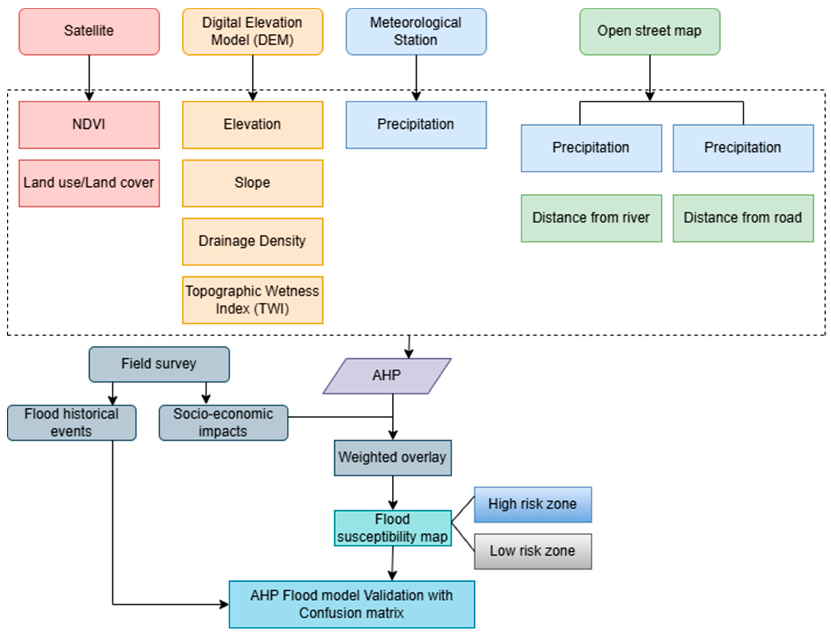
Figure 4.
Flood susceptibility map of the study area.
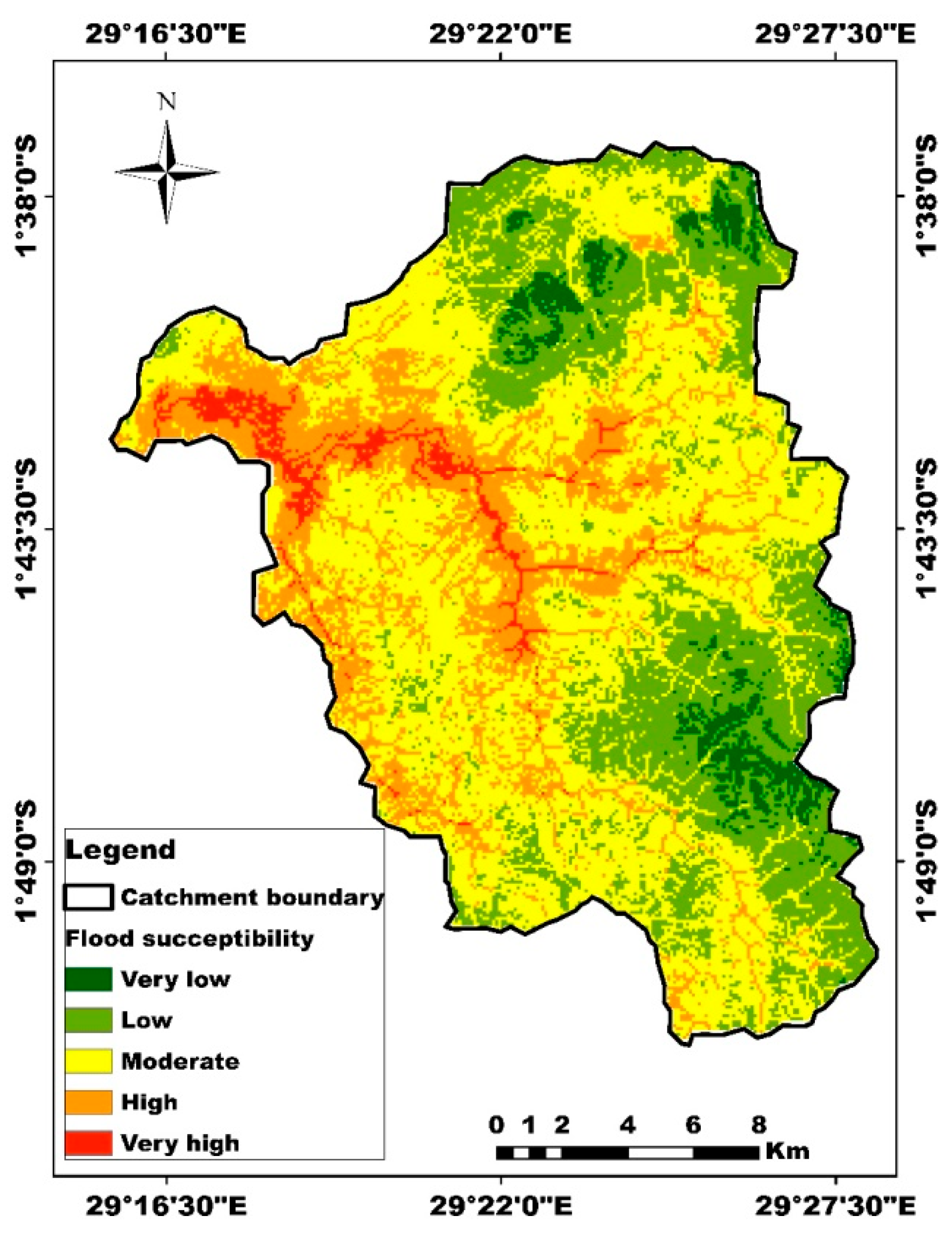
Figure 5.
Socio-economic activities in relation with flood risk.
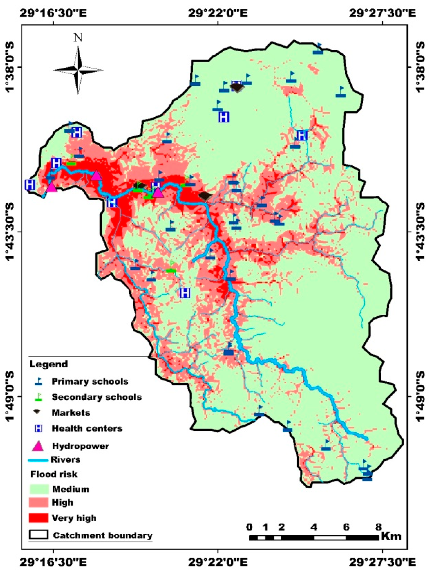

Table 1.
Data sources highlights.
| SN | Type of data | Data category | Acquisition time | Source |
| 1 | Topographical Data (DEM) | Earth data search | 16/12/2024 | https://asf.alaska.edu/asf/asf-services-data-discovery/ |
| 2 | Precipitation (mm/day) | Meteorology data | From 1981 to 2021 | https://www.meteorwanda.gov.rw/index.php?id=30 |
| 3 | Satellite Image | Sentinel-2 (10m) | 02/03/2025 | https://livingatlas.arcgis.com/landcoverexplorer |
| 4 | Road network | Shapefile | 05/03/2025 | https://www.globio.info/download-grip-dataset |
| 5 | River network | Shapefile | 05/03/2025 | https://ihp-wins.unesco.org/dataset/world-rivers |
| 6 | Socio-Economic Data | shapefile | 17/10/2021 | UR-CGIS |
| 7 | Landsat8 image | 30 m | 12/6/2023 | https://earthexplorer.usgs.gov/ |
| 9. | Flood inventory | Points | 21/6/2024 | Flood-prone area in Sebeya |
| 10. | Field survey | N/A | Sebeya catchment |
Table 2.
Criteria and sub-criteria range for flood susceptibility assessment.
| Causal factors | Units | Ranges | Classes | Ratings | Weight (%) |
| TWI | Level | -6.86 - -4.91 | very low | 1 | 13 |
| -4.91 - -3.23 | low | 2 | |||
| -3.23 - -0.87 | moderate | 3 | |||
| -0.87 - 2.36 | high | 4 | |||
| 2.36 - 10.30 | very high | 5 | |||
| Elevation (EL) | m | 1486 - 1831 | very high | 5 | 12 |
| 1831 - 2071 | high | 4 | |||
| 2071 - 2306 | moderate | 3 | |||
| 2306 - 2551 | low | 2 | |||
| 2551 - 2979 | very low | 1 | |||
| Slope(SL) | % | 0 – 11 | very high | 5 | 10 |
| 11 – 22 | high | 4 | |||
| 22 – 33 | moderate | 3 | |||
| 33 – 46 | low | 2 | |||
| 46 – 87 | very low | 1 | |||
| Rainfall/Precipitation (PP) | mm/yr | 1188 - 1286 | very low | 1 | 17 |
| 1286 - 1333 | low | 2 | |||
| 1333 - 1378 | moderate | 3 | |||
| 1378 - 1438 | high | 4 | |||
| 1438 - 1537 | very high | 5 | |||
| Land Use/Land Cover(LULC) | level | Water body | very high | 5 | 7 |
| Agriculture | high | 4 | |||
| Settlement | moderate | 3 | |||
| Barren Land | low | 2 | |||
| Vegetation | very low | 1 | |||
| NDVI | level | 0.007 - 0.192 | very high | 5 | 6 |
| 0.192 - 0.256 | high | 4 | |||
| 0.256 - 0.309 | moderate | 3 | |||
| 0.309 - 0.364 | low | 2 | |||
| 0.364 - 0.713 | very low | 1 | |||
| Distance to river(DRI) | meter | 0 – 573 | very high | 5 | 19 |
| 573 - 1369 | high | 4 | |||
| 1369 - 2465 | moderate | 3 | |||
| 2465 - 3934 | low | 2 | |||
| 3934 - 6350 | very low | 1 | |||
| Distance to road(DRO) | meter | 0 – 327 | very high | 5 | 6 |
| 327 - 854 | high | 4 | |||
| 854 - 1453 | moderate | 3 | |||
| 1453 - 2151 | low | 2 | |||
| 2151 - 3632 | very low | 1 | |||
| Drainage density(DD) | km/km2 | 0 – 47 | very low | 1 | 10 |
| 47 – 143 | low | 2 | |||
| 143 - 265 | moderate | 3 | |||
| 265 - 418 | high | 4 | |||
| 418 - 795 | very high | 5 | |||
| Total | 100 |
Table 3.
Saaty’s 1.0–9.0 scale AHP [19].
Table 3.
Saaty’s 1.0–9.0 scale AHP [19].
| Scales | Importance | Reciprocals |
| 1.0 | Equally important | 1 |
| 3.0 | Moderately important | 1/3 |
| 5.0 | strongly important | 1/5 |
| 7.0 | Very strongly important | 1/7 |
| 9.0 | Extremely important | 1/9 |
| 2.0, 4.0, 6.0, 8.0 | Intermediate values between two factors | 1/2, 1/4, 1/6, 1/8 |
Table 4.
Pair-wise comparison matrix.
| Factors | TWI | EL | SL | PP | LULC | NDVI | DRI | DRO | DD |
| TWI | 1.0 | 1.0 | 1.0 | 1.0 | 2.0 | 2.0 | 1.0 | 5.0 | 1.0 |
| EL | 1.0 | 1.0 | 1.0 | 1.0 | 2.0 | 3.0 | 1.0 | 3.0 | 1.0 |
| SL | 1.0 | 1.0 | 1.0 | 1.0 | 3.0 | 1.0 | 0.5 | 1.0 | 1.0 |
| PP | 1.0 | 1.0 | 1.0 | 1.0 | 3.0 | 2.0 | 2.0 | 3.0 | 1.0 |
| LULC | 0.5 | 0.5 | 0.3 | 0.3 | 1.0 | 1.0 | 0.3 | 3.0 | 1.0 |
| NDVI | 0.5 | 0.3 | 1.0 | 0.5 | 1.0 | 1.0 | 0.2 | 1.0 | 1.0 |
| DRI | 1.0 | 1.0 | 2.0 | 0.5 | 3.0 | 5.0 | 1.0 | 2.0 | 1.0 |
| DRO | 0.2 | 0.3 | 1.0 | 0.3 | 0.3 | 1.0 | 0.5 | 1.0 | 1.0 |
| DD | 1.0 | 1.0 | 1.0 | 1.0 | 1.0 | 1.0 | 1.0 | 1.0 | 1.0 |
| Sum | 7.2 | 7.1 | 9.3 | 6.6 | 16.3 | 17 | 7.5 | 20 | 9 |
Table 5.
Normalized pair-wise comparison matrix.
| Factor | TWI | EL | SL | PP | LULC | NDVI | DRI | DRO | DD | Sum | Criteria weights | Weight (%) |
| TWI | 0.139 | 0.141 | 0.108 | 0.152 | 0.123 | 0.118 | 0.133 | 0.250 | 0.111 | 1.274 | 0.142 | 14 |
| EL | 0.139 | 0.141 | 0.108 | 0.152 | 0.123 | 0.176 | 0.133 | 0.150 | 0.111 | 1.232 | 0.137 | 14 |
| SL | 0.139 | 0.141 | 0.108 | 0.152 | 0.184 | 0.059 | 0.067 | 0.050 | 0.111 | 1.009 | 0.112 | 11 |
| PP | 0.139 | 0.141 | 0.108 | 0.152 | 0.184 | 0.118 | 0.267 | 0.150 | 0.111 | 1.368 | 0.152 | 15 |
| LULC | 0.069 | 0.070 | 0.032 | 0.045 | 0.061 | 0.059 | 0.040 | 0.150 | 0.111 | 0.639 | 0.071 | 7 |
| NDVI | 0.069 | 0.042 | 0.108 | 0.076 | 0.061 | 0.059 | 0.027 | 0.050 | 0.111 | 0.603 | 0.067 | 7 |
| DRI | 0.139 | 0.141 | 0.215 | 0.076 | 0.184 | 0.294 | 0.133 | 0.100 | 0.111 | 1.393 | 0.155 | 15 |
| DRO | 0.028 | 0.042 | 0.108 | 0.045 | 0.018 | 0.059 | 0.067 | 0.050 | 0.111 | 0.528 | 0.059 | 6 |
| DD | 0.139 | 0.141 | 0.108 | 0.152 | 0.061 | 0.059 | 0.133 | 0.050 | 0.111 | 0.953 | 0.106 | 11 |
| Sum | 9.000 | 1.000 | 100 |
Table 6.
Consistency Vector values.
| Factors | TWI | EL | SL | PP | LULC | NDVI | DRI | DRO | DD | CV |
| TWI | 0.142 | 0.137 | 0.112 | 0.152 | 0.142 | 0.134 | 0.155 | 0.293 | 0.106 | 1.373 |
| EL | 0.142 | 0.137 | 0.112 | 0.152 | 0.142 | 0.201 | 0.155 | 0.176 | 0.106 | 1.323 |
| SL | 0.142 | 0.137 | 0.112 | 0.152 | 0.212 | 0.067 | 0.077 | 0.059 | 0.106 | 1.065 |
| PP | 0.142 | 0.137 | 0.112 | 0.152 | 0.212 | 0.134 | 0.31 | 0.176 | 0.106 | 1.481 |
| LULC | 0.071 | 0.069 | 0.034 | 0.046 | 0.071 | 0.067 | 0.046 | 0.176 | 0.106 | 0.685 |
| NDVI | 0.071 | 0.041 | 0.112 | 0.076 | 0.071 | 0.067 | 0.031 | 0.059 | 0.106 | 0.634 |
| DRI | 0.142 | 0.137 | 0.225 | 0.076 | 0.212 | 0.335 | 0.155 | 0.117 | 0.106 | 1.505 |
| DRO | 0.028 | 0.041 | 0.112 | 0.046 | 0.021 | 0.067 | 0.077 | 0.059 | 0.106 | 0.558 |
| DD | 0.142 | 0.137 | 0.112 | 0.152 | 0.071 | 0.067 | 0.155 | 0.059 | 0.106 | 1 |
Table 7.
Consistency and average weight vectors ratio.
| Parameter | Factors | Sum | ||||||||
| TWI | EL | SL | PP | LULC | NDVI | DRI | DRO | DD | ||
| CV | 1.3729 | 1.3226 | 1.0646 | 1.4811 | 0.6849 | 0.6338 | 1.5049 | 0.5577 | 1.0004 | |
| Average Weight | 0.1417 | 0.137 | 0.1123 | 0.1522 | 0.0708 | 0.067 | 0.1548 | 0.0587 | 0.106 | |
| Ratio | 9.691 | 9.6537 | 9.4773 | 9.7299 | 9.6769 | 9.4594 | 9.7229 | 9.5066 | 9.4382 | 86.234 |
Table 9.
Random Index.
| n | 1 | 2 | 3 | 4 | 5 | 6 | 7 | 8 | 9 | 10 |
| RI | 0 | 0 | 0.58 | 0.9 | 1.12 | 1.24 | 1.32 | 1.41 | 1.45 | 1.49 |
Table 10.
Flood susceptibility area coverage and percentage.
| Flood susceptibility | Covered area (km2) | Covered area (%) |
| Very low | 47.64 | 13.1 |
| Low | 108.69 | 29.9 |
| Moderate | 86.62 | 23.9 |
| High | 86.36 | 23.8 |
| Very high | 33.70 | 9.3 |
| Total | 363.01 | 100.0 |
Table 11.
Flood susceptible zones coverage.
| Classification | Area covered ( Km2) | Percentage (%) |
| low | 99 | 27.8 |
| Moderate | 165.6 | 46.5 |
| High | 91.4 | 25.7 |
| Total area | 356 | 100 |
Disclaimer/Publisher’s Note: The statements, opinions and data contained in all publications are solely those of the individual author(s) and contributor(s) and not of MDPI and/or the editor(s). MDPI and/or the editor(s) disclaim responsibility for any injury to people or property resulting from any ideas, methods, instructions or products referred to in the content. |
© 2025 by the authors. Licensee MDPI, Basel, Switzerland. This article is an open access article distributed under the terms and conditions of the Creative Commons Attribution (CC BY) license (http://creativecommons.org/licenses/by/4.0/).
Copyright: This open access article is published under a Creative Commons CC BY 4.0 license, which permit the free download, distribution, and reuse, provided that the author and preprint are cited in any reuse.


