
Submitted:
06 December 2025
Posted:
09 December 2025
You are already at the latest version
Abstract
Growing cooling demand and environmental concerns surrounding mechanical vapour compression systems motivate research into alternative technologies capable of converting low-grade heat into useful cooling. Silica-gel/water single-stage dual-bed adsorption chillers (ADCs) are promising candidates, however, their design must balance conflicting performance targets. This study proposes a regression-assisted multi-objective optimisation framework for low-grade-heat ADC, combining statistically validated surrogate models with the Ant Lion Optimiser and its multi-objective variant. Three co-equal objectives, coefficient of performance (COP), cooling capacity (Q_cc) and waste-heat recovery efficiency (η_e) are jointly maximised to map an operational envelope for sustainable cooling. Two-dimensional Pareto-optimal solutions exhibit a one-dimensional ridge in which η_e declines, and COP and Q_cc increase simultaneously. Within the explored bounds, non-dominated ranges span COP=0.675–0.717, Q_cc=18.3–27.5 kW and η_e=0.118–0.127, with a practical compromise near COP ≈ 0.695, Q_cc ≈ 24 kW and η_(e )≈ 0.122–0.123. While mass flow rate decisions increase Q_cc at the expense of η_e, a one-at-a-time sensitivity analysis with re-optimisation identifies the hot- and chilled-water inlet temperatures and exchanger conductance as the dominant decision variables and maps diminishing-return regions. The proposed framework can effectively use low-grade heat in future low-carbon buildings and processes and supports the configuration of ADC systems.
Keywords:
adsorption chiller
; multi-objective optimisation
; antlion optimiser (ALO)
; multi-objective antlion optimisation (MOALO)
; regression-based surrogate models
; low-grade waste heat
1. Introduction
Recent decades have seen the transition of air conditioners from luxury to an integral part of modern standards of well-being and comfort. Aside from extreme heat-related illnesses like heat stroke, exhaustion and syncope, exposure to extremely low temperatures, particularly among infants and the aged, urbanisation, rising temperatures, and incomes are stoking the global demand for space cooling [1,2,3]. Human activities are gradually contributing to global warming and causing dramatic shifts in energy-use patterns [4]. The energy cost of cooling buildings steadily rises relative to other energy uses [5]. Projections show that 68% of the world's population will live in urban areas by 2050, implying an expansion of air conditioner ownership and electricity use this decade and beyond [6,7]. This emphasises the need to use modern digital tools and decision-support technologies to configure and optimise efficient, sustainable and low-carbon cooling solutions.
Typically, indoor spaces are cooled by electric fans or air conditioners, with air conditioners being the most energy-intensive choice. The most prevalent refrigeration and air conditioning systems are the Mechanical vapour compression (MVC) systems, and they require a substantial amount of high-grade energy to power the compressor and initiate the cooling cycle [8,9]. Additionally, the refrigerants commonly used in MVC systems have been reported to have high ozone depletion potential (ODP) and global warming potential (GWP) and could be very poisonous [10,11].
It has been reported that the cooling of rooms accounts for almost a fifth of the electricity used by buildings. Currently, approximately 135 million air conditioners are sold annually, with projections of even higher sales figures in the coming years [12]. The increased usage of air conditioning has an instantaneous effect on electricity usage. This brings into question the long-term supply and sustainability of electricity resources [13]. Moreover, a 2 - 3% annual growth in electricity demand by 2030 is anticipated by the projections of the expanding world economy [13].
These drawbacks of mechanical vapour compression (MVC) systems have driven research efforts to explore and identify energy-efficient technological cooling alternatives [9]. The adsorption cooling chiller (ADC) represents a promising alternative to the conventional, high-energy-consuming MVC systems. Notably, multi-bed adsorption chillers have shown significant potential as a feasible solution. A key advantage of ADCs is their ability to operate fully or partially by low-grade energy sources like industrial solar, biomass and waste heat for heating and cooling [14]. Also, they use environmentally safe refrigerants with further benefits like durability, quiet functioning, lower energy requirements, and simple controls [15,16]. Thus, ADCs are presented as emerging sustainable cooling technologies that can be used for future low-carbon buildings and industrial operations. While adsorption chillers offer potential advantages, they also have notable limitations. These include suboptimal performance indicators like Specific Cooling Power (SCP), Coefficient of Performance (COP), high manufacturing costs, system complexity and sensitivity to operational parameters such as variations in flow rates, temperature, and working fluids. Addressing these limitations requires a robust research approach to optimise long-term dynamic performance, particularly when powered by waste or renewable heat sources [17].
This study optimises the performance of a single-stage dual-bed ADC, allowing the findings to be potentially extended to complex bed ADCs in the future. Specifically, it develops a framework that acts as a computerised decision-support tool for configuring such ADC systems.
Optimisation techniques such as single and multi-objective optimisation, which use advanced algorithms, can be employed to systematically analyse parametric interactions and serve as sub-models to improve the performance metrics and design criteria of ADCs. Optimisation techniques are computational methods used for finding ideal designs, and multi-objective optimisation specifically handles problems with several objectives, where the inherent conflicting nature of these objectives results in multiple solutions. Consequently, the multi-objective nature of most real-world engineering problems makes them appropriate for multi-objective optimisation applications due to the inherent trade-offs between performance metrics [18,19]. When combined with surrogate models, these techniques form useful digital tools for exploring high-dimensional design spaces and supporting engineering decisions.
Our earlier work on algorithmic optimisation of ADC systems [20] provides a detailed comparative summary of optimisation and control studies for silica-gel/water and multi-bed ADCs. This includes three-bed mass-recovery cycles, periodic optimal control, and integrated design and control frameworks. In this present study, we build on previous research by focusing on a single-stage dual-bed silica-gel/water ADC.
This study introduces as a co-equal objective alongside COP and Qcc rather than a derived metric. As a co-equal to COP and , is used consistently through modelling, single and multi-objective optimisation, plotting, validation with external literature and design guidance. This is to explicitly inform design source utilisation choices and quantify how low-grade heat can be effectively converted to useful cooling. In this way, waste heat recovery efficiency is treated as a core design target as opposed to a secondary indicator.
The structure of this paper is as follows: Section 2 discusses the materials and methods; Section 3 covers the adsorption chiller system optimisation details, along with the Antlion optimisation technique and problem mathematical formulation; and Section 4 discusses the optimisation and sensitivity analysis results.
Thus, this research aims to achieve the following objectives:
- To introduce a regression-assisted multi-objective optimisation framework for a single-stage dual-bed adsorption chiller using Ant Lion algorithms.
- To maximise the Coefficient of Performance (COP), cooling capacity (), and waste heat recovery efficiency of the adsorption chiller using the Multi-Objective Ant Lion Optimisation technique.
- To conduct a sensitivity analysis with re-optimisation to determine the impacts of selected decision variables on COP, and and to identify regions of diminishing returns.
2. Materials and Methods
2.1. Overview of the Optimisation Framework
This study’s optimisation framework treats the silica-gel/water adsorption chiller as a black-box that maps a set of design and operating variables to three performance indicators: coefficient of performance (COP), cooling capacity () and waste-heat recovery efficiency (). It uses statistically validated regression models as quick substitutes for the complex thermo-physical behaviour, making it possible to extensively explore many design options without having to solve detailed dynamic models repeatedly.
We use a metaheuristic search algorithm to find the best combinations of decision variables that concurrently maximise all three objectives. This process creates a Pareto front, which shows the trade-offs between COP, and use. We then perform a one-at-a-time sensitivity analysis with re-optimisation to measure how key temperatures, mass flow rates, and heat-exchanger conductances affect performance and to identify where returns start to diminish. For a broader overview of metaheuristic optimisation strategies for adsorption chillers, see our previous work [20]. This paper focuses on the multi-objective Ant Lion Optimiser (MOALO) and how we use it to build and analyse the Pareto-optimal operating set.
2.2. Adsorption Chiller System and Operating Principle
This study considers a single-stage dual-bed silica-gel and water adsorption chiller that uses low-grade hot water as its energy source. Each bed alternates between adsorption and desorption depending on the pressure gains or losses and the opening and closing of the valves. The evaporator cools the chilled water, and the condenser handles heat dissipation. Figure 1 shows the main components and flow paths, with a summary of the operating cycle. The evaporator and condenser connect to the adsorbent bed via valves (V1–V4).
In Mode A, V1 and V4 are closed, whereas V2 and V3 are left open. The adsorption-evaporation process starts by connecting Adsorbent Bed 1. The heat supplied by the chilled water reduces the pressure and temperature of the adsorbate (water), causing it to boil in the evaporator. As a result, the refrigerant vapours from Bed 1 are adsorbed. The cooling water circuit receives the heat rejected during the adsorption process. The desorption-condensation process also happens concurrently in Bed 2 and the condenser. In Bed 2, heat is supplied to desorb the refrigerant in the adsorbent material, and the heat of condensation is sent to the cooling water circuit
2.3. Regression-Based Objective Functions (COP, Qcc, ηe)
Based on the system description in Figure 2 and Section 3.1, the three linear regression equations used as objective functions for the single-stage dual-bed adsorption chiller are shown as equations (2), (4) and (6) as follows:
- 1.
-
Maximise COP: For adsorption cycles, COP is a primary indicator of performance calculated by estimating the cooling and heating taking place in the evaporator and condenser, respectively, according to [21]. The expression for the COP of the chiller can be represented as [22] in equation 1:(1)where,= half cycle time= chilled water mass flow rate= specific heat capacity of water= chilled water inlet temperature= chilled water outlet temperature= hot water inlet temperature= hot water outlet temperature
The linear regression equations of COP, and with their adjusted coefficient of determination (R2) values, are presented as follows according to Papoutsis et.al.[23].
The COP for the single-stage dual-bed ADC is shown in equation (2) as:
COP = (2)
with where,
= cooling water inlet temperature
= mass flow rate of hot water
= cooling water mass flow rate of the bed
= cooling water mass flow rate of the condenser
= adsorbent bed overall thermal conductance
= evaporator overall thermal conductance
= condenser overall thermal conductance
- 2.
-
Maximize Cooling Capacity (): Cooling capacity is another primary indicator of adsorption chiller performance. is defined in equation (3) by [24] as:(3)
The linear regression representation of for the single-stage dual-bed ADC is defined according to [23] as equation (4):
= (4)
with
- 3.
-
Maximise waste heat recovery efficiency (): Effective heat recovery strategies are pivotal in enhancing the overall system performance of ADCs (Wang and Chua, 2007). Following Papoutsis et al, is defined as a cycle-averaged ratio of useful cooling to hot-water heat input according to [23] as equation (5):(5)
All quantities are cycle-averaged at quasi-steady operation, and pump work is neglected.
To show how much low-grade heat is converted to useful cooling for a single-stage ADC, , is optimized alongside COP, equation (2) and , equation (4). Equation (6) is propagated through all the optimization processes, visualizations and validity checks.
The regression expression used for [23] is:
(6)
with adjusted Based on the objective functions from equations (2), (4) and (6), the decision variables and bounds are presented in Table 1.
From the regression analysis equations of the selected variables (equations 2,4, and 6), the adjusted R2 values of 0.8041 for COP, 0.9250 for , and 0.8371 for indicate that the chosen equations offer a good fit for the data. The high values of adjusted R2 across all three objective functions (COP, , and ) validate the suitability of the selected equations for modelling the relationships between the variables.
The regression equations will serve as the objective functions to be maximised using the Antlion Optimiser (ALO) and Multi-Objective Antlion Optimiser (MOALO) algorithms, with the decision variables bounded as presented in Table 1.
To eliminate occlusions inherent to static three-dimensional (3-D) Pareto fronts and perspective distortion, all Pareto solutions from MOALO are presented as two-dimensional (2-D) pairwise projections with a single marker colour for maximum clarity. It is important to emphasize that the observed trends reflect re-optimised Pareto points and may not correspond to the linear marginal coefficients.
2.4. Ant Lion Optimiser (ALO)
ALO is a single-objective optimizer algorithm. There is just one global optimum solution in single-objective optimisation due to the existence of only a single optimal solution and the unary objective in single-objective problems [19]. Antlions go through two main stages in their life cycle: larvae and adults. larvae mostly have a natural lifespan of three to five weeks, and the adults up to three years. They typically hunt as larvae and reproduce during their adulthood. To become adults, antlions undergo metamorphosis in a cocoon. Their unique hunting style and their favourite prey gave them their names. An antlion larva travels in a circle and throws out sand with its enormous jaws, digging a cone-shaped pit in the sand [25,26]. Figure 2 depicts multiple cone-shaped pits of varying diameters [27,28]. The antlion larva digs a cone-shaped trap and hides at the bottom, waiting for prey (ants) to be trapped. The cone's edge is sharp and easily traps the ant at the bottom. Should the prey attempt to flee, the antlion destabilizes it by flicking sand. Once captured, the prey is eaten underground, and the pit is cleared for the subsequent capture [29]. Interestingly, the hungrier the antlion, the larger the traps it digs [30] and/or when the moon is full [31]. Thus, the primary source of inspiration for the ALO algorithm comes from the foraging behaviour of antlions’ larvae and emulates the interaction between antlions and ants in the trap [28].
Given that ants randomly travel when searching for food, a random walk is chosen to model the ants’ movement as follows:
(7)
Equation (7) shows how the position vector, of antlions is calculated.
Here:
cumulative summation operation
maximum number of epochs or iterations
r = the prey's step during a random walk
is a stochastic function defined as:
(8)
where:
a single step within the iteration of the random walk process
rand = a randomly generated number with uniform distribution in the interval of [0,1].
The position of the ants is stored in memory and used to guide the optimisation process in a matrix format as shown in equation (9):
(9)
where:
a matrix for storing the position of each ant
value of the variable of the ant
number of ants
number of variables
Using the objective function F (⋅), each ant’s decision vector is evaluated during optimisation and the resulting fitness values are stored in a column matrix as:
(10)
where:
= matrix for saving the fitness of each ant
value of the variable of the ant
number of ants
number of variables
It is assumed the antlions hid in the search spaces, awaiting their prey. Their hiding positions and fitness values are saved in the matrices as equations (11) and (12), respectively:
(11)
(10)
where:
= matrix holding the positional data for all antlions
= matrix storing the fitness value of each antlion
value of the dimension value of the ant
total number of antlions
number of variables (dimensions)
= objective functions
Conditions applied during optimisation are:
- The ants explore the search space by random movements.
- Random movements are applied to all dimensions of the ants
- These random movements influence the traps set by the antlions
- The size of the traps/pits built by the antlions is proportional to their fitness levels.
- Antlions with large pits have a higher likelihood of trapping ants.
- An elite (fittest) or random antlion is likely to catch an ant in each iteration.
- An adaptive decrease in the range of the ants' random walks simulates the sliding of the ants towards the antlions.
- An ant becoming fitter than the antlion implies that the ant is captured and drawn beneath the sand by the antlion.
- After capturing the prey at each hunt, the antlion updates its position to align with the prey and digs a pit/trap to improve its chances of catching another prey.
2.4.1. Random Walks of Ants
Equation (8) is the basis of the random walks of ants. Ants update their positions at every stage of the optimisation process with random walks. to prevent random walks outside the search spaces, the min–max normalization scaling technique is used. This is given by:
(13)
where:
= minimum of the random walk of the variable.
= maximum of the random walk in the variable
= minimum of the variable at the iteration.
= maximum of the variable at the iteration.
Equation (13) must be applied in each iteration to prevent random walks outside the search.
2.4.2. Building the Trap
A roulette wheel is used to model the antlion’s hunting capabilities. As seen in Figure 3, the ant is assumed to be trapped by only one selected antlion. Thus, during the optimisation process, the roulette wheel operator in the ALO algorithm selects the antlions according to their fitness. This mechanism increases the fittest antlion’s chance of capturing ants.
2.4.3. Sliding Ants Towards the Antlion
Using the same roulette wheel mechanism, ants move arbitrarily, and antlions can build traps proportional to their fitness levels. Once the ant is trapped, the antlion throws sand towards the center of the pit, causing the trapped ant to slide down. This behaviour can be modelled mathematically by reducing the radius of the ant’s hypersphere random movement and presented as equations (16) and (17).
(16)
(17)
where:
= minimum variables at iteration.
= maximum variables at iteration.
= ratio
(18)
Where:
= current iteration
= maximum number of iterations
= constant defined per the current iteration (
2.4.4. Catching the Prey and Rebuilding the Pit
This is the final stage of the hunt. Here, the ant that falls to the bottom of the pit is trapped in the antlion’s jaw and eaten up. From the eighth point in the conditions for optimisation, the prey is only caught when it becomes fitter than the antlion. Thus, the antlion needs to update its latest position to align with the hunted ant to improve its likelihood of catching new prey. In this regard, equation (19) follows as:
(19)
where:
= current iteration
= position of the selected antlion at the iteration
= position of the ant at the iteration
2.4.5. Elitism
Elitism is a fundamental characteristic of evolutionary algorithms that allows the storage of the best solution(s) obtained at every step of the optimisation process. For ALO, an elite refers to the best antlion saved from each iteration. This means the elite is the fittest antlion, so it should influence the movement of every ant during iterations. Therefore, it is assumed that the roulette wheel selects the antlion, and every ant randomly moves around the selected antlion and the elite concurrently, as depicted in equation (20) as:
(20)
where:
= position of the ant at the iteration
= random walk around the antlion chosen by the roulette wheel at the iteration
= random walk around the elite at the iteration
2.5. Single-Objective Optimisation
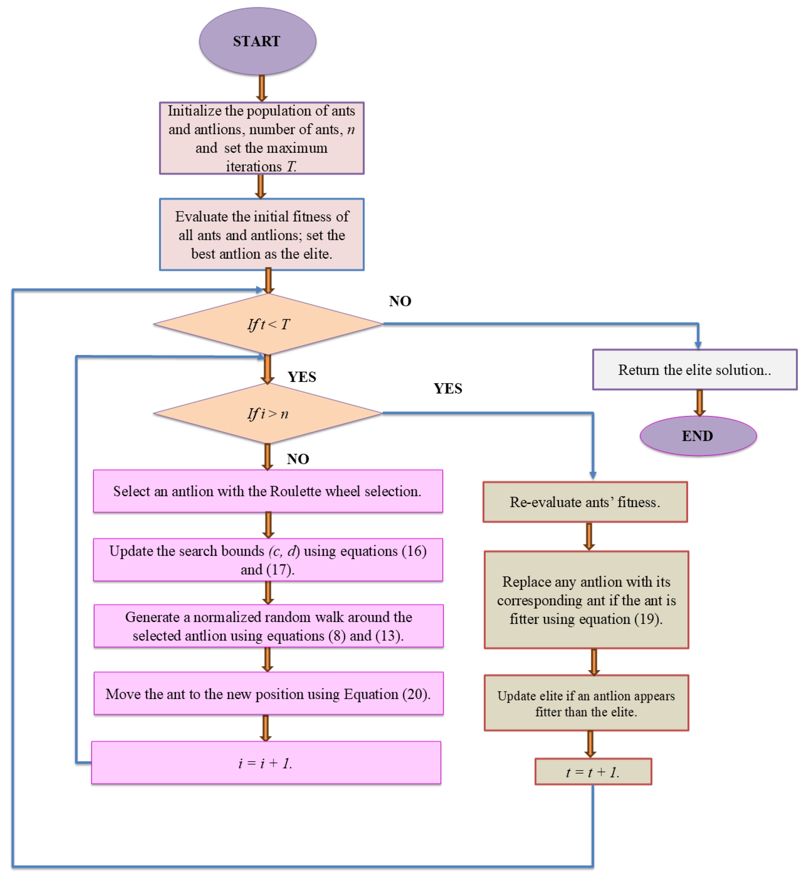
The optimisation flowchart for the ALO for a single objective optimisation is illustrated in Figure 4. After initializing ants and antlions, fitness is evaluated, and the best antlion is set as the elite. For each iteration t =T, the Roulette wheel is used to select a guiding antlion, and the search bounds c, d are updated. Generate a normalized random walk around the selected antlion and elite, map it to the bounds c and d and update the ant’s position to advance the loop index, i. Re-evaluate ants, let the fitter ant replace its paired antlion, and the elite if a better antlion is discovered. Repeat until t = T and return the elite solution.
Figure 4.
Flowchart of the single-objective Ant Lion Optimizer (ALO).
However, a problem can have multiple conflicting objective functions in energy systems. This will require a multi-objective optimisation approach to simultaneously generate viable solutions. The multi-objective antlion optimisation (MOALO), modelled after the multi-objective particle swarm optimisation (MOPSO), integrates a mechanism for archive management and leader selection. Solutions are selected from a pre-defined archive size to improve solution diversity. Using the niching technique, a specified radius is employed to study the area of each solution and count nearby solutions as a measure of distribution. This ensures well-spread solutions within the archive. MOALO adopts two strategies, like MOPSO, to further enhance the distribution of solutions.
Firstly, the antlion is selected based on the solution with the least crowded neighbourhood. Equation (21) determines the probability of selecting a particular solution from the archive [19].
(21)
= constant value greater than 1
= number of solutions in the neighbourhood for the ith solution.
The second strategy deletes solutions from the most crowded neighbourhood when the archive is full to make space for new solutions. Equation (22) is used to identify which solution is likely to be deleted from the archive.
(22)
Finally, equation (15) needs to be modified for multi-objective problems. Equation (17) must also be modified to select a non-dominated solution from the archive on the simultaneous selection of antlions and elites.
The flowchart for the resulting mathematical model for multi-objective ALO is shown in Figure 5. From Figure 5, the MOALO variant balances exploitation and exploration while preserving diversity using an external archive. At each iteration, the parent antlion and elites are pulled from the archive by the Roulette wheel selection. The ants take normalized walks around the selected antlion and the elite within adaptive bounds, advancing towards non-dominated regions. After each iteration, the newly found non-dominated solutions refresh and update the archive. When the archive is full, equation (21) is used to prune densely packed members to preserve spread along the Pareto front. The algorithm terminates at t = T and returns the final nondominated archive, Pareto-optimal set.
2.6. Mathematical Formulation
The Ant Lion Optimiser (ALO) and its multi-objective version (MOALO) are utilised here to optimise the thermodynamic performance of a single-stage dual-bed silica gel–water ADC. ALO and MOALO are modelled on the hunting techniques of antlions in sand pits. Equations (2), (4) and (6) represent the regression-based models for the Coefficient of Performance (COP), Cooling Capacity (), and Waste Heat Recovery Efficiency () [23]. ALO/MOALO employs a stochastic evolutionary approach that emulates ant–antlion interactions to explore and exploit the design space.
The single-objective formulation of ALO optimises each objective independently.
- COP maximisation:
(23)
Similarly, the optimisation of Cooling Capacity () is defined as:
- Cooling capacity maximisation:
(24)
- Waste heat recovery efficiency maximisation:
(25)
To preserve the diversity among solutions, MOALO extends the ALO framework by using Pareto dominance, elitism, and a crowding distance mechanism to converge toward a diverse and optimal set of non-dominated solutions.
The multi-objective formulation simultaneously combines the three objectives as equation (26):
Maximise (26)
subject to the variable bounds:
[oC]
[oC]
[oC]
[kgs⁻¹]
[kgs⁻¹]
[kgs⁻¹]
[kgs⁻¹]
[W/K]
[W/K]
[W/K]
3. Results
3.1. Single Objective Optimisation
The single-objective ALO algorithm implemented in this study was adapted from the original work by Mirjalili et al [32] which is available online. The algorithm was tailored to the characteristics of the three objective functions, the selected decision variables and implemented on the MATLAB R2021a platform using a 64-bit operating system, an x64-based processor, 8 GB RAM, and a 12th Gen Intel(R) Core (TM) i7-1255u CPU @ 1.70 GHz laptop.
Although the operating envelopes generated by ALO in this study are high, they are plausible given the sink and source temperatures and UA values. Depending on the design conditions, experimental single-stage silica-gel/water units generally report COP between 0.3 to 0.5 [33]. A review study on silica-gel water ADCs reported a COP of approximately 0.5 – 0.6 and beyond for optimized cases [34]. This validates the results from the SOO ALO of this study. The observed trends need not match the linear marginal coefficients since they reflect re-optimized Pareto set solutions.
The actions are to maximize each of the objectives discussed under setpoints, Loop flow controls, heat exchanger (HX) UA practices, and a prioritized sequence for constrained conditions.
3.1.1. Coefficient of Performance (COP) Maximization
The ALO algorithm was used to solve equation (23) to determine the conditions for maximum COP, using the decision variables and values presented in Table 2. Table 3 displays the optimum decision variables to maximise COP, and . Based on the ALO Maximize COP solution from Table 3; the following actions can be adapted to interpret the optimizer’s choices into chiller-operable settings.
To achieve the optimal COP of 0.67412, the following control strategies were identified based on the direction of decision variables:
Setpoints to Target (COP Mode)
Moving the three temperature levers in the recommended favourable directions can immediately increase the COP.
Water-Loop Flows Setpoints
Driving the four water flow control loops towards the recommendations stated below can increase COP and UA effectiveness with diminishing returns. Flow meters with a Proportional Integral Derivative (PID) controller to command the Variable Frequency Drive (VFD) speed can be used to achieve each ALO specified flow rate.
Thermal Conductance (UA) Operational Levers
From Table 3, the ALO optimum shows high UA values. While UA is primarily design-fixed [22] effective UA depends on the following steps:
- maximize , , or operate closer to high UA values [38].
- Open all HX circuits, balance flows and keep filters clean.
- Defoul evaporator and condenser surfaces on schedule.
- Maintain high tower airflow and adequate cooling water velocity.

Table 3.
ALO single-objective optima for COP, and ; metrics on the right are the values for the same solution.
Table 3.
ALO single-objective optima for COP, and ; metrics on the right are the values for the same solution.
| Optimization Objective | Decision Variable Values (from ALO) | Resulting COP[−] | Resulting[kW] | Resulting[−] |
| Maximize COP |
= 95°C, = 22°C, = 20°C, = 2.20 kgs⁻¹, = 2.2 kgs⁻¹, = 1.4 kgs⁻¹, = 2.2 kgs⁻¹, = 10000 W/K, = 10000 W/K, = 24000 W/K |
0.67412 (Max Value) | NR | NR |
| Maximize |
= 95°C, = 22°C, = 20°C, = 2.20 kgs⁻¹, = 2.135 kgs⁻¹, = 1.4 kgs⁻¹, = 2.2 kgs⁻¹, = 10000 W/K, = 10000 W/K, = 23999.66 W/K |
NR | 18.2235 (Max Value) | NR |
| Maximize |
= 65°C, = 22°C, = 20°C, = 2.198 kgs⁻¹, = 1.658 kgs⁻¹, = 1.396 kgs⁻¹, = 1.244 kgs⁻¹, = 10000 W/K, = 10000 W/K, = 23738.26 W/K |
NR | NR | 0.11829 (Max Value) |
Priority When Constrained (Most COP per Effort)
When it is impossible to achieve all targets (ambient and equipment limits), leverage the following steps for the biggest COP gain per step.
- : lower to make the sink colder and reduce the tower approach to wet bulb.
- UA: increase all UA through cleaning HX or balancing flow.
- and Push and further. Although this could reduce , it can increase COP when sink and UA are in good shape.
- : Fine-tune . Too low will starve the evaporator duty, and too high will reduce Logarithmic Mean Temperature Difference (LMTD), so it is better to stay near the ALO target of around 1.4 kgs⁻¹.
3.1.2. Cooling Capacity () Maximization
To identify the conditions for maximum , the ALO algorithm was used to solve Equation (24) with the decision variables and values from Table 2. Table 4 displays the optimum decision variables to maximise . To achieve a maximum of 18.2235 kW, the following variable adjustments depicted in Table 3 are required.
Setpoints to Target ( Mode)
Moving the three temperature levers in the recommended favourable directions can immediately increase the .
Water-Loop Flows Setpoints
Driving the flow control loops towards the recommendations stated below can increase COP and UA effectiveness with diminishing returns.
Thermal Conductance (UA) Operational Levers
From Table 3, the ALO optimum shows high UA values. While UA is primarily design-fixed [22], effective UA depends on the following steps:
- maximize , , or operate closer to high UA values [38].
Priority When Constrained (Most kW per Effort)
When it is impossible to achieve all targets (ambient and equipment limits), leverage the following steps for the biggest gain per step.
- UA: increase all UA through cleaning HX or balancing flow.
- and Increase and within limits to enhance the drive heat and increase [35].
- and : Raise and to increase evaporator throughput and lower condenser temperature, respectively. It is advisable to keep close to the ALO target of around 1.4 kgs⁻¹. This can directly increase [37].
3.1.3. Waste Heat Recovery Efficiency () Maximisation
Applying the ALO algorithm to Equation (25) with the decision variables and values from Table 2 yielded the results in Table 3. To achieve a maximum of 0.11829 requires the following set points.
Setpoints to target ( mode)
Moving the three temperature levers in the recommended favourable directions can immediately increase the .
- : reduce toward 65 °C with other favourable settings to increase . However, too low weakens desorption to reduce . This shows that to some extent, "higher is not always better" for and there exists an optimum.
- should be low enough to keep the sink cold and support desorption, but not weaken it (around 22 °C) [43].
- increase to around 20 °C. This will reduce the temperature lift to increase to its optimum [43].
Water-Loop flows setpoints
Combining the recommendations stated below with Proportional Integral Derivative (PID) and Variable Frequency Drive (VFD) speed flow meters can achieve each ALO specified flow rate to boost .
- : aim for moderate to high (2.198 - 2.20 kgs⁻¹) to sustain desorption at the lower without "over-supplying" heat [35].
- aim for a moderate flow rate (around 1.658 kgs⁻¹), just enough to maintain without increasing the drive heat and number of transfer units (NTU), diminishing returns [44].
- moderate to low (around 1.244 kgs⁻¹) to maintain consistent heat rejection and higher [44].
Thermal Conductance (UA) Operational Levers
From Table 3, the ALO optimum shows high UA values. While UA is primarily design-fixed [22], effective UA depends on the following steps:
- and : Keep and high around 10,000 kW/k. Better HX effectiveness directly relates to increased cooling for the same drive heat, thereby increasing [44].
- Cleaning the condenser, adequate tube/channel velocity and balanced circuits can increase the effectiveness of UA without an excessive increment of the operating values.
Priority When Constrained (Most ηₑ per Unit Drive Heat)
When it is impossible to achieve all targets (ambient and equipment limits), leverage the following steps for the biggest gain per step.
- Enable a lower . Reduce the temperature lift by reducing and increasing [43]Increasing (within process limits) increases evaporating saturation pressure/temperature to reduce lift. The resulting LMTD is enough to maintain or slightly increase evaporator duty without suppressing .
- Aim for between 65–75 °C at a minimum acceptable . Efficiency has been reported to peak at moderate temperature drives [35].
3.1.4. Conflicts in Single-Objective Optima (ALO)
From Table 4, the linear surrogate models indicate a monotone direction. Under box constraints, maximising a single objective drives all the positively signed coefficients to their upper bounds while dragging down all the negatively signed variables to their lower bounds. For instance, since in shows opposite signs in versus COP/Qcc, the SOO optima are mutually incompatible and different. Varying across its admissible bounds (65 - 95 °C) while holding other variables fixed, increased COP by +0.042 and Qcc by +9.32 kW, while decreasing by -0.009. This model-level antagonism necessitates an MOO approach to show a full Pareto front rather than isolating corner solutions.
Unlike MOALO, which constructs a Pareto front of all objectives [19], ALO conceals the continuous trade-off surface while exposing only the isolated extreme points of the decision variable bounds [28].
Table 4 reports the response model of the linear regression’s directional preferences of each objective at its single-objective optimum in maximisation form. An upward arrow, “↑” indicates that the objective increases when the variable moves towards its upper bound and a downward arrow “↓” implies there is an improvement when the objective moves towards its lower bound. The conflicts column shows consensus, “✓” when all three objectives have the same direction and “≠” indicates conflict when at least one objective goes the opposite direction (e.g., ↑, ↑ ↓,). For this model, reduces but increases COP and Qcc, which is a conflict and requires a multi-objective (Pareto) treatment.
Table 4.
Trend of Decision Variables under ALO-Based SOO.
| Decision Variable | Symbol | COP | Conflict | ||
| Hot-water inlet temperature | ↑ | ↑ | ↓ | ≠ | |
| Cooling-water inlet temperature | ↓ | ↓ | ↓ | ✓ | |
| Chilled-water inlet temperature | ↑ | ↑ | ↑ | ✓ | |
| Hot-water mass flow rate | ↑ | ↑ | ↑ | ✓ | |
| Bed cooling-water mass flow | ↑ | ↑ | ↑ | ✓ | |
| Chilled-water mass flow | ↑ | ↑ | ↑ | ✓ | |
| Condenser cooling-water mass flow | ↑ | ↑ | ↑ | ✓ | |
| Bed overall conductance | ↑ | ↑ | ↑ | ✓ | |
| Evaporator overall conductance | ↑ | ↑ | ↑ | ✓ | |
| Condenser overall conductance | ↑ | ↑ | ↑ | ✓ |
Legend: ↑ increases at optimality; ↓ decreases; ≠ conflict.
Table 4 confirms that the best way to maximise one objective (e.g., ) differs from the optimal direction to maximise another (e.g., COP or ) for certain decision variables like and . This implies that no single set of operating parameters can simultaneously maximise all the three performance metrics. This necessitates determining the Pareto optimal solutions through multi-objective optimisation (MOO), such as the Multi-Objective Ant Lion Optimiser (MOALO). Using MOALO goes beyond merely finding isolated optimal points for individual objectives; it identifies a set of non-dominated solutions that represent the best trade-offs among these competing performance metrics [19].
3.2. Multi-Objective Optimisation
The multi-objective antlion optimisation algorithm implemented in this study was adapted from the original work by Mirjalili et al [46], which is available online. The algorithm was tailored to the characteristics of the three objective functions, the selected decision variables and implemented on the MATLAB platform using a 64-bit operating system, an x64-based processor, 8GB RAM, and a 12th Gen Intel(R) Core (TM) i7-1255u CPU@ 1.70 GHz laptop. The set values of the hyperparameters, as proposed by Mirjalili et al. [100] in the original MOALO algorithm, are provided in Table 5.
3.2.1. Pairwise Pareto Front Trade-offs (2-D Projections)
Across the investigated bounds, the front is effectively one-dimensional (1-D) and collapses to form a ridge. Rather than a broad, multi-dimensional surface, the two-dimensional (2-D) plots show the data points as a narrow continuous linear curve. For panel (a), COP increases monotonically with , yielding an almost continuous linear curve, whereas is non-correlated with both capacity (panel b) and COP (panel c). Panels (b) and (c) show that reduces as either COP or increases, validating the plot in panel (a) and indicating a consistent trade-off between COP/cooling capacity and . Altogether, the three projections demonstrate that aiming for a higher COP and will be at the cost of and vice versa. A practical design compromise is seen near the intersections of panels (a) to (c), as a balanced region is identified around COP ≈ 0.695, ≈ 24 kW, and ≈ 0.122–0.123. Figure 6
3.2.2. Validation of Objective Models and Pareto-Front Quality
Within the explored bounds, the COP, , and fronts compress towards an effective 1-D manifold because the objectives co-vary with the same hot-side driving temperature potential and heat-transfer conductance (UA). The performance of classic silica-gel/water systems ADCs is significantly affected by heat and mass flow rates [47], and both the COP and cooling capacity are very sensitive to operating water temperatures [48]. This coupling inherently results in a ridge-shaped front geometry. Nevertheless, a ridge-shaped front is expected because the objectives are correlated and partially redundant due to the degeneration of the Pareto fronts for such regimes [49,50]. This is why the results are presented in 2-D rather than 3-D to ensure the plots are clear and free from occlusion for quantitative comparison [47,49]. The observed trends in the 2-D projections are physically plausible and internally consistent with the working of silica-gel/water systems ADCs. Cooling capacity increases as hot water (desorption) temperature rises until an optimum efficiency, after which COP may decline [35,51,52,53]. As noted earlier, observed trends reflect re-optimized Pareto sets and do not necessarily correspond to linear marginal coefficients; therefore, moving from one Pareto-optimal solution to another indicates a trade-off [54,55].
All reported Pareto data points meet the imposed bound limits (temperatures, mass-flow rates, and UA products) and basic thermodynamics constraints, as the approach temperatures are realistic and there are monotonic responses to driving temperature and heat transfer area. There are no remaining infeasible or dominated points after re-evaluation [35].
Table 6 summarizes selected literature benchmarks for ADC performance and compares them with the MOALO Pareto set across COP, , operating temperatures and system scale. The MOALO front yields COP from 0.69–0.71, around 18–27.3 kW, and operating temperature from 65–95 °C for , around 22 °C and 20 °C aligning with reported values [56,57,58,59]. Even though was derived from a prior formulation, it is seldom reported as a performance metric in ADC optimization. It is therefore reported explicitly for this MOALO Pareto solutions within the explored bounds as 0.118–0.1275 (11.8–12.75%) to provide a direct measure of utilization of waste heat for design and comparison. The reported ranges of add useful context for future waste-heat integration studies while remaining consistent with the underlying thermodynamics principles. Overall, the reported literature aligns with the results from this study and supports the quality of the generated MOALO Pareto set and the reliability of the objectives.
3.3. Sensitivity Analysis
To assess the robustness of the MOALO results, a One-at-a-Time (OAT) approach sensitivity analysis (SA) was conducted to examine the impact of each decision variable on COP, , and . One variable was swept across the lower, midpoint, and upper bounds, while all other variables were held at their baseline values. For each OAT setting, the optimizer was re-run for twenty independent runs using the same hyperparameters to obtain a stable Pareto set [62,63]. After each run, the resulting non-dominated cloud of Pareto-optimal points for the objectives was summarized, with cubic polynomial fits. The trends are reported as three projections: against COP, against COP and ηₑ against .
3.3.1. Effects of Varying Hot Water Inlet Temperature
Figure 7 illustrates the effects of on the Pareto set. Three levels are shown as 65 °C (low, blue circles), 80 °C (intermediate, red squares), and 95 °C (highest, green triangles). The markers represent the non-dominated solutions, and smooth curves are cubic fits drawn to guide the eye. In panel (a), COP increases with . across all Thwin. This shows a positive correlation between COP and . within the explored bounds, consistent with prototype and bench tests of silica-gel/water units [60,64].
For panels (b) and (c), shifts upwards as rises. Higher usually, improves the desorption process and increases the useful cooling per unit bed up to an intermediate optimum beyond which gains decline [60,65]. The –COP relation is a concave curve with a maximum occurring at a COP between 0.78 and 0.82, in line with the reported optimum driving temperature behaviour for silica-gel/water systems ADCs [60,66].
Panel (c) suggests diminishing returns in waste heat utilization as initially increases with higher ., then saturates more prominently at 80–95 °C. Literature confirms that the performance of declines beyond an optimum driving force at larger throughput [60,67]. Practically, datasheet operating windows support the use of 65–95 °C for ADCs and highlights performance flattening at the upper end [68]
Within the MOALO envelope, if maximizing waste heat utilization is the priority, then the ADC should be operated at a higher (80–95 °C) around the intermediate COP region where peaks, as specified by the datasheet operating windows [68]. If cooling capacity is the main requirement, a trade-off is observed in panel (c) for . and. Thus, 65 °C can deliver a higher at the expense of . Depending on the available source temperature, this study offers a balanced compromise around a COP of 0.80, with . between 28–34 kW and , 0.150–0.170 at 95°C.
3.3.2. Effects of varying cooling water inlet temperature on the Pareto set
Figure 8 illustrates the effects of on the Pareto set. Three OAT levels are shown as 22 °C (low, blue circles), 29 °C (intermediate, red circles), and 36 °C (highest, green circles). The markers represent the non-dominated solutions from re-optimised runs. In panel (a), . increases alongside COP for every within the explored bounds. clearly separates the Pareto clouds. The MOALO optimizer adjust the other degress of freedom to compensate so the highest COP and . are observed at 36 °C, followed by 29 °C and 22 °C. In most fixed envelope silica-gel/water ADCs experimental settings, increasing usually degrades . and COP, so the ordering of here reflects re-optimization rather than a universal law [56,66,69,70].
In panel (b), a negative correlation is observed within each level. decreases as COP rises. The MOALO optimizer compensation shifts the entire -COP curve upwards across all levels (36 °C > 29 °C > 22 °C). Under fixed conditions, increasing is generally detrimental to the performance of the ADC [56,66,69]. The observed trends are specific to the explored bounds and OAT protocols, where the optimizer reallocates other variables as varies. From panel (c), higher corresponds to higher across all levels, while decreases with .
Again, in these OAT runs, the MOALO optimizer adjusts responses to changes in Thus, fixed-setting studies will report the opposite ordering when other variables are held constant [56,66,69,70]. These trends highlight the practical limitations and sensitivity to sink conditions as indicated in the datasheet windows [57,58,68].
In this MOALO envelope, a balanced design compromise is observed around COP 0.79–0.82, with .between 31 and 38 kW and ηe approximately 0.140–0.155.
3.3.3. Effects of Varying Chilling Water Inlet Temperature on the Pareto Set
Figure 9 illustrates the effects of on the Pareto set. Three OAT levels are shown as 10 °C (low, blue circles), 15 °C (intermediate, red circles), and 20 °C (highest, green circles). The markers represent the non-dominated solutions from re-optimised runs, and no curve fits are shown. In panel (a), . and COP increase together across all levels of . The fronts are ordered by . The highest 20 °C (blue), shows the highest COP–, followed by 15 °C (red) and 10 °C (green). This ordering aligns with the behaviour of silica-gel/water ADC under fixed settings, where both COP and . improve due to a reduction in temperature lift from warmer chilled water law [56,60,69].
For panel (b), slightly decreases as COP increases within each level. Across levels, lower temperature lifts improve heat utilization at the hot side, so higher swings the whole -COP band upwards (20 °C > 15 °C > 10 °C) [56,66,69]. In panel (c), warmer chilled water produces higher values, while decreases with COP for each level of . Similar shifts and sensitivity of returning/leaving chilled water temperatures are documented in manufacturer datasheets [57,58,68].
For this MOALO study, the Pareto front is favourable for processes that can accept chilled water at higher temperatures to produce higher COP, . and. However, expect a reduction in the COP and values if the requirement is a strict = 10 °C set point. Within the explored bounds of this study, a practical compromise lies around a COP of 0.80, with 29–35 kW and 0.145–0.158.
3.3.4. Effects of Varying Hot Water Inlet Mass Flow Rate on the Pareto Set
Figure 10 (a-c) reveal how changing the hot water mass flow rate ( ) at three different levels, 0.8 kgs⁻¹ (black circles), 1.5 kgs⁻¹ (orange squares), and 2.2 kgs⁻¹ (green triangles), affects system performance. Panel (a) shows the COP against . across the tested flow rate range. The upper part of the plot is predominantly occupied by the highest-flow set ( = 2.2 kgs⁻¹, green triangles), suggesting a strong, positive linear correlation between COP and, while the lowest-flow set ( = 0.8 kgs−1, black circles) lies lower. However, the three MOALO clouds are tightly clustered.
This indicates that the hot water mass flow rate has weak leverage on the core COP-. performance within the tested envelope. This agrees with Kalawa et al [71], who found that increasing the mass flow rate marginally improves COP/, albeit improving operational stability.
Theoretically, higher improves heat transfer and desorption rate in silica gel–water ADC systems [24]. But, this MOALO optimizers likely compensate via other degrees of freedom, resulting in the observed weak sensitivity. Panel (b) shows against COP, and panel (c) against . The plots show clear stratification based on the flow rate. decreases as COP or . increases within each flow rate level. There is a significant monotonic decline in ηₑ as increases across each level ( : 0.8 > 1.5 > 2.2 kg s−1). Theoretically, a higher quickens the desorption process, resulting in a faster cooling cycle and potentially better cooling performance [24]. Nevertheless, they can also intensify irreversibilities and increase entropy generation, leading to losses in useful energy that decrease the quality of ηₑ [72]. This results in a trade-off: modest COP or gains at high at the cost of lower . These trends mirror reoptimized solutions and are specific to this envelope. Operate at a lower when waste heat is costly or limited to maintain a high at a smaller . A higher is preferable if is the limiting factor but expect a lower . A practical compromise for a reasonable . and moderate is to use the mid-flow level (1.5 kgs⁻¹) near the mid-COP region.
3.3.5. Effects of Varying Bed Cooling Water Mass Flow Rate on the Pareto Set
Panels (a-c) show the effects of bed cooling water mass flow on the Pareto set at three levels: 0.8 kgs⁻¹ (black circles), 1.5 kgs⁻¹ (orange squares), and 2.2 kgs⁻¹ (green triangles). Markers represent non-dominated solutions.
Panel (a) against COP shows an improvement in the ADC’s primary cooling performance as increase. The lowest performance occurs at the lower region ( = 0.8 kg s⁻¹), while the highest-flow band ( = 2.2 kg s⁻¹) occupies the upper region, with COP up to 0.73 and around 28.5 kW. This is thermodynamically reasonable, as a higher bed cooling water mass flow facilitates effective removal of adsorption heat. This reduces the bed pressure during adsorption and maintains vapour uptake to increase throughput. Consequently, COP increases with but with diminishing returns at higher flow rates [24].
Conversely, panels (b) against COP and (c) against shows a decrease in waste heat efficiency (ηₑ) at higher both within and across all levels. Maximum occurs at the lowest flow rate (0.8 kgs⁻¹), while the highest flow rate (2.2 kgs⁻¹) results in the lowest ηₑ. At higher mass flow rates, the cooling water stream effectively dissipates more heat, but this increases irreversibilities too. Therefore, the quality of waste-heat utilisation falls even if improves [24,72]. Figure 11
3.3.6. Effects of Varying Chilled Water Inlet Mass Flow Rate on the Pareto Set
Panels (a-c) show the effects of chilled water mass flow on the Pareto set at three levels: 0.2 kgs⁻¹ (black circles), 0.8 kgs⁻¹ (orange squares), and 1.4 kgs⁻¹ (green triangles). Markers are non-dominated solutions.
Panel (a) shows against COP. The lowest (0.2 kgs⁻¹) corresponds to the highest COP values (0.78 to 0.83) and the highest (28 to 32 kW). The intermediate (0.8 kgs⁻¹) shows mid-point values for both COP and . And the least COP and values are observed at high (1.4 kgs⁻¹). Although increasing generally improves heat transfer, the plots show the existence of a low to mid flow optimum on the evaporator side and going beyond that can have detrimental effects on the off-design operation of the components. Sah et al reported a near-flat trend of performance metrics at higher chilled water flow rates and improvement at low to moderate flow rates, indicating diminishing returns and an implied optimum [40]. Figure 12
Panels (b) against COP and (c) against . An inverse relationship is observed between and COP or within each level. decreases as COP or increases. Raising the chilled-water flow from 0.8 to 1.4 kgs⁻¹ produced a lower COP and Qcc. This is due to operating beyond the evaporator-side optimum, where the bedside heat/mass-transfer limits the performance. Beyond the optimal operating conditions, the effective LMTD/residence time reduces, declining evaporative duty per cycle as increasing flow rate causes a marginal rise in thermal conductance. This behaviour is consistent with the finite time module and bed transport limits characteristics of adsorption modules [44,73] and saturation of gains at higher mass flow rates [20].
Within the explored bounds, choosing low to mid when COP and are the priorities can preserve . However, operating at very pushes the ADC beyond the evaporator-side optimum and penalizes both COP and . Practically, a balanced compromise will be to run at 0.8 kg s⁻¹ close to COP of 0.76–0.80.
3.3.7. Effects of Varying Condenser Cooling Water Mass Flow Rate on the Pareto Set
Panels (a-c) show the effects of condenser-cooling mass flow on the Pareto set at three levels: 0.8 kgs⁻¹ (black circles), 1.5 kgs⁻¹ (orange squares), and 2.2 kgs⁻¹ (green triangles). Markers are non-dominated solutions, and other variables are held at baseline and reoptimized.
Panel (a) against COP. A clear positive coupling is observed for and COP. Increasing shifts the entire cloud upwards and increases with COP. An increase in improves heat dissipation from the condenser and reduces the average condensing temperature (smaller lift). This raises the at a given COP. A modest separation is identified with diminishing returns at the highest This is consistent with off-design limits and sink-side improvements characteristics for silica-gel/water ADCs [56,69].
Panel (b) shows against COP, and (c) against . An inverse relationship is seen for and across all levels, whiledecreases with COP or as increases within each level. Figure 13
Similarly to the case, rejecting more heat in the sink increases entropy generation and thus, the quality of waste heat used falls while COP or improves [40,56,72].
If is the ADC’s priority, then a higher is beneficial, and if is the main requirement, then a lower is most preferable. Within the explored envelope, operating at mid flow (1.5 kg s−1) near the mid COP is a good compromise, which gives higher at a moderate penalty.
3.3.8. Effects of Varying Bed Overall Conductance on the Pareto Set
Panels (a-c) show the effects of overall bed thermal conductance on the Pareto set at three levels: 2,000 W/K (low, purple circles), 6,000 W/K (mid, teal diamonds), 10,000 W/K (high, red squares). Markers are non-dominated solutions, and other variables are held at baseline and reoptimized for each level.
Panel (a) shows against COP. The three bands are almost parallel and increasing shifts the cloud up and to the right to yield a higher COP at a given and a higher at a given COP. Physically, a higher UA increases the effectiveness of removing heat of adsorption. Figure 14
Panels: (a) versus COP; (b) versus COP; (c) versus This improves regeneration and reduces bed temperature during adsorption and temperature swings during desorption to increase the cycles' and COP [24,52,56,74].
Panel (b) shows against COP, and panel (c) shows against . Within each lever, reduces as COP or rises but increases monotonically with across all levels. Larger UA reduces the temperature approach differences, thereby reducing irreversibilities and improving the quality of heat utilization [72,74,75].
However, the spacing between each band narrows at high , suggesting internal limitations and diminishing of gains once the external HX resistance reduces [24,76].
Within the explored bounds, increasing raises COP, and until internal limits set in. Practically, a balanced compromise will be at the mid to high range of 6000 –10000 W/K near the mid-COP region, which yields high with a good . Pushing above 10000 W/K only improves slightly relative to the size and/or cost constraints.
3.3.9. Effects of Varying Condenser Overall Conductance on the Pareto Set
Panels (a-c) illustrate the influence of condenser overall conductance on the Pareto set at three levels: 10,000 W/K (low, purple circles), 17,000 W/K (mid, teal diamonds), 24,000 W/K (high, red squares). Markers represent non-dominated solutions, with other variables held at baseline and reoptimized for each level. Figure 15
Panel (a) shows against COP. The plots reveal three nearly parallel bands that shift upward and to the right as increases. COP slightly improves for a given , while significantly increases for a given COP. Higher condenser UA reduces heat rejection, lowers the mean condensing temperature, and raises both and COP [24,52,74]. The narrow spacing between bands at high indicates diminishing returns.
Panel (b) depicts versus COP, and panel (c) shows against . In each band, decreases as COP or rises. An inverse relationship exists between a, because increasing results in more heat being dumped into the sink, raising entropy generation. Therefore, although improves, the quality of waste heat utilisation () declines [72,74].
When cooling capacity is paramount, a higher is the optimal choice. Conversely, if waste heat utilisation is the priority, low to moderate should be preferred to preserve . For this envelope, if the design requires high with a moderate penalty on , around 17000 W/K near the mid COP region would be a good compromise.
3.3.10. Effects of Varying Evaporator Overall Conductance on the Pareto Set
Panels (a-c) illustrate the influence of evaporator overall conductance on the Pareto set at three levels: 2,000 W/K (low, purple circles), 6,000 W/K (mid, teal diamonds), 10,000 W/K (high, red squares). Markers are non-dominated solutions, with other variables held at baseline and re-optimised for each level.
Panel (a) shows three nearly parallel bands that shift upward for against COP as decreases from 10,000 W/K to 6,000 W/K to 2,000 W/K. That is, for a given , there is a moderately higher COP, and for a given COP, there is a noticeably higher at lower . This implies that within this envelope, the evaporator is not the active bottleneck after re-optimisation, but MOALO compensate by reallocating the high-side temperatures and flow rates (other degrees of freedom) for a slightly lower COP and at higher . A higher usually raises the evaporation temperature (reduces lift) to increase [24,52,74].
Panel (b) is against COP. reduces as COP increases within each band in the order of 2,000 W/K, 6,000 W/K and 10,000 W/K across the band. High increases throughput and total heat dissipated to the sink, but raises irreversibilities, which lowers the quality of waste heat utilization [72,74].
Panel (c) displays against , following the same pattern as panel (b). decreases as increases within the bands across all levels. This reveals the inherent trade-offs between and . Raising to 10,000 W/K results in diminishing returns on the re-optimised Pareto front due to compensation. Thus, a good compromise for this OAT envelope is lower to mid (2000–6000 W/K) near the mid COP region for a higher at a comparatively higher . Figure 16
4. Conclusions
This study developed a computational framework to maximise the performance of a silica gel–water single-stage dual-bed adsorption chiller using Antlion Optimiser (ALO) and Multi-Objective Antlion Optimiser (MOALO). Regression models that have been statistically validated were used to formulate objective functions for three key performance indicators: Coefficient of Performance (COP), cooling capacity (), and waste heat recovery efficiency (). is introduced and treated as an equivalent objective (not a derived metric), just like COP and , and it is consistently taken through modelling, optimisation, visualisation and validation along with COP and . Furthermore, a structured validation and sensitivity analysis were carried out to ensure the optimisation framework's physical consistency and robustness.
The following is a summary of the study's findings and outcomes:
- MOALO identified the non-dominated set of decision variables influencing the performance of a single-stage dual-bed ADC. These included inlet temperatures, heat exchanger conductance, and mass flow rates.
- Three objective functions: COP, , and were formulated from statistically validated regressions and used to assess the performance of a single-stage dual-bed ADC. Treating as a primary objective explicitly emphasises waste heat utilisation in addition to conventional performance metrics.
- The optimal or non-dominated solutions produced by ALO and MOALO provide actionable trade-offs to enhance performance with COP ranging from 0.675–0.717, from roughly 18.3–27.5 kW, and reaching an approximated maximum range of 0.131, clustering around intermediate COP and values. The ALO and MOALO outcomes are consistent (and superior in some cases) to comparable literature benchmarks within the same operating window.
- References on experiments, commercial product datasheets, heat exchanger conductance and optimisation trade-offs were used to validate the objective functions and operating bounds.
- Although is seldom explicitly reported in ADC studies and validation benchmark tests, the achieved window demonstrates effective waste heat utilisation (recovery), contributing source-aware knowledge to existing literature.
- A one-at-a-time (OAT) sensitivity analysis was run, varying the focal variable at three levels (low, mid and high) while re-optimising all non-focal variables. Across objectives, , , and heat exchanger conductance ( and ), emerged as the most influential levers.
- Instead of 3-D projections of all three objectives, pairwise 2-D projections were used for visualisations to make interpretations of trade-offs easy and avoid occlusions of 3-D static projections. Within the explored bounds, the Pareto set is compressed to an effective 1-D ridge due to the inherent trade-offs between COP and and . falls as COP and/or rises.
- The results shown by each OAT panel are non-dominated solutions after re-optimising all non-focal decision variables. Therefore, the order by which results are presented at different lever levels must not be read as a fixed-point sensitivity where other variables are kept constant. The MOALO results reflect compensated design responses rather than simple single-parameter gradients and should be interpreted as such.
- If is the priority, it is recommended to operate at a higher , allow a slightly warmer if acceptable to the process to reduce the temperature lift, use adequately higher UA and avoid excessive heat dissipation that can penalise .
- On the other hand, if the priority is effective waste heat utilisation, a balanced compromise will be to operate near the intermediate-COP region, where peaks, while moderating sink side flow rates and UA. should be tuned to get a balanced and utilisation quality.
- Outside the explored envelope, linear regressions can exhibit non-physical intercepts, which require reciprocal transformation for SA convenience and interpretations. To ensure realistic performance predictions across the entire operating range, future research should focus on developing more physically constrained models, carrying out experimental validation at representative Pareto points, uncertainty quantification, and exploring alternative adsorbents and multi-bed recovery schemes.
- In conclusion, this study verifies the effectiveness of MOALO for improving ADC performance. Treating as a co-equal objective alongside COP and equips designers and decision makers with source-aware guidance to balance or prioritise cooling performance and waste heat utilisation within the established operating envelope. Thus, the regression-assisted MOALO framework may serve as a useful and practical digital technology for configuring low-grade heat ADCs and could be extended to other sustainable cooling processes.
Author Contributions
Conceptualization, P.K.-B. and L.T.; methodology, P.K.-B. and L.T.; formal analysis, P.K.-B.; investigation, P.K.-B.; resources, L.T.; writing—original draft preparation, P.K.-B.; writing—review and editing, L.T. and J.T.-C.; supervision, L.T. and J.T.-C.; project administration, L.T. All authors have read and agreed to the published version of the manuscript.
Funding
This research received no external funding.
Institutional Review Board Statement
Not applicable
Informed Consent Statement
Not applicable.
Data Availability Statement
The data presented in this study are available on request from the corresponding author due to ongoing doctoral research and institutional restrictions.
Conflicts of Interest
The authors declare no conflicts of interest.
Abbreviations
The following abbreviations are used in this manuscript:
ADCs Adsorption Chillers
MVC Mechanical Vapour Compression
COP Coefficient of Performance
GWO Grey Wolf Optimizer
MOGWO Multi-Objective Grey Wolf Optimizer
ALO Antlion Optimiser
MOALO Multi objective antlion optimiser
HFC Hydrofluorocarbon
HCFC Hydrochlorofluorocarbon
RAC Refrigeration and Air Conditioning
GHG Greenhouse Gas
SEER Seasonal Energy Efficiency Ratio
KPI Key Performance Indicators
PSO Particle Swarm Optimization
half cycle time
cp Specific heat capacity (kJ·kg⁻¹·K⁻¹)
k Thermal conductivity (W·m⁻¹·K⁻¹)
L Latent heat of vaporization (kJ·kg⁻¹)
ṁ Mass flow rate (kg·s⁻¹)
Cooling capacity at the evaporator (kW)
t Time (s)
T Temperature (°C; use K for ΔT)
UA Overall heat conductance (kW·K⁻¹)
Hot-water inlet temperature to adsorber/desorber (°C)
Cooling-water inlet temperature to condenser/adsorber (°C)
Chilled-water inlet temperature to evaporator (°C)
Hot-water mass flow rate (kg·s⁻¹)
Cooling-water mass flow rate through beds (kg·s⁻¹)
Chilled-water mass flow rate (kg·s⁻¹)
Cooling-water mass flow rate through condenser (kg·s⁻¹)
Bed heat exchanger conductance (kW·K⁻¹)
Evaporator conductance (kW·K⁻¹)
Condenser conductance (kW·K⁻¹)
References
- Calvin, K.; Dasgupta, D.; Krinner, G.; Mukherji, A.; Thorne, P.W.; Trisos, C.; Romero, J.; Aldunce, P.; Barrett, K.; Blanco, G.; et al. IPCC, 2023: Climate Change 2023: Synthesis Report. Contribution of Working Groups I, II and III to the Sixth Assessment Report of the Intergovernmental Panel on Climate Change [Core Writing Team, H. Lee and J. Romero (Eds.)]. IPCC, Geneva, Switzerland; First.: Geneva, Switzerland.; Intergovernmental Panel on Climate Change (IPCC), 2023. [Google Scholar]
- World Health Organization (WHO) Climate Change: Heat and Health (Fact Sheet) WHO. Available online: https://www.who.int/news-room/fact-sheets/detail/climate-change-heat-and-health (accessed on 17 November 2024).
- International Energy Agency (IEA) Staying Cool without Overheating the Energy System. Available online: https://www.iea.org/commentaries/staying-cool-without-overheating-the-energy-system (accessed on 24 August 2025).
- Randazzo, T.; De Cian, E.; Mistry, M.N. Air Conditioning and Electricity Expenditure: The Role of Climate in Temperate Countries. Economic Modelling 2020, 90, 273–287. [Google Scholar] [CrossRef]
- International Energy Agency World Energy Outlook 2024: Cooling Drives Electricity Demand. accessed on. (accessed on 24 August 2025).
- United Nations World Urbanization Prospects. Available online: https://www.un.org/development/desa/en/news/population/2018-revision-of-world-urbanization-prospects.html? (accessed on 24 August 2025).
- International Energy Agency Global Air Conditioner Stock. Available online: https://www.iea.org (accessed on 24 August 2025).
- Moran, M.J.; Shapiro, H.N.; Boettner, D.D.; Bailey, M.B. Fundamentals of Engineering Thermodynamics, 8th ed.; Wiley: Hoboken, N.J., 2014; ISBN 1-118-82044-4. [Google Scholar]
- Yunus Cengel, M.B.; Eighth, M. A.; Kanoglu, M. Thermodynamics: An Engineering Approach, 8th edition; McGraw-Hill Education, 7 January 2014; p. 1024. [Google Scholar]
- Graff Zivin, J.; Neidell, M. Temperature and the Allocation of Time: Implications for Climate Change. Journal of Labor Economics 2014, 32, 1–26. [Google Scholar] [CrossRef]
- Dupont, J.-L. The Role of Refrigeration in the Global Economy (2019), 38th Note on Refrigeration Technologies. Available online: https://iifiir.org/en/fridoc/the-role-of-refrigeration-in-the-global-economy-2019-142028.
- World Population Review Air Conditioning Usage by Country 2025. Available online: https://worldpopulationreview.com/country-rankings/air-conditioning-usage-by-country (accessed on 25 August 2025).
- International Energy Agency. The Future of Cooling: Opportunities for Energy-Efficient Air Conditioning. Available online: https://iifiir.org/en/fridoc/the-future-of-cooling-opportunities-for-energy-efficient-air-conditioning-4787 (accessed on 19 August 2025).
- Goetzler, William; Zogg, Robert; Young, Jim; Johnson, Caitlin. Alternatives to Vapor-Compression HVAC Technology. ASHRAE Journal 2014, 56, 12–23. [Google Scholar]
- Goyal, P.; Baredar, P.; Mittal, A.; Siddiqui, Ameenur.R. Adsorption Refrigeration Technology – an Overview of Theory and Its Solar Energy Applications. Renewable and Sustainable Energy Reviews 2016, 53, 1389–1410. [Google Scholar] [CrossRef]
- Mugnier, D.; Goetz, V. Energy Storage Comparison of Sorption Systems for Cooling and Refrigeration. Solar Energy 2001, 71, 47–55. [Google Scholar] [CrossRef]
- Alahmer, A.; Ajib, S.; Wang, X. Comprehensive Strategies for Performance Improvement of Adsorption Air Conditioning Systems: A Review. Renewable and Sustainable Energy Reviews 2019, 99, 138–158. [Google Scholar] [CrossRef]
- Cui, Y.; Geng, Z.; Zhu, Q.; Han, Y. Review: Multi-Objective Optimization Methods and Application in Energy Saving. Energy 2017, 125, 681–704. [Google Scholar] [CrossRef]
- Mirjalili, S.; Jangir, P.; Saremi, S. Multi-Objective Ant Lion Optimizer: A Multi-Objective Optimization Algorithm for Solving Engineering Problems. Applied Intelligence 2017, 46, 79–95. [Google Scholar] [CrossRef]
- Kwakye-Boateng, P.; Tartibu, L.; Jen, T. Performance Optimization of a Silica Gel–Water Adsorption Chiller Using Grey Wolf-Based Multi-Objective Algorithms and Regression Analysis 2025.
- Critoph, R.E. Evaluation of Alternative Refrigerant—Adsorbent Pairs for Refrigeration Cycles. Applied Thermal Engineering 1996, 16, 891–900. [Google Scholar] [CrossRef]
- Miyazaki, T.; Akisawa, A. The Influence of Heat Exchanger Parameters on the Optimum Cycle Time of Adsorption Chillers. Applied Thermal Engineering 2009, 29, 2708–2717. [Google Scholar] [CrossRef]
- Papoutsis, E.G.; Koronaki, I.P.; Papaefthimiou, V.D. Parametric Study of a Single-Stage Two-Bed Adsorption Chiller. J. Energy Eng. 2017, 143, 04016068. [Google Scholar] [CrossRef]
- El-Sharkawy, I.I.; AbdelMeguid, H.; Saha, B.B. Towards an Optimal Performance of Adsorption Chillers: Reallocation of Adsorption/Desorption Cycle Times. International Journal of Heat and Mass Transfer 2013, 63, 171–182. [Google Scholar] [CrossRef]
- Griffiths, D. Pit Construction by Ant-Lion Larvae: A Cost-Benefit Analysis. The Journal of Animal Ecology 1986, 55, 39–39. [Google Scholar] [CrossRef]
- Scharf, I.; Subach, A.; Ovadia, O. Foraging Behaviour and Habitat Selection in Pit-Building Antlion Larvae in Constant Light or Dark Conditions. Animal Behaviour 2008, 76, 2049–2057. [Google Scholar] [CrossRef]
- Mani, M.; Bozorg-Haddad, O.; Chu, X. Ant Lion Optimizer (ALO) Algorithm; 2018; pp. 105–116. [Google Scholar]
- Mirjalili, S. The Ant Lion Optimizer. Advances in Engineering Software 2015, 83, 80–98. [Google Scholar] [CrossRef]
- Scharf, I.; Ovadia, O. Factors Influencing Site Abandonment and Site Selection in a Sit-and-Wait Predator: A Review of Pit-Building Antlion Larvae. Journal of Insect Behavior 2006, 19, 197–218. [Google Scholar] [CrossRef]
- Grzimek, B.; Schlager, N.; Olendorf, D.; McDade, M. Grzimek’s Animal Life Encyclopedia., Second. ed; Gale Farmington Hills: Michigan, 2004; Vol. 12. [Google Scholar]
- Goodenough, J.; McGuire, B.; Jakob, E. Perspectives on Animal Behavior, 3rd ed.; Wiley, 2009; p. 544. [Google Scholar]
- Seyedali Mirjalili Ant Lion Optimizer (ALO) 2025.
- Kiplagat, J.K.; Wang, R.Z.; Oliveira, R.G.; Li, T.X.; Liang, M. Experimental Study on the Effects of the Operation Conditions on the Performance of a Chemisorption Air Conditioner Powered by Low Grade Heat. Applied Energy 2013, 103, 571–580. [Google Scholar] [CrossRef]
- Bhargav, H.; Awasti, S.; Saniyawala, U.; Raulji, A.; Shah, S. A Review on Solar Adsorption Chiller Using Silica Gel Water Mixtures. SSRN Electronic Journal 2019. [Google Scholar] [CrossRef]
- Rezk, A.R.M.; Al-Dadah, R.K. Physical and Operating Conditions Effects on Silica Gel/Water Adsorption Chiller Performance. Applied Energy 2012, 89, 142–149. [Google Scholar] [CrossRef]
- Hua, Z.; Cai, S.; Xu, H.; Li, S.; Tu, Z. Investigating the Performance of Adsorption Chiller Operating under Fluctuating Heat-Source Conditions. Case Studies in Thermal Engineering 2025, 68, 105903–105903. [Google Scholar] [CrossRef]
- Makahleh, F.M.; Badran, A.A.; Attar, H.; Amer, A.; Al-Maaitah, A.A. Modeling and Simulation of a Two-Stage Air-Cooled Adsorption Chiller with Heat Recovery Part II: Parametric Study. Applied Sciences 2022, 12, 5156–5156. [Google Scholar] [CrossRef]
- Cacciola, G.; Restuccia, G.; van Benthem, G.H.W. Influence of the Adsorber Heat Exchanger Design on the Performance of the Heat Pump System. Applied Thermal Engineering 1999, 19, 255–269. [Google Scholar] [CrossRef]
- Liang, J.; Zhao, W.; Wang, Y.; Ji, X.; Li, M. Effect of Cooling Temperature on the Performance of a Solar Adsorption Chiller with the Enhanced Mass Transfer. Applied Thermal Engineering 2023, 219, 119611–119611. [Google Scholar] [CrossRef]
- Sah, R.P.; Sur, A.; Sarma, N.D.; Chaurasiya, S.P. Comparative Study on Performances of Waste Heat Driven Adsorption Cooling System Using Silica Gel/Methanol and Silica Gel/Water Working Pair. JESA 2024, 57, 1809–1816. [Google Scholar] [CrossRef]
- Pan, Q.W.; Wang, R.Z.; Wang, L.W.; Liu, D. Design and Experimental Study of a Silica Gel-Water Adsorption Chiller with Modular Adsorbers. International Journal of Refrigeration 2016, 67, 336–344. [Google Scholar] [CrossRef]
- Chang, W.-S.; Wang, C.-C.; Shieh, C.-C. Experimental Study of a Solid Adsorption Cooling System Using Flat-Tube Heat Exchangers as Adsorption Bed. Applied Thermal Engineering 2007, 27, 2195–2199. [Google Scholar] [CrossRef]
- Du, S.; Cui, Z.; Wang, R.Z.; Wang, H.; Pan, Q. Development and Experimental Study of a Compact Silica Gel-Water Adsorption Chiller for Waste Heat Driven Cooling in Data Centers. Energy Conversion and Management 2024, 300, 117985–117985. [Google Scholar] [CrossRef]
- Velte-Schäfer, A.; Laurenz, E.; Füldner, G. Basic Adsorption Heat Exchanger Theory for Performance Prediction of Adsorption Heat Pumps. iScience 2023, 26. [Google Scholar] [CrossRef]
- Girnik, I.S.; Grekova, A.D.; Gordeeva, L.G.; Aristov, Yu.I. Dynamic Optimization of Adsorptive Chillers: Compact Layer vs. Bed of Loose Grains. Applied Thermal Engineering 2017, 125, 823–829. [Google Scholar] [CrossRef]
- Mirjalili. Seyedali Multi-Objective Grey Wolf Optimizer (MOGWO) 2025.
- Sosnowski, M. Evaluation of Heat Transfer Performance of a Multi-Disc Sorption Bed Dedicated for Adsorption Cooling Technology. Energies 2019, 12, 4660–4660. [Google Scholar] [CrossRef]
- Alsarayreh, A.A.; Al-Maaitah, A.; Attarakih, M.; Bart, H.-J. Energy and Exergy Analyses of Adsorption Chiller at Various Recooling-Water and Dead-State Temperatures. Energies 2021, 14, 2172. [Google Scholar] [CrossRef]
- Smith, S.; Southerby, M.; Setiniyaz, S.; Apsimon, R.; Burt, G. Multiobjective Optimization and Pareto Front Visualization Techniques Applied to Normal Conducting Rf Accelerating Structures. Phys. Rev. Accel. Beams 2022, 25, 062002. [Google Scholar] [CrossRef]
- Shah, A.; Ghahramani, Z. Pareto Frontier Learning with Expensive Correlated Objectives. In Proceedings of the Proceedings of the 33rd International Conference on International Conference on Machine Learning -, New York, NY, USA, 2016; Volume 48, pp. 1919–1927, Available online: JMLR.org. [Google Scholar]
- Krzywanski, J.; Sztekler, K.; Bugaj, M.; Kalawa, W.; Grabowska, K.; Chaja, P.R.; Sosnowski, M.; Nowak, W.; Mika, Ł.; Bykuć, S. Adsorption Chiller in a Combined Heating and Cooling System: Simulation and Optimization by Neural Networks. Bulletin of the Polish Academy of Sciences Technical Sciences 2021, 137054–137054. [Google Scholar] [CrossRef]
- Wang, R.Z.; Xia, Z.Z.; Wang, L.W.; Lu, Z.S.; Li, S.L.; Li, T.X.; Wu, J.Y.; He, S. Heat Transfer Design in Adsorption Refrigeration Systems for Efficient Use of Low-Grade Thermal Energy. Energy 2011, 36, 5425–5439. [Google Scholar] [CrossRef]
- Chua, H.T.; Ng, K.C.; Wang, W.; Yap, C.; Wang, X.L. Transient Modeling of a Two-Bed Silica Gel–Water Adsorption Chiller. International Journal of Heat and Mass Transfer 2004, 47, 659–669. [Google Scholar] [CrossRef]
- Branke, J. Multiobjective Optimization: Interactive and Evolutionary Approaches; Lecture notes in computer science; Springer-Verlag: Berlin, 2008; ISBN 978-3-540-88908-3. [Google Scholar]
- Okokpujie, I.P.; Tartibu, L.K. Modern Optimization Techniques for Advanced Machining: Heuristic and Metaheuristic Techniques; Studies in Systems, Decision and Control; Springer Nature Switzerland: Cham, 2023; Vol. 485, ISBN 978-3-031-35454-0. [Google Scholar]
- Wang, R.; Oliveira, R. Adsorption Refrigeration—An Efficient Way to Make Good Use of Waste Heat and Solar Energy☆. Progress in Energy and Combustion Science 2006, 32, 424–458. [Google Scholar] [CrossRef]
- InvenSor GmbH. InvenSor LTC 10 e plus: Adsorption Chiller [Datasheet]. Available online: https://www.aaamachine.com/products/saveenergy/pdf/InvenSor_datasheet_LTC10plus_EN.pdf?
- InvenSor GmbH. InvenSor LTC 90 e plus [Datasheet]. Available online: https://www.aaasaveenergy.com/products/001/pdf/InvenSor_LTC90_e_plus_datasheet.pdf?
- Bry-Air Adsorption Chiller Product Range (35–1180 kW). Available online: https://www.bryair.com/technical-articles/adsorption-chillers-for-chemical-industry/?
- Liu, Y.L.; Wang, R.Z.; Xia, Z.Z. Experimental Performance of a Silica Gel–Water Adsorption Chiller. Applied Thermal Engineering 2005, 25, 359–375. [Google Scholar] [CrossRef]
- Sowa, M.; Sztekler, K.; Mlonka-Mędrala, A.; Mika, Ł. An Overview of Developments In Silica Gel Matrix Composite Sorbents for Adsorption Chillers with Desalination Function. Energies 2023, 16, 5808–5808. [Google Scholar] [CrossRef]
- Angulo, A.; Rodríguez, D.; Garzón, W.; Gómez, D.F.; Al Sumaiti, A.; Rivera, S. Algorithms for Bidding Strategies in Local Energy Markets: Exhaustive Search through Parallel Computing and Metaheuristic Optimization. Algorithms 2021, 14, 269. [Google Scholar] [CrossRef]
- Coello, C.A.C.; Pulido, G.T.; Lechuga, M.S. Handling Multiple Objectives with Particle Swarm Optimization. IEEE Trans. Evol. Computat. 2004, 8, 256–279. [Google Scholar] [CrossRef]
- Bakker, Ernst-Jan; de Boer, Robert; Smeding, Simon; Sijpheer, Niels; van der Pal, Michel. Development of an Innovative 2.5 kW Water-Silica Gel Adsorption Chiller. Thermally Driven Heat Pumps for Cooling 2013, 95–101. [Google Scholar]
- Myat, A.; Kim Choon, N.; Thu, K.; Kim, Y.-D. Experimental Investigation on the Optimal Performance of Zeolite–Water Adsorption Chiller. Applied Energy 2013, 102, 582–590. [Google Scholar] [CrossRef]
- Sah, R.P.; Choudhury, B.; Das, R.K. A Review on Adsorption Cooling Systems with Silica Gel and Carbon as Adsorbents. Renewable and Sustainable Energy Reviews 2015, 45, 123–134. [Google Scholar] [CrossRef]
- Sztekler, K. Optimisation of Operation of Adsorption Chiller with Desalination Function. Energies 2021, 14, 2668. [Google Scholar] [CrossRef]
- InvenSor GmbH InvenSor Adsorption Chiller LTC 30 e plus Datasheet. Available online: https://www.aaamachine.com/products/saveenergy/pdf/InvenSor_LTC30_e_plus_datasheet.pdf? (accessed on 19 August 1925).
- Wang, D.C.; Wu, J.Y.; Xia, Z.Z.; Zhai, H.; Wang, R.Z.; Dou, W.D. Study of a Novel Silica Gel–Water Adsorption Chiller. Part II. Experimental Study. International Journal of Refrigeration 2005, 28, 1084–1091. [Google Scholar] [CrossRef]
- Freni, A.; Sapienza, A.; Glaznev, I.S.; Aristov, Y.I.; Restuccia, G. Experimental Testing of a Lab-Scale Adsorption Chiller Using a Novel Selective Water Sorbent Silica Modified by Calcium Nitrate. International Journal of Refrigeration 2012, 35, 518–524. [Google Scholar] [CrossRef]
- Kalawa, W.; Sztekler, K.; Kozaczuk, J.; Mika, Ł.; Radomska, E.; Nowak, W.; Gołdasz, A. The Effect of Nozzle Configuration on Adsorption-Chiller Performance. Energies 2024, 17, 1181. [Google Scholar] [CrossRef]
- Han, B.; Chakraborty, A. Evaluation of Energy Flow, Dissipation and Performances for Advanced Adsorption Assisted Heat Transformation Systems: Temperature-Entropy Frameworks. Energy Conversion and Management 2021, 240, 114264. [Google Scholar] [CrossRef]
- Sztekler, K.; Kalawa, W.; Mika, Ł.; Sowa, M. Effect of Metal Additives in the Bed on the Performance Parameters of an Adsorption Chiller with Desalination Function. Energies 2021, 14, 7226. [Google Scholar] [CrossRef]
- Pallarès, D.; Johnsson, F. Macroscopic Modelling of Fluid Dynamics in Large-Scale Circulating Fluidized Beds. Progress in Energy and Combustion Science 2006, 32, 539–569. [Google Scholar] [CrossRef]
- Cao, N.V.; Duong, X.Q.; Lee, W.S.; Park, M.Y.; Chung, J.D.; Hong, H. Effect of Heat Exchanger Materials on the Performance of Adsorption Chiller. J Mech Sci Technol 2020, 34, 2217–2223. [Google Scholar] [CrossRef]
- Sharafian, A.; Bahrami, M. Assessment of Adsorber Bed Designs in Waste-Heat Driven Adsorption Cooling Systems for Vehicle Air Conditioning and Refrigeration. Renewable and Sustainable Energy Reviews 2014, 30, 440–451. [Google Scholar] [CrossRef]
Figure 1.
(a) Schematic diagram of a single-stage, dual-bed adsorption chiller (adsorption-desorption mode); (b) schematic diagram of a single-stage, dual-bed adsorption chiller (switching mode).
Figure 1.
(a) Schematic diagram of a single-stage, dual-bed adsorption chiller (adsorption-desorption mode); (b) schematic diagram of a single-stage, dual-bed adsorption chiller (switching mode).
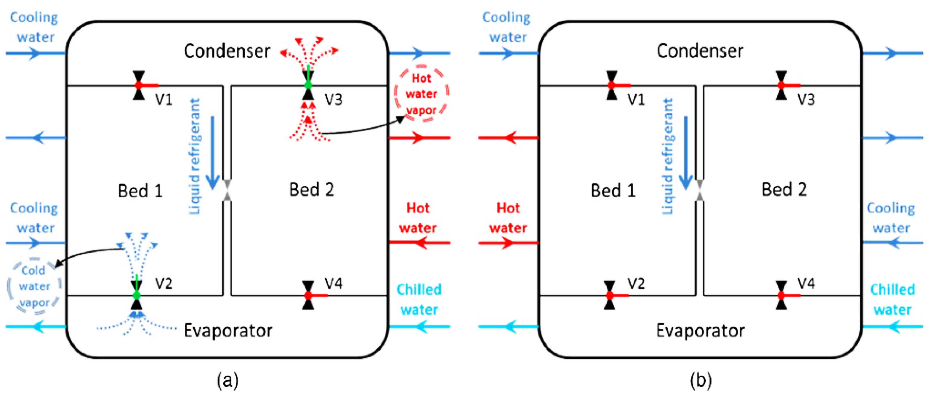
Figure 2.
Cone-shaped traps and antlions' hunting behaviour.
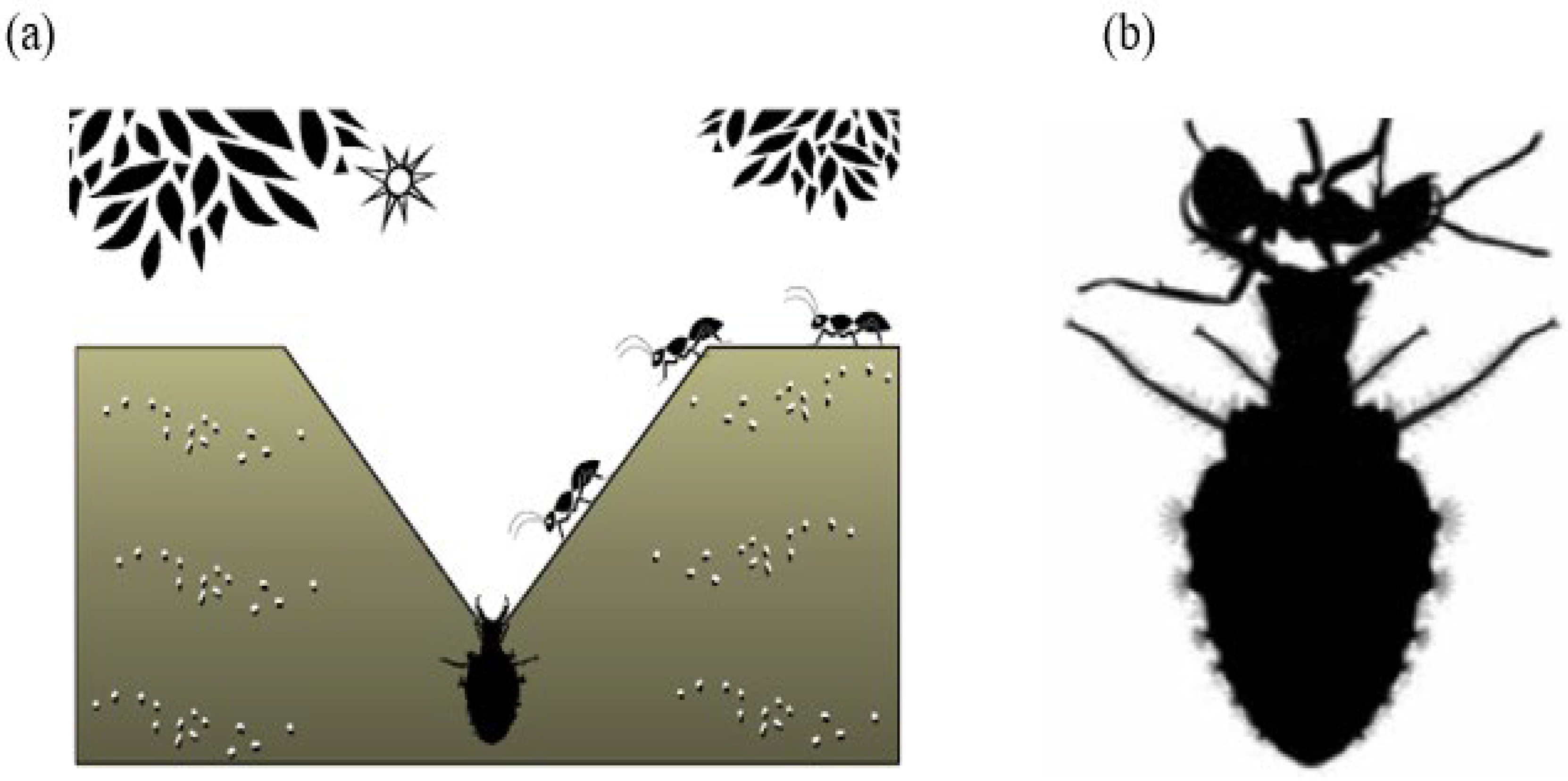
Figure 3.
An ant walking randomly inside an antlion’s trap.
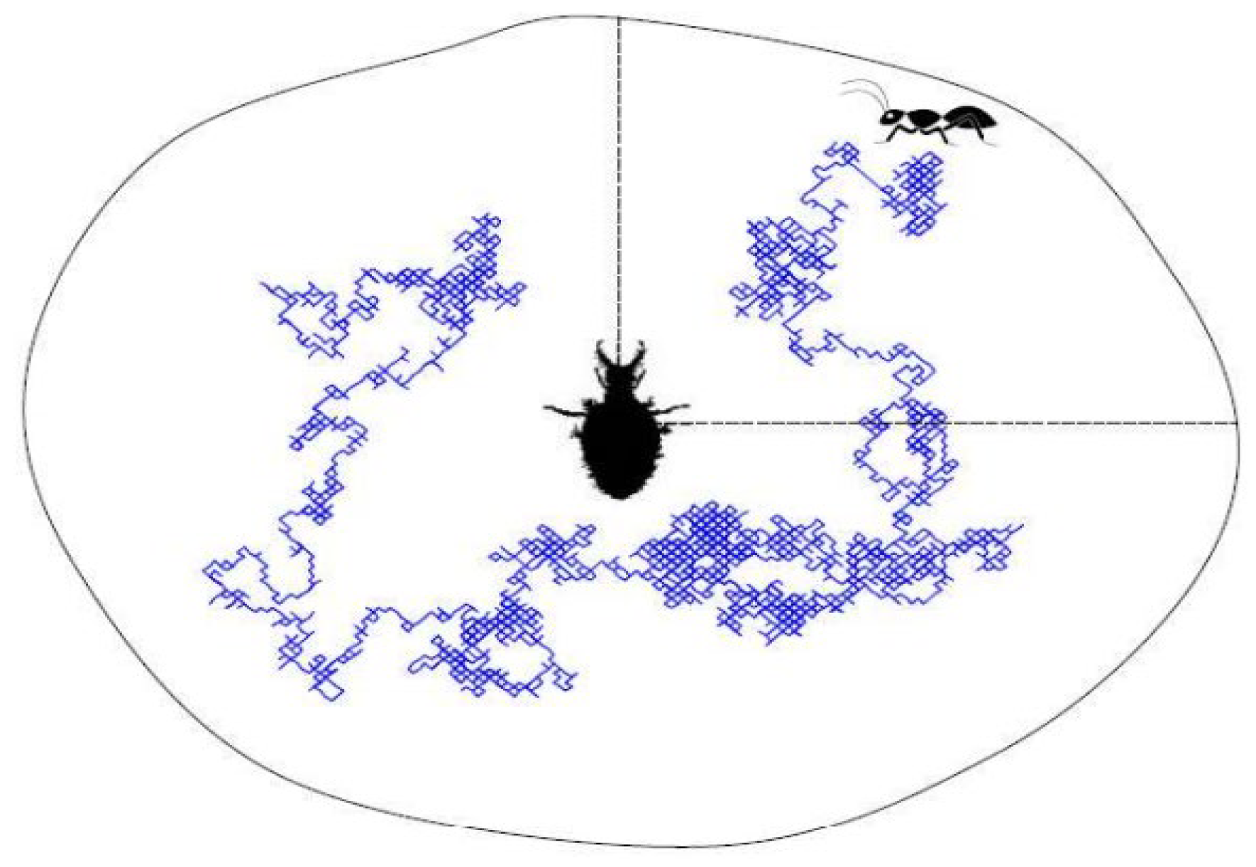
Figure 5.
Workflow of the Multi-Objective Ant Lion Optimizer (MOALO).
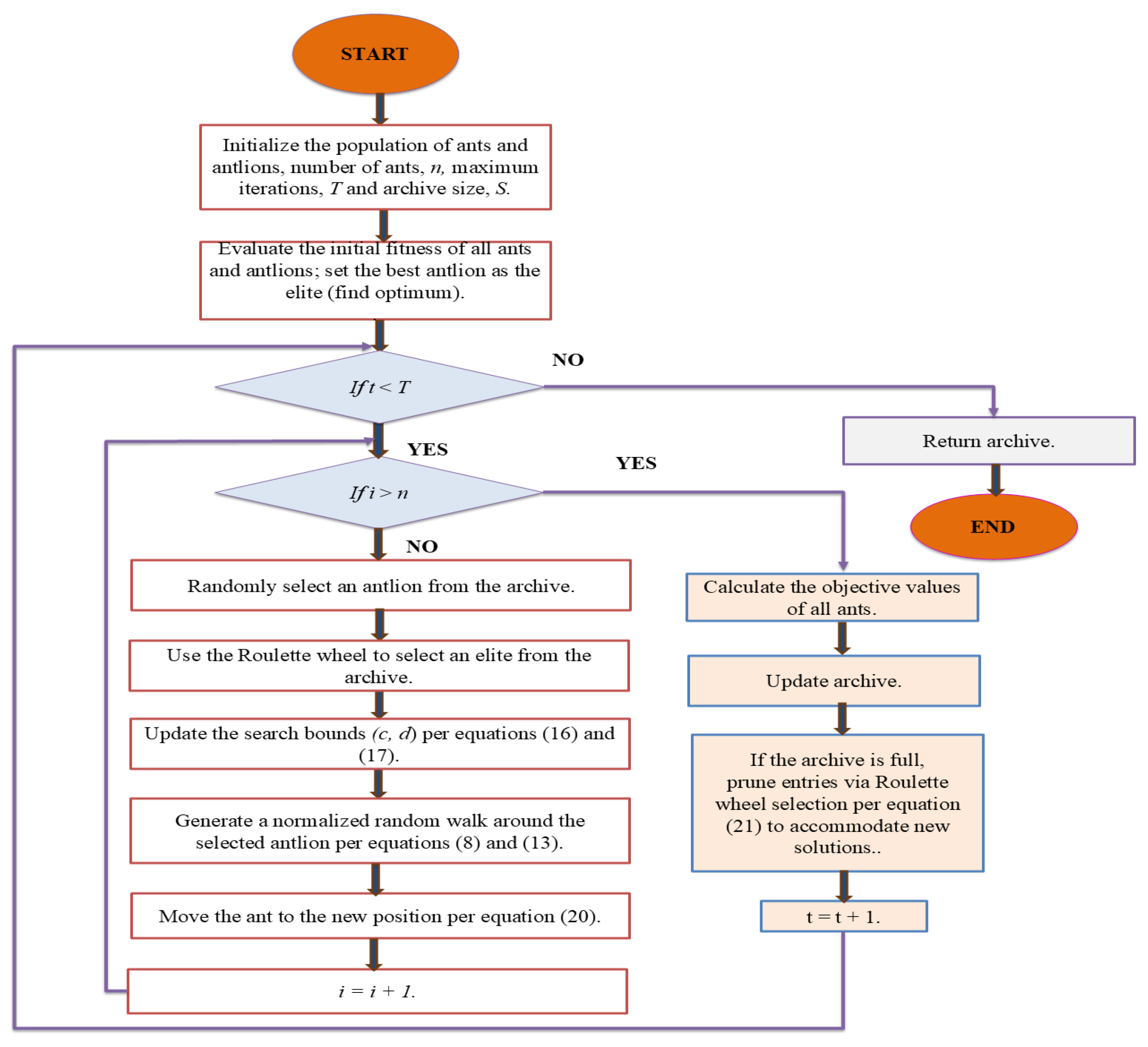
Figure 6.
Pairwise 2-D projections of the MOALO non-dominated set (N = 100). (a) COP versus ; (b) vs ; (c) COP vs
Figure 6.
Pairwise 2-D projections of the MOALO non-dominated set (N = 100). (a) COP versus ; (b) vs ; (c) COP vs
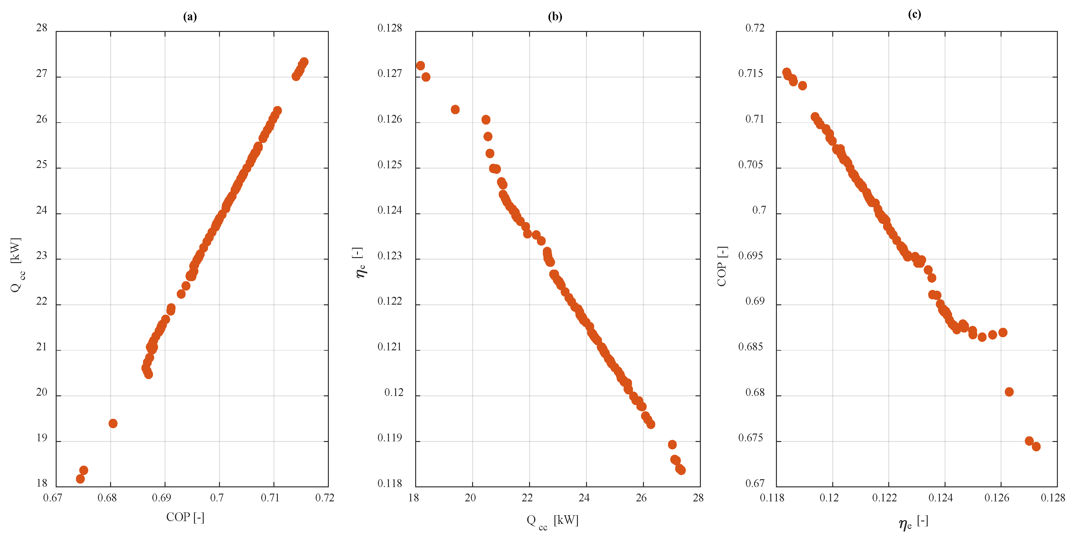
Figure 7.
Sensitivity of the Pareto set to hot-water inlet temperature, . Panels: (a) . versus COP; (b) versus COP; (c) versus .
Figure 7.
Sensitivity of the Pareto set to hot-water inlet temperature, . Panels: (a) . versus COP; (b) versus COP; (c) versus .
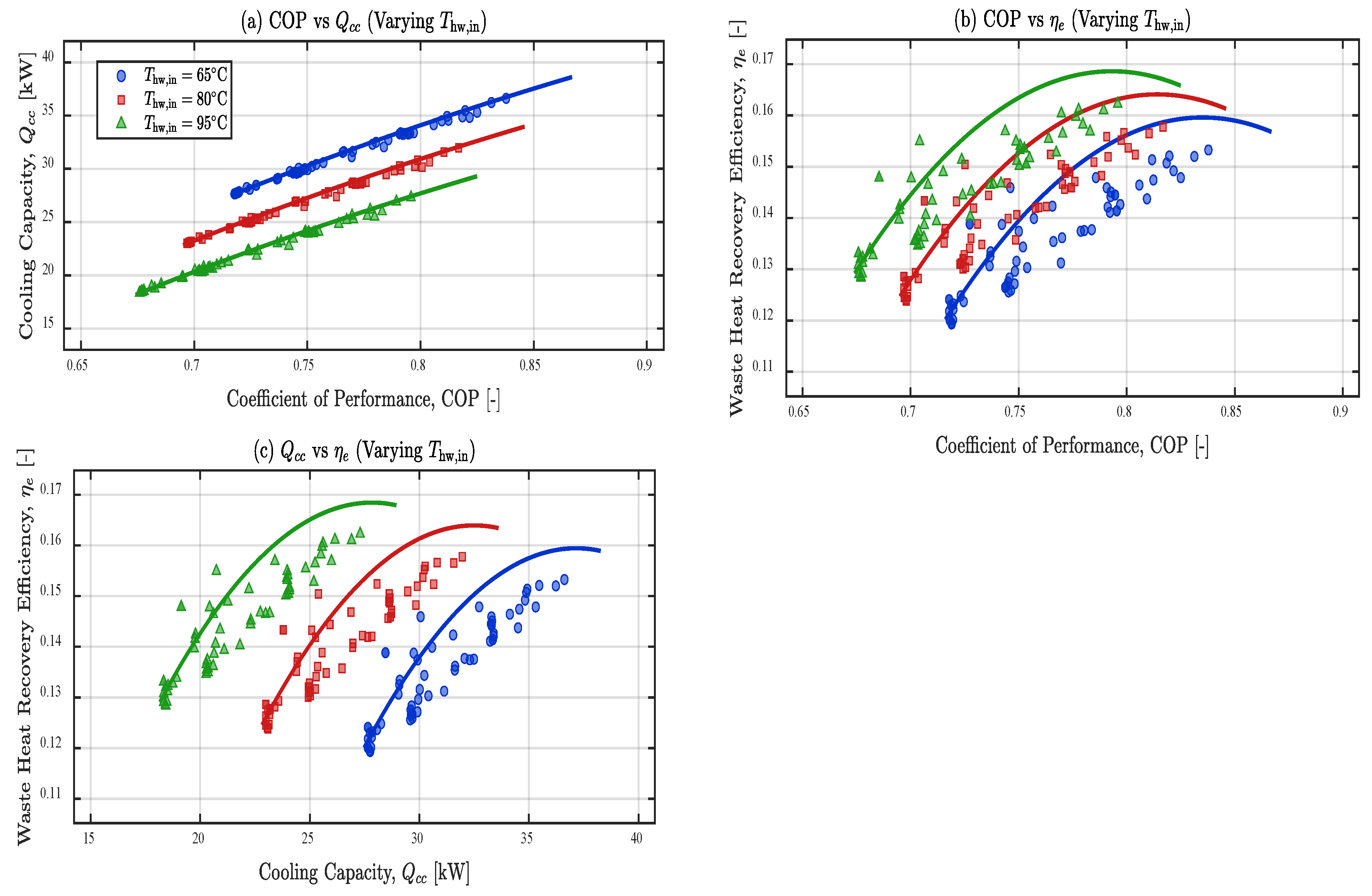
Figure 8.
Sensitivity of the Pareto set to cooling water inlet temperature, Panels: (a) versus COP; (b) versus COP; (c) versus .
Figure 8.
Sensitivity of the Pareto set to cooling water inlet temperature, Panels: (a) versus COP; (b) versus COP; (c) versus .
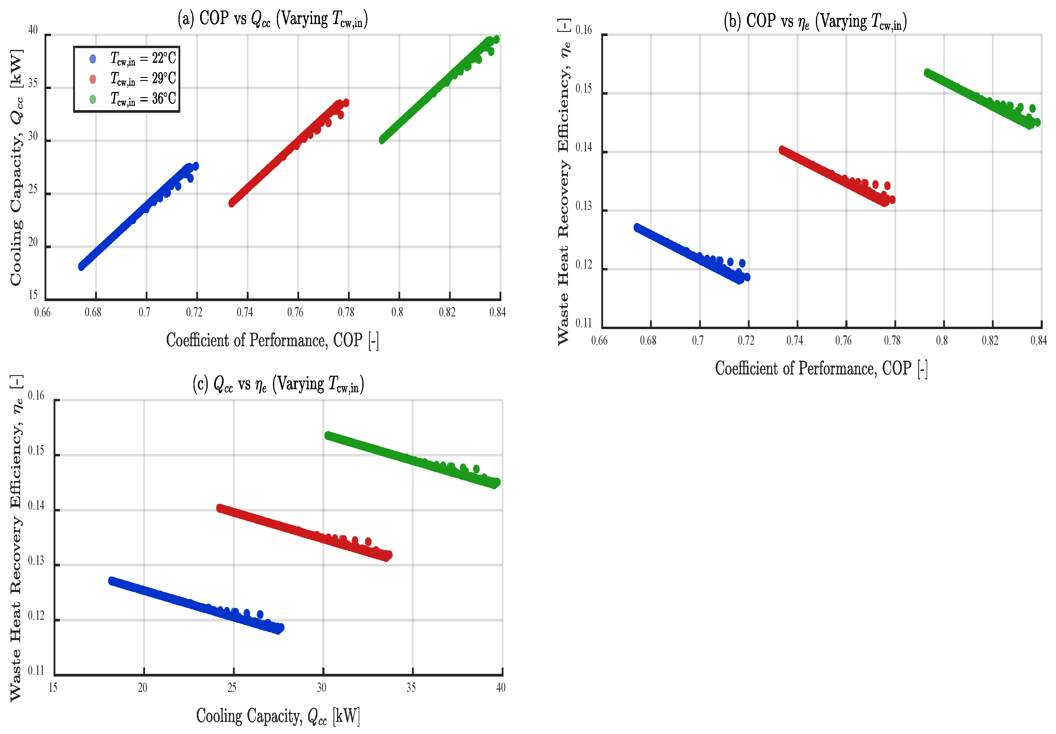
Figure 9.
Sensitivity of the Pareto set to cooling water inlet temperature, . Panels: (a) versus COP; (b) versus COP; (c) versus .
Figure 9.
Sensitivity of the Pareto set to cooling water inlet temperature, . Panels: (a) versus COP; (b) versus COP; (c) versus .
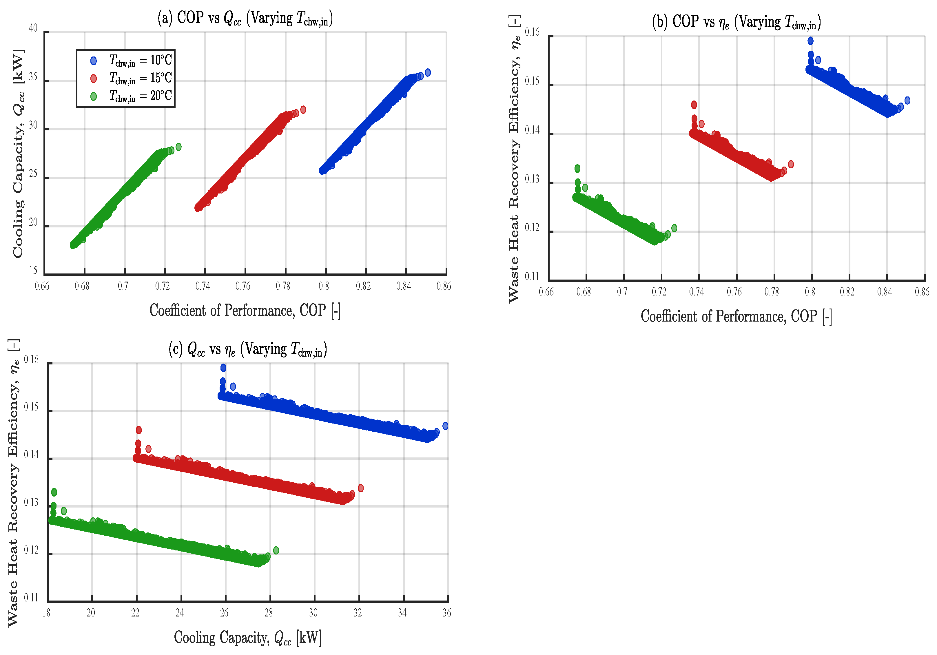
Figure 10.
Sensitivity of the Pareto set to cooling water inlet temperature, . Panels: (a) versus COP; (b) versus COP; (c) versus .
Figure 10.
Sensitivity of the Pareto set to cooling water inlet temperature, . Panels: (a) versus COP; (b) versus COP; (c) versus .
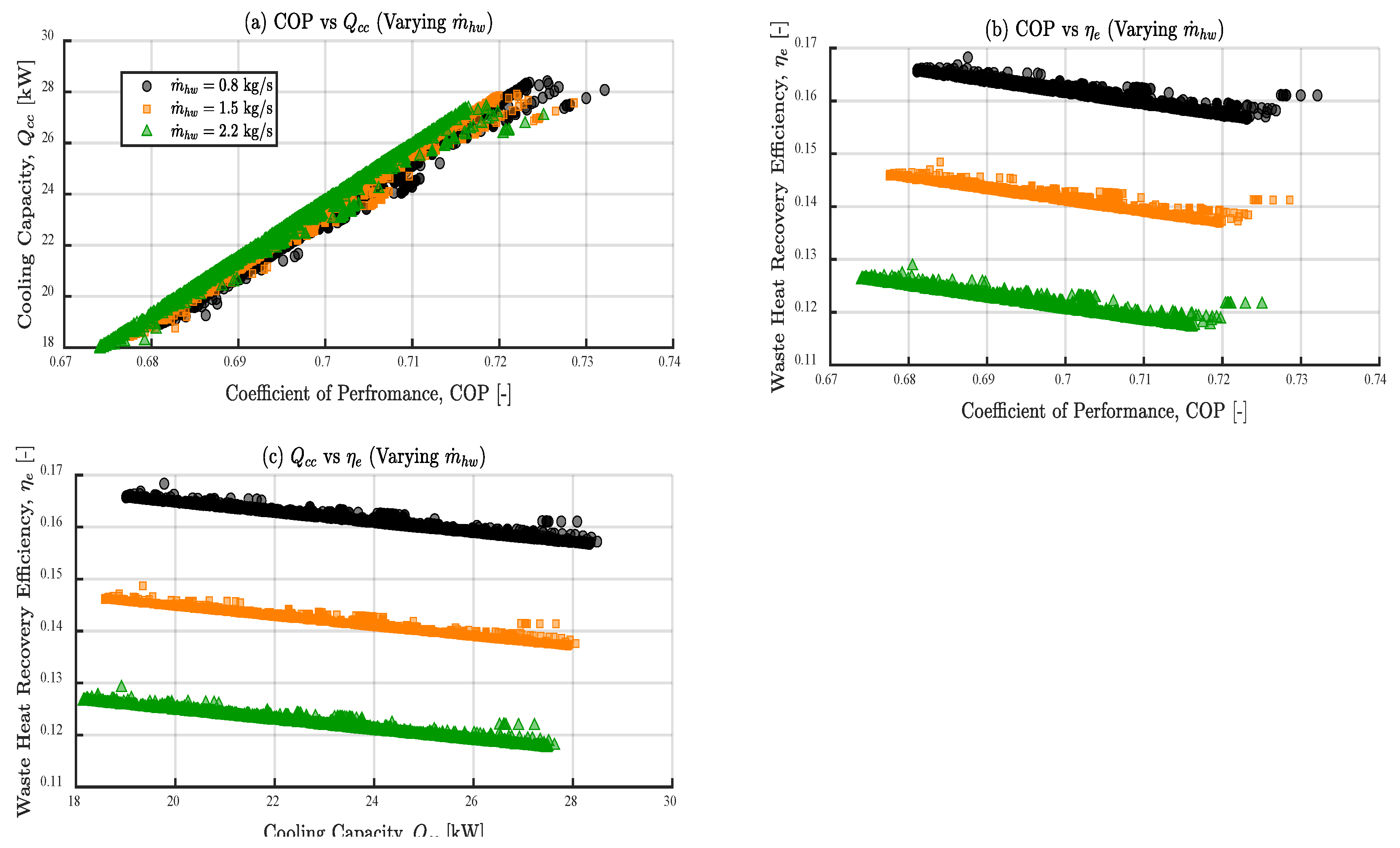
Figure 11.
Sensitivity of the Pareto set to cooling water inlet temperature, . Panels: (a) versus COP; (b) versus COP; (c) versus
Figure 11.
Sensitivity of the Pareto set to cooling water inlet temperature, . Panels: (a) versus COP; (b) versus COP; (c) versus
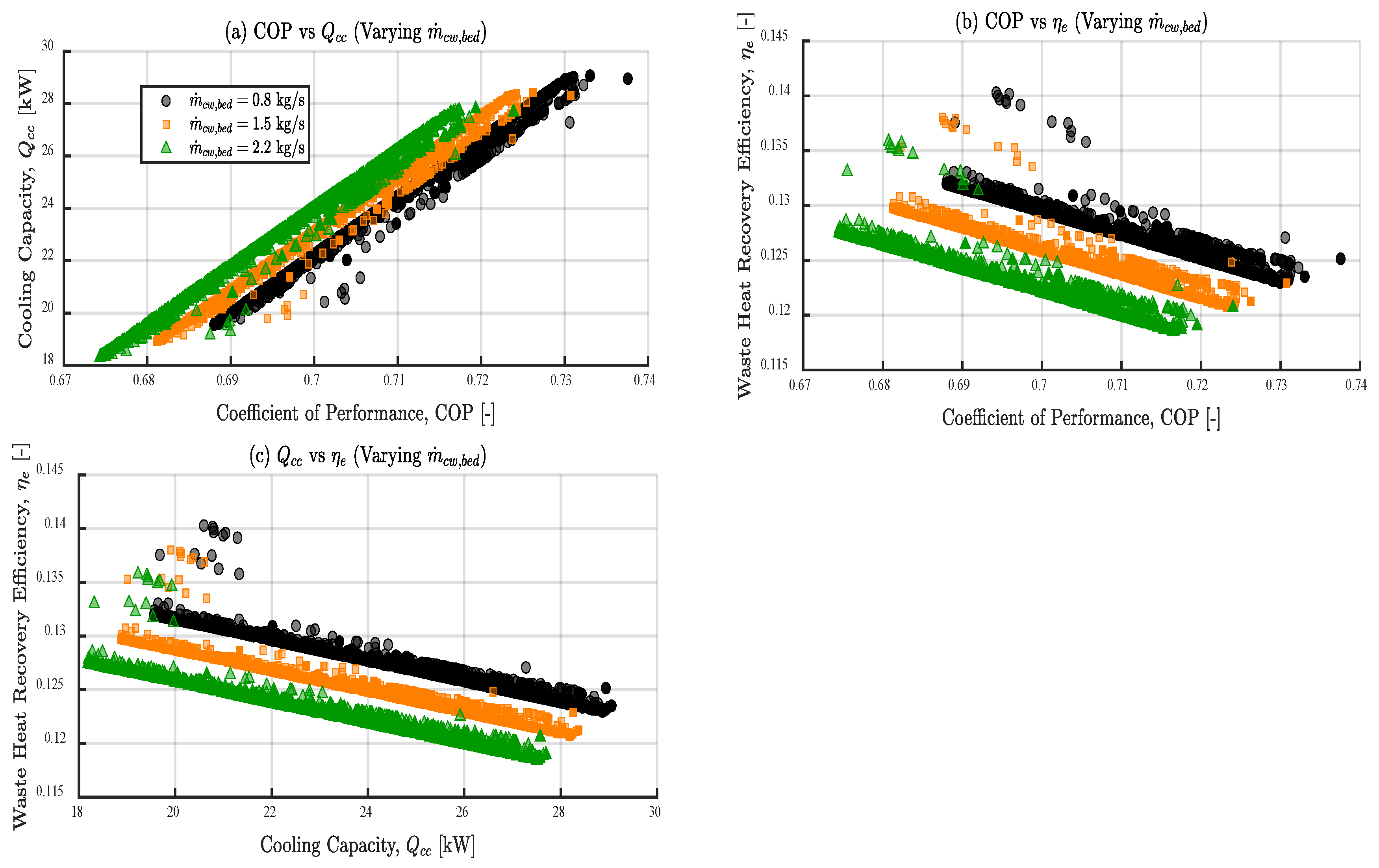
Figure 12.
Sensitivity of the Pareto set to chilling water mass flow, . Panels: (a) versus COP; (b) versus COP; (c) versus
Figure 12.
Sensitivity of the Pareto set to chilling water mass flow, . Panels: (a) versus COP; (b) versus COP; (c) versus
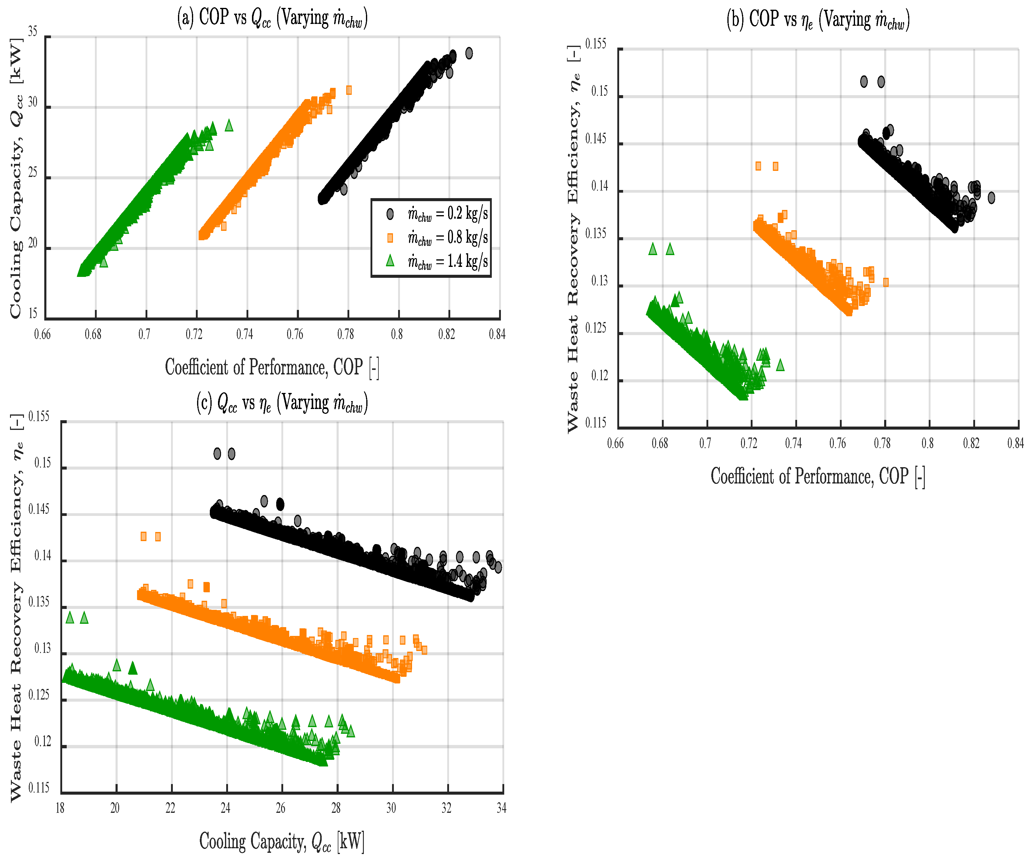
Figure 13.
Sensitivity of the Pareto set to condenser cooling water mass flow, . Panels: (a) versus COP; (b) versus COP; (c) versus
Figure 13.
Sensitivity of the Pareto set to condenser cooling water mass flow, . Panels: (a) versus COP; (b) versus COP; (c) versus
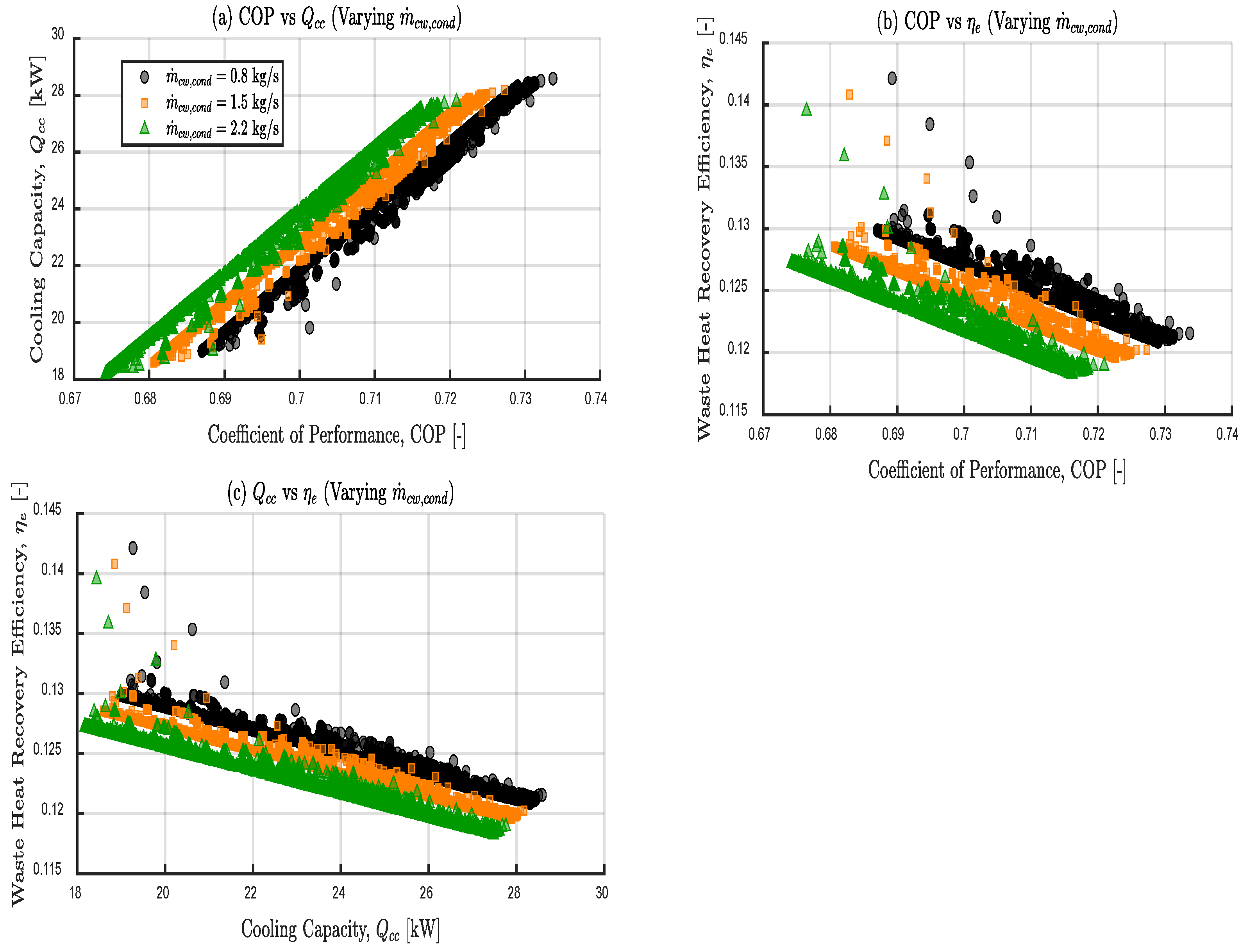
Figure 14.
Sensitivity of the Pareto set to bed overall conductance, Panels: (a) versus COP; (b) versus COP; (c) versus
Figure 14.
Sensitivity of the Pareto set to bed overall conductance, Panels: (a) versus COP; (b) versus COP; (c) versus
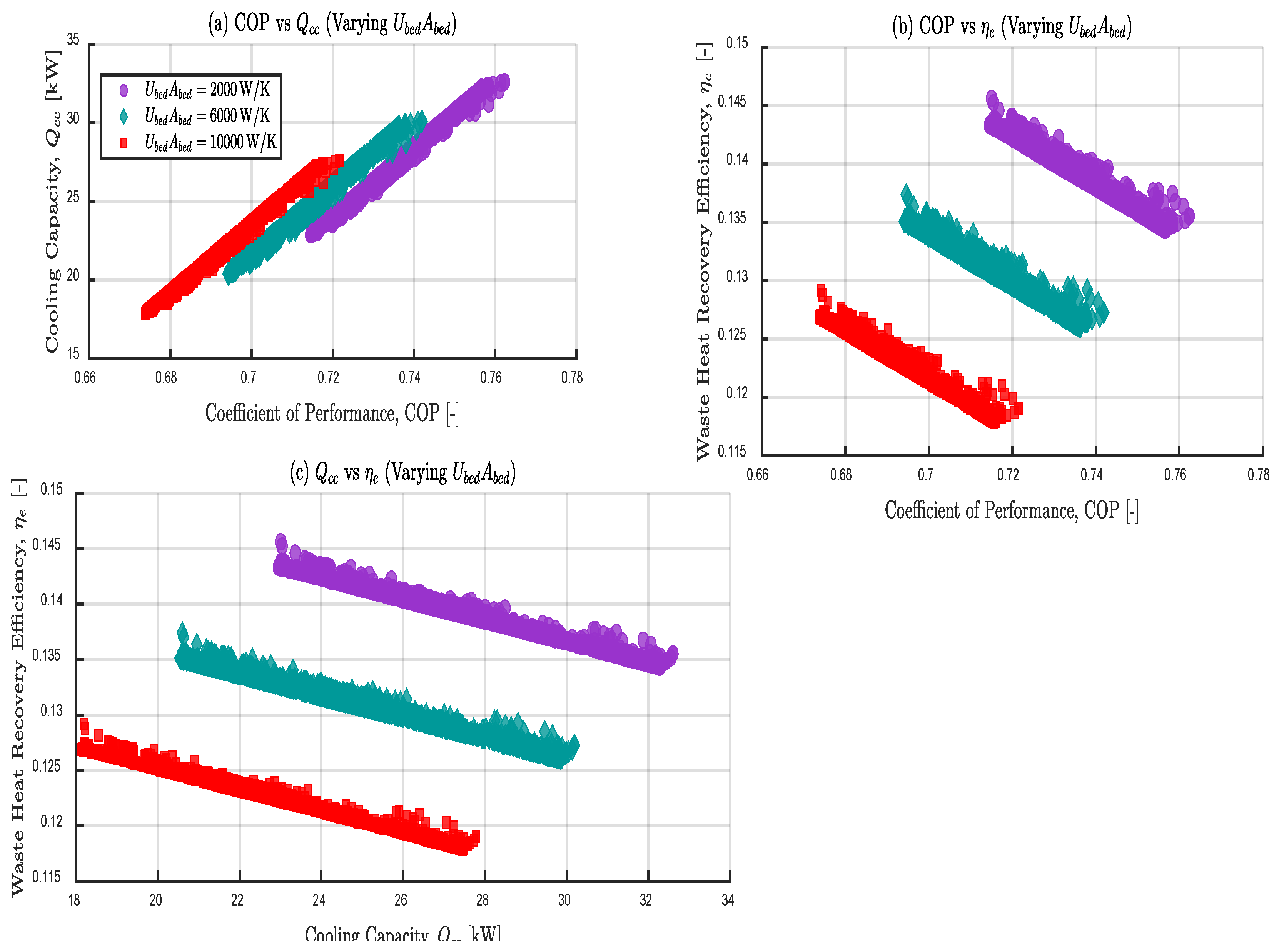
Figure 15.
Sensitivity of the Pareto set to condenser overall conductance,. Panels: (a) versus COP; (b) versus COP; (c)versus
Figure 15.
Sensitivity of the Pareto set to condenser overall conductance,. Panels: (a) versus COP; (b) versus COP; (c)versus
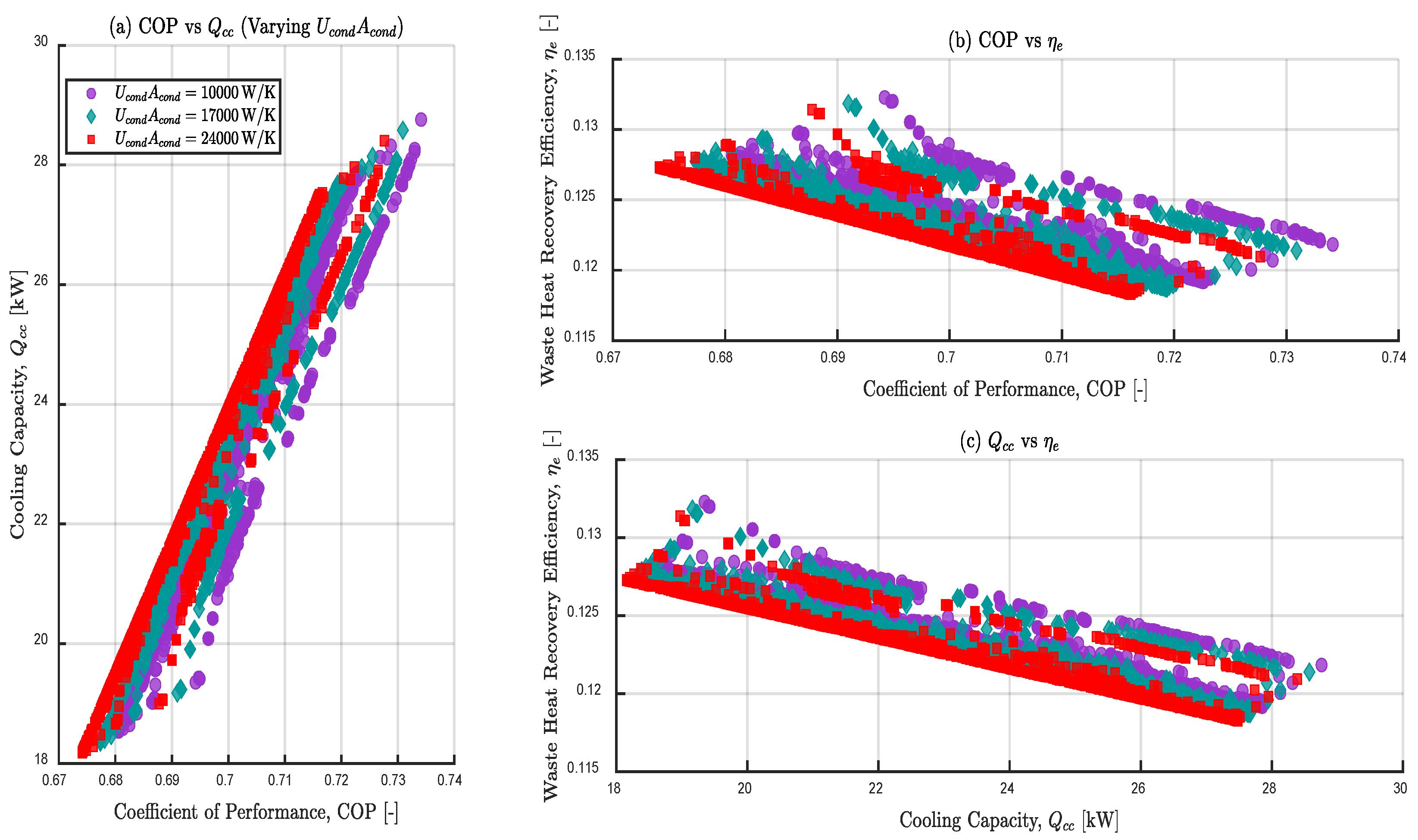
Figure 16.
Sensitivity of the Pareto set to evaporator overall conductance Panels: (a) versus COP; (b) versus COP; (c) versus
Figure 16.
Sensitivity of the Pareto set to evaporator overall conductance Panels: (a) versus COP; (b) versus COP; (c) versus
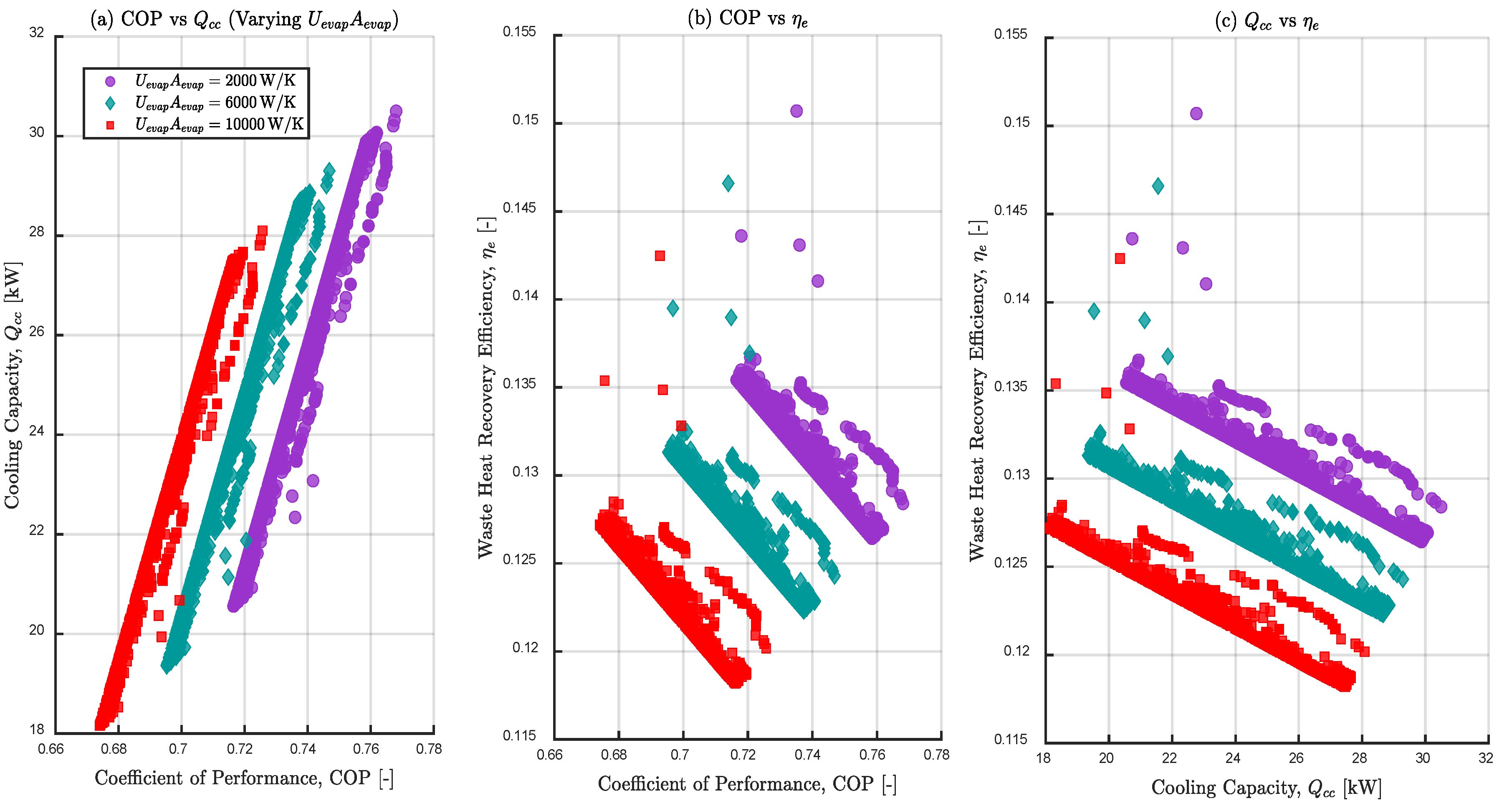
Table 1.
Decision variables and bounds.
| Variable Description | Symbol | Range | Units |
| Hot water inlet temperature | 65 – 95 | ◦C | |
| Cooling water inlet temperature | 22 – 36 | ◦C | |
| Chilled water inlet temperature | 10 – 20 | ◦C | |
| Hot water mass flow rate | 0.8 – 2.2 | kgs⁻¹ | |
| Bed cooling water mass flow rate | 0.8 – 2.2 | kgs⁻¹ | |
| Chilled water mass flow rate | 0.2 – 1.4 | kgs⁻¹ | |
| Condenser cooling water mass flow rate | 0.8 – 2.2 | kgs⁻¹ | |
| Adsorbent bed overall thermal conductance | 2,000 – 10,000 | W/K | |
| Evaporator overall thermal conductance | 2,000 – 10,000 | W/K | |
| Condenser overall thermal conductance | 10,000 – 24,000 | W/K |
Table 5.
Set values of the hyperparameters.
| Hyperparameter | Value |
| Maximum Number of Iterations | 100 |
| Population Size (Number of Ants) | 100 |
| Number of Antlions | 100 |
| Archive Size | 200 |
| Search Space Dimension | 10 |
| Maximum Number of Iterations | 100 |
Table 6.
Comparison of Literature benchmarks studies for single-stage silica-gel/water ADCs versus this study’s MOALO (This Work).
Table 6.
Comparison of Literature benchmarks studies for single-stage silica-gel/water ADCs versus this study’s MOALO (This Work).
| Parameter | Literature (Selected Anchors) | MOALO — This Work |
| COP range | Typical around 0.5–0.6 for single-stage silica-gel/water adsorption chillers; upper values ≤ 0.7 reported in manufacturer data [56,57] | Approximately 0.69–0.71 (Pareto set) |
| Laboratory or prototype report 2–10 kW [60]; product class 10 kW [57]; pilot/field 30–105 kW [58]; commercial 35–1180 kW [59] | Approximately 18–27.3 kW (Pareto set) | |
| Seldom reported explicitly in product literature and many system papers; emphasis typically on COP/capacity [61] | Approximately 0.118–0.1275 (11.8–12.75 %) | |
| Operating temperatures | Single-stage silica-gel/water, typical temperature drive 60–95 °C, reviewed chilled-water temperature ranges 10–20 °C [56] | Envelope: = 65–95 °C; ≈ 22 °C; ≈ 20 °C |
| System scale context | Commercial silica-gel/water ADCs span tens of kW to >1 MW (35–1180 kW line) [59] | This work falls in the low-commercial or high-pilot scale. |
Disclaimer/Publisher’s Note: The statements, opinions and data contained in all publications are solely those of the individual author(s) and contributor(s) and not of MDPI and/or the editor(s). MDPI and/or the editor(s) disclaim responsibility for any injury to people or property resulting from any ideas, methods, instructions or products referred to in the content. |
© 2025 by the authors. Licensee MDPI, Basel, Switzerland. This article is an open access article distributed under the terms and conditions of the Creative Commons Attribution (CC BY) license (http://creativecommons.org/licenses/by/4.0/).
Copyright: This open access article is published under a Creative Commons CC BY 4.0 license, which permit the free download, distribution, and reuse, provided that the author and preprint are cited in any reuse.


