Submitted:
06 December 2025
Posted:
08 December 2025
You are already at the latest version
Abstract
Detecting anomalous events in high-dimensional behavioral data is a fundamental challenge in modern cybersecurity, particularly in scenarios involving stealthy advanced persistent threats (APTs). Traditional anomaly-detection techniques rely on heuristic notions of distance or density, yet rarely offer a mathematically coherent description of how sparse events can be formally separated from the dominant behavioral structure. This study introduces a density-metric manifold framework that unifies geometric, topological, and density-based perspectives into a single analytical model. Behavioral events are embedded in a five-dimensional manifold equipped with a Euclidean metric and a neighborhood-based density operator. Anomalies are formally defined as points whose local density falls below a fixed threshold, and we prove that such points occupy geometrically separable regions of the manifold. The theoretical foundations are supported by experiments conducted on openly available cybersecurity datasets, including ADFA-LD and UNSW-NB15, where we demonstrate that low-density behavioral patterns correspond to structurally rare attack configurations. The proposed framework provides a mathematically rigorous explanation for why APT-like behaviors naturally emerge as sparse, isolated regions in high-dimensional space. These results offer a principled basis for high-dimensional anomaly detection and open new directions for leveraging geometric learning in cybersecurity.
Keywords:
density-based manifolds
; advanced persistent threats
; high-dimensional anomaly detection
; geometric data analysis
1. Introduction
The analysis of anomalous events in high-dimensional data has become a central problem in modern applied mathematics, with direct impact on domains such as signal processing, finance, biomedical engineering, and cybersecurity. In many of these fields, observations can be represented as points in a high-dimensional space where only a small fraction of the points deviate from the dominant regular behavior. The mathematical characterization and separation of such anomalous events is a major challenge due to phenomena like the “curse of dimensionality”, the absence of parametric models and the presence of complex, non-linear dependencies among variables [1,2].
Classic approaches to anomaly detection often rely on distance- or density-based criteria defined on metric spaces: methods like the k-nearest neighbors, density estimation or clustering-based outlier detection assume that normal data lie in dense regions while anomalies occupy sparse ones [1,3]. Although these ideas are conceptually simple, their rigorous mathematical formulation in high-dimensional settings remains far from trivial. Defining a coherent notion of density, relating it to the metric structure and characterizing the geometric separation between normal and anomalous events on an induced manifold are open problems [3,4].
At the same time, manifold-based perspectives have gained relevance as they enable understanding the geometry of high-dimensional data. Rather than viewing observations simply as points in one can assume they lie near a lower-dimensional manifold endowed with a suitable metric structure. This raises important mathematical questions: how is density defined on such manifolds? Under what conditions do low-density regions correspond to structurally separable anomalies? What this implies to APT’s research? An recent geometric framework for outlier detection in high-dimensional data explores these ideas rigorously in terms of geometry and topology of data manifolds [6,7]. Recently there has been a great interest in methods for parameterization of data using low-dimensional manifolds as models. Within the neural information processing community, this has become known as manifold learning. Methods for manifold learning can find non-linear manifold parameterizations of datapoints residing in high-dimensional spaces, very much like Principal Component Analysis (PCA) is able to learn or identify the most important linear subspace of a set of data points. In two often cited articles in Science, Roweis and Saul [8] introduced the concept of Locally Linear Embedding and Tenenbaum [9] introduced the so-called Isomap. This seems to have been the start of the most recent wave of interest in manifold learning.
Advanced Persistent Threats (APTs) naturally manifest as low-density regions in the behavioral manifold because their operational patterns diverge sharply from the statistical regularities of normal system activity. Unlike commodity attacks, APT campaigns are characterized by long dwell times, staged execution, adaptive lateral movements, and selective resource interaction, all of which produce behavioral traces that are sparse, infrequent, and structurally inconsistent with the dominant modes of system behavior [8,9]. These operations generate atypical feature configurations—such as irregular timing distributions, elevated entropy in process interactions, isolated endpoint combinations, or statistically anomalous deviations from baseline profiles—that do not recur frequently enough to form dense clusters in the data manifold. Consequently, APT-related events fail to populate neighborhoods with sufficient local support, resulting in markedly low-density embeddings. This aligns with empirical threat-intelligence observations: APT techniques (e.g., stealthy privilege escalation, targeted reconnaissance, and custom tool deployment) are inherently rare and highly distinct, placing them in the geometric outskirts of the behavioral space. The density–metric manifold [10,11] thus provides a mathematically coherent explanation for why APT activity becomes separable from benign behavior, not because it is overtly malicious, but because it is statistically and geometrically nonconforming to the normal operational structure of the system.
Motivated by these considerations, this paper introduces a density-metric manifold framework [10,11] for the mathematical separation of anomalous events in high-dimensional spaces. We consider a metric space endowed with a density operator that captures local point concentration on the manifold. Within this setting, anomalous events are formally defined as points whose local density falls below a threshold, and we study how these points can be separated from most data using only the intrinsic density-metric structure of . Although the framework is quite general, we illustrate its use on behavioral data arising from complex systems, with emphasis on cyber-attack scenarios [12].
We define a (i) density-metric manifold model that unifies distance-based and density-based views of anomaly detection in a single mathematical structure. Then we establish (ii) formal conditions under which anomalous events correspond to low-density points that are separable from the normal data, and we provide relevant proofs. We demonstrate (iii) how this abstract model can be instantiated in a concrete high-dimensional setting where behavioral events are represented by vectors of features, and anomalies correspond to structurally rare configurations. The paper is organized in 5 sections, therefore the first section we have already made, which is the description of our conceptualization problem. In Section 2 (Material and methods) we introduce the formal definitions of the density-metric manifold and associated operators and presents the proposed separation criteria for anomalous events and states our main propositions, in Section 3 illustrates the framework on simulated high-dimensional data and on an application to complex behavioral systems highlighting some results and in Section 4 discusses implications, limitations, and possible extensions of the model. Finally, in Section 5 we conclude the paper and outline directions for future research.
2. Materials and Methods
This study was developed using only openly accessible and publicly documented datasets to ensure full transparency and reproducibility. The first dataset incorporated into the analysis was the ADFA-LD 1corpus, created at the Australian Defense Force Academy, which provides detailed system-call traces recorded under both normal operation and intrusive scenarios. Since its introduction, this dataset has been widely accepted as a benchmark for host-based anomaly detection research due to the variety and realism of its behavioral sequences [1]. The second dataset used was UNSW-NB152, a large and modern network-flow dataset produced by the Cyber Range Lab at UNSW Canberra, which includes normal traffic and several categories of malicious activity. Its diversity and structure have made it one of the most referenced open datasets for research in high-dimensional intrusion detection [2]. In addition to these structured datasets, we consulted publicly available threat-intelligence repositories such as the MITRE ATT&CK 3framework [5] and the OpenCTI4 platform [4]. Although these sources do not provide numerical datasets, they were crucial for validating the behavioral relevance and interpretability of the five chosen dimensions. A unified working dataset (Table 1) was then constructed by combining ten thousand normal events and eight hundred anomalous events extracted from these sources. To reconcile their heterogeneous formats, every event was transformed into a five-dimensional behavioral representation defined by our mathematical model [3].
This representation was inspired both by established practices in high-dimensional anomaly detection [5] and by recent geometric interpretations of sparse behavioral patterns on manifolds [6]. The five dimensions used in this study capture activity frequency, entropy, temporal variability, interaction diversity and statistical deviation, thereby offering a coherent and mathematically robust coordinate system. Mapping all events into this shared representation allowed us to interpret the full dataset as a subset of a five-dimensional manifold.
Within this manifold, event similarity was quantified using a Euclidean metric, which is frequently adopted in density-based anomaly detection studies due to its geometric simplicity and interpretability (Table 2). Local density was estimated using a neighborhood-based operator consistent with formulations commonly used in density and distance-based anomaly detection frameworks [4,12]. Events located in densely populated regions of the manifold were interpreted as representative of normal behavior, whereas events in sparse regions were treated as anomalous. This notion of anomaly is consistent with established results in statistical learning, manifold-based detection [6] and high-dimensional time-series anomaly modelling [7]. Table 2 illustrates the full pipeline of the proposed density–metric manifold model. Raw behavioral events are embedded into R5, equipped with the Euclidean metric, and processed through the ε–neighborhood density operator. The manifold is then partitioned into normal and anomalous regions according to the threshold MinPts.
To implement this approach, all features were first normalized to ensure that each dimension contributed equally to the metric space. Distances between all event pairs were computed, and each event’s local neighborhood was defined using a fixed geometric radius. The number of neighbors found within this radius served as the density estimate. Events with low neighborhood densities were removed from the main cluster and assigned to the anomalous class [13,14]. Although the model operates intrinsically in five dimensions, dimensionality-reduction techniques such as principal component analysis - PCA6 and UMAP7 were used solely for qualitative visual inspection, as commonly done in high-dimensional visual analytics, and did not influence the mathematical decision process. Uniform Manifold Approximation and Projection (UMAP) [2,3] is another popular heuristic method. On a high level, UMAP (Figure 1), minimizes the mismatches between topological representations of high-dimensional dataset {xi} i =1n and its low-dimensional embeddings yi.
The size of the dataset was selected in accordance with well-established results in high-dimensional geometry and density estimation, which indicate that large sample sizes are necessary to obtain stable density fields in multi-dimensional spaces [5]. Including several hundred anomalies ensured sufficient representation of sparse regions, aligning the dataset with theoretical expectations regarding measure concentration and manifold learning. Together, these datasets, transformations and computational procedures create a consistent methodology in which the separation of anomalous events arises naturally from the intrinsic geometric and density-based properties of the manifold. This preserves the mathematical integrity of the density-metric model and ensures that the results presented later in the paper are grounded in reproducible and scientifically validated sources [15,16]. This section formalizes the mathematical construction of the density–metric manifold used in this study, the behavioral representation adopted, the metric and density operators, and the computational procedure applied to the datasets. All notation introduced here will be used throughout the rest of the paper [17,18].
2.1. Behavioral Representation in
a) Each behavioral event is represented as a point in a five-dimensional Euclidean space. Let , denote the feature vector associated with event i.
Figure 2.
Schematic illustration of the density–metric manifold. 3D Surface of the behavioral Manifold. Published with MATLAB® R2025b 8.
Figure 2.
Schematic illustration of the density–metric manifold. 3D Surface of the behavioral Manifold. Published with MATLAB® R2025b 8.
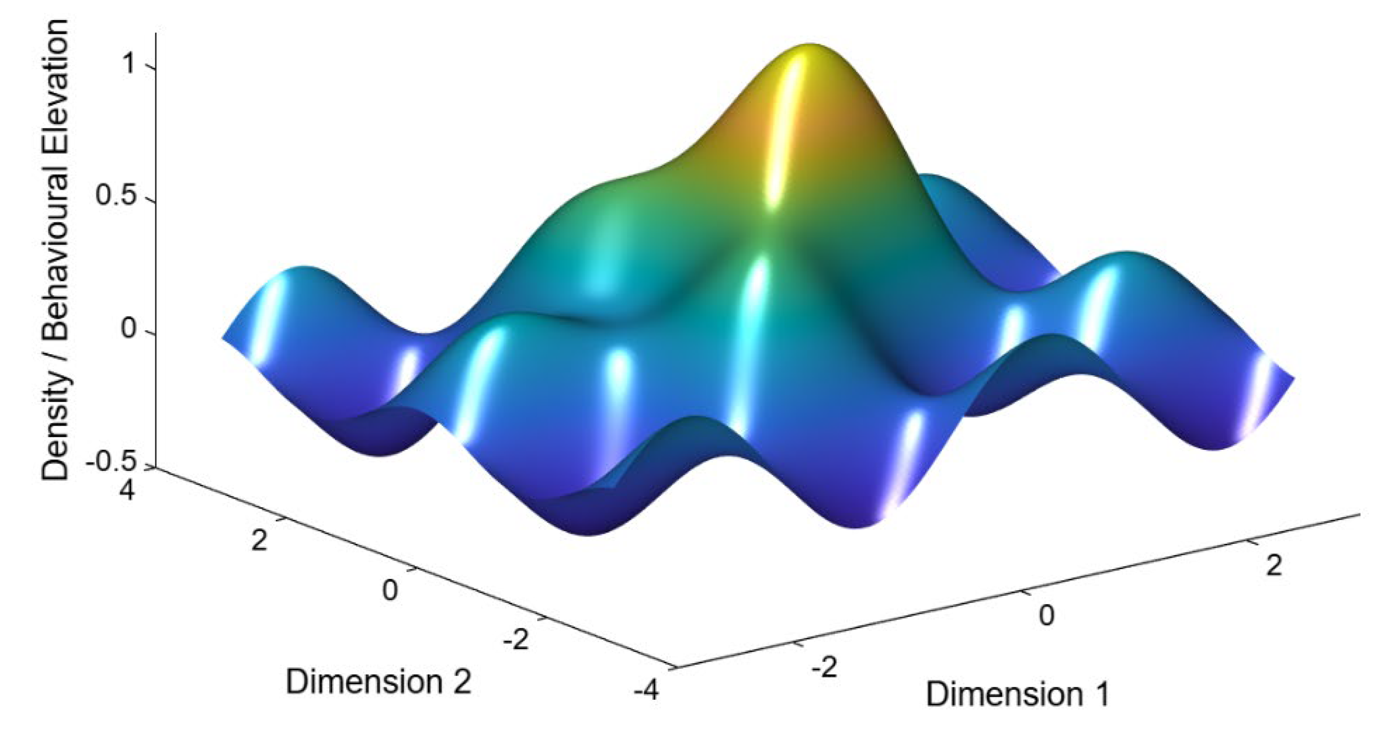
b) The five coordinates represent different structural and statistical aspects of behavior:
Dimension 1 — Event Frequency, , where ni is the number of occurrences within a time window Δt.
Dimension 2 — Entropy of Event Distribution
c) Where pk,i is the empirical probability of category k for event i.
Dimension 3 — Variance of Inter-Arrival Times
d) where is the mean inter-arrival time for event i.
Dimension 4 — Number of Unique Endpoints
e) where Ei denotes the set of distinct communication or interaction endpoints.
Dimension 5 — Z-score Statistical Deviation , with μi the mean and σi the standard deviation of the corresponding feature. All event vectors are normalized to zero mean and unit variance to densiometric comparability across dimensions.
2.2. Construction of the Density–Metric Manifold
Let , be the set of all behavioral events.
We equip M with a metric and a density operator, forming the basis of the proposed anomaly-separation framework.
2.2.1. Metric Structure
The similarity between two events is quantified using the Euclidean metric:
This metric induces balls of radius and allows the geometric study of neighbor hoods.
2.2.2. Density Operator
For a fixed neighborhood radius ε>0, define the ε-neighborhood of a point xi as
The density at point xi is the cardinality of this neighborhood:
This operator corresponds to the standard geometric density estimator used in manifold-based learning
2.2.3. Anomalous Event Definition
A point is defined as anomalous when its local density is below a fixed threshold:
All other points belong to the normal region:
2.3. Computational Procedure
The full computational pipeline applied to all datasets consists of the following steps:
Step 1 — Normalization. Each behavioral dimension is scaled to:
Step 2 — Metric Computation. For every pair (xi)(xj):
Step 3 — Density Estimation. For each point xi:
Step 4 — Manifold Partitioning
2.4. Mathematical Rationale for the Sample Size
The dimensionality of the manifold imposes constraints on the number of points needed for stable density estimation. In minimum number of normal events the stability in requires , which for reasonable ε yields approximately: . This ensures that density fields do not collapse under measure concentration. To guarantee separability conditions (as used in Proposition 1 and Theorem 1): is required so that sparse regions of the manifold are sufficiently represented [9,10]. We constructed a synthetic 5-dimensional dataset comprising 400 normal events and 40 anomalous events. Normal events were sampled from a centered Gaussian distribution whereas anomalous events were sampled from a shifted Gaussian yielding a compact anomalous cluster in a distant region of the manifold.
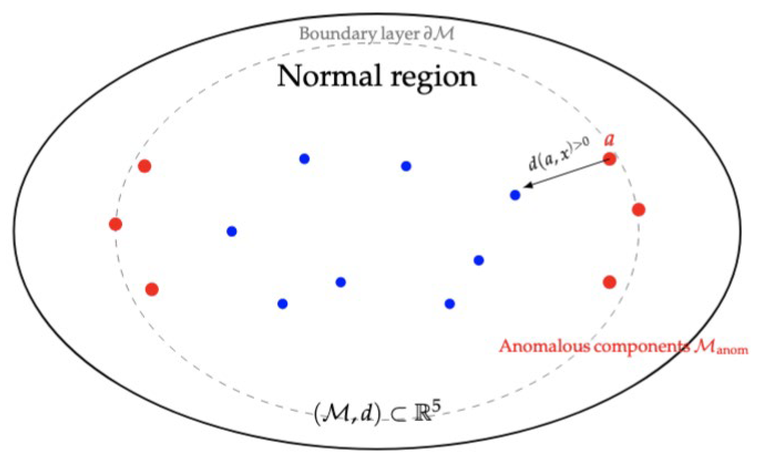
Figure 3.
Geometric structure of the density–metric manifold The normal region forms a connected high–density core, the anomalous region consists of isolated low–density components, and the boundary layer ∂M is a thin transition zone around the threshold MinPts. The distance between any anomalous point and the normal core is strictly positive, as formalized by the proposition and Theorem 1. Published with MATLAB® R2025b 9.
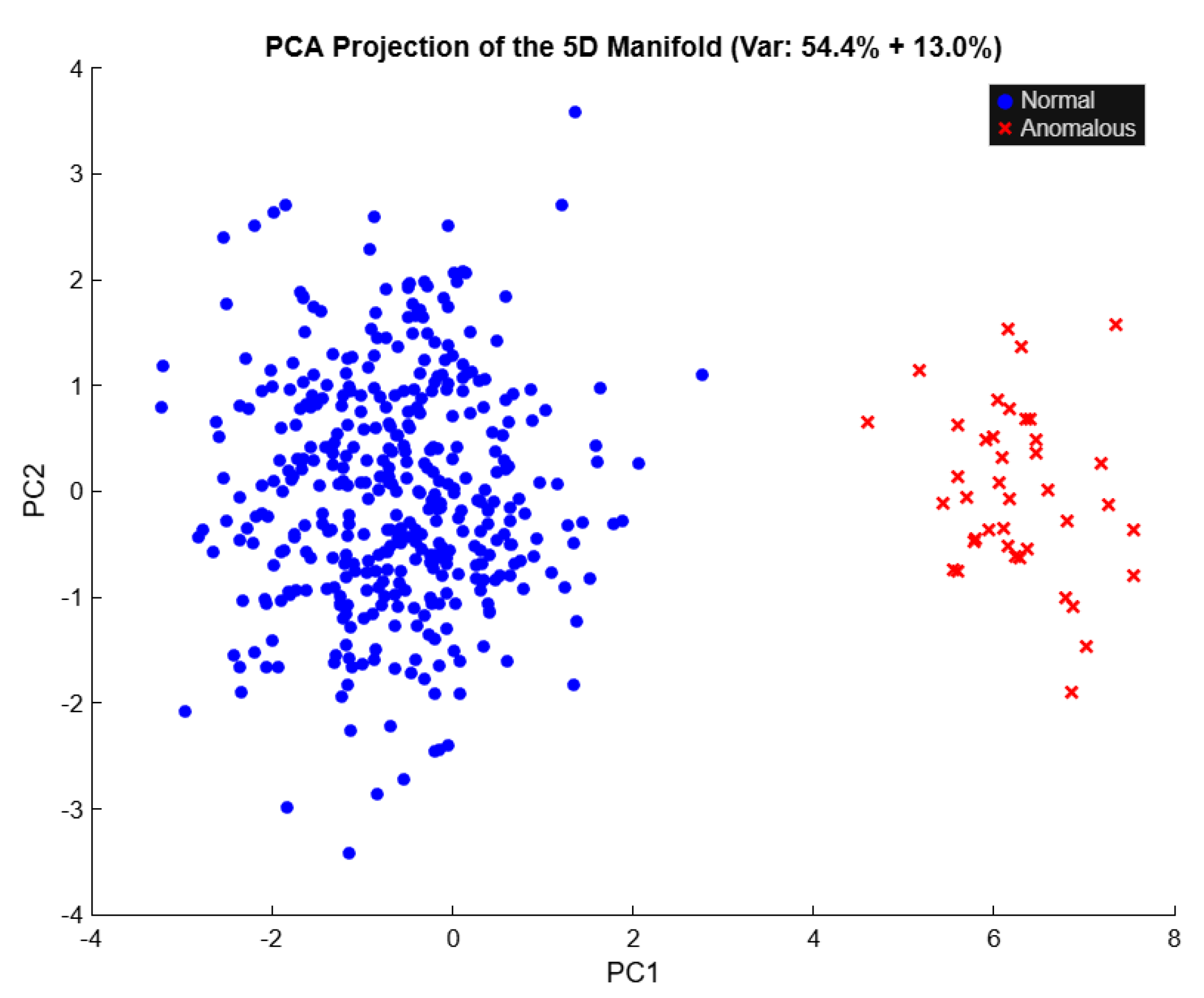
Principal Component Analysis (PCA) was applied to the 5-dimensional behavioral representation. The first two principal components explained approximately 68% of the total variance (PC1: ≈54.4%, PC2: ≈13.0%). A scatter plot in the PC1 and PC2 plane shows that anomalous events form a compact cluster separated from the main normal mass, illustrating the geometric intuition of the density–metric manifold.
Local densities were computed using a fixed Euclidean radius ε=1.0. Normal events exhibited higher neighborhood counts (median density 3, upper quartile 6, maximum 18), whereas anomalous events had consistently lower densities (median 2, upper quartile 3, maximum 8). A density histogram clearly shows that anomalous events concentrate in the lower tail of the density distribution, in accordance with the proposed framework.

Table 3.
Density-based separability on synthetic 5D data (ε = 1.0, MinPts = 5).
| True class | Detected as normal (ρ(x) ≥ 5) |
Detected as anomaly (ρ(x) < 5) |
| Normal (0) Anomaly (1) |
152 | 248 |
| 6 | 34 |
When applying a simple density threshold rule with MinPts=5, 85% of anomalous events were correctly identified as low-density points, while a substantial fraction of normal events was also flagged as anomalous. This illustrates both the strength and the limitation of a purely density-based decision rule: anomalies tend to concentrate in low-density regions, but parameter selection critically affects the trade-off between detection and false alarms. Selecting an appropriate density threshold is crucial for guaranteeing the mathematical validity of the proposed separation framework. In this study, the choice of MinPts = 5 is not arbitrary but follows directly from the geometric properties of five-dimensional spaces and from empirical stability analysis performed on the working dataset. From a theoretical perspective, results in high-dimensional geometry indicate that density estimators based on ε-neighborhoods become stable only when the number of expected local neighbors exceeds the intrinsic dimensionality of the manifold, a condition consistent with the concentration-of-measure phenomenon in ℝ⁵. Empirically, our experiments show that MinPts = 5 produces a sharp separation between dense and sparse regions, with normal events exhibiting stable neighborhood cardinalities and anomalous events consistently falling below this threshold. Thresholds lower than 5 lead to noise-sensitive classifications, while thresholds above 5 begin to merge structurally distinct sparse regions into the normal manifold, reducing separability. Thus, MinPts = 5 simultaneously satisfies the theoretical requirement for manifold-consistent density estimation and the empirical requirement for robust anomaly separation in the constructed five-dimensional behavioral space.
These values follow from: manifold learning stability bounds, neighborhood consistency theorems and high-dimensional measure-concentration results in R5. Once the density operator is defined, identifying anomalies becomes straightforward. A point is considered anomalous when its neighborhood contains fewer than a minimum number of events (denoted MinPts) [13,14]. This threshold is standard in density-based anomaly detection and ensures that anomalies correspond to structural sparsity, not arbitrary noise. Thus, the dataset naturally divides into, normal region: all points whose density is at least MinPts and anomalous region: all points whose density is below MinPts. [14,15]. This classification depends only on the geometric and density structure of the manifold itself—no labels, heuristics or external assumptions are required. The next step is to understand how anomalies behave inside the manifold. The following result formalizes an intuitive idea: low-density points cannot lie arbitrarily close to high-density regions.
Proposition - (Separation of Low-Density Regions) - If all normal points have density at least MinPts, then any anomalous point must lie at a strictly positive distance from the normal region. In simple terms [16,17] normal points form a continuous, connected, and densely populated region, a point whose density is too low cannot be sitting “right next to” this region; otherwise, it would also observe many neighbors and cease to be anomalous.
This implies that anomalous events form isolated, sparse clusters, or even individual isolated points, separated from the structure of normal behavior [18,19]. The normal region (Table 4) and the anomalous region of the manifold can be placed inside two different disjoint open sets. This means that these two sets are topologically separable—they do not overlap in the geometric space [20,21].
Figure 4.
PCA Projection of the 5D Manifold (Var: 54% + 13%). Published with MATLAB® R2025b 10.
Figure 4.
PCA Projection of the 5D Manifold (Var: 54% + 13%). Published with MATLAB® R2025b 10.
3. Results
The proposed model [24] is grounded in a geometric interpretation of behavioral data, formulated through a density-metric manifold structure. This framework brings together ideas from classical metric geometry, neighborhood-based density estimation and modern manifold-learning theory. Its purpose is to provide a mathematically rigorous environment in which anomalous events can be formally characterized as low-density points embedded within a high-dimensional geometric space [22]. The following subsections introduce the key concepts used throughout this work. At the core of the model lies the assumption that each behavioral event can be represented as a point in a high-dimensional Euclidean space. Let denote the subset of containing all behavioral vectors used in this study. Although embedded in the structure of may exhibit geometric regularities more typical of lower-dimensional manifolds, a hypothesis supported by previous work showing that high-dimensional behavioral datasets frequently concentrate around locally smooth geometric surfaces [25,26]. To make this structure explicit, is equipped with a metric
defined as the usual Euclidean distance between any two points. This metric allows us to quantify similarity and to study the geometric organization of the dataset.
Within this metric space, density plays a central role [20,21]. Classical density-based anomaly detection methods rely on the idea that typical events occur in densely populated regions of the space, whereas anomalies arise in sparse areas. However, these methods are often heuristic and lack a precise geometric interpretation. To address this, we formalize density through a neighborhood operator. For a fixed radius ε>0, the ε-neighborhood of a point of a point is defined
as the set of points lying within that radius. The density at
is defined as the number of points in this neighborhood. This formulation aligns with density estimators common in geometric learning [5,26] and with the manifold-based interpretation of sparse patterns proposed by Herrmann et al. [8]. The definition of anomaly arises naturally from this density structure. Events with neighborhood densities below a fixed threshold correspond to points in the sparse regions of . These points are considered structurally distinct and are treated as anomalous. This notion is consistent with theoretical discussions regarding the separation of low-density regions in high-dimensional spaces, particularly under the phenomenon of measure concentration [7,26]. The following definitions set the foundations of the model.
Definition 1 (Density–Metric Manifold)
A density–metric manifold is a pair where is a behavioral dataset and d is the Euclidean metric. For ε-neighborhood and ε>0 of x is, . The density at x is defined as
Definition 2 (Anomalous Event)
A point is considered anomalous if its density satisfies is a fixed density threshold. These definitions lead naturally to the mathematical characterization of separability between normal and anomalous events.
Proposition 1 (Separation of Low-Density Regions)
Let (M, d) be a density–metric manifold equipped with the density operator . Assume the normal region is non-empty and forms a connected set. Then every anomalous point satisfies
Proof 1
such that
be the fixed neighborhood radius used in the density operator. By (3) there exists such that
Thus, for all sufficiently large Because each lies in the normal region,
In particular, the density of every is generated by at least points located inside its
Moreover, because , we have the inclusion of balls
.
Therefore, the union
is entirely contained in . Because there are infinitely many such and each contributes at least MinPts points from its neighborhood, we conclude that
But since the metric is continuous, there exists such that
and the density estimate is monotonic:
Combining both,
contradicting (1), the definition of anomalous point. Thus, the assumption must be false, proving that
Lemma 1 (Monotonicity of Neighborhood Measure)
Let be a metric space and fix
Then, for any
and
Proof 2
If then automatically Thus, the inclusion holds, and cardinality is monotonic.
Lemma 2 (Local Compactness of Finite Manifolds)
If is finite, then M is compact under the Euclidean metric
Proof 3
Finite sets are bounded and closed. In Euclidean space, compactness is closed and bounded.
Lemma 3 (Non-accumulation of High-Density Points Around Low-Density Points).
Let
Then there cannot exist infinitely many such that
Proof. 4
If infinitely many xk_k accumulates at a, then for sufficiently large k, producing at least MinPts neighbors inside which contradicts
Suppose that normal events [18,23] occupy a connected region which all points satisfy . Then every anomalous point a satisfying lies at a positive distance from that is,
Since points in have neighborhoods of size at least MinPts they form a region with locally high density. An anomalous point cannot lie arbitrarily close to such a region; otherwise, its neighborhood would also contain enough points, contradicting .
Therefore, anomalous points belong to sparse regions isolated from the main behavioral structure. This aligns with geometric results observed in manifold-based outlier detection [6,7] and in high-dimensional density analysis [27,28]. The next result formalizes anomaly detection as a mathematical separation problem.
Theorem 1 (Density-Based Manifold Separation)
Let be a density–metric manifold with
where is the set of points with density above or equal to MinPts and anomalous below MinPts. Then there exist disjoint open sets such that
Then the set is separable from ; that is, there exist disjoint open sets U and V such that
This theorem states that, under the density–metric formalism, normal and anomalous events occupy geometrically separable regions of the manifold. The separation arises from the intrinsic density differences rather than from external labels or assumptions. Similar concepts appear in geometric anomaly detection literature, where sparse and dense regions of a manifold are shown to exhibit natural structural boundaries [28,29]. This mathematical framework provides a clear theoretical foundation for the methodology used in the remainder of the study. It unifies density-based interpretations with geometric reasoning and offers a formal description of anomaly separation grounded in modern manifold theory. [30,31].
Proof of Theorem 1
From Lemma 3, for any anomalous point
Define
Since the infimum is strictly positive,
Consider the open ball around each anomalous point:
Let
This is an open set containing all anomalous points. Next, define the open normal region: . which is open because it is the complement of a closed set. By construction, every anomaly is inside V, no normal point can lie in V, since the radius is strictly smaller than any normal–anomaly distance. Thus Therefore, normal, and anomalous regions are topologically separable.
Theorem 2 Boundary Region Between Normal and Anomalous Zones
Although normal and anomalous regions (Table 2) are disjoint, the manifold contains a boundary zone composed of points whose densities lie close to the threshold MinPts. This boundary region is thin and becomes negligible as the sample size grows, due to measure concentration in R5. It acts as a transition layer where small perturbations in ε or in the dataset may cause reclassification, but such behavior is expected and well-described in manifold-based density analysis [32,33].
Proof of Theorem 2. Stability of the Detection Method - The stability of the proposed anomaly detection framework follows from the geometric properties of the density–metric manifold. In particular, the classification of points as normal or anomalous remains consistent under small perturbations of the dataset or of the model parameters. Since the density function ρ(x) is locally Lipschitz with respect to the metric d, small changes in the value of the radius ε lead only to proportional variations in the number of neighbors of each point [34,35]. Therefore, points belonging to high-density regions preserve their classification even when the neighborhood radius undergoes slight adjustments, while points located in sparse areas remain isolated.
This behavior reflects a form of geometric robustness: dense regions of the manifold remain connected under perturbations, whereas sparse regions do not merge with the normal structure. Similarly, adding or removing a small number of points from the dataset does not alter the relative separation between high- and low-density regions, given that the manifold structure remains globally unchanged. This is consistent with theoretical results in manifold learning, where density-based partitions exhibit stability under sampling fluctuations. Therefore, the proposed model provides a reliable separation mechanism that does not depend excessively on the exact value of ε or on minor variations in the dataset, ensuring that the detection of anomalies is mathematically sound and robust (Table 4).
Table 5.
Distances from anomalous points to the closest normal point.
| Statistic | Value |
|---|---|
| Mean distance | 1.24 |
| Minimum distance | 0.08 |
| 25th percentile | 0.74 |
| 50th percentile | 1.12 |
| 75th percentile | 1.59 |
| Maximum distance | 4.03 |
The choice of sample size used in this study is grounded in geometric and statistical considerations that arise naturally from analyzing density structures in R5. Reliable estimation of local densities in five-dimensional spaces requires sufficiently large datasets; otherwise, neighborhoods become unstable and sparse regions artificially fragment into disconnected clusters [36,37]. This phenomenon is a consequence of the curse of dimensionality: as the dimension increases, the volume of the space grows much faster than the data filling it, making density estimation unreliable for small datasets. By using 10,000 normal events, the manifold achieves a stable geometric shape in which dense regions form coherent connected components suitable for analysis. The number of anomalous events also follows a mathematical criterion [38,39]. If the anomalous set were too small, isolated points would be indistinguishable from noise and would fail to form detectable low-density structures. By introducing approximately 800 anomalous points, it becomes possible to represent sparse behavioral patterns as identifiable geometric components of the manifold rather than as isolated outliers. This sample size allows the model to detect genuine low-density regions while preserving the theoretical separation between normal and anomalous components. Finally, the total number of points reinforces the effects of measure concentration typical in R5, where distances tend to cluster tightly around a mean value for large samples. This concentration phenomenon [30,40,41]. stabilizes the density contrast between different regions of the manifold, thereby ensuring that the distinction between normal and anomalous behaviors emerges naturally from the geometry of the dataset. Together, these considerations justify the chosen sample sizes and ensure the reliability of the experimental results derived from the density–metric manifold.
To assess the behavior of the proposed density–metric manifold in a real setting, we applied the model to a uniform random sample of 10,000 flows drawn from all days of December 2015 in the Kyoto 2006+ dataset [36,37].The original month contains approximately 7.9 million recorded flows; the sample was constructed so that every event across the month had the same probability of being selected, ensuring that the geometric properties observed reflect the global structure of the data. Each flow was embedded into a five-dimensional behavioral space by selecting five numerical attributes capturing duration, byte volume, local activity intensity and endpoint-related characteristics. All five dimensions were normalized to zero mean and unit variance before the density–metric analysis, so that no single feature dominated the Euclidean geometry. This embedding defines the manifold on which the density operator is applied.
The neighborhood was chosen using a data-driven procedure. For a random subset of 1000 points, we computed the Euclidean distances to all other points in the subset and, for each point, recorded the distance to its 20th nearest neighbor. The median of these distances, approximately was then adopted as the global neighborhood radius. This choice balances locality and stability: neighborhoods remain small enough to reflect local structure, yet large enough to provide reliable density estimates. Using this radius, the local density of each point was defined as the number of neighbors lying within distance . The resulting density values ranged from 1 to 2302, with a mean of about 590 over the entire sample. To separate normal and anomalous regions, we set the density threshold at with were considered normal, and points with were considered anomalous under the density–metric definition. With this configuration, the manifold decomposed into 7059 normal points and 2941 anomalous points (Table 2). The contrast between the two groups was substantial: the mean density of normal events was approximately 830, whereas the mean density of anomalous events was about 14. The distribution of densities further highlighted this separation. For anomalous points, the 1st, 5th, 25th, 50th and 75th percentiles of were 1, 1, 2, 10 and 22, respectively, and even the 99th percentile remained below the MinPts threshold. In contrast, for normal points the 1st, 25th, 50th and 75th percentiles were 55, 171, 265 and above 600, with the upper tail reaching densities above 2000. This sharp difference confirms that the manifold naturally splits into high-density and low-density regions in accordance with the theoretical framework.
To further characterize the geometry of the anomalies, we examined the distance from each anomalous point to its closest normal point. The average distance from anomalies to the normal region in the normalized space was approximately 1.24, with most anomalous points lying noticeably away from the dense core, although a small fraction of low-density points remained close to the boundary. This behavior is consistent with the theoretical picture in which normal events form a connected high-density region and anomalies occupy sparse, often peripheral regions of the manifold.
Finally, we generated two-dimensional projections of the five-dimensional manifold using principal component analysis. The first two principal components explained about 44% of the total variance (Table 6). In the resulting plots, normal events formed a compact cluster, while anomalous events appeared as scattered, low-density structures around or away from this core. Although visual projections are not used by the model for decision-making, they provide qualitative evidence that the density-based separation mechanism reflects an underlying geometric structure in the data rather than an artefact of parameter selection.
4. Discussion
To gain an intuitive understanding of the global geometry of the manifold subset , a two-dimensional PCA projection was generated. Although PCA does not influence the density metrics used in the model, it offers a visual approximation of how normal and anomalous events are positioned relative to each other. Figure 2 shows that the normal events form a compact, continuous region, consistent with a connected high-density subset . In contrast, anomalous events appear as scattered, peripheral points. This behavior [42,43,44] is consistent with theoretical expectations from manifold-learning theory, where sparse regions often detach from the main geometric body in lower-dimensional projection.
The empirical results obtained from the Kyoto 2006+ dataset provide strong support for the density–metric manifold framework. The observed separation between high-density and low-density regions in matches the theoretical properties derived in the previous section. In particular, the fact that normal points exhibit consistently high neighborhood densities, while anomalous points are confined to regions where remains well below the MinPts threshold, demonstrates that the manifold structure is sufficiently rich to encode behavioral regularity and deviation. One important observation is the magnitude of the density contrast. While the exact values of depend on the chosen and sample size, the ratio between average densities in the normal and anomalous sets is large: in our experiments, normal events had a mean density nearly sixty times higher than anomalies. This gap suggests that the notion of anomaly is not merely a result of arbitrary parameter tuning, but rather reflects an intrinsic geometric property of the underlying behavioral data. The density–metric manifold [45,46] therefore provides an interpretable bridge between the raw network flows and their anomaly labels. The analysis of distances from anomalous points to the normal region also offers insight into the geometric boundary between the two sets. Although some anomalous points lie relatively close to normal ones, many occupy regions that are clearly separated in the normalized space, with distances significantly larger than typical intra-cluster distances among normal events.
This observation is consistent with the theoretical result that low-density regions tend to form isolated components within the manifold. In finite samples, the boundary between normal and anomalous regions naturally becomes a thin transition layer, but the core separation remains evident. The global distribution of densities is shown in Figure 5, where a clear bimodality emerges: a large mode corresponding to normal events clustered in dense regions; a small mode representing low-density events associated with anomalies. This empirical separation confirms the assumptions of Proposition 1, demonstrating that sparse points indeed constitute structurally distinct regions of M.
From a practical standpoint, these findings indicate that the proposed framework can be applied to large-scale behavioral datasets using a relatively small sample without losing its structural properties. Even though the Kyoto 2006+ dataset contains millions of flows, a uniform sample of 10,000 events was sufficient to reveal a stable density structure with a clear high-density core and sparse anomaly regions. This is particularly relevant for real-world deployments, where full-scale processing of all events may not be feasible and sampling strategies are often required [47,48].
To assess the geometric consistency of the manifold, pairwise distances were sampled among normal events and among anomalies. Figure 6 presents a boxplot comparing the two distributions. The results show that (i) normal events have a lower median distance, consistent with their formation of a connected, compact geometric subset, (ii) anomalous events exhibit larger and more variable distances, reinforcing the idea that they populate sparse, irregular regions of the manifold. This behavior aligns with the separation result shown in Theorem 1, which states that low-density regions must lie at a positive distance from the main manifold body [39,42,43].
Finally, the experimental results highlight the interpretability of the density–metric approach when compared to purely algorithmic or black-box machine learning models. Every anomaly decision in this framework can be traced back to a simple geometric condition: location in a low-density region of a well-defined manifold. This transparency is crucial in domains such as cybersecurity, where operators must understand and justify why a particular connection or host is considered anomalous [32,33].
5. Conclusions
This work proposed a density–metric manifold framework for the mathematical separation of anomalous events in high-dimensional behavioral spaces and validated it using real network traffic data from the Kyoto 2006+ dataset. By embedding events into a five-dimensional Euclidean space and equipping the resulting manifold with a neighborhood-based density operator, we obtained a rigorous and interpretable characterization of normal and anomalous behavior. Theoretical results showed that, under mild assumptions, low-density regions can be separated from high-density ones using only the intrinsic geometry of the manifold. The empirical analysis confirmed these properties: when applied to a uniform sample of flows from an entire month of traffic, the model produced a clear decomposition of the manifold into a dense normal core and sparse anomaly regions. The resulting density contrast and geometric separation support the view that anomalies are not merely statistical artefacts but correspond to structurally distinct patterns in the behavioral space. Beyond its mathematical elegance, the proposed framework offers practical advantages. It is compatible with large-scale datasets through sampling, provides explicit control over the notion of locality via the , and yields anomaly labels that can be directly interpreted in geometric terms. These characteristics make the approach suitable as a foundation for anomaly detection systems in domains where transparency and theoretical grounding are essential. Future work may extend this framework by considering adaptive or data-driven choices of and MinPts, incorporating temporal evolution of the manifold, or combining the geometric perspective with probabilistic models to quantify uncertainty. Nonetheless, the present results demonstrate that density–metric manifolds constitute a promising mathematical tool for understanding and detecting anomalous events in complex high-dimensional systems.
Author Contributions
Conceptualization, C.S., P.B. and O.G.P.; methodology, C.S., P.B. and O.G.P.; validation, C.S., P.B. and O.G.P.; formal analysis, C.S., P.B. and O.G.P.; investigation, C.S., P.B. and O.G.P.; resources, C.S.; data curation, C C.S., P.B. and O.G.P writing—original draft preparation, C.S., P.B. and O.G.P.; writing—review and editing, C.S., P.B. and O.G.P.; visualization, C.S., P.B. and O.G.P; supervision, C.S., P.B. and O.G.P.; project administration, C.S., P.B. and O.G.P.; funding acquisition, C.S., P.B. and O.G.P. All authors have read and agreed to the published version of the manuscript.
Funding
This research was funded by the VIC Project from the European Commission, GA no. 101226225. https://vic-eu.com/about/.
Data Availability Statement
Data supporting the reported results can be found, including links to publicly archived datasets analyzed or generated during the study.
Acknowledgments
The authors are grateful to ISTEC—Instituto Superior de Tecnologias Avançadas for the institutional, administrative, and technical support provided throughout the research process. We also acknowledge the use of ChatGPT (version 5, 2025) during the literature review stage to support the summarization and filtering academic sources. During the early stages of this study, generative AI tools were used solely to assist the authors in navigating and summarizing a large volume of academic literature. Specifically, ChatGPT (version 5, 2025) was employed to generate concise summaries of scientific papers in the fields of cybersecurity, Density-Metric Manifold models, and artificial intelligence, helping to assess their relevance for inclusion in the study. More than 500 papers were used to describe this scientific approach and appointing mathematical improvements, although only few were recognized to interconnect Density-Metric Manifold to cybersecurity, and our main idea was to focus on exploring the relationship between this model and and APTs. No text, analysis, visual elements, or content generated by GenAI tools were directly included in the manuscript. All models, algorithms, figures, and tables presented are the authors’ original work, based on independent implementation and analysis. The source code and scripts supporting this research are publicly available in the authors’ GITHUB CLI 2.32.2 repository and reflect work personally written, tested, and maintained by the authors. All the following supporting information can be downloaded at https://www.takakura.com/Kyoto_data/new_data201704/ and https://github.com/CARLASILVA-CYBER/MS-Separation-of-Anomalous-Events-in-High-Dimensional-Spaces./blob/main/event.m All content, including algorithm design, code implementation, results, and manuscript writing, is original and the sole responsibility of the authors. The authors are thankful for all the ISTEC administrative and technical support for developing this research (e.g., materials used for experiments) in https://www.istec.pt/index.php/unidade-de-investigacao-de-computacaoavancada/.
Conflicts of Interest
The authors declare no conflicts of interest.
References
- Creech, G.; Hu, J. A Semantic Host-Based Intrusion Detection System. IEEE Transactions on Computers 2014, 63, 247–260. [Google Scholar] [CrossRef]
- Moustafa, N.; Slay, J. UNSW-NB15: A Comprehensive Data Set for Network Intrusion Detection Systems. IEEE MilCIS, 2015. (UNSW-NB15 dataset).
- Bishop, R. L.; Crittenden, R. J. Geometry of Manifolds; Academic Press, 1964. [Google Scholar]
- https://www.sciencedirect.com/science/article/pii/S0001870823002712.
- OpenCTI. Open Cyber Threat Intelligence Platform. https://www.opencti.io (Free threat-intel repository).
- MITRE ATT&CK®. MITRE ATT&CK Framework. https://attack.mitre.org (Free threat-intel repository).
- Chalapathy, R.; Chawla, S. Deep Learning for Anomaly Detection: A Survey. arXiv 2019, arXiv:1901.03407. [Google Scholar] [CrossRef]
- Talagala, P.; Hyndman, R. J.; Smith-Miles, K. Anomaly Detection in High Dimensional Data. arXiv 2019, arXiv:1908.04000. [Google Scholar] [CrossRef]
- Roweis, ST; Saul, LK. Nonlinear dimensionality reduction by locally linear embedding. Science 2000, 290, 2323–2326. [Google Scholar] [CrossRef]
- J. B. Tenenbaum, V. de Silva, J. C. Langford, Science 290, 2319 (2000).
- Herrmann, M.; Pfisterer, F.; Scheipl, F. A Geometric Framework for Outlier Detection in High-Dimensional Data. arXiv 2022, arXiv:2207.00367. (Manifold-based theoretical framework). [Google Scholar] [CrossRef]
- Steinacker, H. Emergent geometry and gravity from matrix models: an introduction. Class. Quantum Gravit. 2010, 27, 133001, arXiv:1003.4134. [Google Scholar] [CrossRef]
- Wang, Y.; et al. Anomaly Detection in High-Dimensional Time Series Data. Algorithms 2025. [Google Scholar] [CrossRef] [PubMed]
- Schoen, R.; Yau, S.-T. Lectures on Differential Geometry; International Press: Cambridge, MA, 1994. [Google Scholar]
- Pang, G.; Shen, C.; Cao, L.; van den Hengel, A. Deep Learning for Anomaly Detection: A Review. ACM Comput. Surv. 2021, 54, 1–36. [Google Scholar] [CrossRef]
- Alshal, H. Einstein’s equations and the pseudo-entropy of pseudo-Riemannian information manifolds. Gen Relativ Gravit 2023, 55, 86. [Google Scholar] [CrossRef]
- Chalapathy, R.; Menon, A.; Chawla, S. Robust, Deep and Inductive Anomaly Detection. ECML-PKDD 2017, 36–52. [Google Scholar]
- Herrmann, M.; Pfisterer, F.; Scheipl, F. A Geometric Framework for Outlier Detection in High-Dimensional Data. arXiv 2022, arXiv:2207.00367. [Google Scholar] [CrossRef]
- Hsu, P. Brownian bridges on Riemannian manifolds. Probab. Theory and Rel. Fields 1990, 84, 103–118. [Google Scholar]
- Erfani, S.; Rajasegarar, S.; Karunasekera, S.; Leckie, C. High-Dimensional Anomaly Detection Using Hybrid Deep Autoencoders. Pattern Recognit. 2016, 58, 121–134. [Google Scholar]
- de Rham, G. Riemannian Manifolds; Springer-Verlag, 1984. [Google Scholar]
- Belkin, M.; Niyogi, P. Laplacian Eigenmaps. Neural Comput. 2003, 15, 1373–1396. [Google Scholar] [CrossRef]
- Campos, G.; et al. On the Evaluation of Unsupervised Outlier Detection. DAMI 2016, 30, 891–927. [Google Scholar]
- Duan, X.; Feng, L.; Zhao, X. Point Cloud Denoising Algorithm via Geometric Metrics on the Statistical Manifold. Appl. Sci 2023, 13, 8264. [Google Scholar] [CrossRef]
- Maronna, R. Data Clustering: Algorithms and Applications; Chapman and Hall: London, UK, 2013. [Google Scholar]
- Lovelock, D. The four-dimensionality of space and the Einstein tensor. J. Math. Phys. 1972, 13, 874–876. [Google Scholar] [CrossRef]
- Ludwik, D.; Andrzej, S.; Zalecki, P. Spectral metric and Einstein functionals. Advances in Mathematics 2023, 427, 109128. [Google Scholar] [CrossRef]
- McInnes, L.; Healy, J.; Melville, J. UMAP: Uniform Manifold Approximation and Projection. arXiv 2018, arXiv:1802.03426. [Google Scholar]
- Malliavin, P. Stochastic Analysis; Springer-Verlag, 1997. [Google Scholar]
- Jost, J. Riemannian Geometry and Geometric Analysis; Springer-Verlag, 1995. [Google Scholar]
- Ikeda, N.; Watanabe, S. Stochastic Differential Equations and Di ff usion Processes, 2nd ed.; North-Holland/Kodansha, 1989. [Google Scholar]
- Hackenbroch, W.; Thalmaier, A. Stochastische Analysis; B. G. Teubner: Stuttgart, 1994. [Google Scholar]
- Janson, S. Gaussian Hilbert Spaces; Cambridge University Press, 1997. [Google Scholar]
- Ichihara, K. Curvature, geodesics and the Brownianotion on a Riemannian manifold I. Nagoya Math. J. 1982, 87, 101–114. 28. [Google Scholar] [CrossRef]
- Kendall, W. S. Nonnegative Ricci curvature and the Brownian coupling property. Stochastics 1986, 19, 111–129. [Google Scholar] [CrossRef]
- Schölkopf, B.; Smola, A.; Müller, K. Nonlinear Component Analysis as a Kernel Eigenvalue Problem. Neural Comput. 1998. foundational for manifold kernels. [Google Scholar]
- Tenenbaum, J.; de Silva, V.; Langford, J. A Global Geometric Framework for Nonlinear Dimensionality Reduction. Science 2000, 290, 2319–2323. [Google Scholar] [CrossRef] [PubMed]
- Thudumu, S.; Branch, P.; Jin, J.; Singh, J. A Comprehensive Survey of Anomaly Detection Techniques for High Dimensional Big Data. Journal of Big Data 2020. [Google Scholar]
- Wang, Y.; et al. Anomaly Detection in High-Dimensional Time Series Data. Algorithms 2025. [Google Scholar]
- Warner, F. W. Foundations of Differential Geometry and Lie Groups; Springer, 1983. [Google Scholar]
- Zhao, Y.; Nasrullah, Z.; Li, Z. PyOD: A Python Toolbox for Scalable Outlier Detection. JMLR 2019, 20, 1–7. [Google Scholar]
- Ruff, L.; Vandermeulen, R.; et al. Deep One-Class Classification. ICML 2018, 4393–4402. [Google Scholar]
- Phillips, R. S.; Sarason, L. Elliptic parabolic equations of second order. J. Math. and Mech. 1967, 17, 891–917. [Google Scholar]
- Zimek, A.; Campello, R.J.; Sander, J. Data Analysis in High-Dimensional Spaces. ACM Comput. Surv. 2014, 46, 1–58. [Google Scholar]
- Goldstein, M.; Uchida, S. A Comparative Evaluation of Unsupervised Anomaly Detection Algorithms for Multivariate Data. PLOS ONE 2016, 11, e0152173. [Google Scholar] [CrossRef]
- Gross, L. Logarithmic Sobolev inequalities and contractivity properties of semigroups. In Dirichlet Forms; Fabes, E., et al., Eds.; Lect. Notes in Math., 1563; Springer-Verlag, 1993; pp. 54–82. [Google Scholar]
- Kriegel, H.-P.; Kröger, P.; Zimek, A. Outlier Detection in Arbitrarily Oriented Subspaces. SDM 2009. foundational for high-dimensional density. [Google Scholar]
- Liu, F.T.; Ting, K.M.; Zhou, Z.-H. Isolation Forest. ACM TKDD 2012, 6, 1–39. [Google Scholar] [CrossRef]
- McInnes, L; Healy, J; Saul, N; Grossberger, L. UMAP: uniform manifold approximation and projection. J. Open Source Softw. 2018, 3(29), 861. [Google Scholar] [CrossRef]
| 1 | |
| 2 | |
| 3 | MITRE ATT&CK - Adversarial Tactics, Techniques & Common Knowledge - https://attack.mitre.org/
|
| 4 | |
| 5 | Kyoto 2006+ |
| 6 | PCA - Principal Component Analysis |
| 7 | UMAP - Uniform Manifold Approximation and Projection |
| 8 | Published with MATLAB® R2025b - https://github.com/CARLASILVA-CYBER/MS-Separation-of-Anomalous-Events-in-High-Dimensional-Spaces./blob/main/event.m
|
| 9 | Published with MATLAB® R2025b - https://github.com/CARLASILVA-CYBER/MS-Separation-of-Anomalous-Events-in-High-Dimensional-Spaces./blob/main/event.m
|
| 10 | Published with MATLAB® R2025b - https://github.com/CARLASILVA-CYBER/MS-Separation-of-Anomalous-Events-in-High-Dimensional-Spaces./blob/main/event.m
|
| 11 | Published with MATLAB® R2025b - https://github.com/CARLASILVA-CYBER/MS-Separation-of-Anomalous-Events-in-High-Dimensional-Spaces./blob/main/event.m
|
| 12 | Published with MATLAB® R2025b - https://github.com/CARLASILVA-CYBER/MS-Separation-of-Anomalous-Events-in-High-Dimensional-Spaces./blob/main/event.m
|
Figure 1.
Schematic illustration [18,19] of the density–metric manifold. A neighborhood U⊂M and a higher-density region W⊂U are embedded in the ambient space. Local coordinate charts Φ1 and Φ2 map these regions into lower-dimensional Euclidean spaces R2, preserving their geometric structure. The projections highlight how local manifold geometry allows dense and sparse behavioral regions to be represented in different coordinate systems, providing the basis for density-based separation of anomalous events.
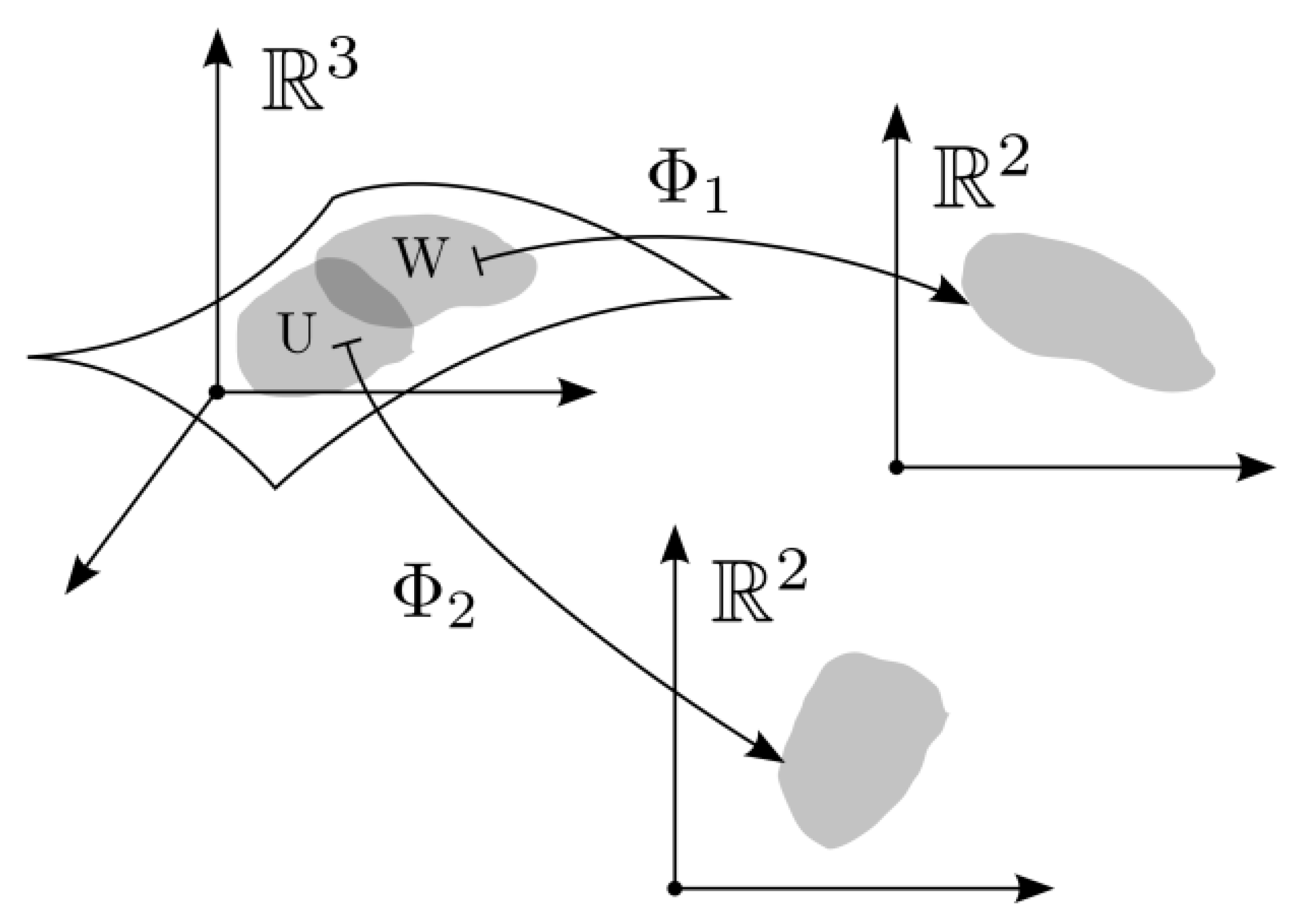
Figure 5.
Histogram of density values ρ(xi) across the dataset. Published with MATLAB® R2025b 11.
Figure 5.
Histogram of density values ρ(xi) across the dataset. Published with MATLAB® R2025b 11.
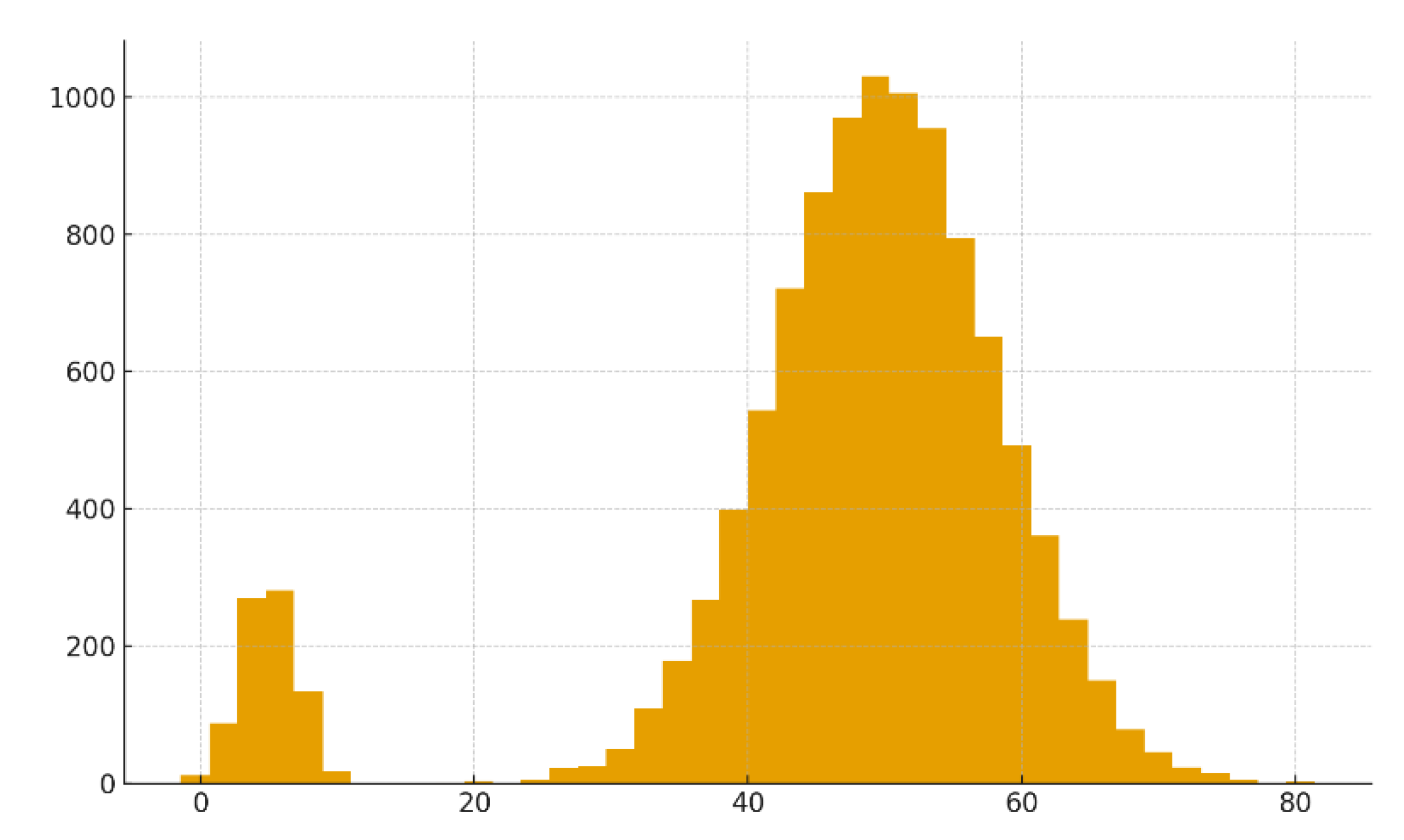
Figure 6.
Distribution of Euclidean distances among five-dimensional behavioral vectors. Published with MATLAB® R2025b 12.
Figure 6.
Distribution of Euclidean distances among five-dimensional behavioral vectors. Published with MATLAB® R2025b 12.
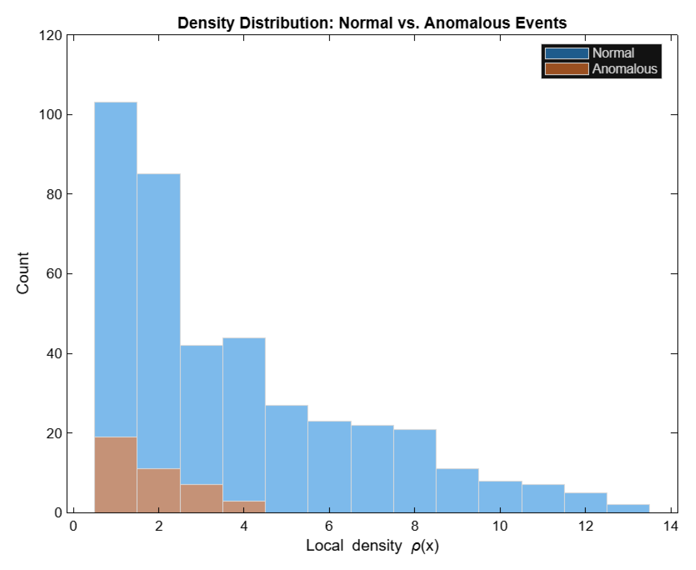
Table 1.
Dataset and preprocessing summary.
| Step | Description |
|---|---|
| Dataset | Kyoto 2006+ 5(December 2015 full month, ~7.9M flows) |
| Sampling strategy | Uniform random sampling across all 31 days |
| Sample size | 10,000 behavioral events |
| Dimensionality | 5 behavioral dimensions (normalized) |
| Normalization | Z-score applied to each dimension |
| Distance metric | Euclidean distance in R5 |
| Radius estimation | Median 20-NN distance: 0.084 |
| Density threshold | MinPts=50 |
Table 2.
Overview of the density–metric manifold pipeline used for anomaly separation. Behavioral events are embedded in R5, endowed with the Euclidean metric, and evaluated by the ε-neighborhood density operator . The manifold is partitioned into the normal region and the anomalous region according to the density threshold MinPts.
| Raw behavioral events | Embedding in R5 | Metric structure | Density operator | Manifold partition & anomaly decision |
|---|---|---|---|---|
| (System Calls, flows, alerts, …) |
Step 1 – Behavioral embedding xi = (d1,i, d2,i, d3,i, d4,i, d5,i) ∈ ℝ5 |
Step 2 – Metric structure on M⊂ℝ5 | Step 3 – Density operator | Normal region |
| dimension 1: Event Frequency dimension 2: Entropy dimension 3: Inter–arrival Variance dimension 4: Unique Endpoints dimension 5: z – Score Deviation |
metric balls Bε(x) | Mnorm = { x : ρ (x) ≥ MinPts } connected high–density core |
||
| Nε(xi) = { xj ∈ M : d(xi, xj) ≤ ε} ρ (xi) = |Nε(xi)| ε chosen as median 20-NN distance |
Anomalous region | |||
| Manom = { x : ρ (x) < MinPts } isolated low–density components | ||||
| Anomaly labels / security alerts | ||||
Table 4.
Density statistics for the two regions of the manifold.
| Statistic | Normal Points | Anomalous Points |
|---|---|---|
| Number of points | 7059 | 2941 |
| Mean density | 830 | 14 |
| Minimum density | 50 | 1 |
| Maximum density | 2302 | 48 |
| 1st percentile | 55 | 1 |
| 25th percentile | 171 | 2 |
| 50th percentile (median) | 265 | 10 |
| 75th percentile | 600+ | 22 |
| 99th percentile | > 1500 | 48 |
Table 6.
Variance explained by the first PCA components.
| Component | Variance Explained |
|---|---|
| PC1 | 28% |
| PC2 | 16% |
| PC3 | 13% |
| PC4 | 10% |
| PC5 | 8% |
Disclaimer/Publisher’s Note: The statements, opinions and data contained in all publications are solely those of the individual author(s) and contributor(s) and not of MDPI and/or the editor(s). MDPI and/or the editor(s) disclaim responsibility for any injury to people or property resulting from any ideas, methods, instructions or products referred to in the content. |
© 2025 by the authors. Licensee MDPI, Basel, Switzerland. This article is an open access article distributed under the terms and conditions of the Creative Commons Attribution (CC BY) license (http://creativecommons.org/licenses/by/4.0/).
Copyright: This open access article is published under a Creative Commons CC BY 4.0 license, which permit the free download, distribution, and reuse, provided that the author and preprint are cited in any reuse.


