
Submitted:
27 October 2025
Posted:
28 October 2025
You are already at the latest version
Abstract
Anomalies in real systems differ widely in impact, as such, missing a high-severity event can be far costlier and consequential than flagging a benign outlier. This paper introduces Severity-Regularized Deep Support Vector Data Description, an extention of deep support vector data description that incorporates severity for various anomaly types, reflecting the application-specific importance assigned to each type. The formulation retains the well-known deep support vector data description decision geometry and scoring system while allowing for specific control over the balance between false alarm rate and the prioritization of detecting anomalies with greater impact. In the proposed loss function, we introduce regularizing parameters that control the importance assign to each anomaly type. Experiments are carried out on a demanding simulated dataset and a real-world intrusion detection case study utilizing the Australian Defence Force Academy Linux Dataset. The results demonstrate the effectiveness of the proposed approach in detecting highly severe anomalies while maintaining competitive overall performance.
Keywords:
anomaly detection
; cybersecurity
; Deep SVDD
; host-based intrusion detection (HIDS)
; severity-aware intrusion detection
; Severity-Regularized Deep SVDD (SR-DeepSVDD)
; Support Vector Data Description (SVDD)
MSC: 68T07; 68T10
1. Introduction
Anomaly detection is a machine learning technique that has been widely applied in many domains, including cybersecurity, finance, healthcare, the industrial internet of things, and disaster management [1,2,3,4,5]. The objective of anomaly detection methods is to detect anomalous behavior by capturing a proper representation of normal operating conditions. However, anomalies are often heterogeneous in terms of their severity and consequences, where some have a low impact, while others are high-severity events that expose safety, privacy, or system availability. Failing to detect high-severity anomalies can lead to catastrophic damage.
Various deep learning methods have been developed for anomaly detection that utilize normal observation labels in training the method. A deep variant of support vector data description (SVDD) was developed by Ruff et al. [6]. To improve one-class separation, deep autoencoding of SVDD was proposed [7]. To preserve local data, structured deep structure preservation SVDD was developed [8]. Variational autoencoder (VAE)-based deep support vector data description (DeepSVDD) has been introduced to shape the latent space before applying the SVDD objective for effective feature representation [9]. Contrastive DeepSVDD was developed to enhance the feature representation from large data sets [10]. To utilize labeled anomaly information in combination with labeled normal in DeepSVDD, Deep semi-supervised anomaly detection (DeepSAD) was proposed [11]. While effective, these methods do not incorporate anomaly labels in their loss function or implicitly assume that all anomalies have the same level of severity and impact. As such, an approach that assigns a higher priority to severe anomaly detection can enhance critical anomaly detection.
In practice, several deep learning-based anomaly detection methods have been applied to cybersecurity. In aviation, a VAE-based DeepSVDD model on automatic dependent surveillance-broadcast (ADS-B) has been applied to detect communication tampering and anomalies [12]. Temporal convolutional networks and transformer-based SVDD were used to detect anomalies in ADS-B generated by denial of service (DoS) attacks [13]. In vehicular networks, intrusion detection systems (IDS), a collaborative DeepSVDD method of multiple agents, were proposed to improve vehicular network protection by reducing false negative rates [14]. A convolutional autoencoder combined with SVDD was introduced for IDS to improve the performance of industrial control systems (ICS) [15]. A lightweight network intrusion detection system for industrial IoT based on incremental SVDD was introduced to improve detection accuracy [16]. In smart electric grids, DeepSVDD has been applied to detect false data injection [17]. An adaptive policy-based anomaly control for cybersecurity has been introduced to reduce distributed DoS attacks that uses an out-of-distribution detector for neural networks combined with DeepSVDD [18]. A deep one-class support vector machine coupled with an autoencoder has been applied to IDS to predict deviations from normal network behavior at inference [19]. Despite improved intrusion detection performance, these methods assume that all types of attacks and anomalies have the same levels of impact and severity, while rarely using their labels in training. As such, assigning the same detection priority to all anomaly types, whereas in real-world applications, the anomalies vary based on their impact and severity. In cybersecurity risk management, for example, undetected attacks that create unauthorized (super)user accounts enable persistent footholds and escalation that would amplify damage, increase data loss and breach risk, complicate containment and raise recovery costs [20]. Therefore, an intrusion detection model that can prioritize the detection of more severe and impactful cyberattacks is essential for effective cybersecurity management.
Motivated by these challenges, this paper presents Severity-Regularized Deep SVDD (SR-DeepSVDD). Specifically, we propose a novel DeepSVDD variant that incorporates anomaly severity across multiple anomaly types based on application-specific importance assigned to each type. In the proposed loss function, we introduce regularizing parameters that control the importance assigned to each anomaly type. To our knowledge, we develop the first application of SR-DeepSVDD for intrusion detection in cybersecurity to improve detection rates of highly severe anomalies using the Australian Defence Force Academy Linux Dataset (ADFA-LD). Experiments are carried out on a simulated dataset and a real-world intrusion detection case study to demonstrate SR-DeepSVDD’s effectiveness in detecting highly severe anomalies while maintaining competitive overall performance.
The remainder of the paper is organized as follows. Section 2 proposes the newly developed SR-DeepSVDD method. Section 3 presents our experiments on the simulation dataset. An Intrusion Detection System based on SR-DeepSVDD is introduced in the case study in Section 4. Section 5 draws conclusions and future work directions.
2. Severity-Regularized Deep Support Vector Data Description
In this section, we develop a severity-aware extension of Deep SVDD. The primary concept is to maintain the Deep SVDD decision boundary within a deep latent space while incorporating anomaly-type severity regularization into the training objective. We first establish the notation, then briefly recap Deep SVDD and its limitations, and finally introduce a severity-regularized objective and an optimization procedure to obtain an effective decision boundary.
We consider anomaly detection with labeled normal observations and labeled anomaly observations partitioned into K anomaly types. Let denote the N normal training observations, where . For each type of anomaly , let denote the labeled anomalies of that type. A deep encoder maps the inputs into a latent space, producing embeddings , in which we learn a hypersphere of normality with center and radius .
2.1. Introduction to Deep SVDD
The goal of Deep SVDD is to learn a hypersphere representation from normal observation embeddings centered around a fixed latent point such that proximity to that center indicates normality [6]. In the fixed center (one-class) formulation, the encoder parameters are learned by minimizing the average squared distance of normal embeddings to the center with weight decay.
where is the layerwise weight-decay coefficient.
A soft-boundary approach concurrently learns a nonnegative radius and penalizes only the normals that lie outside the sphere. The parameter governs the permissible fraction of violations.
In practice, the center is initialized from a warm-up pass on normals (e.g., the mean of initial embeddings) and then fixed to stabilize optimization, and bias terms are removed from the network to prevent degenerate collapse [6].
Although effective as a one-class learner, the original formulation does not incorporate labeled anomalies or distinguish among anomaly types with different operational consequences. As such, highly severe anomalies can be overlooked and treated as normal in the monitoring phase. This limitation drives the development of a severity-aware extension that structures the latent space and boundary to preferentially identify higher-severity anomaly types.
2.2. Severity-Regularized Deep SVDD
In order to distinguish between anomaly types while preserving the SVDD geometry, we propose a new soft-boundary Deep SVDD objective with type-specific severity-regularized push-out penalties.
where is the same soft-boundary parameter as in (2); encodes the importance of the anomaly type k, and is an optional clearance margin for that type.
In the proposed formulation, the term discourages an unnecessarily large hypersphere, while the hinge in the second term activates only for normal embeddings that fall outside the boundary; thus, those outlying normals are pulled inward. The parameter controls how tight the sphere is allowed to be by setting the tolerated fraction of such violations, a smaller yields a tighter hypersphere (fewer allowed outliers), and a larger permits more normal observations outside the hypersphere, obtaining a wider boundary. Normalization by N keeps the contribution per normal observation roughly scale-free as the training dataset grows larger. The third term adds the severity-regularized anomaly push-out per anomaly type. The hinge activates only when an anomaly of type k is inside the sphere or within the type-specific margin of width . When active, it pushes those embeddings outward, either increasing their distance from in the latent space or, through the joint optimization, discouraging an increase of R that would otherwise encapsulate them. The weight scales the importance of anomaly type k where a larger pushes type k anomalies out of the hypersphere, and the margin allows for an increased gap between type k anomalies and the boundary. Dividing by balances the per-type influence so that abundant or rare anomaly types do not dominate simply due to sample count. The last term is a layerwise weight decay that regularizes the network parameters . Crucially, these additions do not alter the decision geometry, and the score persists as . This formulation enhances the representation and the hypersphere to facilitate stronger separation for more severe anomaly types.
If all severity weights are set to zero, i.e., for every , the push-out term is eliminated and reduces to
which is exactly the soft-boundary Deep SVDD objective in (2). Thus, Deep SVDD is recovered as a special case of the proposed formulation.
Alternatively, setting produces a center-fixed SR-DeepSVDD with score and anomaly push-out . Its objective is
For smoother magnitude-aware gradients, one may square the hinge terms in (3) (and (4)). Specifically, replace and by their squared forms
This preserves zero loss for non-violations and leaves the decision score unchanged, while imposing a quadratic penalty on margin violations that makes the (L2-loss) objective differentiable and yields gradients that scale linearly with the violation—properties known to simplify and stabilize optimization [21,22,23]; see also the motivation for smoothing non-smooth hinge losses to
For a test point , we score anomalies by the signed squared radial distance from its embedding to the center. Let and denote the trained network parameters and radius; then
According to this scoring convention, points located outside the hypersphere (anomalies) have , inliers (normals) have , and boundary points correspond to . In the center-fixed variant (), this reduces to the unsigned distance . In addition, training data are not required at the prediction time. The model is entirely defined by , the fixed , and the in the soft-boundary variant, which facilitates low-memory and rapid inference by a single forward pass through .
Alternatively, an inference mechanism can be defined post-training and during validation. Given scores , a threshold can be selected using a held-out validation set where common choices could be to fix a target false-alarm rate on validation normals and set to the corresponding quantile, or maximizing a utility that reflects type importance, e.g., . This post-training calibration does not alter the learned representation or decision geometry.
2.3. Optimization of Severity-Regularized Deep SVDD
The network parameters are optimized by stochastic gradient methods such as stochastic gradient descent (SGD), Adam, and AdamW on the squared-hinge SR-DeepSVDD objective in (5), using backpropagation and standard mini-batch training. This training procedure is in line with the deep SVDD training practices and scales linearly with the number of batches [6,24,25]. We first run a short warm-up on normal data to initialize the center as the mean embedding and then keep fixed. To avoid trivial “hypersphere collapse,” we use bias-free layers as suggested for Deep SVDD [6]. Rather than backpropagating through the radius, we adopt a lightweight alternating update: within each epoch, R is held fixed while is updated; after the epoch, we refresh R by setting to the empirical -quantile of the squared distances of training normals, consistent with the soft-boundary -property (roughly of normals may lie on or outside the sphere) [6,26]. Mini-batches may include both normals and any labeled anomalies; the anomaly push-out term is applied per type with weights , margins , and normalization by . This epoch-wise quantile step is a fast block-coordinate update for R that empirically tracks the line-search update advocated in the original Deep SVDD when using the plain hinge [6]. In our implementation, we use the squared hinge in (5) for smoother, magnitude-aware gradients while leaving the decision score unchanged.
2.4. Calibration of Severity Weights and Margins
The severity weights , importance of anomaly type k, and margins , desired clearance for type k are tuned on held-out validation set to prioritize the detection of more consequential and severe anomaly types while controlling false alarms
where is the detection rate for type k at threshold and is a target false alarm rate (FAR) on validation normals.
A practical approach is to maximize an application utility, for example, a weighted sum of per anomaly type detection rates, subject to a target false-alarm rate on validation normals. In choosing search spaces, can be explored on a logarithmic grid and on a compact grid in latent-distance units with application-dependent bounds. Performance is typically most sensitive near small magnitudes and exhibits diminishing returns as values grow. While holding the other hyperparameters fixed, the type-k detection rate generally increases monotonically with and until saturation. Increasing multiple simultaneously can reduce the distinction between types of anomalies and should reflect the true severity or operational cost.
The soft-boundary parameter also shapes calibration. A larger tightens the boundary (smaller R) and could increase detection at the cost of higher false alarms. In contrast, a smaller widens the boundary (larger R), reducing false alarms but potentially lowering detection unless and/or are increased.
In calibration procedures, it is essential to consider class imbalance to ensure that infrequent but critical types are not dominated by more common ones, which can be achieved through per anomaly type application-based utility or normalization. Selections should aim for operating points where further increases in or result in small marginal gains in detection. Throughout, these choices preserve the standard SVDD decision score and its interpretation.
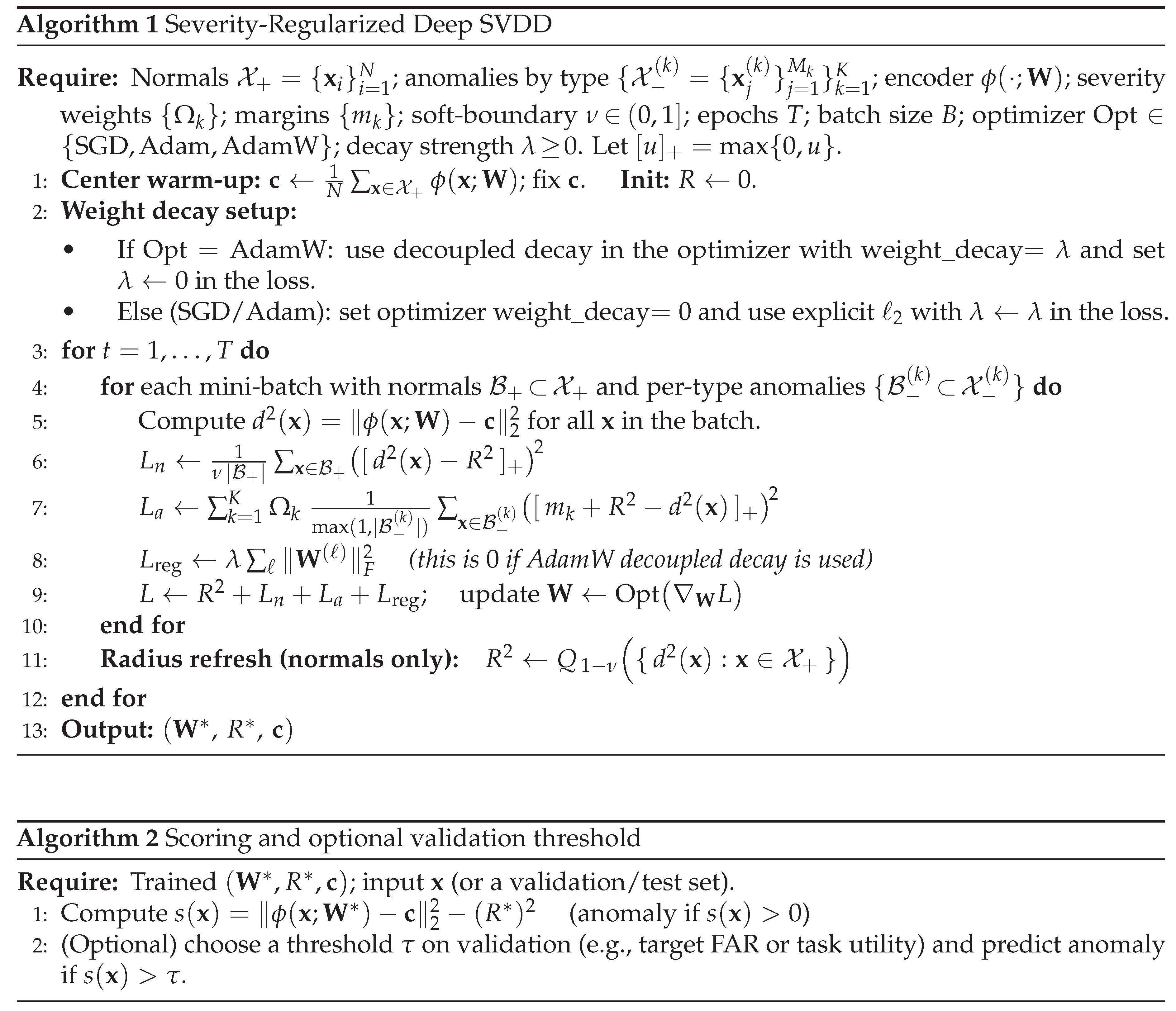
Algorithm 1 summarizes SR-DeepSVDD training while Algorithm 2 describes inference via scoring and optional validation-time threshold calibration.
3. Experiments on Simulated Data
In this section, we evaluate the proposed Severity-Regularized Deep SVDD (SR-DeepSVDD) against three baseline methods: Deep SVDD [6], one class suport vetor machines (OC-SVM) [27], and classical SVDD with an RBF kernel (SVDD-RBF)[26]. We also compare it to an ablation of SR-DeepSVDD (SR-DeepSVDD-NS) where we do not distinguish between anomaly types, which can be considered a variant of DeepSAD without unlabeled data [11]. The study uses a two-dimensional simulated dataset that induces an irregular normal region (banana shape) and two anomaly types with different severities.
3.1. Experimental Setup
We generate a total of observations in : 700 normals and anomalies across two types. Normal samples with a mean vector are sampled from banana-shaped data. We define severe anomalies as Type-1, drawn from with and diagonal covariance (off-diagonal entries are zero). Non-severe anomalies are defined as Type-2, sampled from with and diagonal covariance (off-diagonal entries are zero). Data are split into train, validation, and test sets with stratified ratios over the normal class and each anomaly type. A representative training split is shown in Figure 1.
For evaluation, we report per–anomaly-type recall, precision, and F1 using the anomaly-type index . For each k, we compute the confusion counts on the subset . The typewise metrics are
In addition, we report the FAR on normals,
where and are computed over all normal samples. Here, , , , and .
We compare SR-DeepSVDD against Deep SVDD, OC-SVM, and SVDD-RBF methods. All deep methods share the same encoder capacity for fairness—a bias-free multi-layer perceptron (MLP) with two hidden layers (64, 32) and a 16-dimensional embedding—and are trained with AdamW for 50 epochs using mini-batches of size 128. For SR-DeepSVDD we use the soft-boundary objective with squared hinges and , severity weights and margins are set to and , and optimization uses AdamW (learning rate with weight decay ). At validation, the threshold is chosen to maximize the Type-1 detection rate subject to a false alarm cap on validation normals. Deep SVDD uses the same encoder and with a squared hinge loss, trained on labeled normals only with AdamW (learning rate , weight decay ); its is selected on validation to maximize F1 under the same FAR cap. OC-SVM employs an RBF kernel with and , and makes decisions by its native decision boundary. SVDD-RBF uses with and also makes decisions using its native decision boundary. Moreover, to evaluate the effectiveness of severity weights and margins, we report an ablation, SR-DeepSVDDNS, which is identical to SR-DeepSVDD in terms of architecture, optimization, and validation policy but sets anomaly-specific parameters and , thereby does not differentiate between anomaly types.
To assess robustness, we repeat the entire procedure over 10 random seeds. For all methods, we select—per seed—the configuration according to the validation policy of each method described above. We report the Type-1 score as mean ± standard deviation (SD) across seeds. We also show the performance over a single selected seed for all performance metrics.
3.2. Results and Analysis
Table 1 lists the overall and per–anomaly-type metrics (including FAR) on a representative seed, while Table 2 summarizes the overall F1 across the 10 seeds as mean ± SD. The decision boundaries for each method are visualized in Figure 2, where the heat map shows the anomaly score and the dashed curve denotes the selected threshold .Table 1 lists the overall and per–anomaly-type metrics (including FAR) on a representative seed, while Table 2 summarizes the overall F1 across the 10 seeds as mean ± SD. The corresponding score fields and calibrated decision boundaries for each method are visualized in Figure 2, where the heat map shows the anomaly score and the dashed curve denotes the selected threshold .
The OC-SVM algorithm establishes a wide, radially shaped boundary (Figure 2 a) that identifies numerous anomalies but also inaccurately categorizes peripheral normals as anomalies, aligning with the elevated False Alarm Rate (FAR) detailed in Table 1.SVDD-RBF adjusts its boundary to align more closely with the normal distribution density (Figure 2 b), resulting in a more balanced precision-recall trade-off compared to OC-SVM and generating fewer false alarms on normals. DeepSVDD, trained using normal observations, establishes an excessively broad decision boundary (Figure 2 c). This boundary successfully encompasses distant normal observations but also inadvertently includes Type-1 anomalies, resulting in a compromise. Consequently, this negatively impacts its typewise F1 score, despite maintaining reasonable precision, and reduces the detection rate for Type-1 anomalies. Including anomaly information into decision boundary training, although without considering anomaly type severity, SR-DeepSVDD-NS improves the deep boundary as the boundary expands more symmetrically around the normal region while trying to push anomalies out (Figure 2 d), producing solid, uniform gains across types but without explicitly prioritizing the severe class.
In contrast, SR-DeepSVDD contracts the decision boundary to be more precise, especially in areas where severe Type-1 anomalies are concentrated (Figure 2 e). This method effectively isolates the top cluster of severe anomalies better than the ablation (SR-DeepSVDD-NS) approach, as shown by the improved detection rate for the Type-1 anomaly, while still providing strong detection rates for lower-priority anomaly types. This underscores the importance of the newly introduced severity importance weights, which emphasize the detection of severe anomalies. Moreover, the seed-level results in Table 2 further indicate that SR-DeepSVDD is consistently the most robust across random initializations, with SR-DeepSVDD-NS following behind.
3.3. Effect of Severity Importance Weight on Performance
We study how the severity weight placed on Type-1 anomalies () affects SR-DeepSVDD while keeping all other settings fixed. Figure 3 plots the Type-1 detection rate () on the left y-axis colored with a blue line and the overall F1 score on the right y-axis colored with a red against on the x-axis. When is very small, the loss under-weights Type-1 violations and the model behaves similarly to a non-distnguishing variant, producing weak and only moderate F1. As increases to a moderate range, both and F1 improve sharply and remain high over a wide range, indicating that giving meaningful preference to the severe class helps the network push Type-1 anomalies farther beyond the boundary while maintaining overall balance. Pushing to very large values eventually degrades both curves, as excessive emphasis on the severe class distorts the boundary, trading off precision and harming overall F1. These results suggest careful selection of is required over the validation set where moderate values deliver a favorable trade-off between prioritizing detection of type k anomalies and preserving overall performance.
4. Case Study: Severity-Regularized Deep SVDD for Intrusion Detection in Cybersecurity
This section presents our case study on host-based intrusion detection. We analyzed Linux system-call sessions from the Australian Defence Force Academy Linux Dataset (ADFA-LD) [28,29]. It captures normal activity and multiple attack families under controlled conditions. The data set has family-level labels for both attack and normal sessions.
4.1. Intrusion Detection Experiment Setup
To reflect operational priorities in cybersecurity risk management, we introduce a severity importance mechanism over attack families. According to a report prepared by the National Institute of Standards and Technology, undetected intrusions that create unauthorized (super)user accounts allow for persistent presence and escalation, potentially exacerbating harm, enhancing data loss and breach risk, complicating containment efforts, and increasing recovery expenses. [20]. Therefore, the "Adduser" attack family that resembles this type of threat in ADFA-LD has been considered as the severe anomaly type (Type-1 anomalies) in our case study experiments. In contrast, the rest of the families have been considered as non-severe (Type-2 anomalies) for the purpose of this experiment. Thus, the objective is to be able to detect "Adduser" intrusions with higher accuracy without sacrificing the overall performance of the intrusion detection model.
We represent each session as a fixed-length vector. Traces are tokenized, and term frequency–inverse document frequency (TF–IDF) is computed over n-gram lengths 1–4 with sublinear TF. The TF–IDF model is fit once on all training sessions, including normal and anomaly traces. To reduce out-of-vocabulary drift, the fitted transform is applied unchanged to validation and testing sessions. In parallel, we compute the length of the session, the logarithmic length, the number of unique tokens, the Shannon entropies of the unigram/bigram Shannon, the proportion of the most frequent token and the cumulative proportion of the three most frequent tokens, the Gini unigram coefficient, burstiness (count coefficient of variation in non-overlapping windows of 50), and an n-gram diversity ratio. These features are standardized using means and standard deviations from training normals only. Finally, TF–IDF is densified and concatenated with the standardized tabular block to produce a single input vector per session. This follows common intrusion detection systems practice while ensuring reproducibility and compatibility with deep boundary learners that require fixed-dimensional inputs [30,31,32,33].
The dataset is partitioned at the session level where normals arae randomly partitioned as , and into training, validation, and test sets, respectively, while anomalies are split, per attack family, with ,, and into training, validation, and testing sets. Training of the baseline methods uses the training normals only, while SR-DeepSVDD training uses the same training normals together with labeled anomalies. All deep models share the same MLP encoder (two hidden layers of sizes 512 and 256 with a 64-dimensional latent representation). All methods use for training.
All methods use the same operating-point calibration policy as in our simulated study. SR-DeepSVDD and its no-severity ablation, SR-DeepSVDD-NS, share the training setup with AdamW optimizer (learning rate , refresh rate 50 epochs, batch size 128, weight decay ). They differ only in severity settings, where SR-DeepSVDD uses with margins , whereas SR-DeepSVDD-NS sets . DeepSVDD uses AdamW optimizer (learning rate , refresh rate 10 epochs, batch size 128, and weight decay ). OC-SVM is trained with and SVDD-RBF with .
4.2. Intrusion Detection Results and Analysis
Table 3 summarizes the overall and typewise performance on ADFA-LD where Type-1 denotes the highest severity targeted anomaly (Adduser attack family) and Type-2 denotes the lowest severity attack sessions. OC-SVM shows poor performance in terms of F1 and detection rate for the severe attack session, while also underperforming in capturing normal sessions successfully due to the increased FAR. SVDD-RBF shows better performance in detecting the severe attack sessions, as it builds a narrower decision boundary; however, this causes an increase in normal sessions being detected as attacks, thereby increasing its FAR.
Since DeepSVDD does not include an anomaly push-out term in its loss function, it produces a conservative operating point that broadens the decision boundary to capture normal sessions effectively but sacrifices recall (detection rate) on both types of anomalies, thereby reducing its typewise F1 despite reasonable precision.
Incorporating attack sessions into boundary learning (without severity weighting), the ablation, SR-DeepSVDD-NS, constructs a tighter boundary around normal sessions compared to DeepSVDD, pushing attack sessions outward, producing enhanced uniform gains across attack session types at a low FAR, yet without explicitly prioritizing the adduser attack family.
Meanwhile, the severity-aware SR-DeepSVDD contracts and sharpens the decision boundary where the severe attack sessions are concentrated, isolating these instances more effectively than the ablation, while maintaining strong performance on lower-priority attack families and keeping FAR competitively low. The improvements align with the severity importance weights that prioritize the detection of severe attack sessions. These results indicate the added advantages of using SR-DeepSVDD in cybersecurity risk management, specifically intrusion detection.
5. Conclusions
This paper presents Severity-Regularized Deep SVDD, a principled extension of Deep SVDD that incorporates anomaly-type severity into the training objective. This is achieved by introducing anomaly type-specific push-out penalties, which have adjustable importance weights and margins. The formulation retains the well-known SVDD decision geometry and scoring system while allowing for specific control over the balance between FAR and the prioritization of detecting anomalies with greater impact. In both a demanding simulated environment and a host-based intrusion detection cybersecurity case study utilizing ADFA-LD, SR-DeepSVDD consistently achieved the most robust overall performance compared to other one-class and deep baseline algorithms. Crucially, the approach enhanced the detection of the targeted (severe) anomaly type without increasing false positive rates on normal instances, while maintaining superior performance on lower-priority anomaly types. The ablation study without severity weights, SR-DeepSVDD-NS, validated the benefit of integrating labeled anomalies into boundary learning.
From an operational perspective, SR-DeepSVDD provides practitioners with a distinct severity control: the importance weights () and margins () can be adjusted using validation data to prioritize domain-critical attacks, such as account-creation intrusions, while ensuring that the overall FAR remains within acceptable limits. This approach does not introduce additional overhead inference time beyond the standard forward pass and threshold comparison, making it suitable for real-time monitoring.
SR-DeepSVDD utilizes labeled anomaly types to guide severity-aware training. In domains with scarce labels, semi-supervised approaches for uncovering and assigning importance to latent anomaly clusters represent a promising future research direction. Future work could include learning and based on task-level utilities or costs, and the implementation of dynamic or data-dependent reweighting that adapts to drift during online monitoring. Collectively, these advancements can further enhance severity-based anomaly detection in applications where safety and security are critical.
Data Availability Statement
The code for SR-DeepSVDD implementation is available at https://github.com/ alhinditaha/SR-DeepSVDD.
Acknowledgments
The project was funded by KAU Endowment (WAQF) at King Abdulaziz University, Jeddah, Saudi Arabia. The authors, therefore, acknowledge with thanks WAQF and the Deanship of Scientific Research (DSR) for technical and financial support.
Conflicts of Interest
The authors declare no conflicts of interest
Abbreviations
The following abbreviations are used in this manuscript:
| Adam | Adaptive Moment Estimation |
| AdamW | Adaptive Moment Estimation with (decoupled) Weight decay |
| DeepSVDD | Deep Support Vector Data Description |
| IDS | Intusion Detection System |
| OC-SVM | One-Class Support Vector Machine |
| RBF | Radial Basis Function |
| SVDD | Support Vector Data Description |
| TF–IDF | Term Frequency–Inverse Document Frequency |
References
- Chatterjee, A.; Ahmed, B.S. IoT anomaly detection methods and applications: a survey. Internet of Things 2022, 19, 100568, doi:. [CrossRef]
- Alhindi, T.J.; Alturkistani, O.; Baek, J.; Jeong, M.K. Multi-class support vector data description with dynamic time warping kernel for monitoring fires in diverse non-fire environments. IEEE Sensors Journal 2025, doi:10.1109/JSEN.2025.3561725.
- Nassif, A.B.; Talib, M.A.; Nasir, Q.; Dakalbab, F.M. Machine learning for anomaly detection: A systematic review. IEEE Access 2021, 9, 78658–78700, doi:10.1109/ACCESS.2021.3083060.
- Bakumenko, A.; Elragal, A. Detecting anomalies in financial data using machine learning algorithms. Systems 2022, 10, 130, doi:. [CrossRef]
- Samariya, D.; Ma, J.; Aryal, S.; Zhao, X. Detection and explanation of anomalies in healthcare data. Health Information Science and Systems 2023, 11, 20, doi:. [CrossRef]
- Ruff, L.; Vandermeulen, R.; Goernitz, N.; Deecke, L.; Siddiqui, S.A.; Binder, A.; Müller, E.; Kloft, M. Deep one-class classification. In Proceedings of the International Conference on Machine Learning 2018; pp. 4393–4402.
- Hojjati, H.; Armanfard, N. DASVDD: Deep autoencoding support vector data descriptor for anomaly detection. IEEE Transactions on Knowledge & Data Engineering 2024, 36, 3739–3750, doi:10.1109/tkde.2023.3328882.
- Zhang, Z.; Deng, X. Anomaly detection using improved deep SVDD model with data structure preservation. Pattern Recognition Letters 2021, 148, 1–6, doi:. [CrossRef]
- Zhou, Y.; Liang, X.; Zhang, W.; Zhang, L.; Song, X. VAE-based Deep SVDD for anomaly detection. Neurocomputing 2021, 453, 131–140, doi:. [CrossRef]
- Xing, H.-J.; Zhang, P.-P. Contrastive deep support vector data description. Pattern Recognition 2023, 143, 109820, doi:. [CrossRef]
- Ruff, L.; Vandermeulen, R.A.; Görnitz, N.; Binder, A.; Müller, E.; Müller, K.-R.; Kloft, M. Deep semi-supervised anomaly detection. In Proceedings of the International Conference on Learning Representations 2020.
- Luo, P.; Wang, B.; Li, T.; Tian, J. ADS-B anomaly data detection model based on VAE-SVDD. Computers & Security 2021, 104, 102213, doi:. [CrossRef]
- Luo, P.; Wang, B.; Tian, J. TTSAD: TCN-Transformer-SVDD model for anomaly detection in air traffic ADS-B data. Computers & Security 2024, 141, 103840, doi:. [CrossRef]
- Mai, J.; Wu, Y.; Liu, Z.; Guo, J.; Ying, Z.; Chen, X.; Cui, S. Anomaly detection method for vehicular network based on collaborative deep support vector data description. Physical Communication 2023, 56, 101940, doi:. [CrossRef]
- Wang, J.; Li, P.; Kong, W.; An, R. Unknown security attack detection of industrial control system by deep learning. Mathematics 2022, 10, 2872, doi:. [CrossRef]
- Gyamfi, E.; Jurcut, A.D. Novel online network intrusion detection system for industrial IoT based on OI-SVDD and AS-ELM. IEEE Internet of Things Journal 2022, 10, 3827–3839, doi:10.1109/JIOT.2022.3172393.
- Habbak, H.; Mahmoud, M.; Fouda, M.M.; Alsabaan, M.; Mattar, A.; Salama, G.I.; Metwally, K. Efficient one-class false data detector based on deep svdd for smart grids. Energies 2023, 16, 7069, doi:. [CrossRef]
- Sakong, W.; Kim, W. An adaptive policy-based anomaly object control system for enhanced cybersecurity. IEEE Access 2024, 12, 55281–55291, doi:10.1109/ACCESS.2024.3389067.
- Bountzis, P.; Kavallieros, D.; Tsikrika, T.; Vrochidis, S.; Kompatsiaris, I. A deep one-class classifier for network anomaly detection using autoencoders and one-class support vector machines. Frontiers in Computer Science 2025, Volume 7 – 2025, doi:10.3389/fcomp.2025.1646679.
- Nelson, A.; Rekhi, S.; Souppaya, M.; Scarfone, K. Incident Response Recommendations and Considerations for Cybersecurity Risk Management; 2025.
- Hsieh, C.-J.; Chang, K.-W.; Lin, C.-J.; Keerthi, S.S.; Sundararajan, S. A dual coordinate descent method for large-scale linear SVM. In Proceedings of the 25th International Conference on Machine Learning (ICML ’08) 2008; pp. 408–415, doi:. [CrossRef]
- Steinwart, I. Sparseness of support vector machines. Journal of Machine Learning Research 2003, 4, 1071–1105.
- Fan, R.-E.; Chang, K.-W.; Hsieh, C.-J.; Wang, X.-R.; Lin, C.-J. LIBLINEAR: A library for large linear classification. Journal of Machine Learning Research 2008, 9, 1871–1874.
- Kingma, D.P.; Ba, J. Adam: A Method for Stochastic Optimization. In Proceedings of the International Conference on Learning Representations 2015.
- Loshchilov, I.; Hutter, F. Decoupled Weight Decay Regularization. In Proceedings of the International Conference on Learning Representations 2019.
- Tax, D.M.J.; Duin, R.P.W. Support Vector Data Description. Machine Learning 2004, 54, 45–66.
- Manevitz, L. M.; Yousef, M. One-class SVMs for document classification. Journal of Machine Learning Research 2001, 2, 139–154.
- UNSW Canberra. ADFA IDS (Intrusion detection systems) datasets comprising labeled host, network and windows stealthy attacks settings. Harvard Dataverse 2024, V1, doi:. [CrossRef]
- Creech, G.; Hu, J. A Semantic Approach to Host-Based Intrusion Detection Systems Using Contiguous and Discontiguous System Call Patterns. IEEE Transactions on Computers 2014, 63, 807–819, doi:. [CrossRef]
- Han, X.; Cui, S.; Liu, S.; Zhang, C.; Jiang, B.; Lu, Z. Network intrusion detection based on n-gram frequency and time-aware transformer. Computers & Security 2023, 128, 103171, doi:. [CrossRef]
- Song, J.; Qin, G.; Liang, Y.; Yan, J.; Sun, M. SIDiLDNG: A similarity-based intrusion detection system using improved Levenshtein Distance and N-gram for CAN. Computers & Security 2024, 142, 103847, doi:. [CrossRef]
- Stabili, D.; Ferretti, L.; Andreolini, M.; Marchetti, M. Daga: Detecting attacks to in-vehicle networks via n-gram analysis. IEEE Transactions on Vehicular Technology 2022, 71 (11), 11540–11554.
- Sworna, Z. T.; Mousavi, Z.; Babar, M. A. NLP methods in host-based intrusion detection systems: A systematic review and future directions. Journal of Network and Computer Applications 2023, 220, 103761.
Figure 1.
Training split for the simulated study: normals (blue), Type 1 anomalies (orange), and Type 2 anomalies (green).
Figure 1.
Training split for the simulated study: normals (blue), Type 1 anomalies (orange), and Type 2 anomalies (green).
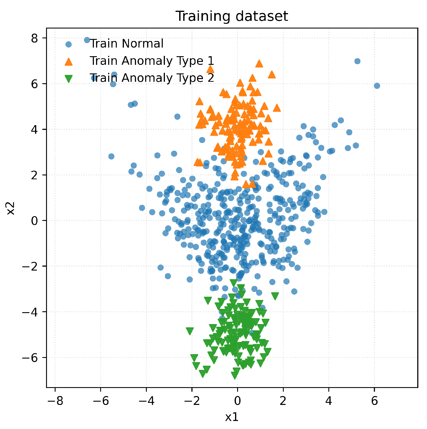
Figure 2.
Anomaly-score surfaces and decision boundaries on the simulated dataset. Heat map shows the anomaly score ; the white dashed curve is the selected decision boundary per method. Panels: (a) OC-SVM. (b) SVDD-RBF. (c) DeepSVDD. (d) SR-DeepSVDD-NS. (e) SR-DeepSVDD.
Figure 2.
Anomaly-score surfaces and decision boundaries on the simulated dataset. Heat map shows the anomaly score ; the white dashed curve is the selected decision boundary per method. Panels: (a) OC-SVM. (b) SVDD-RBF. (c) DeepSVDD. (d) SR-DeepSVDD-NS. (e) SR-DeepSVDD.
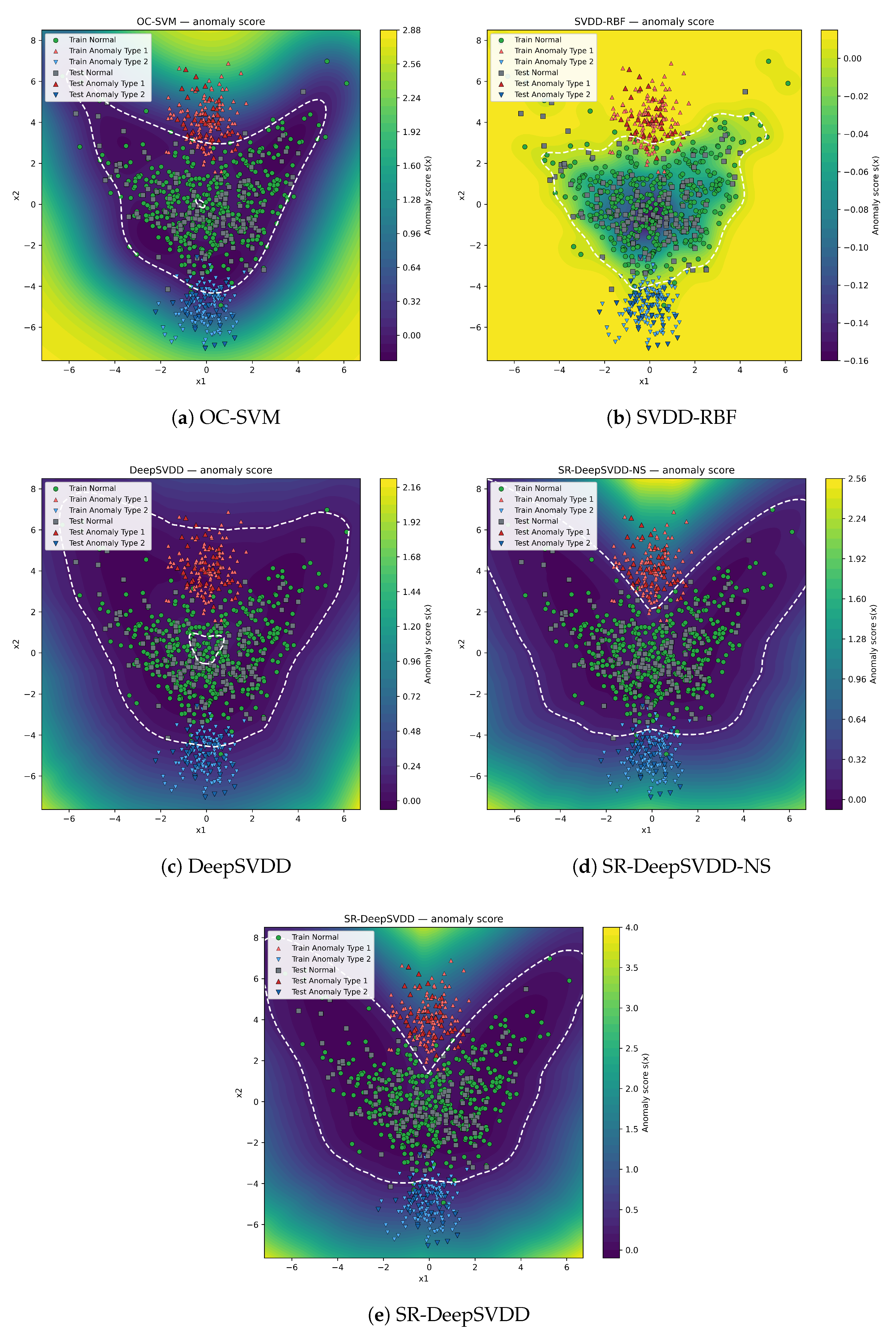
Figure 3.
Sensitivity of SR-DeepSVDD to the Type-1 severity weight . Blue: (left axis). Red: overall F1 (right axis). The x-axis lists values. Both metrics rise from small , plateau for moderate values, and deteriorate when is set too high.
Figure 3.
Sensitivity of SR-DeepSVDD to the Type-1 severity weight . Blue: (left axis). Red: overall F1 (right axis). The x-axis lists values. Both metrics rise from small , plateau for moderate values, and deteriorate when is set too high.
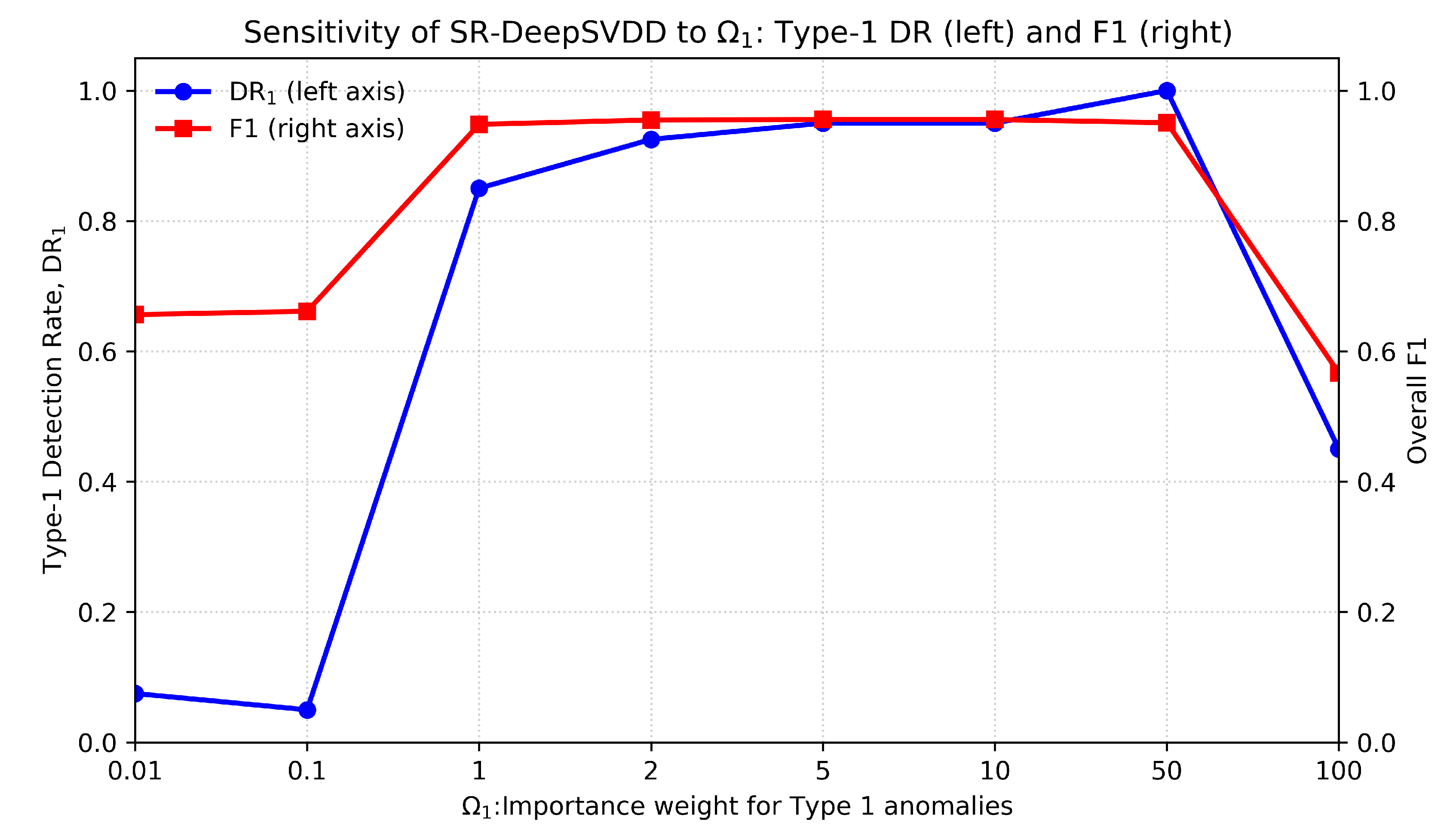

Table 1.
Overall F1, per–type precision (PREC), recall (DR), and F1, plus overall FAR on normals over an experiment on simulated data.
Table 1.
Overall F1, per–type precision (PREC), recall (DR), and F1, plus overall FAR on normals over an experiment on simulated data.
| Model | F1 (overall) | Type-1 | Type-2 | FAR | ||||
|---|---|---|---|---|---|---|---|---|
| DR1 | PREC1 | F11 | DR2 | PREC2 | F12 | |||
| OC-SVM | 0.88 | 0.88 | 0.78 | 0.82 | 0.90 | 0.78 | 0.84 | 0.07 |
| SVDD-RBF | 0.86 | 0.88 | 0.81 | 0.84 | 0.80 | 0.80 | 0.80 | 0.06 |
| DeepSVDD | 0.67 | 0.45 | 0.69 | 0.55 | 0.65 | 0.76 | 0.70 | 0.06 |
| SR-DeepSVDD-NS | 0.91 | 0.92 | 0.86 | 0.89 | 0.87 | 0.85 | 0.86 | 0.04 |
| SR-DeepSVDD | 0.95 | 0.98 | 0.89 | 0.93 | 0.95 | 0.88 | 0.92 | 0.04 |
Table 2.
F1 scores on the simulated dataset across 10 random seeds.
| Seed | OC-SVM | SVDD-RBF | DeepSVDD | SR-DeepSVDD-NS | SR-DeepSVDD |
|---|---|---|---|---|---|
| 1 | 0.78 | 0.79 | 0.31 | 0.80 | 0.93 |
| 2 | 0.75 | 0.87 | 0.40 | 0.87 | 0.89 |
| 3 | 0.81 | 0.91 | 0.46 | 0.94 | 0.94 |
| 4 | 0.80 | 0.82 | 0.39 | 0.90 | 0.93 |
| 5 | 0.88 | 0.86 | 0.67 | 0.91 | 0.95 |
| 6 | 0.80 | 0.87 | 0.46 | 0.88 | 0.84 |
| 7 | 0.82 | 0.86 | 0.55 | 0.90 | 0.93 |
| 8 | 0.78 | 0.78 | 0.39 | 0.87 | 0.89 |
| 9 | 0.81 | 0.86 | 0.29 | 0.89 | 0.89 |
| 10 | 0.90 | 0.90 | 0.49 | 0.94 | 0.96 |
| Mean ± SD |
Table 3.
Performance of SR-DeepSVDD and baselines on ADFA-LD: Overall F1, per-type precision (PREC), recall (DR), and F1, plus overall FAR on normals (Type-1 = Adduser attack family, and Type-2 = all the other attack families).
Table 3.
Performance of SR-DeepSVDD and baselines on ADFA-LD: Overall F1, per-type precision (PREC), recall (DR), and F1, plus overall FAR on normals (Type-1 = Adduser attack family, and Type-2 = all the other attack families).
| Model | F1 (overall) | Type-1 | Type-2 | FAR | ||||
|---|---|---|---|---|---|---|---|---|
| DR1 | PREC1 | F11 | DR2 | PREC2 | F12 | |||
| OC-SVM | 0.57 | 0.27 | 0.47 | 0.34 | 0.44 | 0.91 | 0.59 | 0.11 |
| SVDD-RBF | 0.86 | 0.90 | 0.48 | 0.62 | 0.84 | 0.86 | 0.85 | 0.35 |
| DeepSVDD | 0.24 | 0.14 | 0.47 | 0.21 | 0.14 | 0.87 | 0.24 | 0.05 |
| SR-DeepSVDD-NS | 0.91 | 0.81 | 0.87 | 0.84 | 0.84 | 0.98 | 0.91 | 0.04 |
| SR-DeepSVDD | 0.97 | 0.95 | 0.89 | 0.92 | 0.96 | 0.98 | 0.97 | 0.04 |
Disclaimer/Publisher’s Note: The statements, opinions and data contained in all publications are solely those of the individual author(s) and contributor(s) and not of MDPI and/or the editor(s). MDPI and/or the editor(s) disclaim responsibility for any injury to people or property resulting from any ideas, methods, instructions or products referred to in the content. |
© 2025 by the authors. Licensee MDPI, Basel, Switzerland. This article is an open access article distributed under the terms and conditions of the Creative Commons Attribution (CC BY) license (http://creativecommons.org/licenses/by/4.0/).
Copyright: This open access article is published under a Creative Commons CC BY 4.0 license, which permit the free download, distribution, and reuse, provided that the author and preprint are cited in any reuse.


