
Submitted:
07 December 2025
Posted:
09 December 2025
You are already at the latest version
Abstract
Accurately modeling and representing the collective dynamics of large-scale robotic systems remains one of the fundamental challenges in swarm robotics. Within the context of agricultural robotics, swarm-based coordination schemes enable scalable and adaptive control of multi-robot teams performing tasks such as crop monitoring, precision spraying, and autonomous field maintenance. For these applications, efficient modeling of both individual and collective robot dynamics is essential to achieve effective swarm coordination, ensuring an accurate representation of local interactions and emergent global behavior. This paper introduces a cohesive Potential Linked Nodes (PLN) framework, an adjustable formation structure that employs artificial potential fields (APFs) and virtual node-link interactions to regulate swarm cohesion and coordinated motion (CM). The proposed model governs swarm formation, modulates structural integrity, and enhances responsiveness to external perturbations such as uneven terrain and crop-induced obstacles. By interconnecting agricultural robots through a dynamically reconfigurable node-link topology, the PLN framework ensures decentralized stability while maintaining high cohesion and adaptability. The system’s tunable parameters enable online adjustment of inter-agent coupling strength and formation rigidity, allowing the swarm to adapt its configuration to varying environmental and operational constraints. Comprehensive simulation experiments were conducted to assess the performance of the cohesive PLN model under multiple swarm conditions, including static aggregation and dynamic flocking behavior using differential-drive mobile robots. Additional tests within a simulated cropping environment were performed to evaluate the framework’s stability and cohesiveness under realistic agricultural constraints. Swarm cohesion and formation stability were quantitatively analyzed using density-based and inter-robot distance metrics. The experimental results demonstrate that the PLN model effectively maintains formation integrity and cohesive stability throughout all scenarios, achieving coordinated coverage and motion adaptability suitable for precision agriculture applications.

Keywords:
robotic swarms
; coordinate motion
; artificial potential fields
; collective behavior
; aggregation
; flocking
; multi-robot agricultural systems
; mobile robotics
1. Introduction
The study of robotic swarms has emerged as a key research domain within collaborative and distributed tasks, gaining increasing attention due to its potential for scalable, autonomous, and resilient multi-agent systems [1]. Initially inspired by biological collectives such as social insects, fish schools, and mammalian herds, natural swarms exhibit inherent properties of flexibility [2,3], self-organization, complex motion coordination [4], and efficient task allocation [5]. These principles have motivated the design of artificial swarm models capable of reproducing similar emergent behaviors through decentralized interaction and control. Within swarm robotics, several subfields have been established, each addressing different levels of agent collaboration and coordination. A fundamental area of study is Collective Motion (CM), which serves as a foundation for developing higher-order cooperative behaviors [6]. Numerous studies have proposed CM algorithms inspired by self-propelled particle systems observed in biological entities [7], while others have introduced self-organizing frameworks that enable autonomous alignment and coordinated displacement toward common objectives [8,9]. The integration of robotic agents as collaborative entities has expanded the scope of collective behavior research, introducing new perspectives in distributed decision-making and coordinated control for multi-agent systems [8]. In swarm robotics, these frameworks are tightly linked to behavioral modeling [10,11], enabling the formulation of control algorithms that reproduce complex cooperative behaviors. Consequently, the design of behavior-specific algorithms has facilitated the execution of swarm-level tasks of increasing complexity, such as exploration, formation control, and adaptive task allocation [12].
According to the swarm taxonomy, the main behaviors exhibited in mobile robot formations include aggregation, pattern formation, self-assembly, coordinated motion, and collective localization, among others [10]. Each of these behaviors has been studied from diverse design and control perspectives, demonstrating the breadth of methodologies and modeling frameworks employed in swarm robotics [13,14]. In recent years, Artificial Potential Fields (APFs) have emerged as an effective and flexible paradigm for coordinating large-scale robotic groups [15,16,17]. The APF approach has proven to be a viable strategy for decentralized coordination of homogeneous robot teams, particularly in aggregation [18,19] and flocking tasks [20,21]. Furthermore, the inherent simplicity of APF formulations enables the development of robust and computationally efficient algorithms suitable for real-time implementation [22,23]. While attractive potential fields facilitate convergence toward targets or neighboring agents [24,25,26], repulsive potentials address the essential problem of collision avoidance, ensuring safe inter-agent separation and obstacle evasion [27,28,29]. These mechanisms are typically integrated into real-time control architectures supported by onboard perception systems, such as laser rangefinders or vision-based sensors [30,31].
Robotic swarms offer a promising paradigm for addressing the challenges of modern agriculture by exploiting collective behavior and decentralized control [32,33,34]. Their inherent scalability and robustness enable efficient coverage and real-time responsiveness across large, heterogeneous cropping environments, which are often difficult to monitor and manage using traditional machinery or single-robot systems [35,36]. Swarm robotics provides notable advantages in precision agriculture tasks, including crop monitoring, pest detection, targeted spraying, soil analysis and automated harvesting [12,37]. Furthermore, weed management and selective herbicide application by intelligent swarm robots contribute to ecological balance and reduce herbicide resistance risks. Leveraging distributed sensing and cooperative decision-making, swarms can dynamically adapt to changing field conditions, minimize redundant overlaps and optimize the utilization of resources such as water, fertilizers and pesticides [10,12]. Additionally, robotic swarms assist in pollination and livestock health monitoring, addressing declines in natural pollinators and improving animal welfare [38]. Moreover, the flexibility of swarm formations facilitates navigation around irregular crop patterns, obstacles and variable terrain, thereby enhancing operational safety and efficiency [39,40]. Recent developments in control frameworks provide robust mechanisms for maintaining regular patterns and coordinated motion despite external disturbances common in agricultural settings [41], as those illustrated in Figure 1. Both simulated and real-world experiments increasingly validate the effectiveness of swarm-based approaches in achieving precise spatial and temporal control while preserving robustness under system uncertainties [42,43]. The ongoing integration of swarm intelligence with agronomic knowledge and advanced sensing technologies has the potential to accelerate the digital transformation of agriculture, supporting high-throughput, resilient and environmentally sustainable crop production systems [38].
1.1. State of Art
Although APFs offer a simple, flexible, and computationally lightweight approach for robotic swarm coordination, learning-based models have gained the attention lately [44,45]. For instance, Deep Q-Network (DQN) frameworks have been used to train agents capable of controlling vehicle motion in structured environments, learning optimal action policies within visually simulated domains [46]. Despite the impact of these models [47], achieving coordinated motion among large groups of mobile agents remains a challenging problem within machine learning. At the current state of the art, Deep Reinforcement Learning (DRL) stands out among the dominant algorithms for Multiple Autonomous Mobile Robots (MAMRs) [48,49], particularly in cooperative systems that operate in dynamic and uncertain environments [50,51]. Within DRL-based swarm frameworks, some studies focus on leader–follower architectures in which selected agents are trained to influence the collective behavior of the group [52]. Other approaches encode the global state of all agents using Convolutional Neural Networks (CNNs) to achieve implicit coordination and spatial awareness [53,54]. Similarly, collision avoidance systems based on DRL have been proposed, with Double Deep Q-Networks (DDQN) demonstrating strong performance in grid-based and dynamic environments [55]. In parallel, bio-inspired control architectures have also shown effectiveness and robustness for swarm coordination under dynamically changing conditions [56,57]. However, despite the growing sophistication of DRL-based frameworks, their implementation in large-scale swarm systems remains limited due to high computational demands, slow convergence, exploration-based learning and limited real-time adaptability after model transferring. In contrast, APF-based methods continue to provide a more practical and efficient alternative, offering suitable responses with simpler tuning and greater scalability for real-world swarm coordination tasks, particularly in resource-constrained robotic platforms.
Although DRL algorithms have demonstrated some improved results compared to APF-based models for multi-robot coordination, their implementation typically requires extensive training data for multiple robot dynamics, high computational resources, and centralized learning frameworks that are difficult to scale. In contrast, APF-based multi-agent controllers remain highly attractive due to their computational efficiency, ease of implementation, and real-time adaptability. Their lightweight and fully decentralized nature allows effective coordination in large-scale swarms, particularly in dynamic or resource-constrained environments where DRL models may be impractical. In [58,59], the problem of swarm coordination is addressed through the generation of hierarchical structures. Specifically, in [58], the model uses a coordination mechanism known as the Mergeable Nervous Systems (MNS) paradigm to dynamically switch the robot’s control mode from a centralized to a distributed model. Conversely, in [59], the Self-organizing Nervous System (SoNS) is used as a hierarchical architecture to generate various autonomous behavior in the swarm, such as search and rescue. Alternatively, another study focuses on path planning for mobile transporter robots. This approach deals with the local-stable-point problem by combining black-hole potential fields and Deep Q-Learning Networks (DQN) based algorithm to adapt to the environment and identify possible targets [60]. In [61], APFs are used to generate autopilot capabilities for Unmanned Surface Vessels (USVs). The study focuses on path planning in uncertain environments and collision avoidance. In other studies, pattern formation is prioritized as a method to achieve global swarm coordination. In [62], models based on chains and vectorfields are used to move the group to a required location, forming complex patterns to avoid environmental obstacles. Similarly, [63], a circular formation is used to control a unicycle-type robotic swarm and prevent collisions among its members. This research develops a model that deploys a dense robotic swarm mimicking the behavior of tornado schooling fish. On the other hand, in [64], a triangular mesh structure is used, capable of adapting its size and shape based on environmental conditions. The model is designed to enable behavior aimed at uniformly covering a given area. In [65], a self-organized coordinated motion system is used in an environment with communication and positioning constraints. This work divides the robots into groups with and without motion while maintaining internal robot proximity through cohesion forces. Overall, despite DRL’s flexibility, APF-based approaches remain more practical for large-scale, decentralized swarms due to their simplicity, real-time adaptability and robust coordination.
1.2. Cohesiveness in Swarm Organization
One of the critical factors for achieving coordinated motion in robotic swarms is the ability to maintain cohesion, which ensures a homogeneous spatial distribution across a defined operational space [66]. Cohesion is attained when all robots maintain a unified state, adhering to target inter-agent distances or orientations [39,67]. Consequently, detecting and respecting internal swarm boundaries is essential for preserving structural integrity. As demonstrated in [19], swarm cohesion can be managed indirectly through swarm-dynamics-related variables rather than explicit position-based grouping, employing methods such as hierarchical abstractions or potential-field balancing. Additionally, Artificial Potential Fields (APFs) provide a computationally efficient framework for coordinating large-scale robotic groups compared to more complex approaches [22,23]. While APF-based methods may exhibit lower adaptability to environmental changes than learning-based strategies [60,61], they typically maintain stable formation and cohesion under both static and dynamic conditions. As highlighted in [68], overall swarm cohesion can be effectively sustained through the balance of attractive and repulsive forces among agents. Therefore, APF-based coordination remains a practical and robust solution for real-time control of large-scale robotic swarms in diverse environments.
Based on cohesion, this work focuses on the design of a novel variable formation structure for swarm robotics, enabling adaptive motion control through an APF-based flocking model. The proposed approach, so called Potential Linked Nodes (PLN), introduces a configurable formation structure that dynamically handles swarm aggregation and motion flexibility. The PLN framework uses APF-driven cohesive balance to coordinate subgroups of robots toward predefined aggregation points, setting the swarm into a linear and variable structure of linked nodes. Each node represents a variable meeting point for robots. The PLN system allows the set of the number, position, and connectivity of potential nodes. Simultaneously, the formation can be adapted based on both the span and links direction changing the navigation conditions in real time. The global motion of the swarm can be controlled by computing collective linear and angular speeds with respect to the swarm centroid, ensuring stable and synchronized robot motion. The PLN structure is designed to be self-organized (by an external controller or learning-based agent) and adaptable to variable swarm sizes, facilitating decentralized coordination while maintaining a cohesion state. This study presents the following key contributions:
- An adaptable cohesion-based flocking approach using APFs to achieve coordinated swarm robotic motion in agricultural fields, incorporating dynamic adjustments in robot formation patterns.
- maintenance of the swarm’s target inter-robot distances, as a measure of cohesiveness, which is ensured through an attraction-repulsion balance during both aggregation and flocking phases.
- Coordination of the swarm’s orientation, as a key aspect of cohesiveness, is achieved via an alignment factor during the transition from aggregation to flocking.
- The model demonstrates adaptability across different formation configurations, and swarm performance is evaluated based on the evolution of cohesion metrics during collective motion.
The remainder of this paper is organized as follows. Section 2 introduces a study of automated nodes generation for the PLN structure and the APFs influence in the pattern formation. Section 3 presents the details of the motion transformation system for each robot in a differential configuration. The swarm’s simplified dynamics formulation is proposed in Section 4. Furthermore, a cohesion assessment is analyzed in Section 5 while the subsequent flocking tests under agricultural conditions are provided in Section 6 and Section 7, respectively. Finally, discussion regarding PLN model is address in Section 8 while Section 9 provides the conclusions drawn from this study.
2. Cohesion-Based Potential Linked Nodes
Based on the work presented in [68], it can be stated that swarm cohesion through the use of APFs is achievable by balancing the group’s attractive and repulsive forces. This characteristic should be present both when the swarm is statically gathered (aggregation) and during collective motion (flocking). On the other hand, when explicit formation patterns are defined during collective motion, group cohesion can be affected—especially when the formation pattern varies over time. Therefore, the ability of the group to maintain constant cohesion (i.e., uniform density) while generating variable formations during motion (to adapt to environmental changes) is a fundamental characteristic in swarm robotics.
In order to maintain group cohesion and generate dynamic formation patterns during flocking, a force management system based on APFs is proposed:
where is the sum of forces on each robot in the swarm. To follow a variable group formation pattern, the potential force is defined through the PLN system. On the other hand, is considered the group’s inter-attractive force that ensures the uniformity of the swarm. Finally, is defined as the repulsive force responsible for collision avoidance between group members and as a repulsive factor in general cohesiveness. As shown in Figure 2, the group’s cohesion is established through the summation of forces based on APFs. The resulting force F is composed of both the cohesive influence (as a result of the attractive-repulsive balance generated by and , respectively) and the formation-influenced force derived from the node structure. Furthermore, both the handling of the PLN structure and the group cohesiveness can be dynamically adjusted through a set of input variables. The ones that define the PLN structure (i.e., the target pattern and its corresponding collective motion) are considered as formation control parameters. Meanwhile, the variables that generate the potential influence are defined as cohesiveness control parameters. In this way, under an appropriate control scheme, the cohesive PLN system is capable of guiding the group’s formation pattern while maintaining swarm cohesion.
2.1. Nodes Generation
As shown in Figure 3, it is considered a structure with potential nodes characterizing mobile robotic units, which are distributed along a linear structure. The average center of the robotic swarm is also considered a vertex of the robotic structure, as well as the junction of two virtual links. From a swarm center , the positions of the robotic nodes relative to the first link are calculated as follows:
where represents the length of the first link; the total structure length is defined as ; is the distance between any two consecutive nodes, ensuring a uniform distance between them. Additionally, specifies the orientation of the first link relative to the swarm center. The total number of nodes assigned within is determined as . Then, for each node inside the respective position is calculated based on . Moreover, the node’s location on the second link is calculated as:
where is the second link direction and depends on is defined for the second link’s nodes respectively. The resultant position structure can be written as:
where defines all node’s locations automatically based on the total number of nodes . represents the distance between nodes. Moreover, the respective number of nodes and the distance between nodes are calculated as follows:
where represents the total number of robots, and l denotes the distance between the robot’s wheels along the mass center axis. It is worth emphasizing that is ideally designed to be variable. At the same time, the values of and are calculated based on the length factor . This parameter controls the relationship between two links and establishes that and are not necessarily equal as shown below:
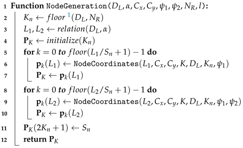
The structure is initially designed to change over time. Both the node position and the link orientation do not necessarily maintain constant values. The parameters were thought to manage the structure of nodes as a dynamic model. However, they remain subject to configuration within an external control scheme which could be governed, for example, by a DRL agent. As indicated by the algorithm shown in Algorithm 1, the main function for the dynamic generation of nodes, NodeGeneration(), is based on Equations 2 and 3, where the set of positions for each node is computed from the swarm center . Since each link contains a number of nodes that is not necessarily equal, the computation is performed independently through the procedures NodeCoordinates() based on Equation 2, and NodeCoordinates() based on Equation 3, respectively. In both cases, the resulting structure is concatenated into the final structure . Subsequently, it is reshaped into a one-dimensional vector, and the inter-node distance is appended at the final position. The NodeGeneration function is designed to have a dynamic output size, which implies that the number of nodes generated over time will be variable. It is important to refer that are calculated only once at beginning of the algorithm. As will be mentioned later, this variables are initially defined as the average position of all robots and its change will be calculated by the swarm dynamic model.
| Algorithm 1: Node Generation Function |
|
Input: Parameters , l. Variables , , , , , .
Output: Set of node coordinates .
 |
2.2. Swarm Node Cohesion
Once the nodes have been created, each exerts an attractive potential force on a specific number of units within the total robots . This attractive field does not involve all swarm members. The objective of the potential force is to group a specified number of robots around an assigned node. Based on its current position, each robot will be assigned a node around which it must position itself. In this manner, the potential influence directly affects the swarm’s pattern formation by using the node positions as uniformly distributed meet points. The number of robots influenced by a specific node is equivalent to (robots per node). From this approach, the swarm is equally distributed based on the shortest distance between robot and the nearest node position . Thus, the APF generated for each node is expressed as follows:
subject to:
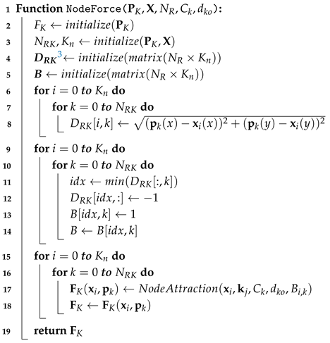
where represents the node attractive constant; denotes the value of the -th index within the assignability matrix B and represents the equilibrium distance. As shown in Equations 9 and , the potential force assigned to robot with respect to node depends entirely on the assignability factor which is activated based on the distance between and . As Equation 11 denotes, if the i-th unit is part of the robots with the minimum length toward the node, the assignability factor is equal to 1. At the same time, the function uniformly distributes the population of each node into a number of units at any given moment. This implies that even during abrupt formation changes, where robots are reassigned, the population at each node will remain constant. The global pattern formation will depend on potential force of each node. Simultaneously, is subject to the configuration of the PLN structure (i.e., under the formation control parameters). As Algorithm 2 shows, the NodeForce function is responsible for generate the set of node-influenced forces for all robots in the swarm. Based on the size of , an empty multi-dimensional vector is initialized; and are calculated based on all robot position vector , which refers to set of position vectors for all swarm members, and respectively; the distance matrix is initialized as an empty variable as well as the assignability matrix B. Next, the internal distance matrix between nodes and robots is filled with the calculated distances between robots and nodes. Based on the calculated matrix, the assignability matrix B is computed. Finally, derived from Equation 9 the procedure NodeAttraction is executed resulting in a force vector which will be part of the set of forces .
| Algorithm 2: Node Assignment Procedure |
|
Input: Parameters , , . Variables , .
Output: Set of force vectors under node’s influence .
 |
However, this method could produce inefficient behaviors such as jittering or thrashing due to frequent reassignment based solely on instantaneous proximity. This scenario is often related to collective rest configurations. It refers to the constant unnecessary reassignment when robots reach a nearly cohesive stable formation. In order to develop an efficient node assignment method when the swarm is near to rest (when robots has reach the vicinity of their assigned node), a persistent assignation mode can be considered. Assuming an persistent activation variable as:
where the assignment indicator defines the persistent assignment of robot i to a predefined node k at time t, is the neighborhood limit of node k and is the Euclidean distance between robot i and node k. In this mode, the robot would be only assigned to the last nearest node avoiding a constant node reassignment.
2.3. Attractive and Repulsive Artificial Potential Fields for Cohesiveness
In order to establish a cohesion influence dedicated to maintaining a unified swarm structure, each robot within the group is affected by an attractive force. The strength of the resulting force enables the swarm to remain cohesive during both motion and rest. This attractive-based cohesion component considers a specific swarm member with respect to others. The consequent sum of attractive forces determines the i-th robot’s orientation in order to preserve it in cohesion. The resultant attractive force acting on a robotic unit i with respect to another j can be expressed as follows:
where represents the cohesive-attractive constant and represents the equilibrium distance between the robot i and robot j respectively. This force is active among all robots in the swarm, excluding the same unit. However, as well as the attraction component brings units closer together, it does not generate an active collision avoidance. Even if decreases as tends to , the force does not have the potential to respond fast enough when the collision boundaries have been exceeded. To keep a safe distance between all members an active repulsion force is necessary. Therefore, with the aim to deal with collision and possible stuck due to local minima commonly encountered in traditional APF models, the total repulsive force is defined as the sum of both repulsion-based cohesion force and local minima escape force in the form . Initially, the repulsion-based cohesion force is generated by swarm when at least two robots are too close to each other or when a robot approaches a prior detected obstacle. This force is activated when the maximum allowable distance between robot i and robot-obstacle j is exceeded. It can be expressed as follows:
where represents the repulsive-cohesion constant, represents the minimum collision limit between the robot i and robot-obstacle j. The model used is based on [25,69] and guarantees the collision avoidance between all swarm members. As shown in Figure 4, is only active when distance between any two robots is less than . Furthermore, even if the repulsive force is usually prioritized in robotic swarms to avoid internal and external collision. The influence of repulsive force in Equation 15 is directly subjected to both constant gain and the distance , respectively. Finally, based on the Wall Following (WF) algorithm [70,71], the local minima escape force is defined as an additional repulsive force only activated when a robot detect it is in close proximity to an obstacle boundary. This selective force can be defined as:
where is a local minima escape constant, represents the safe distance between the robot i and the detected wall e, the unit direction vector between robot and the wall is defined as . Then, is the tangent vector that robot defines along the wall surface and is the tuning parameter regarding this tangential motion component. It must be emphasized that the value of can be assumed in Equation . However, implementation phases could involve data collection processes by onboard distance sensors or real-time mapping.
2.4. Attractive and Repulsive Stability
Lemma: Consider the system with the potential function composed of an attraction and a repulsion component , where and are the attractive and repulsive potential [69,72,73], respectively. This artificial fields are defined as:
where is the center of the obstacle with radius r and scaling . Then, the equilibrium point at is stable in the sense of Lyapunov.
Proof:
1. Lyapunov candidate function: We choose the total potential as the Lyapunov function and assuming the origin is outside the obstacle region.
2. Positive definiteness: By construction, for all . The repulsive potential since it is squared and vanishes outside the obstacle influence. Thus,
3. Time derivative of V: The system evolves as , taking the time derivative of along trajectories:
4. Stability conclusion: Since is positive definite and , Lyapunov’s direct method implies stability of the equilibrium at . If the set where contains only the equilibrium, then the equilibrium is asymptotically stable by LaSalle’s invariance principle.
The resultant expression validates the Lyapunov stability and secures the safety guarantee.
3. Differential Motion Transformation
As Section 2 refers, the resulting sum of forces represents the necessary alignment and proportional magnitude to maintain the robots in formation and cohesive. To make the swarm move following the information of , this set of vectors must be converted into motion through scalar velocities. Originally used in [25], the motion transformation system is simplified to turn a force vector into a linear u and angular velocity w respectively. However, the model is often subject to "involuntary collisions" caused by the effect of the repulsive force when a collision is detected. The MIMC-VADOC system drives the robot forward only, as it is designed to control differential-drive robots. It causes both velocities (linear and angular) are often activated simultaneously, which tends to cause collisions when the robot attempts to move out from another or from the detected obstacle’s boundary. Therefore, oscillations caused by the potential interaction between cohesive force and repulsive force in the APF approach may lead to a collective destabilization, moving the robots away from their nodes. To overcome such drawback, a repulsive limiter is applied to the linear velocity. This approach is based on the sigmoid activation function, which is given by:
where will be part of the repulsive limiter for the transformation system. In order to keep a vector notation, the robot’s current orientation , is defined as:
where can be computed as an alignment vector, simplifying the notation of the equation. Based on Eq. 22 and Eq. 23, the repulsive transformation model for each robot can be expressed as:
where the vector is the robot’s current alignment unitary value and is the orientation unitary vector of force. Additionally, is defined as the maximum available linear velocity of the robot and is the angular constant gain. The virtual angular distance is represented as follows:
where . This model enables a smooth exit for the robot when it is near collision boundaries. It is effective in prioritizing the redirection of robot until it can align with the nearest exit path.

Table 1.
Parameters used to set the cohesive PLN formation structure.
| Control Category | Parameter | Description | Influence |
|---|---|---|---|
| Cohesiveness | Node’s attractive coefficient | APF’s for nodes | |
| Node equilibrium distance | APF’s for nodes | ||
| Cohesive-attractive coefficient | APF’s for attraction | ||
| Attractive equilibrium distance | APF’s for attraction | ||
| Cohesive-repulsive coefficient | APF’s for repulsion | ||
| Repulsive minimum distance | APF’s for repulsion | ||
| Formation | Total structure length | PLN kinematics | |
| Length factor | PLN kinematics | ||
| First link direction | PLN kinematics | ||
| Second link direction | PLN kinematics | ||
| Swarm lineal velocity | PLN dynamics | ||
| Swarm angular velocity | PLN dynamics |
4. Simplified Collective Dynamics
To induce collective motion within the swarm, a simplified dynamic model is used to control the overall translation of the group. As outlined in Section 2.1, the reference point for calculating the swarm center is defined at . The group’s global motion is given by a set of dynamic inputs representing its linear and angular velocities. The system dynamics are formulated as follows:
where and are the states of the simplified dynamical system defined as swarm linear and angular velocity vectors respectively. Additionally, , and are calculated based on the collective average position and orientation. Thus, the PLN structure center from Equation 2 is updated dynamically by the swarm dynamic model based on the collective linear velocity and angular velocity evolving over time in the form:
where represents the instantaneous swarm velocity vector derived from and . As long as and are the swarm linear and angular scalar velocities, is the unitary direction vector of the swarm. Finally, is denoted by the alignment degree of the entire group, which is given by:
The degree of alignment among the swarm members directly influences the velocity of the collective motion at the swarm center. In the proposed model, misalignment among individual robots imposes constraints on the overall translational velocity, effectively limiting the group’s motion efficiency when deviations from the target heading occur.
5. Cohesiveness Evaluation
Evaluation of swarm’s cohesiveness involves applying an appropriate measurement method which considers the position of all members. For example, although Figure 5 shows evident modifications in response to changes in both node’s attractive coefficient and cohesive-attractive coefficient , this variations must be quantified. In this context, the density of the swarm (i.e., the number of robots in a given area) turns into an important concept to evaluate the group’s unity. To achieve this, non-parametric techniques have been chosen for density estimation. From [74], it is assumed a positional vector that contains the coordinates of n mobile robots. Consequently, the estimated probability of robots in to fall in a region is given by:
where is the volume enclosed by each from a sequence of regions . Each region contains samples and results in the probability .
In order to obtain the sequence of regions, the Parzen-Windows method is applied to estimate the density for each one. Assuming the region as a d-dimensional hypercube, the hypercube’s length of edge is defined as . In such wise, it is possible to obtain an expression for by counting the number of samples falling in the hypercube. The resultant window function procedure is defined as:
where defines a unit hypercube centered at the origin. This establishes that is equal to 1 if falls inside the hypercube’s volume centered at . Through window function can be calculated by:
Substituting Eq. 33 in Eq. 31, it is possible to develop a more general approach to estimate the density function, as follows:
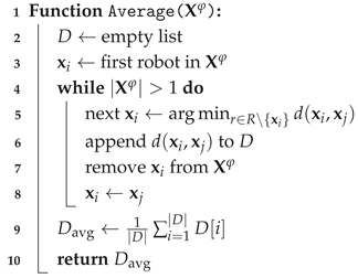
Then, the estimated density function is calculated for each Parzen window on a delimited plane. Finally, the average estimated density is calculated considering only non-zero density regions. Although a cohesive group is expected to have a high probability value , this result is not enough to evaluate a group under constraints of formation patterns and collision avoidance boundaries. In this scenario, it would be useful to measure the collective interspace value. However, the average distance between robots is a variable whose accurate measurement can be challenging. In large groups, the global average distance does not accurately represent the actual separation between two cohesive robots located on opposite edges of the swarm. In order to estimate the real average distance between robots, a PW-based resultant vector that contains the coordinates of robots inside the hypercube with a length of edge is defined as . Consequently, the mean distance between robots can be calculated as:
where represents the distance between robots and within the Parzen window. At each step, Eq. 35 removes the current robot from until only the last robot remains. As detailed in Algorithm 3, the Average() function provides a robust estimation of the swarm’s inter-robot distances. Consequently, the average swarm density and the mean inter-robot distance were analyzed from Figure 5. Figure 6 shows that high node-generated forces lead to lower swarm density. Conversely, under low cohesive-attraction constraints, the swarm preferentially aggregates around the formation nodes. While this behavior supports the required pattern formation, it can also result in undesirable proximity among robots, approaching the repulsion limits and potentially increasing collision risk.
| Algorithm 3: Average distance function |
|
Input: Parameters .
Output: Group’s average distance .
 |
6. Experimental Setup and Results
This section outlines the experimental setup used to test and validate the proposed collective model, along with the results obtained from two swarm coordination tests. Additionally, it presents a comprehensive evaluation of the PLN approach through multiple experimental trials, providing both qualitative and quantitative assessments. The experimental environment was developed and implemented using MATLAB R2023b (MathWorks®, Natick, MA, USA) and Simulink. Simulations were conducted with varying numbers of robots to study condensation and cohesion of the robot formation, as well as to assess the influence of local APF parameters and global swarm control variables on formation shape. Furthermore, the automatic generation of nodes was systematically evaluated using predefined functions within the simulation framework.
6.1. Performance Assessment for Aggregation Behavior
In order to evaluate the PLN-based formation system, the tests were conducted by adjusting the cohesiveness and formation parameters under aggregation constraints (i.e., the swarm is defined as stationary). For all tries in Figure 7, the robot’s distance between wheels was defined as [m] and the wheel radius is defined as [m]. As long as swarm does not present collective motion in these tests (i.e., aggregation behavior refers only to gathering), swarm’s linear and angular velocities are defined as and , respectively. In contrast, these sets of trials were designed to assess the group’s formation pattern response under cohesive parameter tuning, as Figure 7 illustrates. All tests were performed with 40 mobile differential robots on a two-dimensional space of meters. In trials (a), (b) and (c), cohesive parameters remained constant while the PLN structure was varied. The first three trials were cohesively adjusted based on responses from Section 5. Stable cohesion that does not significantly compromise the pattern formation, was observed on the relation . Following this correlation, parameter values were defined as and . In contrast, the trial (d) was performed under different cohesive values (, , ). In addition, (a), (b) and (c) were adjusted with different formation parameters in order to evaluate the swarm’s aggregation behavior under differentiated gathering points. The remaining parameter for this section can be found in Table 2. As Figure 7 shows, the target formation pattern for all trials is explicit. Although the four formations are successfully achieved, the simulation conditions focus not only on pattern configuration but also on cohesion adjustment (trial (d)). Based on results of cohesion analysis from Figure 8, a cohesive stability is reached approximately in (i.e., when mean density estimation and mean distance turn on stable). As an APFs based formation scheme, it is expected that the swarm tends to avoid repulsion boundaries. In contrast, if the group is cohesive, it is anticipated that the group leans to follow the attractive equilibrium distance . As mentioned above, trials (a)-(d) were performed with constant cohesive parameters previously analyzed in Section 5. These tests demonstrate the respective attraction distance tracking and repulsive boundary avoidance. Conversely, trial (d) was simulated with a higher node’s attractive coefficient . Although it was expected to achieve a more node-condensed behavior as the relation from Figure 5, this trial was setup with a different repulsive minimum distance [m] and an attractive equilibrium distance [m] respectively. The result obtained refers to a lower dense formation with a more covered space. The mean density estimation of this trial is lower with respect to others, while attractive distance tracking is not achieved. Moreover, the robots tend to approach close to the repulsive limits. This behavior implies the need for cohesive parameter re-adjustments when potential collective distances are modified. However, it also means that the swarm would be cohesively flexible with an appropriate parameter setting. Consequently, these initial experiments demonstrate successful pattern formation under conditions without collective CM.
6.2. Performance Assessment for Flocking Formation
In this section, the cohesion-based PLN structure is evaluated under active collective CM. These tests can be seen in Figure 9 and consists of four experiments with similar cohesion parameters based on the relation (). However, this time the swarm is explicitly stimulated with dynamic angular and linear velocity ( and ) respectively. These experiments were developed with swarm features similar to Section 6.1 ( [m], [m] and 40 robots). Regarding pattern formation, trials (a) and (d) were configured in a straight line arrangement while trials (b) and (c) had an triangular-shaped formation. In contrast, the first two tests were set with only linear velocity (i.e., and ), as long as the next two had active linear and angular velocities. In addition, dynamic formation changes were developed in tests (c) and (d). In (c), a time-based change function was formulated for the orientation of the first link . Similarly, the function was set for trial (d). All these parameters can be found in Table 3. Then, based on the results shown in Figure 10, a more irregular response is denoted while the group tries to keep the structure cohesive. Due to active collective CM, smooth cohesive stabilization is not expected as in the previous Section 6.1. In contrast, these tests were designed to assess pattern formation while the swarm is in motion (i.e., formation-based flocking behavior). The PLN system allows for configurable linear pattern structures which were adjusted with different parameters for each trial. Test (a) and (b) demonstrate an appropriate formation under active collective linear velocity as long as the PLN structure remains static. However, trials (c) and (d) show the swarm’s response in presence of simultaneously both collective angular/linear velocities and ongoing changes of the PLN structure. Furthermore, although Figure 10 demonstrates a lower mean density estimation of trials (a) and (d) with respect to (b) and (c), all experiments exhibit a respective tracking around [m] while no trial crosses the repulsive boundaries. These results shows a stable flocking transition for each test. Additionally, the obtained responses in Figure 10 suggest that mean density estimation is related with specific formation patterns. A lower density is expected for linear-shaped formation (i.e., more dispersed patterns) with respect to more grouped forms (i.e., close nodes formations).
Otherwise, an external obstacle avoidance trial was performed in Figure 11. These tests were set with a static PLN structure and a constant collective linear velocity [m/s]. The trial (a) was configured with a circular obstacle in position with 0.2 meters in diameter. In contrast, test (b) had two obstacles at positions and , respectively. Both results show the corresponding initial aggregation and the subsequent flocking behavior of the swarm. Additionally, (a) and (b) demonstrate the expected avoidance of collisions with respect to external obstacles. Although an initial pattern deformation around the obstructions is evident, the swarm achieves to rebuild the respective cohesion just after leaving the obstacle’s boundaries. An additional experiment was performed to evaluate the cohesive PLN structure for large groups. Due to previous tests that were configured with a constant robot number , Figure 12 demonstrates the behavior of the cohesive scheme for groups composed by and robotic units in (a) and (b), respectively. The PLN structure of trial (a) was spread in a triangle-shaped formation over 80 seconds. Although some cohesion deformation is evident in the final steps of the simulation, the results obtained demonstrate the preservation of the expected formation through the trial. This test was configured with cohesion parameters similar to those in Figure 9. In contrast, the result obtained from (b) shows a linear-shaped structure with a greater number of units. In this case, the formation obtained has a lower density and a larger covered area. Similarly to the previous, some pattern deformations can be seen in the final stages. However, the group is able to maintain the linear formation while the entire swarm is in motion. This experiment was set with a cohesive-node relation of (see Section 5) and with equilibrium distances of and for cohesive-attractive and cohesive-repulsive distances, respectively.
6.3. Tuning-Based Performance
To address concerns about potential oscillations arising from the interaction between the attractive force and the repulsive force , we conducted a series of simulation tests designed to evaluate the dynamic stability of the PLN system under variations of key gain parameters. Consequently, as Figure 13 four distinct trials were developed.
As Trial (a) shows, the node attractive gain was adjusted dynamically in real-time using a positive ramp signal during the interval to seconds within a total test duration of 60 seconds. The gain was increased by 200% relative to its initial value to observe the system response to enhanced node attraction. Next, in Trial (b), the cohesion-attractive gain was varied similarly with a positive ramp signal resulting in a 300% increase over the original value to assess the impact of stronger cohesion forces on group stability. Contrarily, in Trial (c), the repulsive gain was decreased following a negative ramp signal, ultimately reducing to zero to simulate weakening or loss of collision avoidance capability. Finally, Trial (d) shows that all gains , and were adjusted simultaneously according to the signals described above to explore combined effects on stability. Each trial was evaluated based on three critical metrics: the cohesion-attractive limit representing the target equilibrium mean inter-robot distance, the repulsive limit regarded as a safety threshold to prevent collisions, and the node attractive limit used to assess preservation of the formation pattern. From the collected data, we extracted the mean group cohesion distance and mean distances between robots and their assigned nodes over time.
The obtained results in Figure 13 demonstrates that Trail (a) exhibited the highest stability. Despite robots tending to cluster closer around nodes with increased , the formation pattern remained intact and collision limits were respected. Thereby, Trial (b) demonstrated that increasing the cohesion gain led to stronger attractive forces that exceeded the repulsion threshold, resulting in collision events due to excessive crowding. Trial (c) showed that weakening the repulsive force allowed robots to approach too closely, causing early collisions and system instability. Finally, Trial (d) revealed that simultaneous gain adjustments yielded initially stable behavior, but rapidly degraded to collision risk as the repulsive potential weakened relative to attraction forces.
Therefore, as Figure 14 shows, the sigmoid-based repulsive limiter demonstrates a significantly reduced linear velocity oscillations which should be directly related to a less energy consumption. The oscillation, caused by the potential interaction between cohesive force and repulsive force , may lead to a collective destabilization moving the robots away from their respective nodes. To mitigate this issues, a repulsive limiter is applied to the linear velocity. This approach is based on the sigmoid activation function. This model enables a smooth exit for the robot when it is near collision boundaries. It is effective in prioritizing the redirection of robot until it can align with the nearest exit path. The modification represent a more stable configuration of MIMC-based methods limiting the robot’s abrupt responses in boundaries of the attractive-repulsive potential fields. These findings highlight the critical importance of careful gain tuning to maintain dynamic stability and safe operation in swarm robotics applications, especially in real-world scenarios where persistent oscillations can increase energy consumption and mechanical wear.
7. Agriculture Tests
This section presents experimental evaluations conducted in real agricultural field maps to assess the control performance of the swarm-formation strategy.
7.1. Swarm Formation Test in Crop Aisles
This trial was developed within a structured agricultural environment characterized by repetitive crop-row patterns, which were modeled as static obstacle constraints, as illustrated in Figure 15. The virtual scenario was configured with five parallel crop corridors, each representing the navigable free space between adjacent rows. These corridors are typical physical restrictions faced by ground robots in precision agriculture tasks such as crop monitoring, spraying, or soil inspection, where the workspace is inherently narrow and elongated. At the initial stage, the swarm of mobile robots was spatially distributed into five subgroups, each assigned to one of the crop corridors. Every subgroup maintained a formation centered around PLNs that serve as local references regulating inter-robot distances and alignment. The robots move along the longitudinal axis of the field at a nearly constant speed of , producing a coordinated linear displacement across the different rows. This stage primarily evaluates the model’s ability to preserve intra-group cohesion and inter-row segregation, ensuring that each robot maintains its dynamic equilibrium under restricted maneuverability and proximity to environmental obstacles.
As the robots approached the terminal region of the crop field, they transitioned from a corridor-constrained configuration to an open-space aggregation phase. Upon exiting the row boundaries, the PLN-based control mechanism adapted to a global topology, where the influence of local reference nodes was progressively replaced by inter-agent potential coupling, guiding the robots toward a common meeting point. This transition demonstrates the capability of adaptive cohesion, enabling the swarm to autonomously shift from segmented linear flocking to a unified collective motion without requiring global synchronization or centralized supervision.
The emergent global flocking behavior highlights the PLN model’s robustness in dynamically varying environments. Actually, local interaction rules derived from potential-based coupling not only ensured collision-free navigation, but also preserved speed consensus and formation integrity throughout the maneuver. During the aggregation phase, the relative positional errors among nearby robots remained bounded within a 2–4% margin of the reference inter-agent distances, confirming stability under spatial reconfiguration. Overall, the experimental results demonstrate that the PLN model effectively maintains both local stability during structured navigation and global cohesion during cooperative aggregation. The model successfully reproduces the flocking behavior, transitioning smoothly from linear, row-constrained displacements to cohesive group convergence. Therefore, this trial validates the suitability for multi-robot coordination in motion control over agricultural scenarios, where decentralized control, obstacle avoidance, and dynamic topology adaptation are essential requirements for large-scale deployment.
7.2. Swarm Formation Test in Crop Fields
To further validate the applicability of the proposed PLN system in realistic agricultural environments, two new sets of simulation experiments based on 2D maps extracted from actual orchards in Chile were conducted.
The first experiment was developed using a map from the Melipilla region, Chile, an area characterized by agricultural fields with straight division lines and irregular angles (a typical layout in Chilean orchards). The field has a perimeter of approximately 4132.32 m and covers an area of 877,094.2 m2. The simulation deployed a swarm of 20 robots modeled after the dimensions of the AgriEco robot [36], each approximately 65 cm long and 55 cm wide, with a maximum velocity limited to 0.4 m/s. The robots were initially scattered within the northern portion of the map to simulate a realistic starting deployment scenario as Figure 16 shows. This setup tests the system’s performance over large, irregularly shaped crop fields commonly encountered in regional agriculture. As Figure 17 shows, the second experiment utilized a map extracted from an orchard in the Quillota region, Chile, which presents a more irregular crop distribution featuring curved and circular planting patterns. This orchard has a perimeter of 2496.49 m and an area spanning roughly 241,911.12 m2. The same robotic platform and number of units (20 robots) with identical velocity constraints were employed. Robots were initially placed in the northwest sector of the map to reflect operational constraints and starting locations typical in actual orchard management. This trial evaluates the system’s adaptability when navigating and coordinating in more complex and organic spatial configurations.
In both experiments, the repulsive limit distance was set to 68 cm, ensuring robots maintain safe separation to avoid collisions. The swarm cohesion distance was configured to 85 cm to promote close, coordinated motion without excessive crowding. Additionally, the node cohesion limit, which governs how tightly robots aggregate around formation nodes, was fixed at 30 cm. All artificial potential fields (APFs) gains were scaled based on the proportional relationships defined in Table 3, but amplified by a multiplication factor of 5.42 to adapt to the larger spatial scales and physical dimensions of the simulated orchards.
8. Discussion
8.1. Theoretical Methodology Analysis
It is important to mention that PLN framework is designed as a cohesive-formation structure able to be controlled by an unspecified control scheme. It means that PLN model is limited to manage the formation parameters (based on a configurable lineal kinematics and a simplified dynamic, respectively) and the structural cohesive configuration (based on APFs). In this scenario, the PLN scheme is not necessarily designed to reach a collective goal precisely, but rather to be the structural resource to achieve this requirement. It means the selected control model should be able to reach a specific goal point collectively by adjusting the kinematic, dynamic and cohesive parameters both in rest mode (aggregation) and in collective motion (flocking behavior). Due PLN system is focused on the structural integrity of a mobile group, collective and individual stable positions are expected (where some forces achieve a mutual cancellation). In fact, this state is necessary to preserve the cohesion in rest and flocking mode by the interaction between cohesive force and repulsion force . Additionally, given that node force is designed to shape and move the group collectively, the potential stable relationship between and defines the swarm final shape. It means either the pattern formation (assigning to a high value) or group cohesion (with a high value of ) can be prioritized. This implies the parameter adjusting process can define the structural configuration and transition of the PLN model. This is not only limited to a previous offline tuning procedure but a real-time parameter adjusting executed by a suitable controller.
Furthermore, the dynamic assignment approach (robot-to-node) seems to represent a flexible reassignment strategy that offers functional benefits aligned with the objectives of the PLN framework. By not rigidly binding a robot to a single node, the system enhances adaptability in pattern formation and collective motion. This flexibility allows the swarm to effectively respond to dynamic external obstacles and abrupt changes in formation patterns, thereby reducing the likelihood of collective clatter or deadlocks. By other side, even if this approach could produce inefficient behaviors such as jittering or thrashing due to frequent reassignment based solely on instantaneous proximity, this scenarios are only related to collective rest configurations. It refers to the constant unnecessary reassignment when robots reach a nearly cohesive stable formation. This scenario is explained in Section 2.2 and the persistent assignment method is described in Equation 12. In this mode, the robot would be only assigned to the last nearest node avoiding a constant node reassignment. However, this mechanism should be enhanced in presence of abrupt formation pattern changes and number of nodes. Given that both the node generation process and node positioning are managed by an external control scheme, a efficient reassignment method could represent a complex problem due the dynamic change of PLN system. In consequence, the robot-to-node assignment mechanism prioritize a equal robot distribution per node even in presence of unexpected formation changes.
Consequently, the obtained experimental results were developed by an off-line gain tuning procedure (APFs based constant gains). Some selected gain values were changed in the experiments to evaluate both the cohesive behavior and the collision avoiding, respectively. Regarding the collision avoidance, the PLN system employs two complementary mechanisms to prevent collisions despite the competing magnitudes of the attractive and repulsive forces. First, the dynamic robot-to-node assignment method promotes collision avoidance by reassigning robots to nodes based on relative proximity. Specifically, if a robot i is near another robot j but far from its assigned node k, robot j (being closer to node k) is more likely to be assigned to node k, while robot i is reassigned to a different node. This dynamic reassignment prevents multiple robots from converging on the same node, mitigating collision risks. Second, the system includes a sigmoid-based repulsive velocity limiter that reduces the linear velocity of a robot i as it approaches the boundaries of the repulsive force field generated by nearby robots or obstacles. This effectively forces the robot to slow down and maneuver safely around obstacles.
Finally, regarding the formation quality, it is important to clarify that when the cohesive attraction force is dominant, the swarm tends to form a circular aggregation with less adherence to node positions, compromising the prescribed formation pattern. Conversely, a stronger node attraction force causes robots to cluster tightly around the designated nodes, maintaining the pattern but potentially sacrificing overall swarm cohesion. This behavior can be clearly observed in Figure 5.
Our evaluation results suggest that the cohesion gain constant should be at least 40 times larger than the node attraction gain constant (as evidenced in experiments with 20, 40, and 60 robots). This ratio achieves a suitable balance, preserving the geometric formation while maintaining strong swarm cohesiveness.
8.2. Agriculture Application Analysis
Although robotic swarms hold significant promise as highly exploitable methods in agriculture, applied research remains relatively scarce. For example, [43] formulates the path planning challenge as a specialized Vehicle Routing Problem (VRP). While this work article and our study utilize satellite imagery and predefined meeting points for data collection, the primary distinction lies in their focus. The referenced work addresses UAV-based swarms with efficient aerial path planning, whereas our manuscript concentrates on UGV-based swarms designed to navigate and operate within obstacle-rich, structured ground environments. Contrarily, [57] targets fast and accurate path planning for agricultural information gathering robots in varied environments. It combines the global search capabilities of Particle Swarm Optimization and the local obstacle avoidance strengths of Ant Colony Optimization to optimize robot motion strategies. Their experiments, performed on grid-based environments using function-value-based optimization. In contrast, our PLN framework operates within more structured agricultural settings with pre-experiment offline tuning of control gains, maintaining constant gains in the presented trials. Importantly, PLN is compatible with advanced control schemes, including learning-based and optimal control methods, which we anticipate will be crucial to improving adaptability and robustness in future work.
Moreover, the PLN system, as a structural framework, does not incorporate an explicit optimization process. Instead, it provides a theoretical basis for collective formation and motion control. We acknowledge that realistic implementations must address practical challenges, such as the need for all-to-all communication or the deployment of complex consensus algorithms to ensure coordinated behavior across the swarm. Consensus algorithms, which enable decentralized agreement on shared objectives through local communication and peer-to-peer message passing, are central to achieving robust coordination in swarm robotics. Examples include average consensus, max-min consensus, and advanced distributed algorithms leveraging factor graphs and belief propagation, which have demonstrated scalability, resilience to communication failures, and efficiency in dynamic environments.
Despite these promising techniques, their integration introduces additional communication overhead and computational complexity, which can impose bottlenecks affecting scalability and real-time responsiveness. The PLN system presented in this manuscript is, therefore, intended as a partially decentralized theoretical proposal that lays the groundwork for further developments. Future work envisions incorporating such consensus-based distributed coordination methods and optimal control techniques to enhance the practical applicability of the PLN framework, enabling efficient, scalable, and robust swarm behaviors in complex, real-world agricultural environments.
9. Conclusions
This paper presented a cohesive-supported flocking model for robotic swarms based on cohesiveness stabilization through a APF-based collective formation structure in agricultural fields. The proposed model regulated swarm dynamics via a defined set of control parameters, distinguishing itself from other approaches by emphasizing global group behavior rather than direct individual interactions. The system was evaluated through extensive experimentation, involving stationary swarms (aggregation behavior), moving swarms (flocking behavior), robotic groups of varying sizes and agriculture row-crop based environment. The analysis focused on local cohesiveness around nodes within a Potential Linked Node model, as well as the overall swarm cohesion to ensure the construction of uniformed groups with specific formation patterns. Results obtained demonstrated that the proposed model effectively fulfils the target formation shape and avoids the inter-robot collisions. The developed system maintains cohesive stability across different swarm conditions (i.e., rest, motion, under presence of external obstacles, large group formation and segmented environments), preserving structural integrity during motion and under diverse formation configurations. The proposed system aimed at controlling the dynamic and kinematic characteristics of the swarm collectively with a set of simple configuration parameters to explore the development of complex behavior that do not necessarily require complex control systems. Furthermore, the PLN-based formations highlight the model’s adaptability, offering flexibility in regulating group cohesion while ensuring collision avoidance.
A key aspect of the proposed approach is to reinforce the notion that cohesion, as a fundamental control variable, can be used as a robust mechanism for shaping coordinated behaviors in large-scale mobile robotic systems. This work emphasizes the collective control through the adjustment of collective parameters in order to generate a simple unified model able to execute complex tasks in concept and agricultural scenarios.
Data Availability Statement
The original contributions presented in this study are included in the article. For further inquiries, please contact the corresponding author.
Acknowledgments
The authors thank the support of ANID under Fondecyt Iniciación en Investigación 2023 Grant 11230962.
Conflicts of Interest
The authors declare no conflicts of interest.
References
- Tan, Y.; yang Zheng, Z. Research Advance in Swarm Robotics. Defence Technology 2013, 9, 18–39. [Google Scholar] [CrossRef]
- Wang, F.; Fu, Q.; Hong, M.; Tang, W.; Su, L.; Zhu, D.; Wang, Q. Optimization of Cotton Field Irrigation Scheduling Using the AquaCrop Model Assimilated with UAV Remote Sensing and Particle Swarm Optimization. Agriculture 2025, 15. [Google Scholar] [CrossRef]
- Isaeva, V.V. Self-organization in biological systems. 39, 110–118. [CrossRef]
- Vittori, K.; Talbot, G.; Gautrais, J.; Fourcassié, V.; Araújo, A.F.R.; Theraulaz, G. Path efficiency of ant foraging trails in an artificial network. 239, 507–515. [CrossRef] [PubMed]
- Beshers, S.N.; Fewell, J.H. MODELS OF DIVISION OF LABOR IN SOCIAL INSECTS. Annual Review of Entomology 2001, 46, 413–440. [Google Scholar] [CrossRef] [PubMed]
- Czirók, A.; Vicsek, T. Collective motion. In Proceedings of the Statistical Mechanics of Biocomplexity; Reguera, D., Vilar, J., RubÃ, J., Eds.; Springer Berlin Heidelberg; pp. 152–164.
- Deutsch, A.; Theraulaz, G.; Vicsek, T. Collective motion in biological systems. 2012. [Google Scholar] [CrossRef]
- Ferrante, E.; Turgut, A.E.; Dorigo, M.; Huepe, C. Collective motion dynamics of active solids and active crystals. New Journal of Physics 2013, 15, 095011. [Google Scholar] [CrossRef]
- Raoufi, M.; Turgut, A.E.; Arvin, F. Self-organized Collective Motion with a Simulated Real Robot Swarm. In Proceedings of the Towards Autonomous Robotic Systems; Althoefer, K., Konstantinova, J., Zhang, K., Eds.; Cham; 2019; pp. 263–274. [Google Scholar]
- Schranz, M.; Umlauft, M.; Sende, M.; Elmenreich, W. Swarm Robotic Behaviors and Current Applications. Frontiers in Robotics and AI 2020, 7. [Google Scholar] [CrossRef]
- Arnold, R.; Carey, K.; Abruzzo, B.; Korpela, C. What is A Robot Swarm: A Definition for Swarming Robotics. In Proceedings of the 2019 IEEE 10th Annual Ubiquitous Computing, Electronics and Mobile Communication Conference (UEMCON), 2019; pp. 0074–0081. [Google Scholar] [CrossRef]
- Shahzad, M.M.; Saeed, Z.; Akhtar, A.; Munawar, H.; Yousaf, M.H.; Baloach, N.K.; Hussain, F. A Review of Swarm Robotics in a NutShell. Drones 2023, 7. [Google Scholar] [CrossRef]
- Antonyshyn, L.; Silveira, J.; Givigi, S.; Marshall, J. Multiple Mobile Robot Task and Motion Planning: A Survey. ACM Comput. Surv. 2023, 55. [Google Scholar] [CrossRef]
- Parker, L.E.; Rus, D.; Sukhatme, G.S. Multiple Mobile Robot Systems. In Springer Handbook of Robotics; Siciliano, B., Khatib, O., Eds.; Springer International Publishing: Cham, 2016; pp. 1335–1384. [Google Scholar] [CrossRef]
- Turgut, A.E.; Çelikkanat, H.; Gökçe, F.; Åžahin, E. Self-organized flocking in mobile robot swarms; 2, 97–120. [CrossRef]
- Ferrante, E.; Turgut, A.E.; Huepe, C.; Stranieri, A.; Pinciroli, C.; Dorigo, M. Self-organized flocking with a mobile robot swarm: a novel motion control method. Adaptive Behavior 2012, 20, 460–477. [Google Scholar] [CrossRef]
- Çelikkanat, H.; Åžahin, E. Steering self-organized robot flocks through externally guided individuals. 19, 849–865. [CrossRef]
- Khaldi, B.; Cherif, F. A Virtual Viscoelastic Based Aggregation Model for Self-organization of Swarm Robots System. In Proceedings of the Towards Autonomous Robotic Systems; Alboul, L., Damian, D., Aitken, J.M., Eds.; Cham; 2016; pp. 202–213. [Google Scholar]
- Santos, V.G.; Pires, A.G.; Alitappeh, R.J.; Rezeck, P.A.F.; Pimenta, L.C.A.; Macharet, D.G.; Chaimowicz, L. Spatial segregative behaviors in robotic swarms using differential potentials. 14, 259–284. [CrossRef]
- Misir, O.; Gökrem, L. Flocking-Based Self-Organized Aggregation Behavior Method for Swarm Robotics. 45, 1427–1444. [CrossRef]
- Soza Mamani, K.M.; Richard Díaz Palacios, F. Flocking Model for Self-Organized Swarms. In Proceedings of the 2019 International Conference on Electronics, Communications and Computers (CONIELECOMP), 2019; pp. 9–17. [Google Scholar] [CrossRef]
- Elkilany, B.G.; Abouelsoud, A.A.; Fathelbab, A.M.R.; Ishii, H. A proposed decentralized formation control algorithm for robot swarm based on an optimized potential field method. 33, 487–499. [CrossRef]
- Soza Mamani, K.M.; Saavedra Alcoba, M. Low-Computational-Load Real-time Path Planning and Trajectory Control based on Artificial Potential Fields. In Proceedings of the 2023 IEEE Colombian Caribbean Conference (C3), 2023; pp. 1–6. [Google Scholar] [CrossRef]
- Wang, S.; Zhang, J.; Zhang, J. Artificial potential field algorithm for path control of unmanned ground vehicles formation in highway. Electronics Letters 2018, 54, 1166–1168. [Google Scholar] [CrossRef]
- Mamani, K.M.S.; Ordoñez, J. MIMC-VADOC Model for Autonomous Multi-robot Formation Control Applied to Differential Robots. In Proceedings of the 2022 8th International Conference on Automation, Robotics and Applications (ICARA), 2022; pp. 118–124. [Google Scholar] [CrossRef]
- Souza, R.M.J.A.; Lima, G.V.; Morais, A.S.; Oliveira-Lopes, L.C.; Ramos, D.C.; Tofoli, F.L. Modified Artificial Potential Field for the Path Planning of Aircraft Swarms in Three-Dimensional Environments. Sensors 2022, 22. [Google Scholar] [CrossRef]
- Raibail, M.; Rahman, A.H.A.; AL-Anizy, G.J.; Nasrudin, M.F.; Nadzir, M.S.M.; Noraini, N.M.R.; Yee, T.S. Decentralized Multi-Robot Collision Avoidance: A Systematic Review from 2015 to 2021. Symmetry 2022, 14. [Google Scholar] [CrossRef]
- Rezaee, H.; Abdollahi, F. Mobile robots cooperative control and obstacle avoidance using potential field. In Proceedings of the 2011 IEEE/ASME International Conference on Advanced Intelligent Mechatronics (AIM), 2011; pp. 61–66. [Google Scholar] [CrossRef]
- Rezaee, H.; Abdollahi, F. A Decentralized Cooperative Control Scheme With Obstacle Avoidance for a Team of Mobile Robots. IEEE Transactions on Industrial Electronics 2014, 61, 347–354. [Google Scholar] [CrossRef]
- Zhao, J.; Fang, J.; Wang, S.; Wang, K.; Liu, C.; Han, T. Obstacle Avoidance of Multi-Sensor Intelligent Robot Based on Road Sign Detection. Sensors 2021, 21. [Google Scholar] [CrossRef]
- Yu, Y.; Wu, Z.; Cao, Z.; Pang, L.; Ren, L.; Zhou, C. A laser-based multi-robot collision avoidance approach in unknown environments. International Journal of Advanced Robotic Systems 2018, 15, 1729881418759107. [Google Scholar] [CrossRef]
- Al-Amin, A.A.; Lowenberg-DeBoer, J.; Franklin, K.; Dickin, E.; Monaghan, J.M.; Behrendt, K. Autonomous regenerative agriculture: Swarm robotics to change farm economics. Smart Agricultural Technology 2025, 11, 101005. [Google Scholar] [CrossRef]
- Nkwocha, C.L.; Adewumi, A.; Folorunsho, S.O.; Eze, C.; Jjagwe, P.; Kemeshi, J.; Wang, N. A Comprehensive Review of Sensing, Control, and Networking in Agricultural Robots: From Perception to Coordination. Robotics 2025, 14. [Google Scholar] [CrossRef]
- Hamrani, A.; Allouhi, A.; Bouarab, F.Z.; Jayachandran, K. AI and Robotics in Agriculture: A Systematic and Quantitative Review of Research Trends (2015–2025). Crops 2025, 5. [Google Scholar] [CrossRef]
- Albiero, D.; Pontin Garcia, A.; Kiyoshi Umezu, C.; Leme de Paulo, R. Swarm robots in mechanized agricultural operations: A review about challenges for research. Computers and Electronics in Agriculture 2022, 193, 106608. [Google Scholar] [CrossRef]
- Shi, Z.; Bai, Z.; Yi, K.; Qiu, B.; Dong, X.; Wang, Q.; Jiang, C.; Zhang, X.; Huang, X. Vision and 2D LiDAR Fusion-Based Navigation Line Extraction for Autonomous Agricultural Robots in Dense Pomegranate Orchards. Sensors 2025, 25. [Google Scholar] [CrossRef]
- Urrea, C. Hybrid Fault-Tolerant Control in Cooperative Robotics: Advances in Resilience and Scalability. Actuators 2025, 14. [Google Scholar] [CrossRef]
- Jiang, L.; Xu, B.; Husnain, N.; Wang, Q. Overview of Agricultural Machinery Automation Technology for Sustainable Agriculture. Agronomy 2025, 15. [Google Scholar] [CrossRef]
- Rasouli, S.; Dautenhahn, K.; Nehaniv, C.L. Simulation of a Bio-Inspired Flocking-Based Aggregation Behaviour in Swarm Robotics. Biomimetics 2024, 9. [Google Scholar] [CrossRef]
- Tarapore, D.; Groß, R.; Zauner, K.P. Sparse Robot Swarms: Moving Swarms to Real-World Applications. Frontiers in Robotics and AI 2020, 7–2020. [Google Scholar] [CrossRef]
- Botteghi, N.; Kamilaris, A.; Sinai, L.; Sirmacek, B. MULTI-AGENT PATH PLANNING OF ROBOTIC SWARMS IN AGRICULTURAL FIELDS. ISPRS Annals of the Photogrammetry, Remote Sensing and Spatial Information Sciences 2020, V-1-2020, 361–368. [Google Scholar] [CrossRef]
- David, C.N.A.; Yumol, J.V.; Garcia, R.G.; Ballado, A.H. Swarm Robotics Application for Gathering Soil Samples. In Proceedings of the 2021 IEEE 13th International Conference on Humanoid, Nanotechnology, Information Technology, Communication and Control, Environment, and Management (HNICEM), 2021; pp. 1–6. [Google Scholar] [CrossRef]
- Postmes, J.; Botteghi, N.; Sirmacek, B.; Kamilaris, A. A System for Efficient Path Planning and Target Assignment for Robotic Swarms in Agriculture. In Proceedings of the Proceedings of the 11th International Conference on the Internet of Things, New York, NY, USA, 2022; IoT ’21, pp. 158–164. [Google Scholar] [CrossRef]
- Dziomin, U.; Kabysh, A.; Golovko, V.; Stetter, R. A multi-agent reinforcement learning approach for the efficient control of mobile robot. Proceedings of the 2013 IEEE 7th International Conference on Intelligent Data Acquisition and Advanced Computing Systems (IDAACS) 2013, Vol. 02, 867–873. [Google Scholar] [CrossRef]
- Blais, M.A.; Akhloufi, M.A. Reinforcement learning for swarm robotics: An overview of applications, algorithms and simulators. Cognitive Robotics 2023, 3, 226–256. [Google Scholar] [CrossRef]
- Mamani, K.M.S.; Camacho, O.; Prado, A. Deep Reinforcement Learning Via Nonlinear Model Predictive Control for Thermal Process with Variable Longtime Delay. In Proceedings of the 2024 IEEE ANDESCON 2024, 1–6. [Google Scholar] [CrossRef]
- Rajasekhar, N.; Radhakrishnan, T.K.; Mohamed, S.N. Reinforcement learning based temperature control of a fermentation bioreactor for ethanol production. Place: United States 121, 3114–3127. [CrossRef] [PubMed]
- Yan, P.; Bai, C.; Zheng, H.; Guo, J. Flocking Control of UAV Swarms with Deep Reinforcement Leaming Approach. In Proceedings of the 2020 3rd International Conference on Unmanned Systems (ICUS), 2020; pp. 592–599. [Google Scholar] [CrossRef]
- Cao, Y.; Ni, K.; Jiang, X.; Kuroiwa, T.; Zhang, H.; Kawaguchi, T.; Hashimoto, S.; Jiang, W. Path following for Autonomous Ground Vehicle Using DDPG Algorithm: A Reinforcement Learning Approach. Applied Sciences 2023, 13. [Google Scholar] [CrossRef]
- Zhou, J.; Zhang, H.; Hua, M.; Wang, F.; Yi, J. P-DRL: A Framework for Multi-UAVs Dynamic Formation Control under Operational Uncertainty and Unknown Environment. Drones 2024, 8. [Google Scholar] [CrossRef]
- Dong, Z.; Tan, F.; Yu, M.; Xiong, Y.; Li, Z. A Bio-Inspired Sliding Mode Method for Autonomous Cooperative Formation Control of Underactuated USVs with Ocean Environment Disturbances. Journal of Marine Science and Engineering 2024, 12. [Google Scholar] [CrossRef]
- Tuzel, O.; Fleming, C.; Marcon, G.H. Learning Flocking Control in an Artificial Swarm. 2017. [Google Scholar]
- Martinez, F.; Montiel, H.; Wanumen, L. A deep reinforcement learning strategy for autonomous robot flocking. International Journal of Electrical and Computer Engineering (IJECE) 2023, 13, 5707–5716. [Google Scholar] [CrossRef]
- Bezcioglu, M.B.; Lennox, B.; Arvin, F. Self-Organised Swarm Flocking with Deep Reinforcement Learning. In Proceedings of the 2021 7th International Conference on Automation, Robotics and Applications (ICARA), 2021; pp. 226–230. [Google Scholar] [CrossRef]
- Chen, L.; Zhao, Y.; Zhao, H.; Zheng, B. Non-Communication Decentralized Multi-Robot Collision Avoidance in Grid Map Workspace with Double Deep Q-Network. Sensors 2021, 21. [Google Scholar] [CrossRef]
- Na, S.; Niu, H.; Lennox, B.; Arvin, F. Bio-Inspired Collision Avoidance in Swarm Systems via Deep Reinforcement Learning. IEEE Transactions on Vehicular Technology 2022, 71, 2511–2526. [Google Scholar] [CrossRef]
- Wu, Q.; Chen, H.; Liu, B. Path Planning of Agricultural Information Collection Robot Integrating Ant Colony Algorithm and Particle Swarm Algorithm. IEEE Access 2024, 12, 50821–50833. [Google Scholar] [CrossRef]
- Zhang, Y.; Oğuz, S.; Wang, S.; Garone, E.; Wang, X.; Dorigo, M.; Heinrich, M.K. Self-Reconfigurable Hierarchical Frameworks for Formation Control of Robot Swarms. IEEE Transactions on Cybernetics 2024, 54, 87–100. [Google Scholar] [CrossRef] [PubMed]
- Zhu, W.; Oğuz, S.; Heinrich, M.K.; Allwright, M.; Wahby, M.; Christensen, A.L.; Garone, E.; Dorigo, M. Self-organizing nervous systems for robot swarms. Science Robotics 2024, 9, eadl5161. [Google Scholar] [CrossRef] [PubMed]
- Yao, Q.; Zheng, Z.; Qi, L.; Yuan, H.; Guo, X.; Zhao, M.; Liu, Z.; Yang, T. Path Planning Method With Improved Artificial Potential Field—A Reinforcement Learning Perspective. IEEE Access 2020, 8, 135513–135523. [Google Scholar] [CrossRef]
- Li, L.; Wu, D.; Huang, Y.; Yuan, Z.M. A path planning strategy unified with a COLREGS collision avoidance function based on deep reinforcement learning and artificial potential field. Applied Ocean Research 2021, 113, 102759. [Google Scholar] [CrossRef]
- Nouyan, S.; Campo, A.; Dorigo, M. Path formation in a robot swarm. 2, 1–23. [CrossRef]
- Bautista, J.; de Marina, H.G. Behavioral-based circular formation control for robot swarms. In Proceedings of the 2024 IEEE International Conference on Robotics and Automation (ICRA), 2024; pp. 8989–8995. [Google Scholar] [CrossRef]
- Lee, G.; Chong, N.Y.; Christensen, H. Adaptive triangular mesh generation of self-configuring robot swarms. In Proceedings of the 2009 IEEE International Conference on Robotics and Automation, 2009; pp. 2737–2742. [Google Scholar] [CrossRef]
- Shirazi, A.R.; Jin, Y. A Strategy for Self-Organized Coordinated Motion of a Swarm of Minimalist Robots. IEEE Transactions on Emerging Topics in Computational Intelligence 2017, 1, 326–338. [Google Scholar] [CrossRef]
- Jadhav, V.; Guttal, V.; Masila, D.R. Randomness in the choice of neighbours promotes cohesion in mobile animal groups. Royal Society Open Science 2022, 9, 220124. [Google Scholar] [CrossRef]
- Lee, S.K. Distributed cohesive configuration controller for a swarm with low-cost platforms. Journal of Field Robotics 2023, 40, 30–56. [Google Scholar] [CrossRef]
- Yigit, B.; Alapan, Y.; Sitti, M. Cohesive self-organization of mobile microrobotic swarms. Soft Matter 2020, 16, 1996–2004. [Google Scholar] [CrossRef]
- Khatib, O. Real-time obstacle avoidance for manipulators and mobile robots. In Proceedings of the Proceedings. 1985 IEEE International Conference on Robotics and Automation 1985, Vol. 2, 500–505. [Google Scholar] [CrossRef]
- Mabrouk, M.H.; McInnes, C.R. Wall following to escape local minima for swarms of agents using internal states and emergent behaviour. In Proceedings of the International Conference on Computational Intelligence and Intelligent Systems, ICCIIS 08, 2008; International Association of Engineers; pp. 24–31. [Google Scholar]
- Kim, J.; Park, S.; Lee, W.; Kim, W.; Choi, H.; Doh, N.; Nam, C. Escaping Local Minima: Hybrid Artificial Potential Field with Wall-Follower for Decentralized Multi-Robot Navigation. In Proceedings of the 2025 IEEE International Conference on Robotics and Automation (ICRA), 2025; pp. 6616–6622. [Google Scholar] [CrossRef]
- Singletary, A.; Klingebiel, K.; Bourne, J.; Browning, A.; Tokumaru, P.; Ames, A. Comparative Analysis of Control Barrier Functions and Artificial Potential Fields for Obstacle Avoidance. In Proceedings of the 2021 IEEE/RSJ International Conference on Intelligent Robots and Systems (IROS), 2021; pp. 8129–8136. [Google Scholar] [CrossRef]
- Melchiorre, M.; Salamina, L.; Scimmi, L.S.; Mauro, S.; Pastorelli, S. Experiments on the Artificial Potential Field with Local Attractors for Mobile Robot Navigation. Robotics 2023, 12. [Google Scholar] [CrossRef]
- Duda, R.O.; Hart, P.E.; et al. Pattern classification; John Wiley & Sons, 2006. [Google Scholar]
Figure 1.
A set of robots performing formation tasks, typically required in agricultural settings.
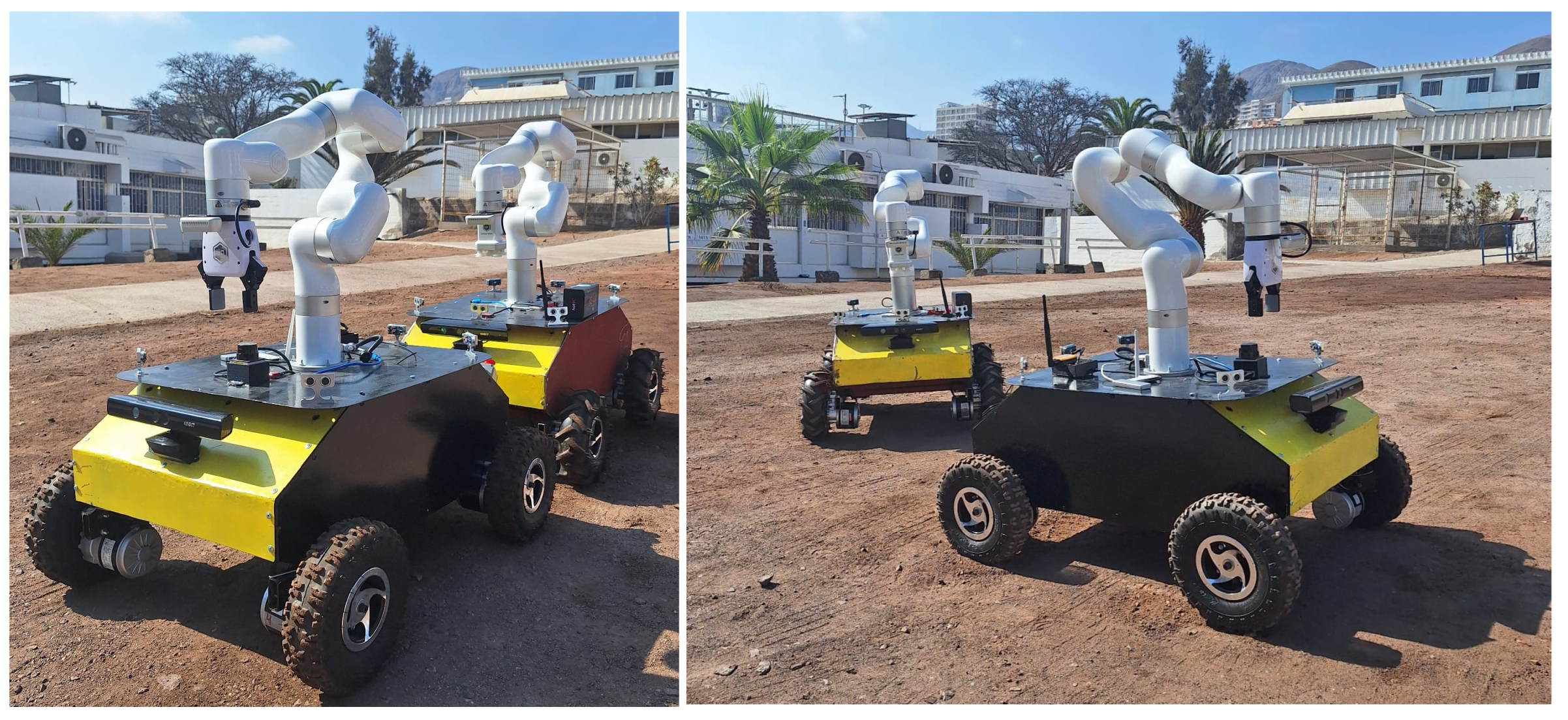
Figure 2.
Diagram of cohesive swarm managing through potential forces.
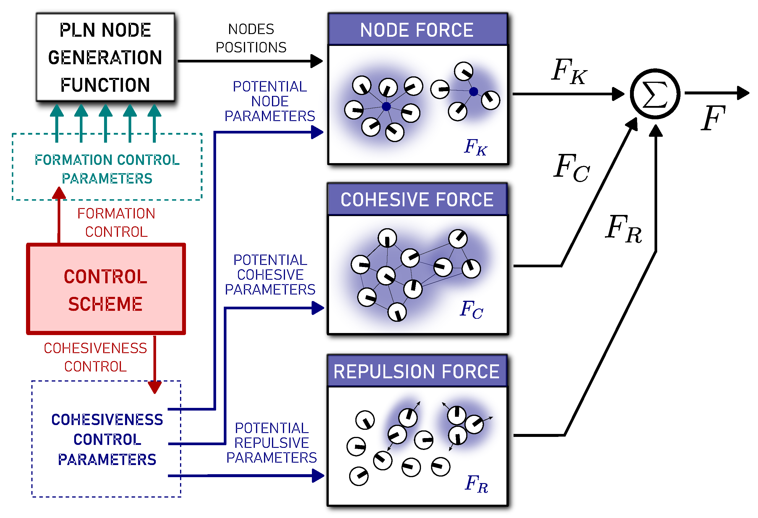
Figure 3.
Basal configuration for node orientation and positioning on the PLN system for robot formation.
Figure 3.
Basal configuration for node orientation and positioning on the PLN system for robot formation.
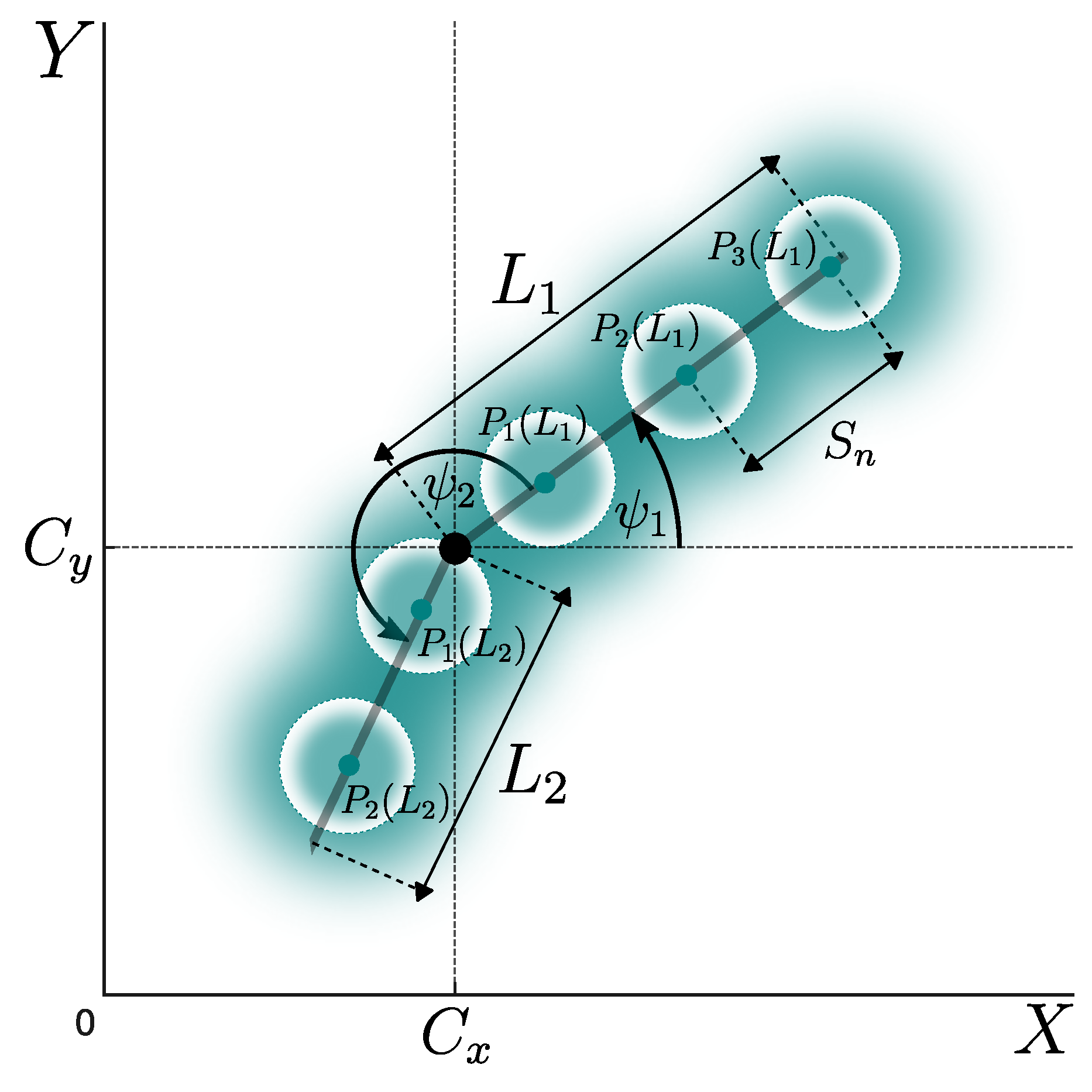
Figure 4.
Diagram of APF’s forces over the entire robotic swarm.
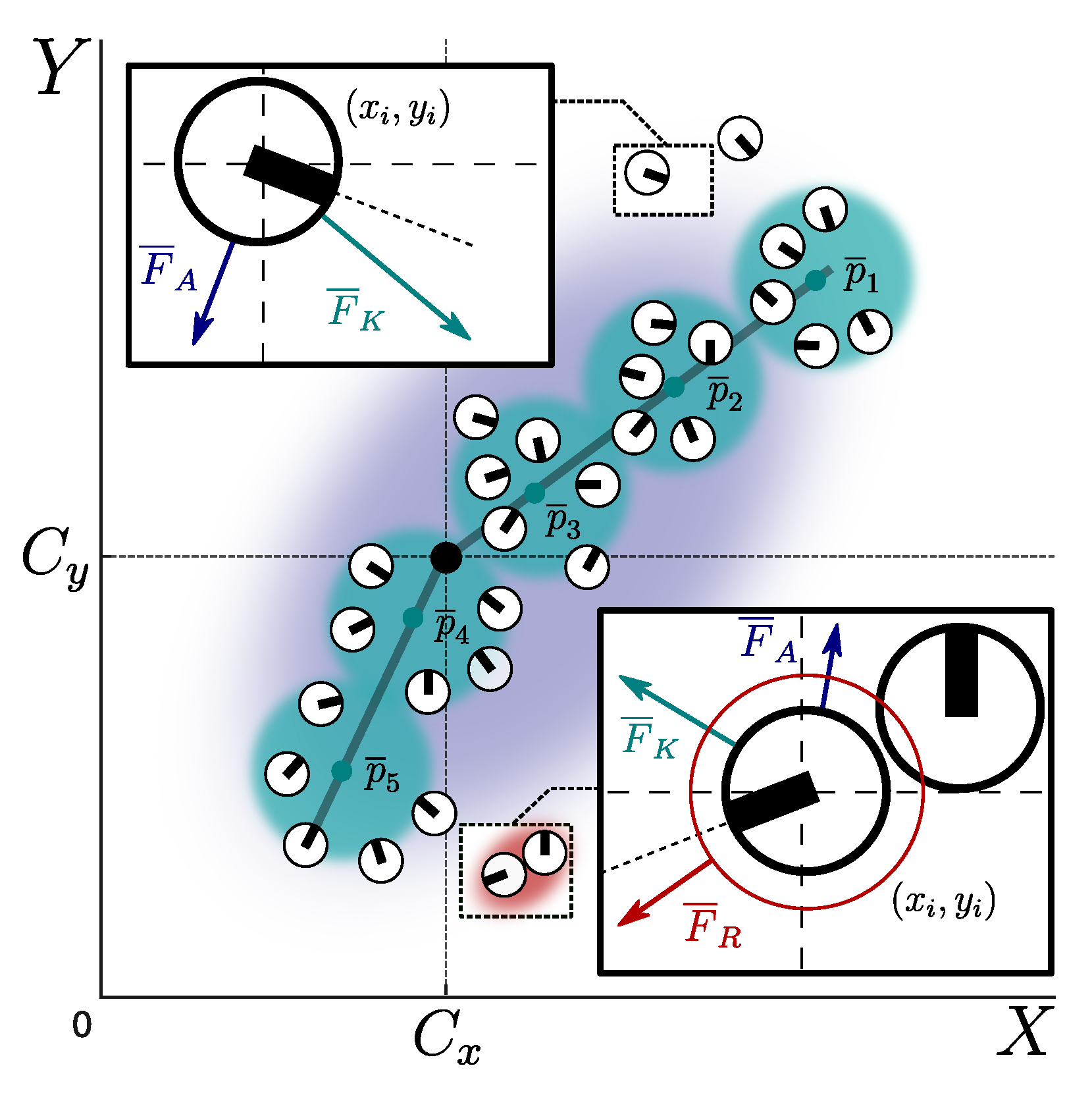
Figure 5.
Global cohesion analysis of the robotic swarm under variations of the node’s attractive coefficient and the cohesive-attractive coefficient . The swarm density is estimated using a non-parametric method to quantify changes in spatial unity and group cohesion in response to the parameter adjustments.
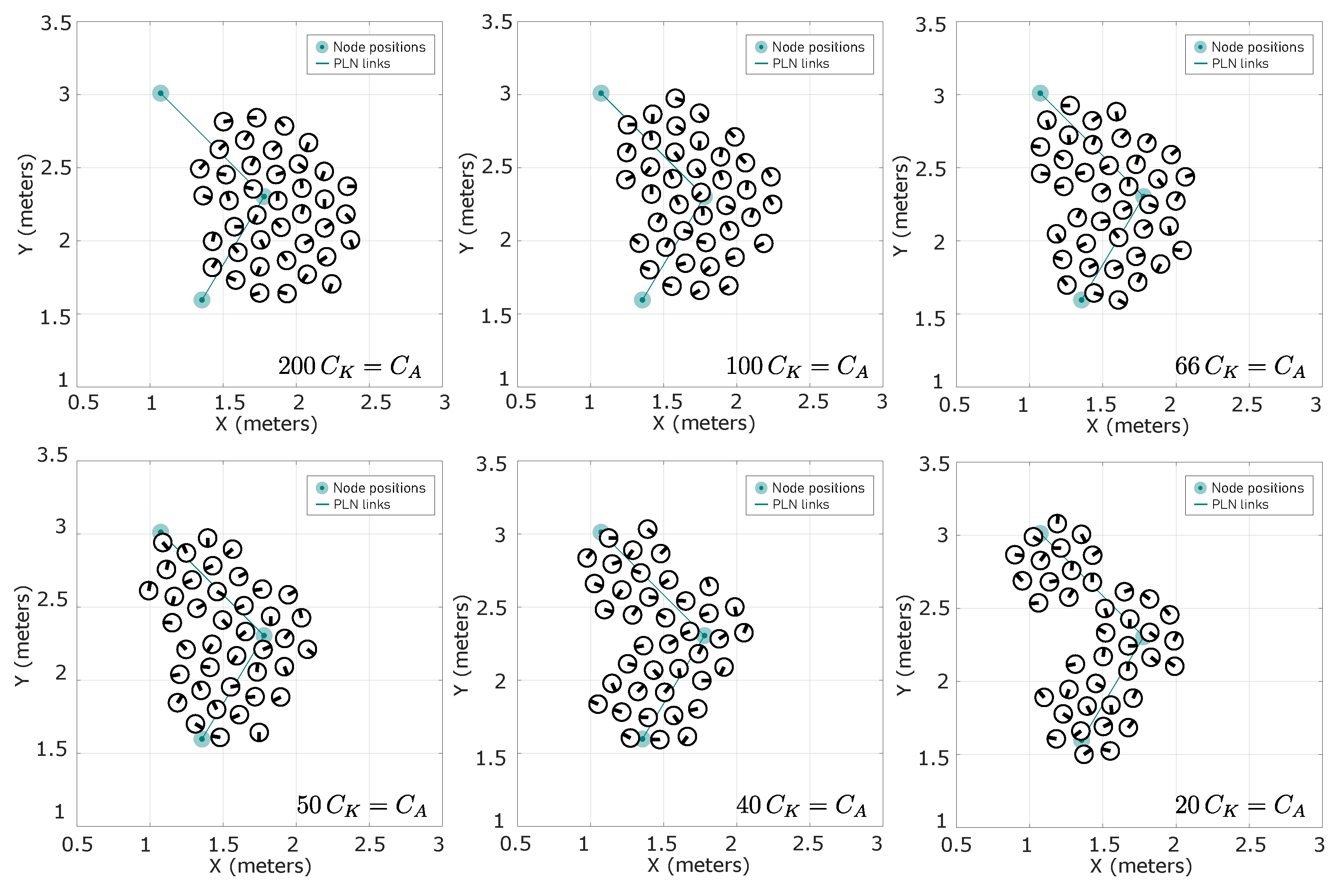
Figure 6.
Parzen-window-based density estimation and mean distance analysis.
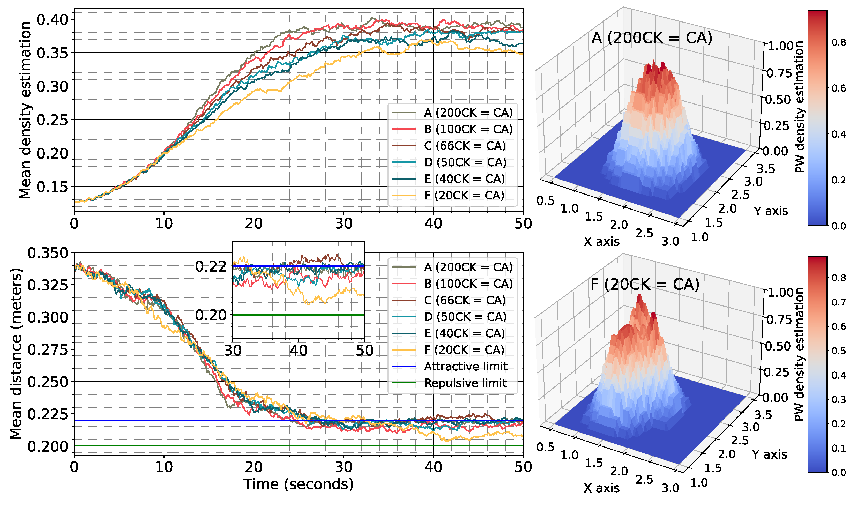
Figure 7.
Cohesive formation results for aggregation tests.
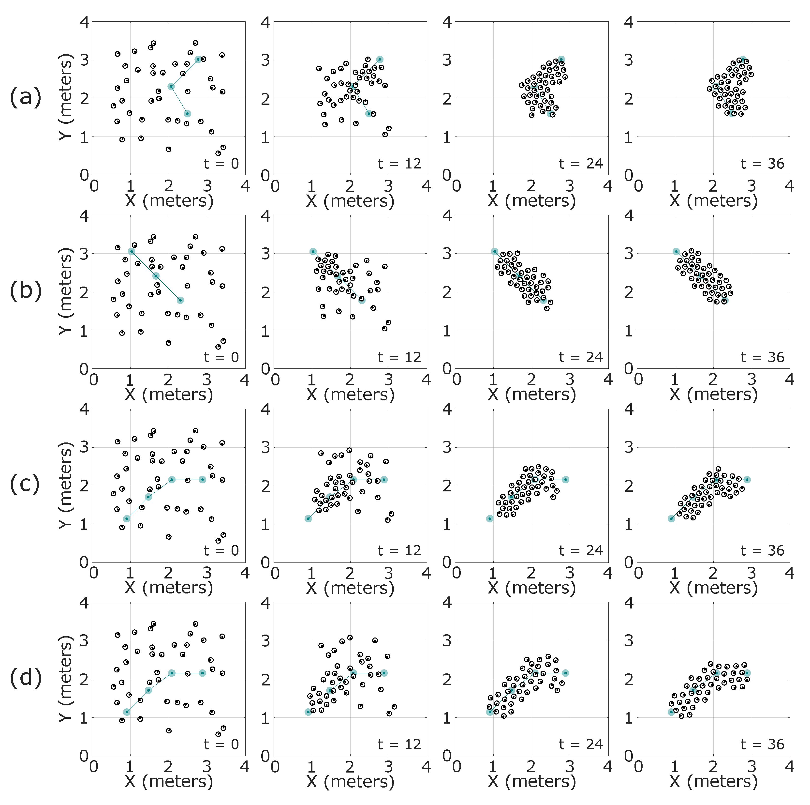
Figure 8.
Cohesion analysis for aggregation tests.
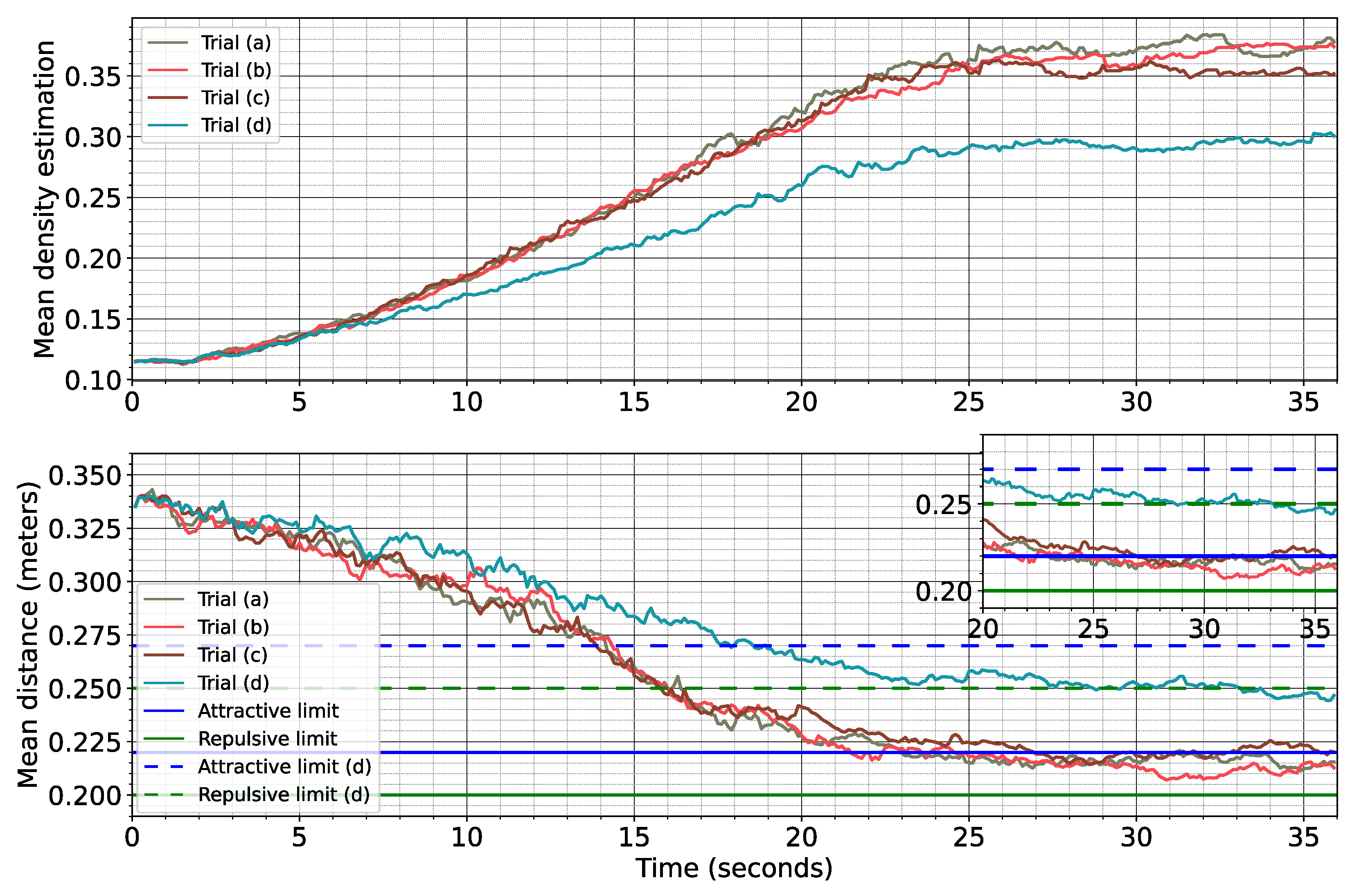
Figure 9.
Cohesive formation results for flocking tests.
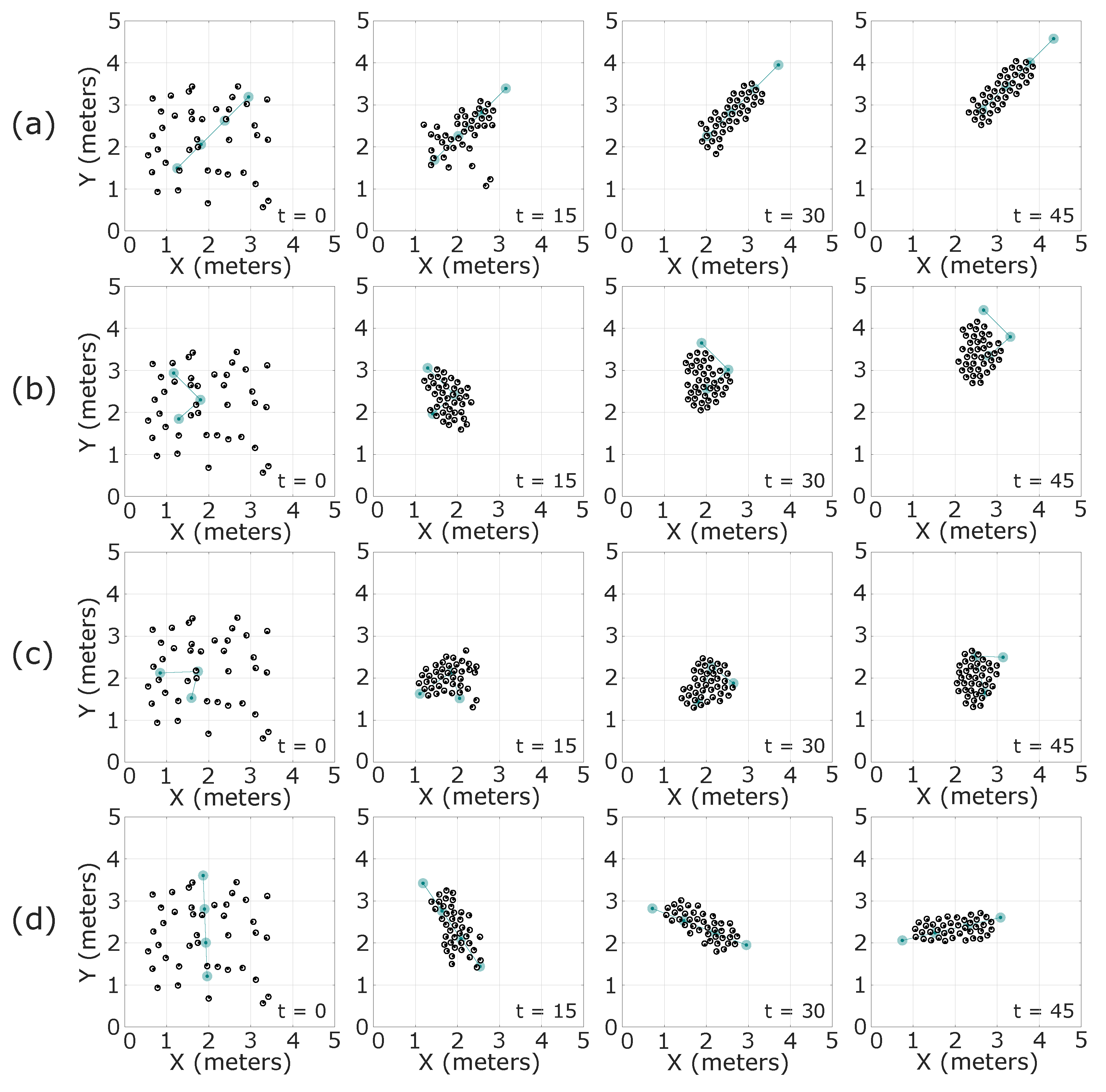
Figure 10.
Cohesion analysis for flocking tests.
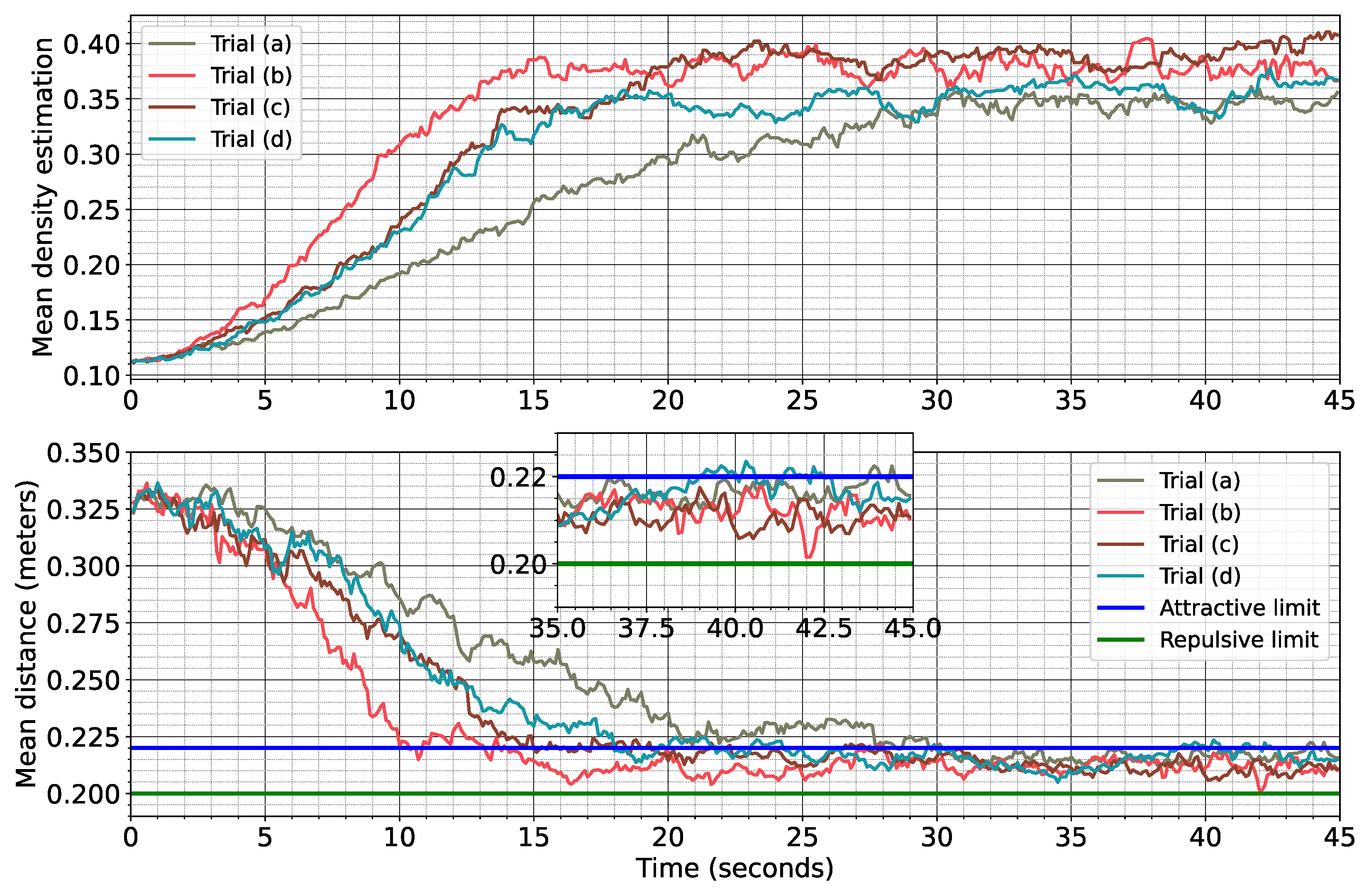
Figure 11.
Cohesive formation results for flocking tests with static obstacles.
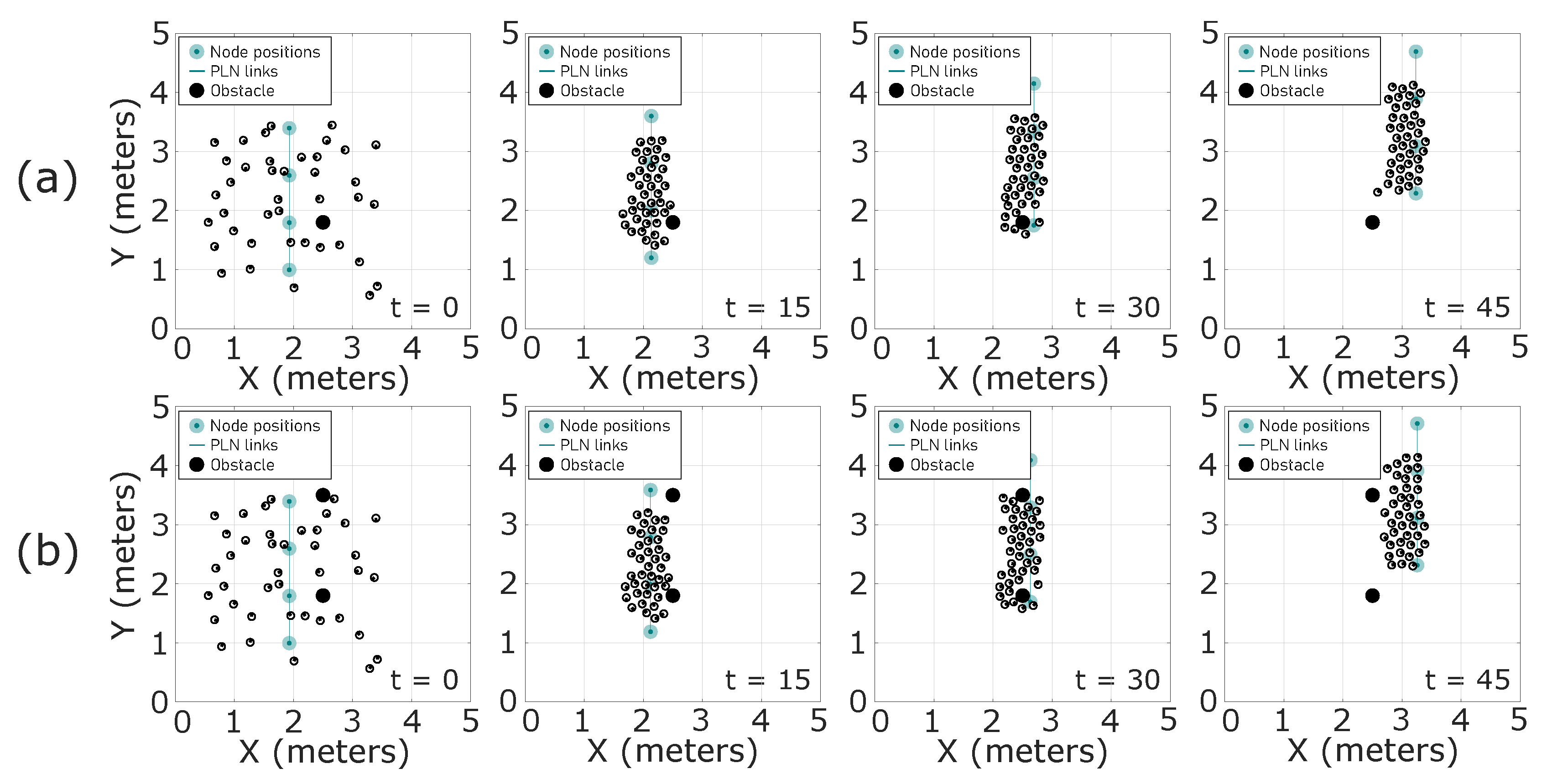
Figure 12.
Cohesive flocking formation results for large groups.
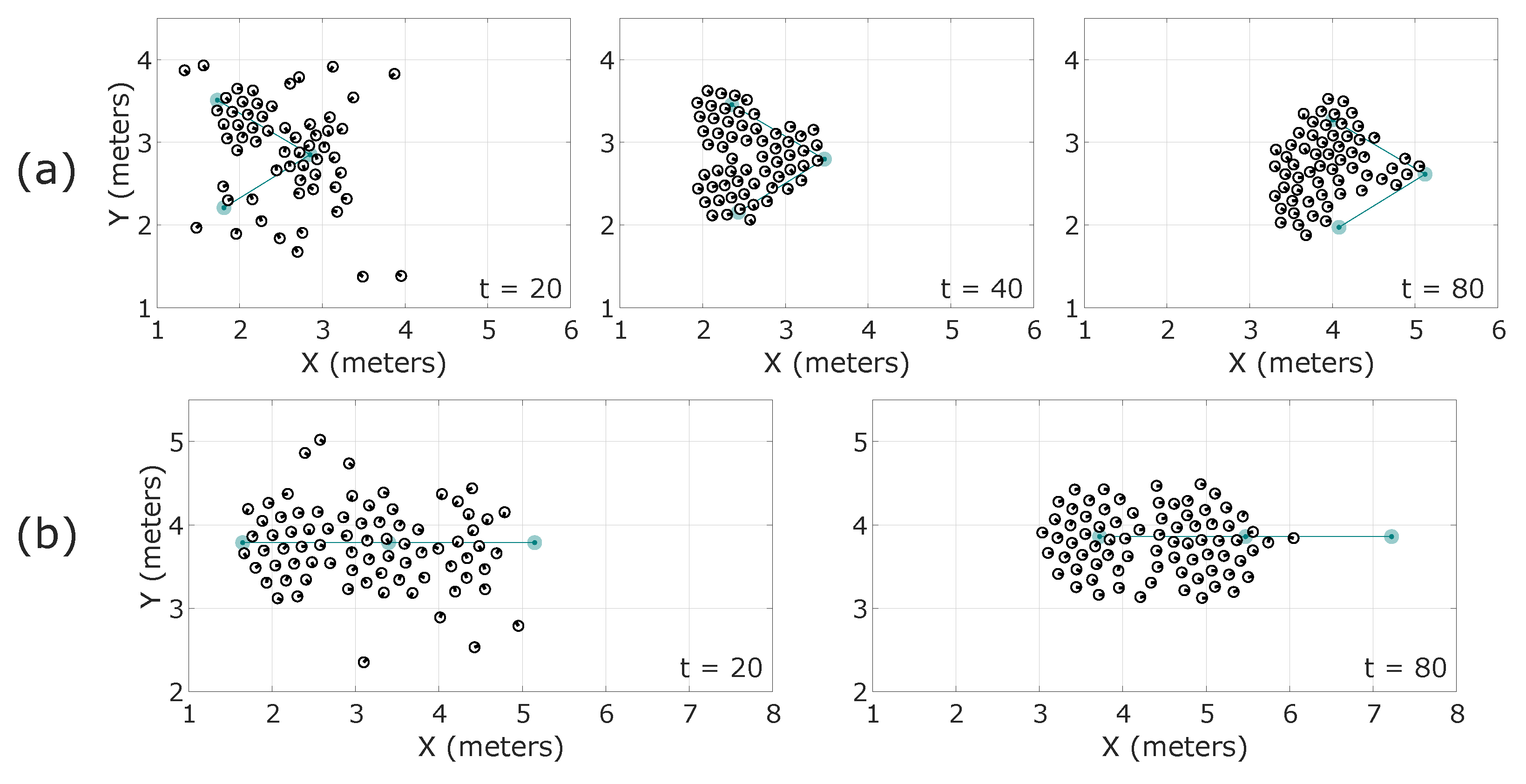
Figure 13.
Cohesion stability analysis for APFs-based gains adjustments.

Figure 14.
Linear velocity stability comparison with 10 robots for the sigmoid-based repulsive smoothing evaluation.
Figure 14.
Linear velocity stability comparison with 10 robots for the sigmoid-based repulsive smoothing evaluation.
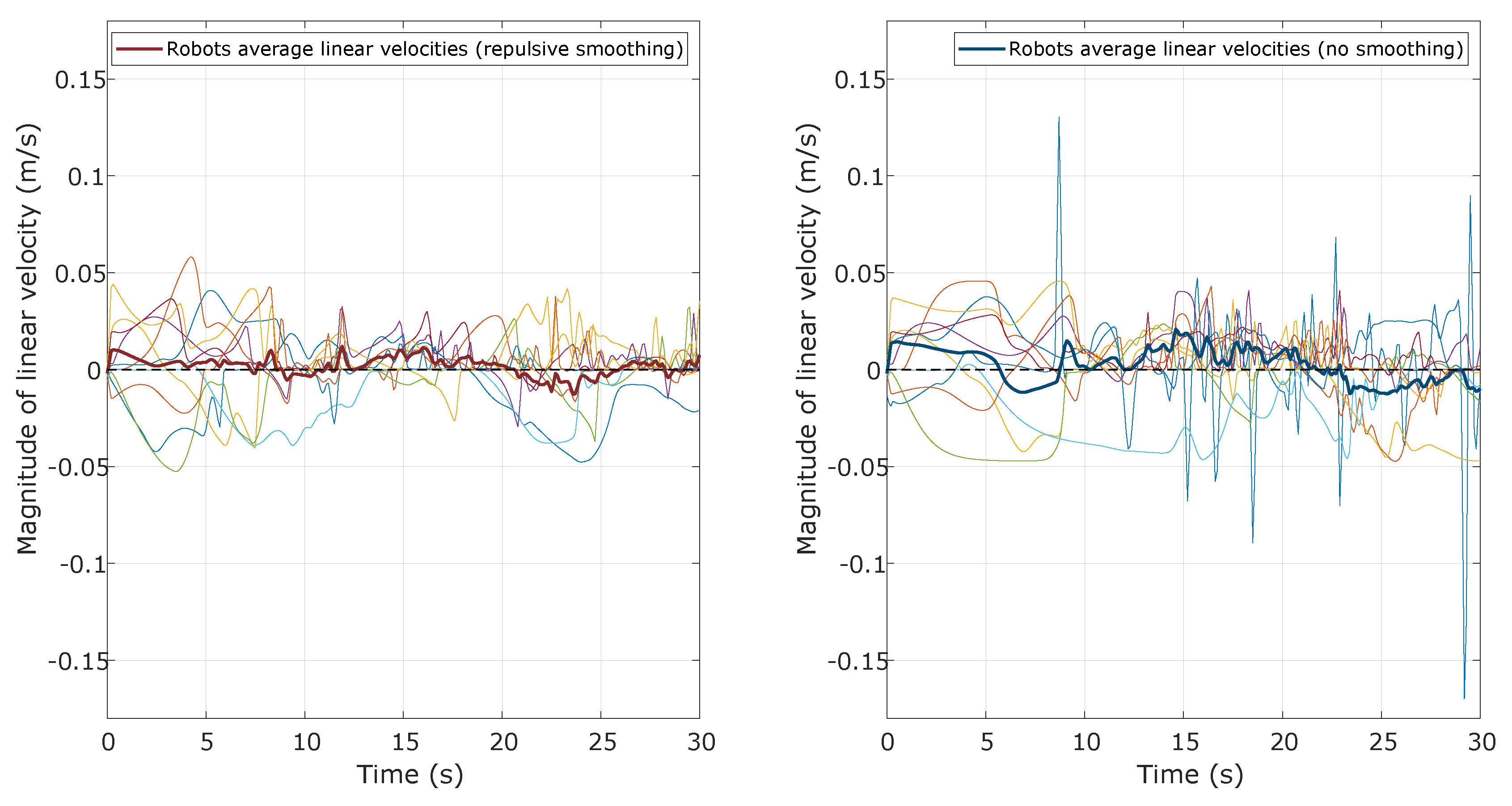
Figure 15.
Cohesive flocking formation results for a crop row environment in agriculture.
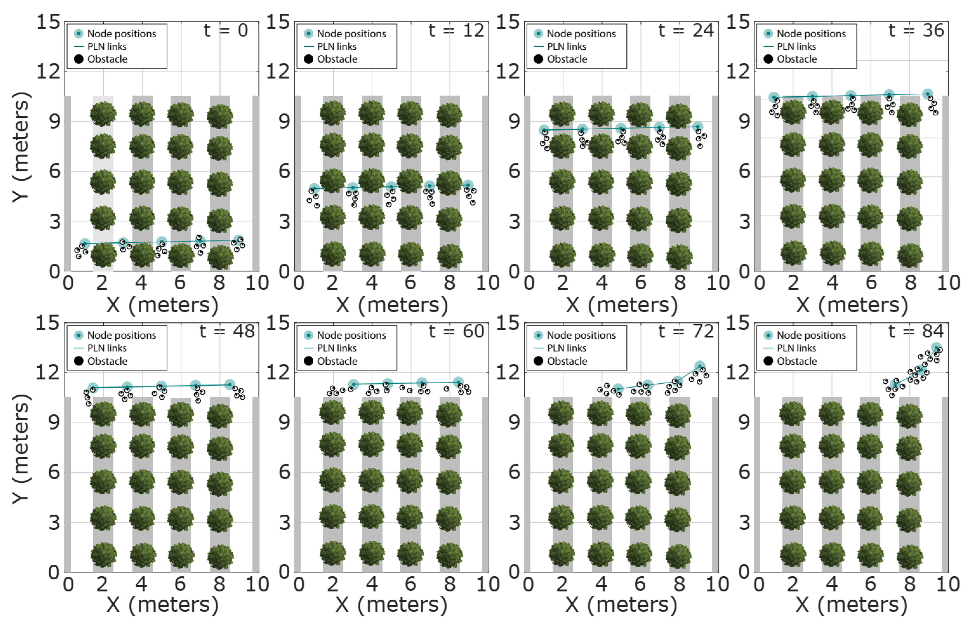
Figure 16.
Cohesive flocking motion results for a crop field in linear irregular patterns.
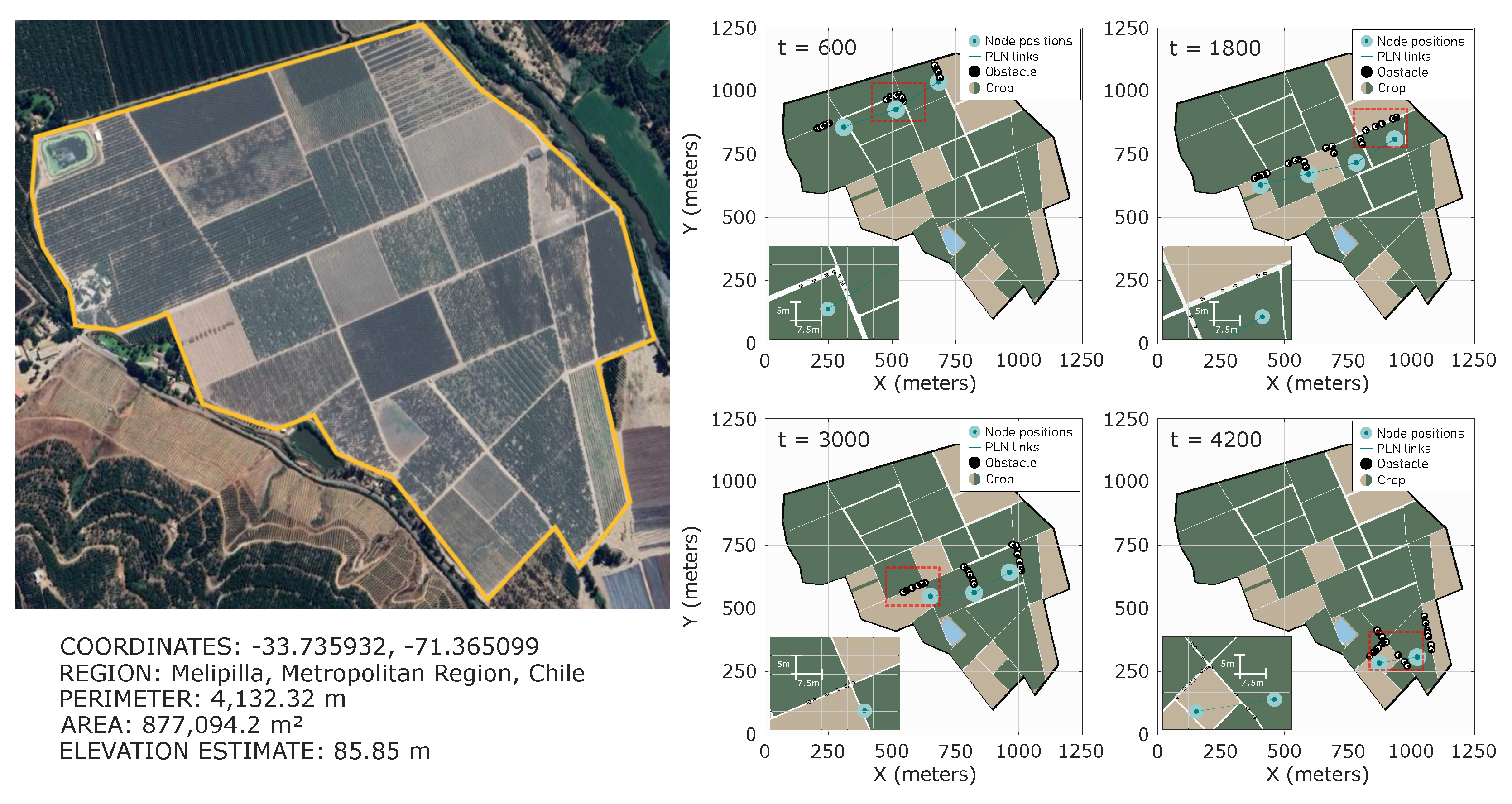
Figure 17.
Cohesive flocking motion results for a crop field with circular patterns.
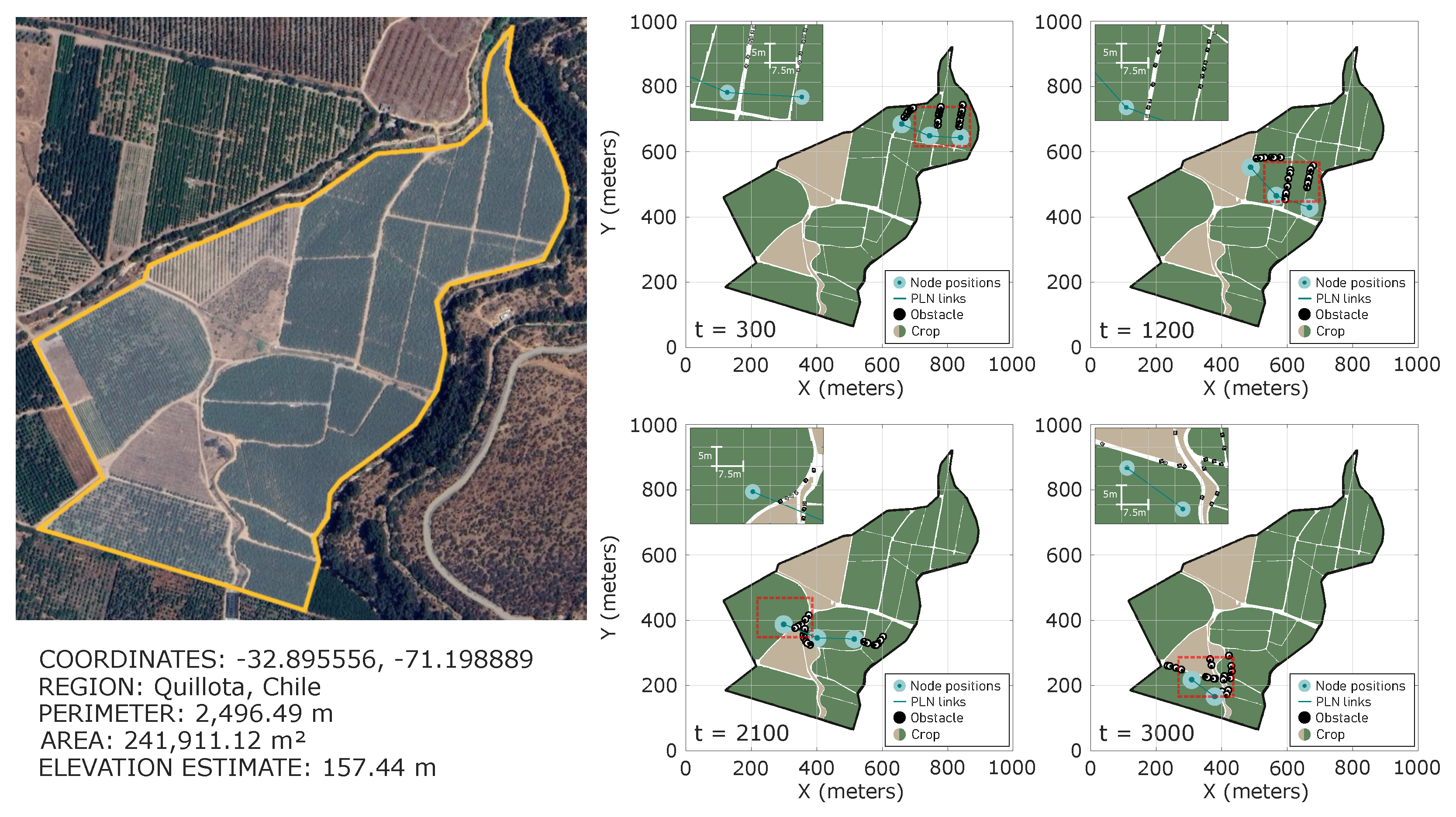
Table 2.
Simulation parameters for aggregation assessment.
| Category | Parameter | Aggregation test | |||
|---|---|---|---|---|---|
| (a) | (b) | (c) | (d) | ||
| Cohesiveness | 0.005 | 0.005 | 0.005 | 0.008 | |
| [meters] | 0.01 | 0.01 | 0.01 | 0.01 | |
| 0.2 | 0.2 | 0.2 | 0.2 | ||
| [meters] | 0.22 | 0.22 | 0.22 | 0.27 | |
| 0.01 | 0.01 | 0.01 | 0.01 | ||
| [meters] | 0.2 | 0.2 | 0.2 | 0.25 | |
| Formation | [meters] | 2 | 1.8 | 2.4 | 2.4 |
| 0.6 | 0.7 | 0.6 | 0.6 | ||
| [radians] | 0.78 | 2.35 | 3.92 | 3.92 | |
| [radians] | 4.71 | 3.14 | 2.35 | 2.35 | |
| [meters/second] | 0.0 | 0.0 | 0.0 | 0.0 | |
| [radians/second] | 0.0 | 0.0 | 0.0 | 0.0 | |
Table 3.
Simulation parameters for flocking assessment.
| Category | Parameter | Flocking test | |||
|---|---|---|---|---|---|
| (a) | (b) | (c) | (d) | ||
| Cohesiveness | 0.005 | 0.005 | 0.005 | 0.005 | |
| [meters] | 0.01 | 0.01 | 0.01 | 0.01 | |
| 0.2 | 0.2 | 0.2 | 0.2 | ||
| [meters] | 0.22 | 0.22 | 0.22 | 0.22 | |
| 0.01 | 0.01 | 0.01 | 0.01 | ||
| [meters] | 0.2 | 0.2 | 0.2 | 0.2 | |
| Formation | [meters] | 2.4 | 1.8 | 1.8 | 2.4 |
| 0.6 | 0.6 | 0.6 | 0.6 | ||
| [radians] | 0.78 | 2.35 | |||
| [radians] | 3.14 | 1.25 | 1.04 | 3.14 | |
| [meters/second] | 0.06 | 0.08 | 0.03 | 0.02 | |
| [radians/second] | 0.0 | 0.0 | 0.0005 | 0.0002 | |
Disclaimer/Publisher’s Note: The statements, opinions and data contained in all publications are solely those of the individual author(s) and contributor(s) and not of MDPI and/or the editor(s). MDPI and/or the editor(s) disclaim responsibility for any injury to people or property resulting from any ideas, methods, instructions or products referred to in the content. |
© 2025 by the authors. Licensee MDPI, Basel, Switzerland. This article is an open access article distributed under the terms and conditions of the Creative Commons Attribution (CC BY) license (http://creativecommons.org/licenses/by/4.0/).
Copyright: This open access article is published under a Creative Commons CC BY 4.0 license, which permit the free download, distribution, and reuse, provided that the author and preprint are cited in any reuse.


