Submitted:
05 December 2025
Posted:
08 December 2025
You are already at the latest version
Abstract
Fast Radio Bursts (FRBs) interactions with electrons in the ionized plasma of the intergalactic medium (IGM) produce a pulse dispersion described by classical plasma physics. The dispersion measure (DM) increases with the electron column-density, which itself is a function of the redshift–distance Hubble-Lemaître Law. This DM–redshift relation, or Macquart relation, probes the electron number-density in the IGM. The Stimulated Transfer redshift (STz) is an effect that arises from a quantum interaction of light with electrons. STz is also a function of the electron column-density but produces a photon energy loss that is observed as a redshift. Because dispersion and STz both depend on the electron column-density, a relationship between them can be expressed as a function that is independent of the column-density but proportional to a redshift cross-section constant. We find that the calculated STz cross-section agrees with the Macquart relation derived from 124 localized FRBs to better 5% accuracy. Implications on the proportion of the cosmological redshift that is due to the STz effect are discussed.
Keywords:
redshift
; fast radio bursts
; stimulated transfers
; Macquart relation
; static cosmology
1. Introduction
The Stimulated Transfer redshift (STz) is an effect that produces a new photon of reduced energy after an incoming photon is backscattered by a free electron [1]. The effect is based on the ponderomotive force, an interaction that produces a force on an electron by removing a photon from a light beam and stimulating it into another. Due to momentum-recoil, the new photon is stimulated with less energy than the original photon. A second-quantization calculation shows that the ponderomotive force has diffusive effect on electrons for multiple light beams interacting independently [2]. The electromagnetic field loses energy at a rate that produces a constant redshift , and stimulated emission ensures that no light beam suffers any angular dispersion. These properties make STz a unique effect that shares many similarities with the observed cosmological redshift without the drawbacks of its controversial variant, the tired-light redshift [3].
From the redshift per stimulated transfers and the average electron number-density in the intergalactic medium (IGM), we calculate a redshift cross-section that describes the redshift produced as radiation travels a distance through the IGM
where the redshift cross-section [2]. Solving Equation (1) yields a redshift–distance relationship with a “Hubble constant”
that is only a function of the electron number-density. Since the STz is a function of the number-density of electrons of the IGM, the total redshift over a distance is a function of the electron column-density .
From a theoretical point of view, an early semiclassical estimate of the STz cross-section yielded the value [1], and semiclassical calculation for a similar effect yielded a cross-section ,4]. It is therefore important to confirm experimentally the result of a second-quantization calculation obtained in Ref. [2], which is expected to yield an exact value of based on fundamental constants.
Using CDM determinations of the “early universe” [5] and the electron number-density1 in Equation (2), the observational route yields a cross section , a value that matches to within . Therefore, the STz effect could be large enough to almost entirely explain the cosmological redshift [2]. This justifies studying the effect in a static-Euclidean-STz framework, where the cosmological redshift is entirely due to the STz effect without any contribution from space expansion. The above comparison between and is flawed since the cosmological parameters used to calculate suffers from the missing baryon problem and the Hubble tension, producing an inaccuracy on the value of as large as . A more serious problem is that and are derived within the framework of a CDM cosmology but interpreted in a static-Euclidean-STz cosmology for the calculation of , two frameworks that are incommensurate [6] and cannot be integrated that way. To test the prediction of Equation (1) with consistency, it is therefore necessary to analyze astrophysical observations in the static-Euclidean-STz framework.
In this paper, we analyze fast radio burst (FRB) observations in the static-Euclidean-STz framework to get a value of that is independent of the electron number-density. Only since 2024 has the localization of FRBs to galactic hosts provided dispersion measures and redshift values for nearly one hundred FRBs and more. This has been of significance for cosmology [7] as these measurements have helped narrow down the value of a number of cosmological parameters [8,9,10,11,12] related to the electron column-density.
Our analysis is based on two functional relationships: the Macquart relation [13] between dispersion measure and distance, and the Hubble-Lemaître Law between distance and redshift. The dispersion measure in the static-Euclidean-STz framework is simply
where is the path length. We show that the STz effect produces a redshift that is also a function of the column density . The functional dependence of both and on the electron density allows us to eliminate from the Macquart relation and obtain a function that is only dependent on a constant [14,15].
We use a data set of 124 FRBs and analyze the DM contributions from the IGM and from the host galaxy . The latter is randomly scattered and is thought to follow a probability distribution described by a log-normal distribution [11,12,13,16], but more measurements will be necessary to confirm this distribution. To extract the Macquart relation from random host dispersion measures, we take advantage of the sharp rising edge of near . This edge-fit method mitigates the need to know the exact distribution at the expense of using a smaller subset of the FRB data with . Despite using only a fraction of all available localized FRBs, the coefficient of proportionality of the Macquart relation can be determined to a few percent accuracy. This analysis is first done in the CDM framework to confirm the reliability of the edge-fit method, and then repeated for a static-Euclidean-STz (SE-STz) framework which yields a value for .
The rest of the paper is organized as follows: Section 2 gives a derivation of the dispersion measure and the Macquart relation in the CDM and SE-STz frameworks. In Section 3 the edge-fit method is applied to obtain an observational value for in the CDM and SE-STz fameworks. The results are discussed in Section 4.
2. Dispersion Measure and the Macquart Relation
2.1. Dispersion Measure
Plasma physics predicts a frequency dispersion proportional to the electron column-density. From measurements of a delay time and frequencies of FRB signals, the observed dispersion measure (DM) is calculated as
where is the permittivity of vacuum, is the mass of an electron, e its charge, c is the speed of light in vacuum, and and are the low and high frequencies of the measured pulses separated by the delay.
The observed DM for is modeled as a sum of three different contributions
where is the contribution from the host galaxy and any gas local to the event [13], and is the contribution from the IGM to a galaxy at redshift . Both and are cosmology-model dependent contributions to the observed dispersion measure. The last term
is the Milky Way’s contribution from the interstellar medium toward and the Milky Way halo, respectively [10].
We lump the contributions from all halos, Milky Way, intersected halos in the IGM, and the halo of the host, into the constant , ignoring a possible directional and redshift dependence. A broad range of values, , have been assumed in the literature [9,10,17], and models [16,18] yield large uncertainties as their contribution is not entirely understood yet.
Since FRB events occur inside the host galaxy, and the DM is direction dependent for the Milky Way, we assume that most of the variance on comes from the host’s DM. We justify this assumption below.
The FRB data set used in this work is built from Ref. [11] augmented with the data from Refs. [9,19,20]. The resulting data set is listed in Table A1. For each two values of are given, obtained from the NE2001 [21,22] and YMW16 [23] models of the Milky Way.
For each at redshift an extragalactic DM is defined as
Both NE2001 and YMW16 are included in the analysis as separate entries, giving us a data set containing 248 entries. No FRB is excluded from this analysis.
2.2. Distribution of the Host’s Local Dispersion Measure
A log-normal distribution
is commonly used [11,12,13,16] to fit to the host DM distribution . Here, and the parameters and are adjusted to provide the best least-squares fit to the data. The log-normal distribution has a mode . We only use the mode and the coefficient of determination to characterize the spread of the distribution away from .
2.3. The Macquart Relation in Lambda-CDM Cosmology
The host contribution to in Equation (5) is given by
where the factor corrects the local to the measured value.
The IGM contribution to is the integral of the comoving electron density
where z is the redshift at distance , is the redshift at distance l, and the factor in the integrand is used for the transformation into physical coordinates [16]. is the contribution by the intergalactic medium and includes halos intersecting the line of sight [18]. The path integral excludes the high density regions near the MW and the FRB host as these are considered separately below.
The Macquart relation describes the relationship between the DM from the intergalactic medium and the redshift of the FRB’s host galaxies [18]. It can be written as[24]
where the dimensionless “Hubble-Lemaître Law” is
and is the matter density parameter. We define the Macquart constant as the proportionality factor between and ,
where is the proton mass, G is the gravitational constant, and the cosmological parameters as the Hubble constant, as the present-day baryon density parameter, and as the baryon fraction in the IGM assumed to be constant for the range of redshifts covered by the FRBs of our data set.
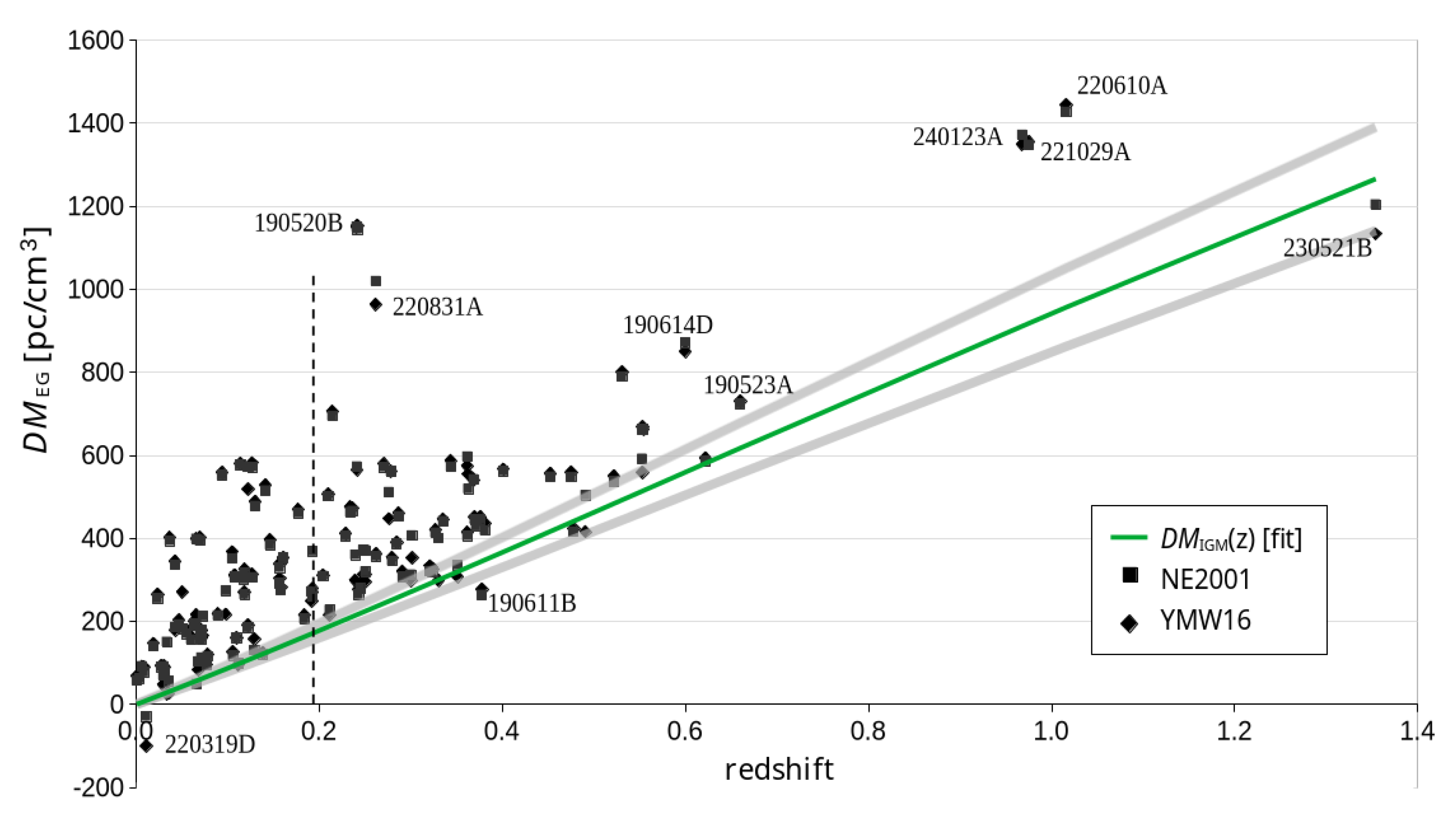
We plot the Macquart relation Equation (12) in Figure 1. The FRBs of the data set are shown with DM contribution from the Milky Way removed to obtain the extragalactic dispersion measure given by Equation (7). The green curve is calculated from a fit to 117 FRBs [10] which yielded , calculated from Equation (14) with and based on the results of Planck18 [5].
As expected, the CDM-fitted Macquart relation follows the lower edge of the scattered points where . The uncertainty of the fit, shown in gray on Figure 1, enclose most of the data points scattered around , and this for all redshifts of the data set.
A better representation of the local scatter, calculated from Equations (8) and (10), is shown in Figure 2a, where the Macquart relation has been subtracted from . Figure 2b shows the frequency distribution of the local hosts’ DM calculated with the Macquart constant . A fit to a log-normal distribution (red bars) yields a mode and a coefficient of determination , supporting the choice of the distribution in the literature [11,12,13,16].
Figure 1.
Extragalactic dispersion measure as a function of redshift for 124 FRBs and two models of Millky Way contributions to the DM. The green curve shows from Equation (12), with fitted to 117 FRBs with CDM cosmological parameters [10]. The gray curves represent the uncertainties and calculated from Ref. [10].
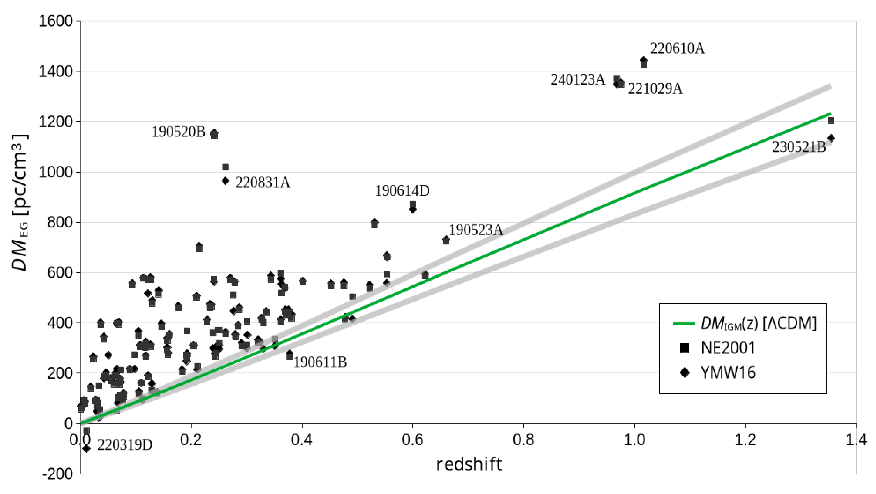
Figure 2.
(a) Local host dispersion measure as a function of redshift obtained in CDM cosmology. (b) Frequency distribution of the local host dispersion measure with binning. A fit to a log-normal distribution is shown with red bars. The negative values of are highlighted by a pink background.
Figure 2.
(a) Local host dispersion measure as a function of redshift obtained in CDM cosmology. (b) Frequency distribution of the local host dispersion measure with binning. A fit to a log-normal distribution is shown with red bars. The negative values of are highlighted by a pink background.
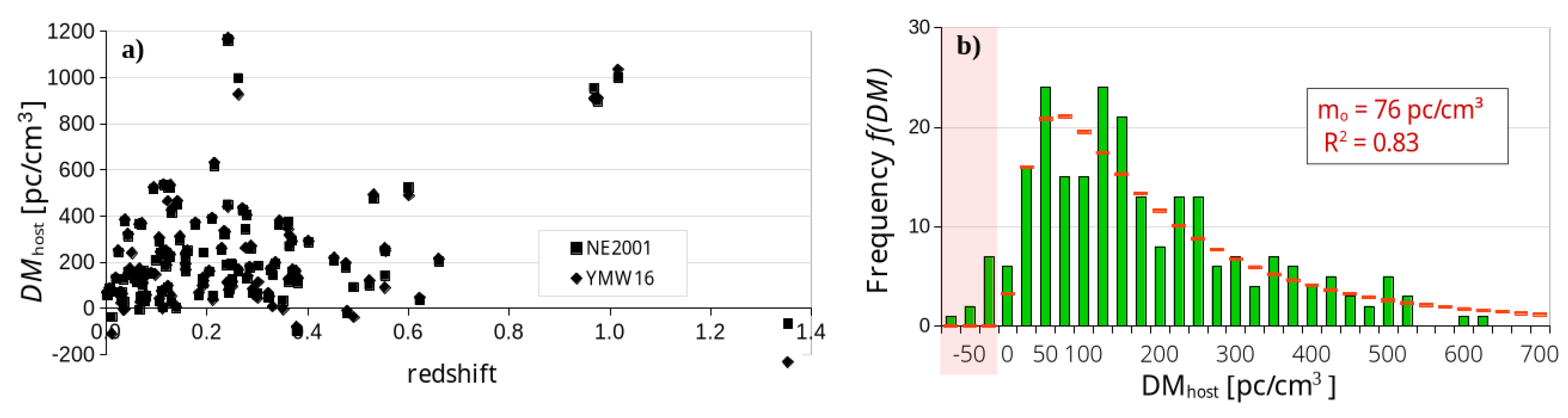
A large fraction of the data points are above , but some negative values reach a large negative DM, e.g. at , and even at . In total, fourteen hosts have a negative DM. Those are highlighted in pink in Figure 2(b). These may be due to additional contributions from overestimation by models, errors in identification of the host galaxy, and variance of the IGM density,[18] which produce some scatter that result in being negative. There could also be contributions from peculiar velocities, but even a small would correspond to a very high peculiar velocity , which is unlikely for a galaxy.
These anomalies seem to appear independently of redshift. We therefore assume that most of the variance of comes from the host’s DM, since the variance from would increase with redshift [18]. Since a negative value of is unphysical, and a positive value would only increase the number of data with an unphysical , we adopt in Equation (6) throughout this paper.
2.4. The Macquart Relation in Static-Euclidean-STz Cosmology
We derive here DM relations in the SE-STz framework mirroring the SWe derive the relations needed to
In static-Euclidean space, the host contribution to in Equation (5) is given by
The redshift–distance relationship in the SE-STz framework is derived from the rate of stimulated transfers per incident photon of wavelength is given by Equations (6)2 in Ref. [2],
where is the fine structure constant, , and is the electron number-density. Each stimulated transfer produces an energy loss that we write as the redshift increment given by Equation (7) in Ref. [2],
Multiplying Equations (16) and (17) yields a redshift rate of the entire spectrum that is independent of wavelength,[2]
This produces an energy loss first described empirically by Equations (I) of Ref. [25],
Substituting Equation (18) in Equation (19), , and , gives the redshift increase for a small propagation distance as written in Equation (1), where the redshift cross-section is
expressed only in terms of fundamental constants. The redshift cross-section represents an interaction area that produces a unit redshift.
The redshift z produced over a distance is obtained by integrating Equation (1). We note that repeated redshifts over short distance intervals combine as a product
This is a consequence of relativistic velocity-addition. Taking the logarithm allows to transform Equation (21) into a continuous summation
where we use the identity for the infinitesimal limit .
We note that the term of Equation (22) is the SE-STz equivalent of the dimensionless “Hubble-Lemaître Law” given by Equation (13) in the CDM framework, so that the SE-STz Hubble-Lemaître Law is
and hence the “Hubble constant” defined by Equation (2).
The integral term in Equation (22) is the electron column-density over the length given by Equation (3). As is the case for Equation (11), the path integral of Equation (3) excludes the high density regions near the MW and the FRB host.3 Finally, combining Equations (3) and (22) yields the Macquart relation in the SE-STz framework
where the Macquart constant
is the inverse of the STz cross-section[2] and is independent of the electron column-density[14,15].
3. Analysis
Although STz predicts a Macquart relation Equation (24) that visually fits observations, c.f. Figure 3, our goal is to obtain an uncertainty on the Macquart constant for the relation fitted to the FRB data set.
For this purpose, we use the cumulative frequency function
to determine a relative offset of the distribution. We find empirically that increases exponentially4 as a function of up to (see Figure 5), providing a position indicator of the fast-rising edge of the frequency distribution function . We use this indicator to analyze FRB data and determine
3.1. Fitting the Macquart Parameter with an Edge-Fit
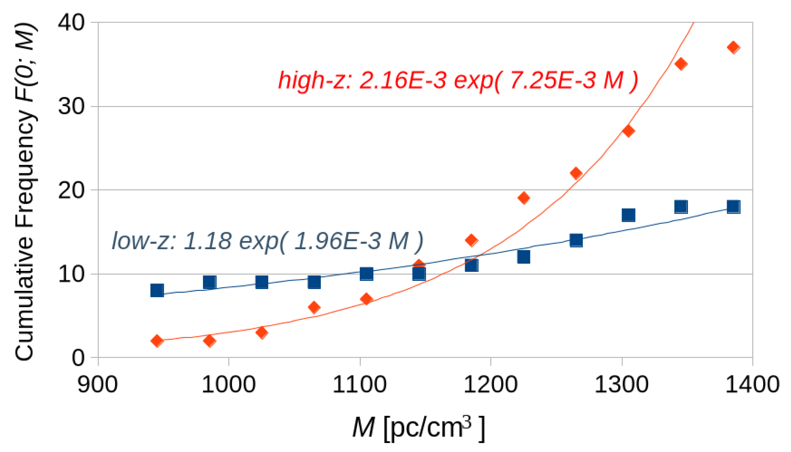
We split the FRB data set in two sets sorted by redshift, one “low-z” set containing data below the redshift median , and a “high-z” set with , where the median of our data set (Table A1) is . Figure 6 shows an example of the frequency distribution for both sub-sets, which shows good agreement between the low-z and high-z distributions. For each sub-set, the cumulative frequency function of is calculated for a Macquart constant M and evaluated at , giving the two values and .
The expected good match between the low-z and high-z distributions shows that the cumulative distributions are similar, , and independent of redshift, but only if the Macquart constant M has the correct value. An examination of Equations (11) and (24) shows that if the Macquart constant is overestimated as , will increase. From Equation (8) we find that the low-z distribution will remain almost unaffected, but the high-z distribution will shift toward low DM, which will result in . An underestimated Macquart constant will have the opposite effect such that .
It is therefore simple to find the value of M that produces an agreement between the low-z and high-z distributions by plotting and over a range of M, fitting both curves to an exponential function, and calculating the value at which they intersect. Since and depend on data near the fast rising edge of the distribution, the method is called an edge-fit.
The advantage of using the cumulative distribution in the neighbourhood of is that outliers do not ‘pull’ the fit as they would for a least-square-fit. Therefore the method does not require an arbitrary criterion that reject outliers, a criterion that could bias the final result if incorrectly selected [11]. This method also eliminates a dependence on the exact shape of the distribution and reduces a possible bias due to data points which may have been erroneously localized to an incorrect host (e.g. the actual hosts of FRB2401123A, FRB22221029A, and FRB220619A near may be at a higher redshift).
Finally, the variance on the fitted Macquart constant is estimated by using the technique of sub-sampling. Here, we randomly select 62 samples from the original 124-sample FRB data set and re-analyze the subsample as described above.5 By repeating this procedure several times, with a new random subsample each time, we can calculate an estimate of the variance of the estimator for the smaller data sets. A final estimate of from the complete data set can be calculated with .
To confirm the validity of the edge-fit analysis, we first analyze the data in the CDM framework, and then repeat the same analysis in the SE-STz framework.
3.2. Fitting the Lambda-CDM Macquart Parameter
Following the edge-fit method outlined in Section 3.1, we plot the functions and as a function of M in Figure 7. The range is limited so that does not exceed and remains within the exponential regime shown in Figure 5. The function shows a slow change as a function of M because of the proximity of the data to the origin, while the function shows a faster increase. As a result, and intersect at the value of the Macquart constant that best fits the lower edge of the scattered data in Figure 1, .
We note that the adopted does not have an effect on since both distributions are equally offset by , which does not significantly move the position of the intersection.
The evaluation uncertainty on is evaluated from sub-sampling trials as outlined in Section 3.1. The random subsamples are found to yield an average value . Since the full data set has twice the number of samples, the uncertainty on is quoted as being smaller by a factor . This yields the final estimate , or . The Macquart relation is plotted with in Figure 8, with the confidence interval shown in gray.
The edge-fit finds the value reported by Ref. [10] to within , and with an uncertainty that matches the reported uncertainty. The slightly larger uncertainty obtained from the edge-fit could be, if significant, the result of having no prior on M, while the cosmological parameters , , and were used as priors in Ref. [10]. also agrees with other determinations of the Macquart constant as well, e.g. Refs. [13,24].
This exercise demonstrates the suitability of the edge-fit method described in Section 3.1 to obtain the Macquart constant by fitting The Macquart function to the lower edge of the –z distribution of FRBs.
3.3. Fitting the STz Macquart Parameter
We repeat the edge-fit analysis in a static-Euclidean-STz (SE-STz) framework, with the Macquart relation given by Equation (24). Figure (9) shows and as a function of M. The fitted exponential functions intersect at .
Sub-sampling trials with half-size randomly selected data sets yield an average Macquart constant . We use the uncertainty on that value reduced by to estimate the uncertainty on the fit to the entire data set. This yields , or a STz cross-section
This confirms, within measurement uncertainty, the value of the fundamental redshift cross-section given by Equation (20).
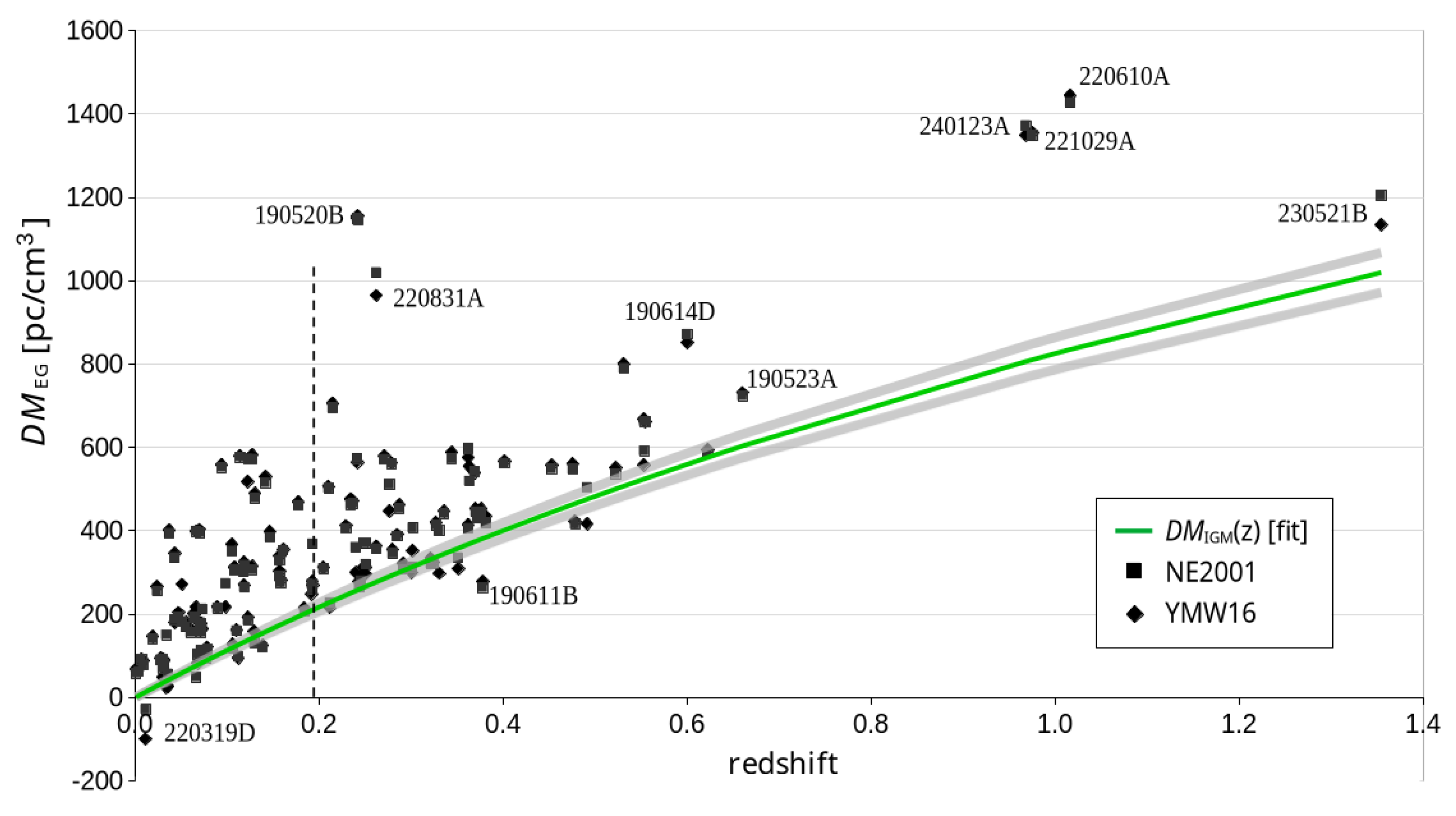
The Macquart relation with is plotted in Figure 10 with the confidence interval shown in gray. We note that the highest redshift sample FRB230521B at has a positive host DM within , a value near the median of the probability distribution function shown in Figure 4b.
Figure 9.
Functions (blue squares) and (red diamonds) as a function of . The curves show exponential fits and intersect at .
Figure 9.
Functions (blue squares) and (red diamonds) as a function of . The curves show exponential fits and intersect at .
3.4. Fitting the Halo Dispersion Measure
We have used throughout this paper. An attempt to determine was done by examining the dependence of various statistics based on a fit to a log-normal distribution. These were the mean, the median, the mode, the standard deviation of the distribution, and the coefficient of determination , for . However, no significant preference for a specific is found.
On the other hand, increasing the value of increases the number of negative , which are unphysical values. Since the edge-fit analysis is not affected by the value of , the use of has no bearing on the main results of this work.
Figure 10.
Macquart relation in the SE-STz framework for in Equation (24) (green curve), fitted to the lower edge of the –z distribution of 124 FRBs (black symbols). This yields . Gray curves: statistical confidence intervals. The vertical dashed line shows the median redshift .
Figure 10.
Macquart relation in the SE-STz framework for in Equation (24) (green curve), fitted to the lower edge of the –z distribution of 124 FRBs (black symbols). This yields . Gray curves: statistical confidence intervals. The vertical dashed line shows the median redshift .
4. Discussion
A data set containing 124 localized FRB-data provides a sufficiently large sample to fit the Macquart relation to the lower edge of the –z distribution. The edge-fit method is used in a static-Euclidean STz framework to obtain a value of the Macquart constant based on observations, and to compare this value with the cross-section of STz effect calculated from first principles.
Localized FRB dispersion measures and redshifts provide a direct measurement of . This confirms the STz cross section
to better than , independently of the value of the IGM electron number-density or any cosmological parameters. The edge-fit of the STz Macquart relation gives a slightly better fit compared to the CDM fit , indicating a good fit to observations interpreted in the SE-STz framework.
With a reliable value for , we can use the measured Hubble constant to calculate the average electron number-density in the IGM. In the SE-STz framework, only the “late” value of the Hubble constant has meaning. Substituting [26] in Equation (2) yields . We can compare this value to , with the reserve that this comparison is made across two incommensurate frameworks. These numbers may be compatible in a hybrid cosmological model of the type described in Ref. [27], but indicates that almost all cosmological redshift is caused by the STz effect. A precise measurement of the electron density number, independent of CDM’s cosmology parameters, will be needed to completely support the static-Euclidean framework.
5. Conclusions
The Stimulated Transfer redshift (STz) effect offers a promising replacement for space expansion to explain cosmological phenomena [2]. Because it is fundamentally based on stimulated emission, the effect produces a redshift without any angular dispersion of light. The interaction with electrons eliminates a frequency dependence of the resulting redshift, a property that is not possible in interactions with particles that have internal degrees of freedom. From these properties follows a redshift–distance relation , which, with the measured value of the electron number-density , closely reproduces the Hubble-Lemaître Law. The photon energy lost to electrons is observed as plasma heating in the solar corona.
Using the electron density dependence of the STz effect, we link the cosmological redshift to the dispersion observed in fast radio bursts (FRBs) through the STz cross-section . In this paper, we confirm to better than accuracy using the Macquart relation observed between dispersion measure and redshift. We show that both effects depend on known functions of the electron density through the dispersion measure, the ponderomotive force, and the Hubble-Lemaître law. Critics have argued that the STz effect fits the Hubble-Lemaître Law of cosmological redshift by coincidence. However, we demonstrate that the STz effect also quantitatively describes the Macquart relation of FRB dispersion measure. Such agreement with two very distinct phenomena – redshift and dispersion – cannot be coincidental; it confirms that STz is a common effect underlying both.
The implication of a confirmed is that the cosmological redshift is mostly produced by the STz effect, leaving very little room for space expansion and Big Bang cosmology. This explains recent observations that are difficult to reconcile with CDM, such as the presence of a mature cluster at redshift [28], a grand-design spiral galaxy at [29], and no redshift evolution of the characteristic linear sizes of galaxies [30,31]. Future research will focus on exploring the emergent properties of the Stimulated Transfer redshift, particularly regarding its implications for cosmological phenomena such as the stretching of supernova light-curves and the cosmic microwave background.
Funding
This research received no external funding.
Data Availability Statement
Acknowledgments
This research was supported by York University, which provided access to academic journals through its library. Their support is gratefully acknowledged.
Conflicts of Interest
The authors declare no conflicts of interest.
Appendix A. STz Saturation Near Bright Sources
An electron produces stimulated transfers between every beam that interacts with it. The wavefunction of every interacting light beam evolves according to the time evolution of the density matrix Equations (1) in Ref. [2]. When the wavefunction is collapsed by the transfer of a photon from one beam to another, this interrupts every other stimulated transfer in progress since the electron has received a momentum kick and is no longer coherent with the other light beams. In intergalactic space, where all interacting beams have an equal intensity, they have an equal probability of interaction with the electron.
However, the larger number of photons near a galaxy will cause rapid collapse of the wavefunction and will interrupt the slow evolution of the wavefunction during a stimulated transfer with a low intensity beam coming from large distances. As a result, a weak beam of light travelling near a bright galaxy will experience a very low rate of STz.
Even if the electron density is larger by orders of magnitudes, the brightness of the nearby galaxy is also higher by about the same amount. Quantitatively, two factors work against STz near a galaxy:
- I
- The rate of stimulated transfers cannot be greater than the rate of incoming photons from the weakest beam, and
- II
- nearby bright sources collapse the evolution of a weak beam interacting with the electron, which further reduces the STz rate for that weak beam.
As a result, electrons that produce dispersion measures and do not produce the redshift described by Equation (21) but a much smaller one by orders of magnitude. The cosmological STz is therefore only significant in the IGM, away from galaxy halos and the ISM.
Appendix B. FRB Data Set Used for this Study

| FRB | z | NE2001 | YMW16 | FRB | z | NE2001 | YMW16 | ||
|---|---|---|---|---|---|---|---|---|---|
| 200120E | 0.0008 | 87.77 | 30 | 19.54 | 181030A | 0.00385 | 103.396 | 41.1 | 33 |
| 250316A | 0.0067 | 161.82 | 70 | 70 | 171020A | 0.008672 | 114.1 | 36.7 | 24.7 |
| 220319D | 0.011228 | 110.98 | 139.7 | 211 | 231229A | 0.019 | 198.5 | 58.12 | 51.78 |
| 240210A | 0.023686 | 283.73 | 28.7 | 17.9 | 181220A | 0.02746 | 208.66 | 118.5 | 115.3 |
| 231230A | 0.0298 | 131.4 | 61.51 | 83.24 | 181223C | 0.03024 | 111.61 | 19.9 | 19.1 |
| 190425A | 0.03122 | 127.78 | 48.7 | 38.7 | 180916B | 0.0337 | 349.349 | 199 | 324.9 |
| 230718A | 0.0357 | 477 | 420.6 | 450 | 231120A | 0.0368 | 437.737 | 43.8 | 36.2 |
| 240201A | 0.042729 | 374.5 | 38.6 | 29.1 | 220207C | 0.04304 | 262.38 | 76.1 | 83.3 |
| 211127I | 0.0469 | 234.83 | 42.5 | 31.5 | 201123A | 0.0507 | 433.55 | 251.7 | 162.7 |
| 230926A | 0.0553 | 222.8 | 52.69 | 43.71 | 200223B | 0.06024 | 201.8 | 45.6 | 37 |
| 190303A | 0.064 | 223.2 | 29.8 | 21.8 | 231204A | 0.0644 | 221 | 29.73 | 21.79 |
| 231206A | 0.0659 | 457.7 | 59.13 | 59.29 | 210405I | 0.066 | 565.17 | 516.1 | 348.7 |
| 180814A | 0.068 | 190.9 | 87.6 | 107.9 | 231120A | 0.07 | 438.9 | 43.8 | 36.22 |
| 211212A | 0.0707 | 206 | 38.8 | 27.5 | 231005A | 0.0713 | 189.4 | 33.37 | 28.79 |
| 190418A | 0.07132 | 182.78 | 70.2 | 85.8 | 211212A | 0.0715 | 206 | 27.1 | 27.46 |
| 231123A | 0.0729 | 302.1 | 89.76 | 136.89 | 220912A | 0.0771 | 219.46 | 125.2 | 122.2 |
| 231011A | 0.0783 | 186.3 | 70.36 | 65.7 | 220509G | 0.0894 | 269.53 | 55.6 | 52.1 |
| 230124A | 0.0939 | 590.574 | 38.6 | 31.8 | 201124A | 0.098 | 413.52 | 139.9 | 196.6 |
| 230708A | 0.105 | 411.51 | 60.3 | 44 | 231223C | 0.1059 | 165.8 | 47.9 | 38.64 |
| 191106C | 0.10775 | 332.2 | 25 | 20.5 | 231128A | 0.1079 | 331.6 | 25.05 | 20.54 |
| 230222B | 0.11 | 187.8 | 27.7 | 26.4 | 231201A | 0.1119 | 169.4 | 70.03 | 74.72 |
| 220914A | 0.1139 | 631.28 | 54.7 | 51.1 | 190608B | 0.11778 | 338.7 | 37.3 | 26.6 |
| 230703A | 0.1184 | 291.3 | 26.97 | 20.67 | 240213A | 0.1185 | 357.4 | 40 | 32.1 |
| 203022A | 0.1223 | 706.1 | 134.13 | 188.14 | 190110C | 0.12244 | 221.6 | 37.1 | 29.9 |
| 230628A | 0.127 | 344.952 | 39 | 30.8 | 240310A | 0.127 | 601.8 | 30.1 | 19.8 |
| 210807D | 0.1293 | 251.9 | 121.2 | 93.7 | 240114A | 0.13 | 527.65 | 49.7 | 38.8 |
| 240209A | 0.1384 | 176.49 | 55.5 | 52.2 | 210410D | 0.1415 | 571.2 | 56.2 | 42.2 |
| 230203A | 0.1464 | 420.1 | 36.29 | 22.98 | 231226A | 0.1569 | 329.9 | 38.1 | 26.7 |
| 230526A | 0.157 | 361.4 | 31.9 | 21.9 | 220920A | 0.158239 | 314.99 | 39.9 | 33.4 |
| 200430A | 0.1608 | 380.1 | 27.2 | 26.1 | 210603A | 0.1772 | 500.147 | 39.5 | 30.8 |
| 220529A | 0.1839 | 246 | 40 | 30.9 | 230311A | 0.1918 | 364.3 | 92.39 | 115.68 |
| 220725A | 0.1926 | 290.4 | 30.7 | 11.6 | 121102A | 0.19273 | 557 | 188.4 | 287.1 |
| 221106A | 0.2044 | 343.8 | 34.8 | 31.8 | 240215A | 0.21 | 549.5 | 47.9 | 42.8 |
| 230730A | 0.2115 | 312.5 | 85.18 | 97.29 | 210117A | 0.2145 | 729.1 | 34.4 | 23.1 |
| 221027A | 0.229 | 452.5 | 47.2 | 40.59 | 191001A | 0.234 | 506.92 | 44.2 | 31.1 |
| 190714A | 0.2365 | 504.13 | 38.5 | 31.2 | 221101B | 0.2395 | 491.554 | 131.2 | 192.4 |
| 190520B | 0.241 | 1210.3 | 60.1 | 60.1 | 220825A | 0.241397 | 651.24 | 78.5 | 86.9 |
| 190520B | 0.2418 | 1204.7 | 60.2 | 50.2 | 191228A | 0.2432 | 297.5 | 32.9 | 20.1 |
| 231017A | 0.245 | 344.2 | 64.55 | 55.64 | 220307B | 0.248123 | 499.27 | 128.2 | 186.9 |
| 221113A | 0.2505 | 411.027 | 91.7 | 115.4 | 220307B | 0.2507 | 499.15 | 128.2 | 186.98 |
| 220831A | 0.262 | 1146.25 | 126.8 | 182.3 | 231123B | 0.2621 | 396.857 | 40.3 | 33.8 |
| 230307A | 0.2706 | 608.854 | 37.6 | 29.5 | 221116A | 0.2764 | 643.448 | 132.3 | 196.2 |
| 220105A | 0.2785 | 583 | 22 | 20.6 | 210320C | 0.2797 | 384.8 | 39.3 | 30.4 |
| 221012A | 0.284669 | 441.08 | 54.3 | 50.5 | 240229A | 0.287 | 491.15 | 38 | 29.5 |
| 190102C | 0.2912 | 364.5 | 57.4 | 43.3 | 220506D | 0.30039 | 396.97 | 84.6 | 97.7 |
| 230501A | 0.3015 | 532.471 | 125.7 | 180.2 | 180924B | 0.3212 | 361.42 | 40.5 | 27.6 |
| 231025B | 0.3238 | 368.7 | 48.67 | 43.36 | 230626A | 0.327 | 452.723 | 39.3 | 32.5 |
| 180301A | 0.3304 | 552 | 151.7 | 254 | 231220A | 0.3355 | 491.2 | 49.9 | 44.5 |
| 211203C | 0.3439 | 636.2 | 63.7 | 48.4 | 220208A | 0.351 | 437 | 101.6 | 128.8 |
| 220726A | 0.3619 | 686.232 | 89.5 | 111.4 | 230902A | 0.3619 | 440.1 | 34.1 | 25.5 |
| 220717A | 0.36295 | 637.34 | 118.3 | 83.2 | 200906A | 0.3688 | 577.8 | 35.8 | 37.9 |
| 240119A | 0.37 | 483.1 | 37.9 | 30.98 | 220330D | 0.3714 | 468.1 | 38.6 | 30.09 |
| 240119A | 0.376 | 483.1 | 38 | 31 | 190611B | 0.3778 | 321.4 | 57.8 | 43.7 |
| 220501C | 0.381 | 449.5 | 30.6 | 14 | 220204A | 0.4012 | 612.584 | 50.7 | 46 |
| 230712A | 0.4525 | 587.567 | 39.2 | 30.9 | 181112A | 0.4755 | 589.27 | 41.7 | 29 |
| 220310F | 0.477958 | 462.24 | 46.3 | 39.5 | 220918A | 0.491 | 656.8 | 153.1 | 240.6 |
| 190711A | 0.522 | 593.1 | 56.5 | 42.6 | 230216A | 0.531 | 828 | 38.5 | 27.05 |
| 221219A | 0.553 | 706.708 | 44.4 | 38.6 | 230814A | 0.553 | 696.4 | 104.8 | 137.8 |
| 221219A | 0.554 | 706.7 | 44.4 | 44.4 | 190614D | 0.6 | 959.2 | 87.8 | 108.7 |
| 220418A | 0.622 | 623.25 | 36.7 | 29.5 | 190523A | 0.66 | 760.8 | 37.2 | 29.9 |
| 240123A | 0.968 | 1462 | 90.2 | 113 | 221029A | 0.975 | 1391.75 | 43.8 | 36.4 |
| 220610A | 1.016 | 1458.15 | 31 | 13.6 | 230521B | 1.354 | 1342.9 | 138.8 | 209.7 |
References
- Marmet, L. Optical Forces as a Redshift Mechanism: the “Spectral Transfer Redshift”. In Proceedings of the 2nd Crisis in Cosmology Conference, CCC-2; Potter, F., Ed., San Francisco, CA, May 2009; Vol. 413, ASP Conference Series, pp. 268–276. http://aspbooks.org.
- Marmet, L. Diffusive interactions between photons and electrons: an application to cosmology. In Proceedings of the 17th Marcel Grossmann Meeting; Ruffini, R.; Vereshchagin, G., Eds. World Scientific Publishing Company, 2024. Preprint arXiv:2410.02036.
- López-Corredoira, M.; Marmet, L. Alternative ideas in cosmology. Int. J. Mod. Phys. D 2022, 31, 2230014–1–37. arXiv:2202.12897. [CrossRef]
- Ashmore, L. Recoil Between Photons and Electrons Leading to the Hubble Constant and CMB. Galilean Electrodyn. 2006, 17, 53–57.
- Aghanim, N.; Akrami, Y.; Ashdown, M.; et al.. Planck 2018 results - VI. Cosmological parameters. A&A 2020, 641, A6. [CrossRef]
- Kuhn, T. The structure of scientific revolutions; Number 2 in International encyclopedia of unified science. Foundations of the unity of science Vol. 2, University of Chicago Press, 1970; pp. i–210. 2nd Ed., Enl. ISBN 9780226458144.
- Lorimer, D.; McLaughlin, M.; Bailes, M. The discovery and significance of fast radio bursts. Astrophys Space Sci 2024, 369, 59. [CrossRef]
- Jia, J.Y.; Qiang, D.C.; Li, L.Y.; Wei, H. Generalized Distributions of Host Dispersion Measures in the Fast Radio Burst Cosmology. arXiv 2025. [CrossRef]
- Acharya, S.; Beniamini, P. Utilizing localized fast radio bursts to constrain their progenitors and the expansion history of the Universe. J. Cosmol. Astropart. Phys. 2025, 981, 73–97. [CrossRef]
- Zhuge, J.; Kalomenopoulos, M.; Zhang, B. Hubble constant constraint using 117 FRBs with a more accurate probability density function for DMdiff. arXiv 2025. Accepted for publication in ApJ., . [CrossRef]
- Wang, Y.Y.; Gao, S.J.; Fan, Y.Z. Probing Cosmology with 92 Localized Fast Radio Bursts and DESI BAO. Apj 2025, 981, 9–18. [CrossRef]
- Piratova-Moreno, E.; García, L.; Benavides-Gallego, C.; Cabrera, C. Fast Radio Bursts as cosmological proxies: estimating the Hubble constant. arXiv 2025. [CrossRef]
- Macquart, J.P.; Prochaska, J.; McQuinn, M.; Bannister, K.; Bhandari, S.; Day, C.; Deller, A.; Ekers, R.; James, C.; Marnoch, L.; et al. A census of baryons in the Universe from localized fast radio bursts. Nature 2020, 581, 391–395. [CrossRef]
- Ashmore, L. A Relationship between Dispersion Measure and Redshift Derived in Terms of New Tired Light. JHEPGC 2016, 2, 512–530. [CrossRef]
- Marmet, L. Source of a Fast Radio Burst identified: implications for some tired-light redshift theories. hal-04772264, 2017. hal.science/hal-04772264v1.
- Reischke, R.; Kovač, M.; Nicola, A.; Hagstotz, S.; Schneider, A. An analytical model for the dispersion measure of Fast Radio Burst host galaxies. The Open Journal of Astrophysics 2025, 8. [CrossRef]
- Kalita, S.; Bhatporia, S.; Weltman, A. Fast Radio Bursts as probes of the late-time universe: a new insight on the Hubble tension. Physics of the Dark Universe 2025, 48, 101926. [CrossRef]
- Baptista, J.; Prochaska, J.; Mannings, A.; James, C.; Shannon, R.; Ryder, S.; Deller, A.; Scott, D.; Glowacki, M.; Tejos, N. Measuring the Variance of the Macquart Relation in Redshift–Extragalactic Dispersion Measure Modeling. ApJ 2024, 965, 57–67. [CrossRef]
- Connor, L.; Ravi, V.; Sharma, K.; Ocker, S.K.; Faber, J.; Hallinan, G.; Harnach, C.; Hellbourg, G.; Hobbs, R.; Hodge, D.; et al. A gas-rich cosmic web revealed by the partitioning of the missing baryons. Nat Astron 2025, pp. 1–14. [CrossRef]
- The CHIME/FRB Collaboration: et al. FRB 20250316A: A Brilliant and Nearby One-off Fast Radio Burst Localized to 13 pc Precision. ApJL 2025, 989, L48. [CrossRef]
- Cordes, J.; Lazio, T. NE2001.I. A New Model for the Galactic Distribution of Free Electrons and its Fluctuations. arXiv 2002. [CrossRef]
- Cordes, J.; Lazio, T. NE2001. II. Using Radio Propagation Data to Construct a Model for the Galactic Distribution of Free Electrons. arXiv 2003. [CrossRef]
- Yao, J.; Manchester, R.; Wang, N. A New Electron-Density Model for Estimation of Pulsar and FRB Distances. ApJ 2017, 835, 32. [CrossRef]
- Wang, B.; Wei, J.J.; Wu, X.F.; López-Corredoira, M. Revisiting constraints on the photon rest mass with cosmological fast radio bursts. J. Cosmol. Astropart. Phys. 2023, 2023, 25. [CrossRef]
- Nernst, W. Weitere Prüfung der Annahme eines stationären Zustandes im Weltall. Z. Phys. 1937, 106, 633–661. A translation is available in Aperion 2(3) July 1995, http://redshift.vif.com/JournalFiles/Pre2001/V02NO3PDF/V02N3NER.PDF.
- Riess, A.G.; Li, S.; Anand, G.; Yuan, W.; Breuval, L.; Casertano, S.; Macri, L.M.; Scolnic, D.; Murakami, Y.S.; Filippenko, A.V.; et al. The Perfect Host: JWST Cepheid Observations in a Background-Free SN Ia Host Confirm No Bias in Hubble-Constant Measurements. arXiv 2025. [CrossRef]
- Gupta, R. Static and Dynamic Components of the Redshift. International Journal of Astronomy and Astrophysics 2018, 8, 219–229. Art. no. 3, . [CrossRef]
- Witten, C.; Oesch, P.A.; McClymont, W.; Meyer, R.A.; Fudamoto, Y.; Sijacki, D.; Laporte, N.; Bennett, J.S.; Simmonds, C.; Giovinazzo, E.; et al. Before its time: a remarkably evolved protocluster core at z=7.88. arXiv 2025. Submitted to A&A, . [CrossRef]
- Jain, R.; Wadadekar, Y. A grand-design spiral galaxy 1.5 billion years after the Big Bang with JWST. A&A 2025, 703, A96. [CrossRef]
- Lovyagin, N.; Raikov, A.; Yershov, V.; Lovyagin, Y. Cosmological Model Tests with JWST. Galaxies 2022, 10, 108–127. [CrossRef]
- Raikov, A.; Tsymbal, V.; Lovyagin, N. Cosmological observational tests in the JWST Era I: angular size - redshift. arXiv 2025. [CrossRef]
| 1 | |
| 2 | The phase factor given by Equations (6) in Ref. [2] can be shown to be exactly . |
| 3 | Despite an electron number-density larger by several orders of magnitude near and , stimulated transfers are saturated by the large luminosity of the nearby galaxy and produce little additional redshift. As a result of this saturation, stimulated transfers near a galaxy occur at essentially the same rate as they do in the IGM and contribute to a negligible redshift over the size of a galaxy. A more detailed explanation is given in Appendix A. |
| 4 | Interestingly, an exponential onset of the cumulative distribution-function is a characteristic of the maximum Gumbel distribution, which is similar to the observed distribution. |
| 5 |
and are selected independently for each FRB, giving subsamples consisting of 124 random samples from 248 pairs. |
Figure 3.
STz Macquart relation for 124 FRBs. The blue line shows the STz Macquart relation as given by Equation (24), where the Macquart constant is exactly . The relation follows the lower edge of the –z distribution of 124 FRBs (black symbols) where .
Figure 3.
STz Macquart relation for 124 FRBs. The blue line shows the STz Macquart relation as given by Equation (24), where the Macquart constant is exactly . The relation follows the lower edge of the –z distribution of 124 FRBs (black symbols) where .
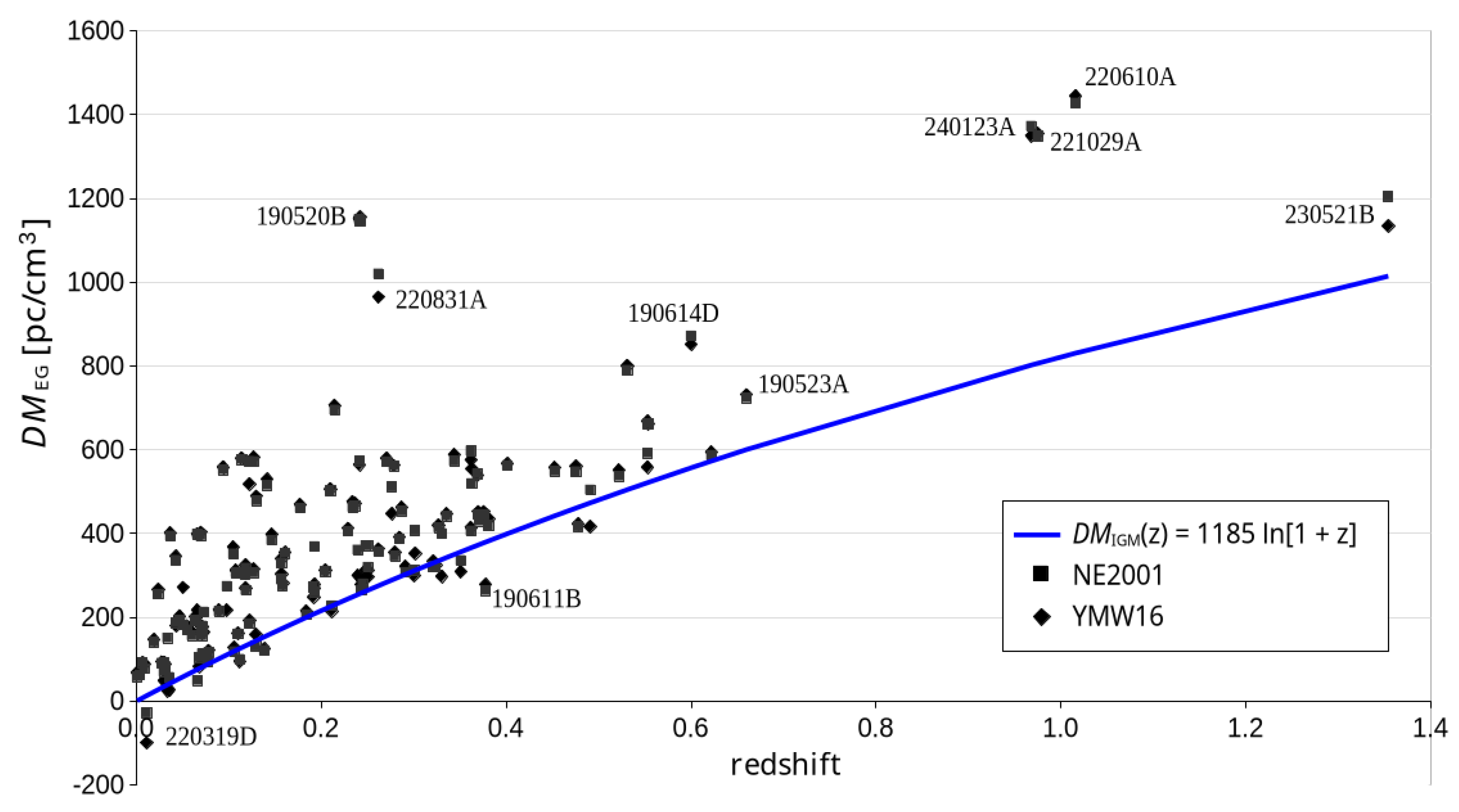
Figure 4.
(a) Host dispersion measure as a function of redshift obtained in the SE-STz framework. (b) Frequency distribution of the local host dispersion measure plotted shown with binning. A fit to a log-normal distribution (red bars) has a mode and a coefficient of determination . The negative values of are highlighted by a pink background.
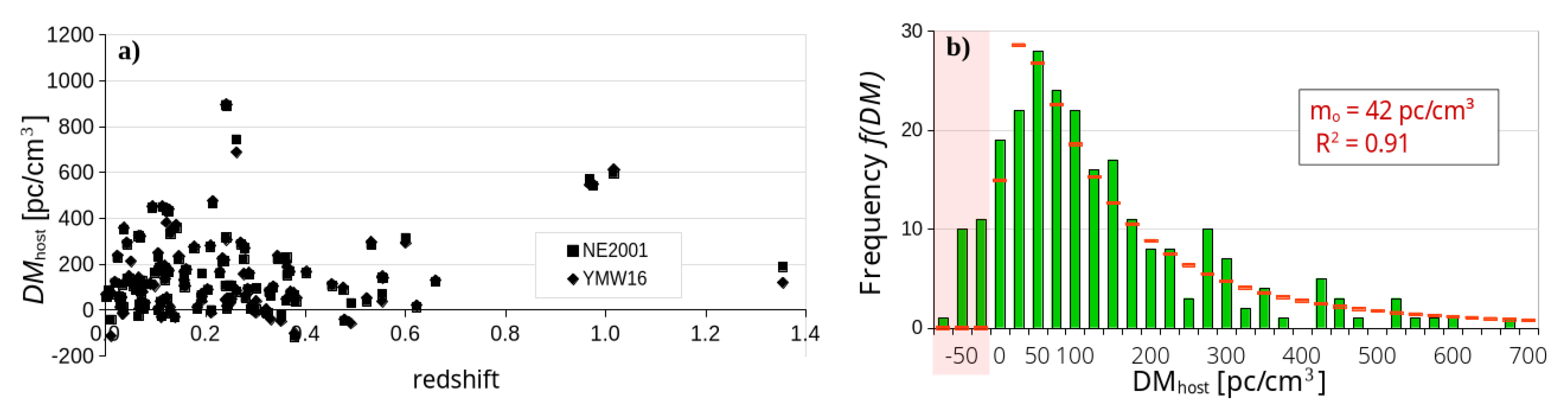
Figure 5.
Cumulative distribution of from Figure 2(b) in the CDM framework (black curve). increases exponentially up to , as shown by the red curve.
Figure 5.
Cumulative distribution of from Figure 2(b) in the CDM framework (black curve). increases exponentially up to , as shown by the red curve.
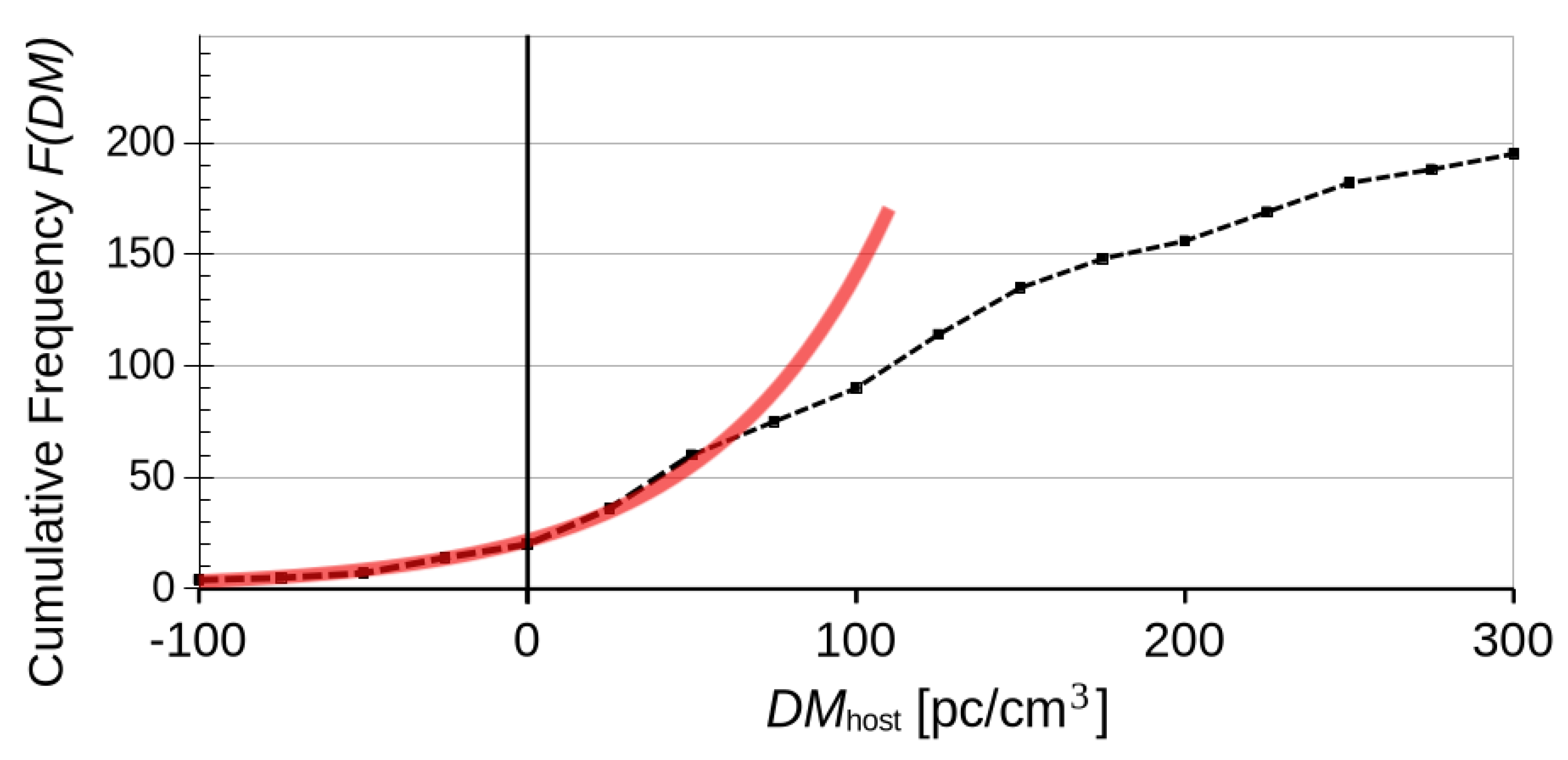
Figure 6.
Distribution of dm-host for the low-z sub-set (in yellow) and the high-z sub-set (in red) for and the Macquart relation Equation (24). The distributions have been smoothed with a Gaussian filter to improve the visualization.
Figure 6.
Distribution of dm-host for the low-z sub-set (in yellow) and the high-z sub-set (in red) for and the Macquart relation Equation (24). The distributions have been smoothed with a Gaussian filter to improve the visualization.
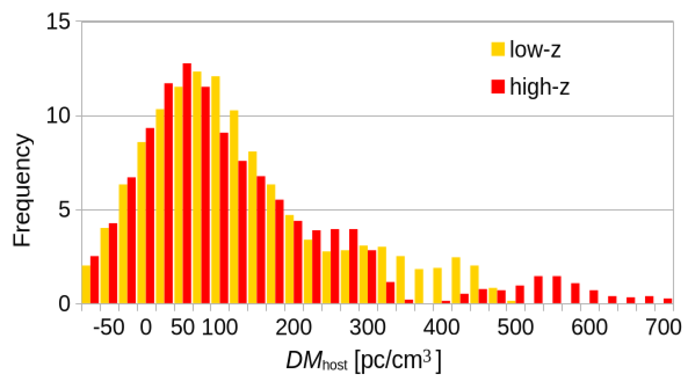
Figure 7.
Functions (blue squares) and (red diamonds) as a function of . The curves show exponential fits and intersect at .
Figure 7.
Functions (blue squares) and (red diamonds) as a function of . The curves show exponential fits and intersect at .
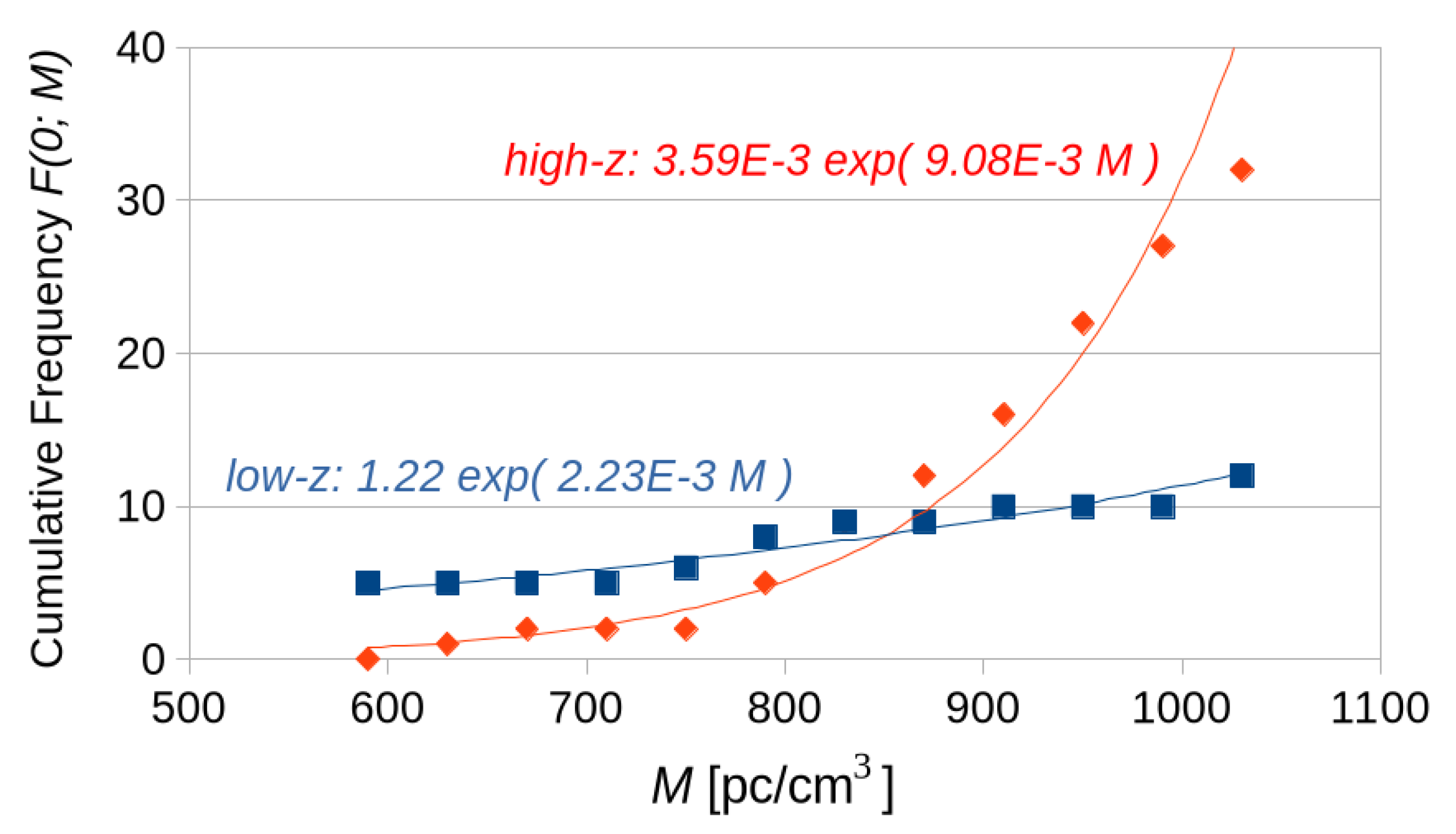
Figure 8.
Macquart relation for given by Equation (12) (green curve), fitted to the lower edge of the –z distribution of 124 FRBs (black symbols), yields . Gray curves: statistical confidence intervals. The vertical dashed line shows the median redshift . This figure shows that the edge-fit gives a Macquart constant that is essentially equivalent to the CDM-fit shown in Figure 1.
Disclaimer/Publisher’s Note: The statements, opinions and data contained in all publications are solely those of the individual author(s) and contributor(s) and not of MDPI and/or the editor(s). MDPI and/or the editor(s) disclaim responsibility for any injury to people or property resulting from any ideas, methods, instructions or products referred to in the content. |
© 2025 by the authors. Licensee MDPI, Basel, Switzerland. This article is an open access article distributed under the terms and conditions of the Creative Commons Attribution (CC BY) license (http://creativecommons.org/licenses/by/4.0/).
Copyright: This open access article is published under a Creative Commons CC BY 4.0 license, which permit the free download, distribution, and reuse, provided that the author and preprint are cited in any reuse.


