
Submitted:
05 December 2025
Posted:
05 December 2025
You are already at the latest version
Abstract
The structural vibration of industrial droplet dispensers can be modeled by telegraph-like equations to a good approximation. We reinterpret the telegraph equation from the standpoint of an electric-circuit system consisting of an inductor and a resistor, which is in interaction with an environment, say, a substrate. This interaction takes place through a capacitor and a shunt resistor. Such interactions serve as leakage. We have performed analytical investigation of the frequency dispersion of telegraph equations over unbounded one-dimensional domain. By varying newly identified key parameters, we have not only recovered the well-known characteristics but also discovered crossover phenomena regarding phase and group velocities. We have examined frequency responses of the electric circuit underlying telegraph equations, thereby confirming the role as low-pass filters. By identifying a set of physically meaningful reduced cases, we have laid foundations on which we could further explore wave propagations over finite domain with appropriate side conditions.
Keywords:
telegraph equation
; string vibration
; droplet dispenser
; system-environment interaction
; frequency dispersion
; phase velocity
; group velocity
; response function
1. Introduction
As a partial differential equation (PDE) [1,2], the telegraph equation is used as a model for the dynamics of electric potential and electric current on a lossy transmission line [3,4,5]. From broader perspectives, telegraph-like equations describe diverse phenomena in nature, biology, and industrial devices, for instance: [i] dispersion in turbulent flows [6], [ii] flows through hollow tubes [7,8], [iii] structural dynamics [9,10,11,12], [iv] vibration of a string, say, of a guitar [13,14,15,16], [v] signal transmission through biological neurons [17,18,19], [vi] population dynamics [20], [vi] heat conduction with Fourier-Cattaneo or Maxwell-Cattaneo law containing slight wave propagations [21,22], [vii] quantum electrodynamics [23], to name a few.
From theoretical perspectives, telegraph-like equations harbor several key features of temporal transients, reaction or leakage, diffusion, propagating waves [24,25], sources and sinks. A variety of analytical and semi-analytical solutions to telegraph-like equations have so far been developed [21,26,27]. Many numerical solutions to telegraph-like equations have been published as well [14,15,28]. Especially, our dimensional analysis of telegraph equations uncovered hitherto neglected mechanisms [17].
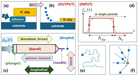
Meanwhile, let us turn our attention to our on-going research project. Here, we are assigned to help perform efficient underfill encapsulation for electronics industry. Figure 1(a,b) depict typical underfill encapsulation situations [29,30]. The goal is to provide adhesive solutions underneath an integrated circuit (IC) chip that is to be bonded to the underlying substrate. The overlapping arrow from Figure 1(a,b) indicates a decreasing feature size of an IC chip.
In older days, a bulk of adhesive fluid could have been pushed into the wide gap by an external force marked by ‘F’ on Figure 1(a). Conventional jetting of rather long liquid mass as illustrated on Figure 1(a) may be still employed for relatively coarse three-dimensional (3-D) printing [31]. When a miniature 3-D printer is employed for filling, say, very tiny holes, continuous liquid flow cannot fill in those holes because of large flow resistance per volume.
In recent days with ever-increasing miniaturization, the gap between IC chips and a substrate is so narrow that epoxy jetting or forced injection as shown on Figure 1(a) cannot accomplish adequate underfill encapsulation. Therefore, only sufficiently tiny droplets of adhesive solution are sucked into those thin gaps thanks to favorable capillary pulling force as shown on Figure 1(b) [29,30,32].
Concerning the modern-day underfill encapsulation illustrated on Figure 1(b), our task is to measure and control at real time the droplet dynamics of droplet dispensers so that certain specified volumes of droplets are ejected on demand [30,33,34].
Our experimental data let us believe that the dynamics at hand encompasses both fluid flows and structural deformation of a droplet dispenser on equal footing. Interactions between these two branches of mechanics are quite complicated so that we cannot analytically solve the relevant dynamics with high precision. Detailed numerical simulations are now available in literature on the whole or partial processes of droplet dispensing [7,30,35]. Although those details help us to understand what is going on, they cannot be utilized for real-time control of droplet dispensing [30].
Therefore, we decided to seek a simpler physical model for droplet dispensing. After several trials, we have learned that a telegraph-like equation and its solution could provide us with necessary clues as to the real-time controllability of a whole dispenser. Especially, the electric-circuit interpretation of the solutions to telegraph-like equations could help us to construct proper real-time measurement and/or control circuits [31,33,36].
In this connection, vibration control is an enabling technique not only in transportation vehicles and structural dynamics but also in manufacturing of semiconductor and precision machines [37]. In this respect, one of the goals of this study is to lay foundations on analytical tools that arise from telegraph-like equations. Such analytical tools could be utilized to enhance the functionalities of pertinent real-time control devices based on electric circuits that emulate telegraph equations [38].
Once those control devices are conFigured, we are trying to implement modern algorithms for physics-informed neural network (PINN) and/or physical AI (artificial intelligence) [32,39,40]. That is why we are frequently referring in this study to fundamental concepts underlying biological neuroscience [25,41]. We hope that this study contributes ultimately to realizing neuromorphic circuits [42].
Figure 1(c) illustrates a process of a single immunization shot administered through a medical syringe. Here, the driving force is exerted by hand pressure as given on Figure 1(c,d) [7,31,43]. For a proper injection shot, a nurse may have been trained, say, for a couple of months. Our droplet dispenser requires a certain total volume of droplets to be dropped over the chip area, after which the droplet dispenser is moved to another location over a substrate as shown by the trajectory on Figure 1(e). The whole encapsulation process is desired to be real-time automated. Consequently, our droplet dispensers are much harder to control than a single immunization injector shown on Figure 1(c).
Especially, the dynamics of droplet breakup and ejection should be adequately examined by taking into consideration capillarity, wetting, surface tension, and gravity [7,15,24,30,35,44,45]. Table 1 makes comparison among several fluid-ejection devices.
Here in this study, we will consider the fundamental aspects of the frequency dispersion relations of telegraph equations over infinite one-dimensional (1-D) domain [46]. Some of the characteristics found for telegraph equations are well-known. Notwithstanding, we focus on deriving those features not only from theorists’ perspectives but also from the perspective of practicing engineers.
Along this line of reasoning, section 2 provides reasons for why we examine telegraph equations from fresh look. Section 3 repeats the derivations of 1-D telegraph-like equations along with some reduced forms. Section 4 reexamines a 3-D telegraph equation for comparison to 1-D equations. Section 5 provides solutions to the well-known dispersion relation for the leaky telegraph equation. In addition, new findings including crossovers are offered for the dispersion relation of a leak-free telegraph equation. Section 6 handles the response functions for typical circuit configurations, thus showing features of low-pass filters. Section 7 offers some relevant discussions, followed by conclusions in section 8. Appendices are provided at the end to make this manuscript self-contained.
2. Motivation for this Study
As depicted on Figure 1(c), a droplet dispenser consists roughly of a plunger, a barrel, and a (contracting) nozzle [7]. An external forcing, say, compressed-air pressure is acting on the outside face of a plunger as illustrated on the left portion of Figure 1(c). Notice that the compressed-air excitation is just one of widely employed methods of periodically driving droplet dispensers [33,39,47]. As depicted on Figure 1(b), a droplet dispenser is employed for generating a stream of droplets of epoxy solution (being an electric insulator). This succession of droplets is dropped down on an electronic chip undergoing encapsulation process [30].
Let us denote the excitation by with being time. An idealized form of is displayed on Figure 1(d), where a single period out of repeated train of excitations is indicated by four segments of red lines [48]. As an initial stage, the infinitesimally short step-up event corresponds to pressurization. During the upper flat period , a main event of droplet ejection takes place. Afterwards, an infinitely short step-down event is enforced during which the ejection of a droplet is initiated and then terminated [31]. During the dormant or rest period , the droplet dispenser is moved to another position over a substrate as illustrated on Figure 1(e). Such a four-step process is repeated as designed. In our experimental runs, and , respectively.
Meanwhile, let us consider side conditions that consist of initial conditions (ICs) and boundary conditions (BCs) [1,2,19]. The damped vibration of a string of finite longitudinal length requires specifying certain valid boundary conditions (BCs). In addition, proper initial conditions are required for analytic solutions to telegraph equations [4,22,28,49,50]. Such Cauchy problems (PDEs and side conditions) for telegraph equations over finite 1-D domain will be handled in a separate publication.
In the meantime, Figure 2(a) illustrates a string of finite length , where a string in a quiescent state is just the horizontal green line along the longitudinal -direction (indicated by the horizontal double-headed arrow).
We will consider henceforth an infinite 1-D domain , although a finite length is introduced on Figure 2 for an illustrative purpose. Over time , this string could undergo lateral deformation in the lateral direction (indicated by the vertical double-headed arrow) perpendicular to the -direction. For instance, and indicate such lateral displacements at distinct times and on Figure 2(a). Both ends of the string are held fixed solely for illustrative purposes [14,15].
Let us copy the telegraph equation presented in [15] with slight alterations in notation as follows.
Here, is an internal damping and is Young’s modulus. In addition, the string parameters are the longitudinal tension, the mass per unit length, and the radius of a circular cross section of a string, respectively [16].
The first term on the left-hand side (LHS) of equation (1) signifies temporal decay. The wave equation made of two nearby terms on both sides of equality sign helps to determine the sound velocity of a string. This wave equation gives rise to propagating solutions consisting of a pair of functions for suitably differentiable forms of [2,14,19,25,27]. The last fourth-order term proportional to on the RHS stands for flexural (or bending) stiffness due to finite-sized cross section [7,10,11,12,14,24]. If this flexure term is neglected, equation (1) is reduced to the following.
Transient damping of a solid string of a finite radius could occur due to surrounding viscous incompressible fluid [13,22]. Here, one-way influence of a surrounding fluid flow on a string is assumed. Viscous drag by fluid on a solid gives rise to the first-order temporal-derivative term appearing in the above simpler telegraph equation. Furthermore, two-way fluid-structure interactions are handled in [8], where nonlinearities are hardly avoided. Such fluid-structure interactions play a crucial role also in underfill encapsulation [30], where thermal mismatches become often problematic.
Meanwhile, the influence of solid-tube deformation on the flow inside a tube is exploited for nondestructive ultrasonic measurement. Collapsible tube deformations that are dramatically larger than our minute deformations have been measured by ultrasonic techniques, where flows are maintained by applied pressure gradient as on Figure 1(c), Figure 2(b), Figure 2(c) and Figure 2(d) [51].
Pressure waves propagating through incompressible inviscid fluid inside a cylindrical elastic tube have been examined from diverse perspectives [8]. In this connection, let us turn to Figure 2(b–d), each of which displays a circular hollow tube of finite radius.
In terms of Cartesian -coordinates as on Figure 2(a), any radial direction on the -plane is called a lateral direction. In the cylindrical -coordinate as on Figure 2(b–d), the axial direction is pointing in the -coordinate, while the radial direction is pointing in the -coordinate. Inside each hollow tube lies a volume of fluid. The displacement components are provided along with their corresponding coordinates . In addition, the usual circumferential (azimuthal or angular) symmetry is assumed so that and the -dependences are suppressed.
Figure 2(b–d) correspond to distinct states of fluid flows and longitudinal pressure gradients as marked on each subfigure and summarized on Table 2. These pressure gradients result from the compressed-air excitation as depicted on Figure 1(c,d).
It is difficult in general to find analytical solutions to the fluid flow through a circular hollow tube of finite longitudinal length [4]. In this connection, recall that the solution to the unsteady Poiseuille flow has been constructed solely over a circular tube of infinite longitudinal length [52]. This fact makes all practical problems involved in droplet dispensers extremely difficult. Meanwhile, the momentum loss due to the shear stress between the inner wall of a cylindrical tube and internally flowing fluid can be considered as kind of leakage from the viewpoint of flowing fluid.
With both ends assumed fixed, no-flow case on Figure 2(b) exhibits a displacement profile that is symmetric across the central lateral plane. If downstream flow is set up as on Figure 2(c) thanks to favorable pressure gradient , the lateral displacements on the downstream half are greater on average than those on the upstream half. If upstream flow is set up as on Figure 2(d) due to unfavorable pressure gradient , the lateral displacements on the downstream half are smaller on average than those on the upstream half.
If temporal delay is neglected for simplicity, corresponds roughly to pressurization period, while corresponds roughly to depressurization period. Such periodic cycles consisting of pressurization and depressurization are executed by a pneumatic device for a droplet dispenser that is set up in our laboratory [33,34].
During unsteady transient processes as in our situations, Darcy-Weissbach law (the average longitudinal pressure gradient being proportional to the average fluid velocity squared) breaks down [51], thereby rendering extremely unpredictable the fluid flows inside a tube.
On Figure 2(c), we have illustrated the lateral displacements at two distinct locations, namely, and as indicated by the thick vertical lines and marked with 1Q (the first quadrant) and 3Q (the third quarter). To this end, we employed a modern nanoscopic optical displacement sensor, thereby measuring displacements on the order of sub-micrometer. In addition, the difference turns out to be temporally periodic as a response to periodic compress-air excitation.
Let us examine more closely the displacement fields of a circular tube as depicted on Figure 2(b–d). Also shown on Figure 2(b) are the radius (not a coordinate) of a tube and the tube thickness (not time). Suppose that such that the tube is relatively thin in comparison to its radius. Although the tube thickness is still accounted for, the displacement fields can be taken as being -independent. In this situation, the governing PDEs are the elastodynamic Navier equations [9,12].
In the thin-tube limit , Navier equations can be reduced to thin-plate equations for the two displacement components , which depend only on [10]. Such thin-plate equations play a crucial role in handling not only structural dynamics but also semiconductor thin films [50]. In our droplet dispensers, we expect so that we illustrate only on Figure 2(b–d). With these approximations, being of our primary concern stands for a bending mode, whereas stands for a pressure (‘p’ for short) mode. In comparison, a shear (‘s’ for short) mode is missing since we assumed [10]. Alternatively, is called an ‘out-of-plane displacement’, whereas is called an ‘in-plane displacement’.
Let us give a rough description of the reduced Navier thin-plate equations. Most importantly, these thin-plate equations possess the features of temporal transient, wave phenomenon, diffusion, leakage, and external source, namely, all features exhibited by the telegraph equation presented in equation (1). However, these reduced Navier equations contain partial differentials in addition to those partial differentials shown in equation (1). In other words, these reduced Navier equations are second order in time whilst they are fourth order in space in great distinction to the generix telegraph equations [7,24].
Quite importantly, the first-order derivative arises from the one-way fluid flows as depicted on Figure 2(c,d) during unsteady states. This presence of popping up in the reduced Navier equations lets the problem at hand be asymmetrical across the central lateral plane as illustrated by the spatial profile of the lateral displacement on Figure 2(c,d) [10].
However, both establishing proper BCs and finding associated analytical solutions to the thin-plate equations turn out to be significantly complicated. This is why we decided to examine a simpler telegraph equation in this study to explore the afore-mentioned compound effects. In this sense, we are seeking a ‘computationally minimal model’ for droplet dispensers [39].
3. Derivation of One-Dimensional (1-D) Telegraph Equation
We are taking conventional steps to derive a telegraph equation with the help of the electric circuit displayed on Figure 3(a) [31].
Figure 3(a) exhibits an electric circuit employed to derive a telegraph (a.k.a. telegrapher) equation [26]. Let us explain how this electric circuit is constructed in terms of electric potential and electric current from a generic perspective. From a narrower perspective of biological neurons, we can deal with the transmembrane potential and ionic current, respectively [38,39]. We assume that flow from left to right. Figure 3(a) shows an elemental domain over , where is the 1-D coordinate pointing to the right.
On Figure 3(a), there are four electric components: [i] a resistor of resistance , [ii] an inductor of (self-) inductance [3], [iii] a capacitor of capacitance , and [iv] an electric shunt conductor of the (leak) conductance (or the inverse of shunt resistance) [38,53]. They are also listed on Table 3 for summary.
Both and are longitudinally arranged, while and are laterally extended. An electric substrate can be considered as an environment, whereas the four-element circuit can be taken as a system. In case with usual electric chips, the conductance is considered as an unwanted leakage from a system to an environment. In fact, the encapsulation of electronic chips on a substrate serves two purposes: [i] a mechanical bonding, and [ii] an electronic insulation with selectively local electric conductions.
In this sense, our droplet dispensers need to properly establish encapsulation of electric chips onto a substrate as indicated by the trajectory of a dispenser on Figure 1(e). The electric conductance would be the resistance between those chips and a substrate.
Conductance plays also a key role in the analysis of neuronal signal transmission [25,41]. In terms of a biological neuron, an axon is directed along the longitudinal -direction, whereas a system normally implies the inside of an axon. The conductance accounts for the ions undergoing Ohmic processes through the transmembrane channels that connect laterally the inside of an axon and the environment consisting of extracellular space (ECS) [18,48]. While an axon can be considered as a system, the ECS can be taken as an environment. Meanwhile, the notion of ‘environment’ began to appear in [38].
From another viewpoint, a biological substrate can serve as an environment [45]. The system-environment interaction (SEI) is enabled by the transmembrane ion channels that laterally straddle the membranes of an axon. The inside of an axon is normally modeled as a cylindrical tube, the radius of which is normally much greater than the typical radius of ion channels. In practice, the membranes separating the inside of an axon from the ECS can be considered as porous walls.
In this respect, waves propagating through cortical circuits in-vitro experiments are believed to arise from synaptic interactions and the intrinsic behavior of local neuronal circuitry. This fact gives another credence to the validity of SEIs considered in this study [19].
The system consists of the resistor-inductor pair with , while the environment is everything other than the system as illustrated on Figure 3(a). Meanwhile, the capacitor-conductor pair with serves as bridges between the system and the environment, which is called in this study a ‘system-environment interaction (SEI)’. On Figure 3(a), both of the system elements are serially connected, whereas both of the SEI elements are arranged in parallel to each other.
Let us employ the symbol for a physical quantity ‘’. Because resistance and conductance are of inverse dimensions of each other, their product is dimensionless [17]. In Appendix A, we have proved that the following three products are of the following dimensions, where ‘’ is ‘second’ as a temporal unit.
It is worth stressing that the properties employed in this study are total values, which specify the off-the-shelf commodities available in stores selling electric components. In neuroscience, where the condition is mostly met, is called a ‘membrane time constant’ according to the dimension in equation (3).
For comparison with the data in literature, we define the per-unit-length properties as follows.
Throughout this study, is a certain constant length [20,25]. See Appendix A for numerical data of .
Meanwhile, Figure 2(a) shows as the string length measured in the -direction. In general, . The length is missing in almost all open literature available these days [20,26]. We find notwithstanding that the introduction of is necessary for setting up dimensionally correct formulas [17].
The electric potential undergoes reductions by due to a system resistor and by due to a system inductor. Meanwhile, the electric charge stored on the capacitor is given by . Therefore, the electric current through the capacitor is given by as the time-rate of charge. Likewise, for the (leak) conductance (or the inverse of shunt resistance [38,53], the electric current is given by [40]. It is crucial to notice that both leakage current components are directed from the system out to the environment. That is, we encounter two components of leakage (or escape) currents.
Resultantly, both and are governed by the first-order differentials over the length increment [25].
Here, we have added external distributed sources for potential and for current that are directed from the environment into the system [48,53]. For instance, is imposed by a patch electrode in neuroscience [39].
Combining both relationships in equation (5) leads to the following pair of second-order PDEs [1,2,26].
Here on the LHSs, the first terms stand for dissipation, while the second terms imply acceleration terms. On the right-hand sides (RHSs), the first terms signify diffusion, whereas the second terms refer to either leakage or forward reaction.
Such leakage is supposed to take place in the lateral direction as marked by the vertical double-headed arrow on Figure 1(c), Figure 2(a) and Figure 3(a). Since equation (6) contains diffusion only the longitudinal -direction, any lateral diffusion is not accounted for unlike the case in [27]. It is natural that the terms on each relation in equation (6) are of the same dimension. Meanwhile, is called a ‘membrane resistance’ especially for the term appearing in equation (6) [25].
When in equation (6) is interpreted to be a flow velocity as on Figure 2(b–d), the potential source can be taken to be proportional to the pressure , while is proportional to a pressure gradient . In this situation, the pressure at the entrance to the syringe of a droplet dispenser would be the excitation function depicted on Figure 1(c). In this study, the current source can be set to zero, i.e., .
Let us define a ‘full leaky RLGC circuit’, where a circuit with is differentiated from other circuits. A proper reference time for a full leaky RLGC circuit can be established in two ways when comparing two pairs of terms in the generic telegraph equation (6) as follows.
Here, superscript ‘’ and ‘’ signify the orders of the participating differentials, respectively.
Therefore, the strength of the leakage term can measured, in one way, by the above delay (or decay) time in equation (7) [4,7,19,38,53,54]. The dimensionalities listed in equation (3) can be employed to verify that the delay times carry indeed the dimension of time as shown in equation (7). Besides, corresponds to in equation (2].
Decay and delay are biologically plausible [38,48,55]. The numerator of consists of two terms, where each term is a product of a system parameter and a SEI parameter. Even the denominator of is another product of the two.
For the desired reference time , we can reconcile the two distinct reference times in equation (7) by taking their geometric average in the following manner.
This process of logically deriving a reference time has not been explicitly attempted elsewhere as far as we know. Since as a dimension, in agreement with the last formula in equation (3).
When source terms vanish, namely, , equation (6) is reduced to the following source-free ‘generic telegraph equations‘ [20,23].
Here, the two source-free equations are decoupled. Therefore, we will henceforth treat the first relation for the electric potential for convenience. The arrangement corresponding to equation (9) is schematically illustrated on Figure 3(b).
Equation (9) can be considered as either [i] diffusion equations contaminated by propagating waves [19], or [ii] wave equations contaminated by attenuation or damping [22,28]. Equation (9] is alternatively called a ‘propagative diffusion equation’ from the first viewpoint, whereas it is alternatively called a ‘damped wave equation’ from the second perspective [5].
Equation (9) can be alternatively cast into the following more familiar form when divided by [26,27].
Here, the conventional pair together with the signal velocity are defined. This equation is essentially identical to the simplified telegraph equation (2) valid for string vibration, except for the leakage term on the RHS of equation (10).
As summarized on Table 3, the ratios is a property of a system, whereas is a property of an SEI. Although these two ratios have already been identified in [26], their associations with a system and an SEI have never been properly entertained. Besides, both and belong to reactance.
Therefore, the product on the RHS of the last term in equation (10) is another manifestation of relative attenuation. In fact, corresponds to losses due to displacement-dependent lateral force for string vibration, but not due to externally applied lateral load for string vibration [37].
To cope with the pair more systematically, let us examine their ratio and the subsequent linear combination as follows.
Let us find the range of defined in equation (11) in the following manner.
Resultantly, for . Typical values of are evaluated for exemplary data in Appendix A [20].
By means of the parameters defined in equations (11) along with the properties in equation (12), we thus find that the condition is equivalent to the following alternatives.
Here, have been introduced in equation (10). Therefore, is equivalent to the equality , which is called the condition for ‘distortion-less propagation (but still not attenuation-less)‘ by [5].
Consequently, the condition of distortion-less propagation does not hold true in the special data of [56], which is experimentally measured for polyethylene insulated cable. A way of reaching the condition is to increase , which can be realized from the perspectives provided in Appendix B.
In this connection, let us take the following ratio between the two reference times and presented respectively in equations (7) and (8).
Here, is defined in equation (11).
In this respect, let us compare the magnitude of . To this end, we have drawn Figure 4 based on the data of [56], which are per-unit-length properties introduced in equations (4) and (5). Hence, and . We find here that approximately by two orders of magnitude.
Comparing equations (2) and (10), we ascertain the following correspondences.
In the spirit of introducing in equations (4) and (5), the signal velocity is employed throughout this study, where in view of in equation (3). In comparison, the formula widely employed in most of open literature employs the per-unit-length properties and in terms of our notation [26]. See Appendix A, which employs the per-unit-length properties of [20] for exemplary numerical evaluations.
It is crucial to notice in equation (15) that the tension is directed along the length of a string, while is the mass per unit longitudinal length [12]. Let us interpret the correspondence appearing in equation (15). The mass (inertia) per unit length carries the correspondence , where the capacitance per unit area is understood as sort of electric inertance. The remaining correspondence signifies the dynamical nature of both inductance and string tension .
Table 4 lists several relations reducible from equation (6).
As another easiest reduced case, consider the circuit with both internal-loss-free () and leak-free () properties. This wholly loss-free case is expected to cause no attenuation. In this case, the source-free generic telegraph equation (9) is further reduced to the following wave equation [2,12,55].
We call this PDE the ‘canonical wave equation’ [1,2]. Additionally, it is super-important to keep a non-zero capacitance and non-zero inductance in this case. Here, we have introduced a reference ‘LC time’, where the subscript ‘’ implies that . With reference to equations (15) and (16) for , according to equation (3).
Consider the following equation.
According to the four-element electric circuit depicted on Figure 3(a), equation (17) is at most hypothetical, since assumed for equation (17) requires that in equation (6). However, is impossible to achieve since .
Although this hypothetical equation (17) is not reducible from equation (9) by taking any proper combinations of the parameters , it shed light on further meaning of . As listed on Table 3, is the product of the two relative losses that represent respectively a system and a SEI.
Equation (17) is a simple harmonic equation described by, say, Hook’s law. Here, serves as an inertance (viz., effective mass) [37], while serves as an effective spring constant [12]. In this perspective, acts as a restoring force. Although the role of capacitance as an inertance is well-known, the role of as another inertance is less well-known.
The remaining special reduced case is the leak-free RLC circuit with (but not with ), whereby the source-free generic telegraph equation (9) is reduced to the following [4,13,22,49].
Let us call this equation a ‘leak-free diffusion-wave equation’, since it exhibits both diffusion and wave phenomena. Notice that there is still a loss due to the non-zero system loss, namely, . The absence of a leakage term in equation (18) corresponds to missing forward-reaction, if equation (18) is interpreted as a reaction-diffusion equation [38]. The arrangement corresponding to equation (18) is schematically illustrated on Figure 3(c).
Meanwhile, according to Figure 4, for a certain material. Therefore, the leak-free RLC circuit with is indeed an interesting limit case, identification of which is our own contribution.
Equation (18) has been derived by the analysis of two-dimensional (2-D) geometry in [3]. In addition to the longitudinal refence length , let be the lateral reference length. It is assumed in [3] that and under the approximation . Resultantly, , thereby getting in conformity with the expected dimension of on the RHS in equation (18).
In this connection, both equations (9) and (18) are 1-D hyperbolic-parabolic second-order equations [1,2,26], where wave propagations are implied by the adjective ‘hyperbolic’ and diffusion is implied by the adjective ‘parabolic’. The wave nature of the telegraph-like equations is what we are going to expand on in this study.
Let us reduce equation (6) into the following rotation-free (induction-free) leaky circuit with [17].
Hence, a wave-propagation feature is absent since , whence the signal velocity in equations (15) and (16) gets undefined. The PDEs in equation (19) are reaction-diffusion (a.k.a. diffusion-leak) equations, which are thus alternatively known as a ‘cable equation’ [25]. Notice in equation (19) that the second-order time derivatives and are absent. The arrangement corresponding to equation (19) is schematically illustrated on Figure 3(d).
The fact that the rotation-free leaky circuit with is apparently free of propagating waves as in equation (19) is suggestive of the fact that a non-zero inductance () is instrumental to supporting propagating waves [18,46]. As another example, dual propagation velocities (of different magnitudes but of the same sign) could prevail without attenuation in case with soliton flows involving surface tension [24].
In neuroscience, magnetic effects are normally neglected so that [48], albeit they are non-negligible in rare situations. Consider in equation (19) a special case that but for neuronal signal transmission. Furthermore, let us assume that with being a (spatially localized) delta function [19]. When the temporal portion is modeled by , where is what is shown on Figure 1(d). The resulting solution sought over a semi-infinite 1-D domain looks almost like what is presented in [48]. Notwithstanding, these solutions in [48] do not account for the termination stage involving drop ejection process [19].
A multi-variable extension of equation (19) with proper forms of excitations is well-known as a ‘leaky integrate-and-fire (LIF)’ model in neuroscience, where terms are leakage terms [19,25,36,38,39,41,42,53,54,57]. In case with the LIF model, the current source consists of either the sum or the integral from many other nearby neurons as depicted on Figure 1(f) showing convergent trajectories [19,25]. Here lies the connection between the subjects of droplet dispersers handled in our study and multi-layered neural network.
A heavily investigated form of equation (19) is its source-free diffusion-leak (reaction-diffusion) equation with as given below for an electric potential.
This special form of telegraph equation has also been extensively investigated as equation (19). This is also known as a ‘leaky heat equation’ [5], for which a heat-transfer aspect of the product is described in Appendix C [58].
We can define from equation (20) the ‘RC time’ by comparing the two terms and . The dimension from equation (3).
4. Derivation of Three-Dimensional (3-D) Telegraph Equation
As the last issue of the PDE, the telegraph equation (10) can be extended into 3-D space as follows in terms of conventional notation.
Here, introduced in equations (15) and (16). In addition, the -coordinate is along the longitudinal direction as marked by the horizontal double-headed arrow on Figure 1(c), Figure 2(a) and Figure 3(a). Therefore, the -plane is a lateral plane, being perpendicular to the longitudinal -axis. Besides, any radial direction on the -plane is a lateral direction. For equation (21) and the following relevant treatment, we closely follow [27].
Let us introduce below several parameters.
Here, form a complementary pair of characteristic curves, which stands for propagating waves [2]. Besides, is a real constant.
The solution to equation (21) assumes the following Ansatz of product form [57].
We are looking for a solution in the following special form.
This special form is satisfied for the parameters defined in equation (22), which help eliminate the term proportional in equation (24) as intentionally indicated by . This missing -term is indicative of leakage, the elimination of which corresponds to introducing an integrating factor for a differential equation as in [48].
Equation (24) is now handled with a method of separation of variables, thereby resulting in the following equation [2,52].
This special form is satisfied for the parameters defined in equation (22).
Equation (25) can be solved to provide a solution, whence the solution to can be further constructed according to equation (23).
Here, is yet another pair of constants.
Meanwhile, is the Airy function. Since Airy function is either sinusoidally attenuating or uniformly attenuating with increasing magnitude of its argument, the solution in equation (26) properly account for the spatially evanescent waves in the lateral direction as . In this connection, notice in equation (24) that the sum represents the diffusion on the lateral -plane.
Of course, there are both forward waves implied by and backward waves implied by in the solution presented in equation (26) [19,46]. Since equation (21) is symmetric in , we can easily come up with another equation involving instead of in equation (24) by replacing with in equation (21).
Both equations (20] and (25) are diffusion equations, where the longitudinal characteristic variable in equation (25) is time-like. As regards equation (9), we have already pointed out that telegraph equations harbor both features of diffusion and wave propagation.
A Cauchy problem for the diffusion-leak equation (19) has been solved with an appropriate set of side conditions early in 1946 by [48]. Although that diffusion-leak equation does not explicitly contain wave-propagation terms, the resulting solution in [48] contains implicit wave-propagation factors. Notwithstanding, the associated characteristic curves in [44] are not of the form but of nonlinear form in .
Notice furthermore that in equation (23) serves as sort of envelope function, which takes a slightly different form in [48] as well. In addition, it is worth recognizing that in equation (26) shows itself up not only in linear form but also in squared form.
Meanwhile, diffusion in equation (26) is manifested mostly by the Airy functions. In comparison, wave propagation is manifested by the two characteristic curves of , that appears not only in the Airy functions but also in the exponential function.
For a 1-D problem, equation (24) becomes , thus giving rise to a trivial solution for equation (23). For this 1-D problem, the solution in equation (26) is reduced to the following.
In comparison, the simplest wave equation in equation (16) admits a generic solution in the form of D'Alembert formula [1,2]. Here, are certain differentiable functions, while are certain constants depending on appropriate side conditions [4]. Consequently, the amplitude ratio between the forward waves with and the backward waves with will depend on the appropriate side conditions at hand [19].
5. Derivation and Analysis of Dispersion Relations
We mean by resonance the source-free conditions , for which the generic telegraph equation (9) is employed. Moreover, the wave amplitude on resonance is undetermined [46,57]. In this situation, in equation (9) are decoupled so that let us consider henceforth only .
Consider the Ansatz for propagating waves over the infinite domain . Here, denotes an imaginary unit such that . In addition, and are temporal frequency and spatial wave number, respectively [46,63]. As an aside, is called an ‘eikonal’ [63]. For example, small lateral displacements of a hollow tube in dynamic states as mentioned in section 2 guarantee the applicability of the above Ansatz [8,10].
There are two kinds of approaches to handling the propagation factor [12]: [i] the spatially attenuated and temporally periodic (SATP) approach [10,20,22,46], and [ii] the temporally attenuated and spatially periodic (TASP) approach [11,20,63]. In brief,
Here, and denote the real and complex spaces, respectively. Besides, the subscripts ‘’ and ‘’ denote the real and imaginary parts, respectively.
From our detailed study, the overall characteristics of the SATP approach turn out to be quite different from those of the TASP approach. The relevant algebra for the SATP approach is largely more complicated than that for the TASP approach [22].
With the TASP approach, we let be complex while keeping real, viz., and . With this TASP approach, problems valid over a finite 1-D domain such as on Figure 2 are easier to handle. One reason is that BCs at both ends are easier to specify [10,13] so that relevant boundary-value problems (BVPs) are easier to handle with the TASP approach.
With the TASP approach fully adopted, we have found many interesting phenomena. Among others, we rediscovered the well-known dual (double) attenuation rates for non-propagating stationary waves in addition to propagating waves [10,24,46,57,60]. Notwithstanding, finite-domain 1-D problems will be examined in a forthcoming publication, since the analysis is rather tricky. It is because several key findings such as cutoffs and crossovers would depend on the types of applicable side conditions.
In comparison, one of the advantages of the SATP approach in comparison to the TASP approach is the fact that temporally imposed functions such as displayed on Figure 1(d) can be easily resolved by way of, say, Fourier transform in with respect to .
Let us focus more on the SATP approach, for which we let be complex while keeping real [10,49].
Here, the inequality leads to the restriction that . Furthermore, notice that is the longitudinal wave number (a.k.a. propagation constant) directed along the longitudinal direction as marked by the horizontal double-headed arrow on Figure 1(c), Figure 2(a) and Figure 3(a).
With , we are looking for the existence of traveling waves [57]. Meanwhile, let us examine the propagation factor in more detail. On one hand, suppose that , whereby implies waves propagating into the positive -direction. Wave stability requires that as it progresses in view of the spatial-attenuation factor [11,13,20,22,57,63].
On the other hand, suppose the opposite case that , whereby implies waves propagating into the negative -direction. This negative propagation should carry . In brief, we should have in any case. The cases and are henceforth defined to correspond respectively to forward (propagating) waves and backward (propagating) waves. This way of interpreting the two cases and was exactly what has been adopted in [48].
Let us summarize below these two waves.
Telegraph-like equations and their solutions offer far-reaching applications in both mechanics and electric circuits. Suppose that the reaction-diffusion (or diffusion-leak) equation (18) is slightly modified by the addition of wave-propagation features exhibited by telegraph-like equations. Such slight addition would give rise to both forward and backward wave propagations as classified in equation (30) [25]. Here lies a possibility of arousing slight backpropagation in the characteristics exhibited by the conventional diffusion-leak equations [42].
Meanwhile, with this SATP approach, we could discover spatially evanescent modes if they are circumstantially admissible as discussed in the preceding section 4 [10]. In the sequel publication, our focus will be laid on how strong forward waves are in comparison to backward waves [19].
When the Ansatz in equation (29) is substituted into the source-free generic telegraph equation (9) [10], the following dispersion relation is obtained in two equivalent forms [22,46].
The arrangement corresponding to equation (31) is schematically illustrated on Figure 3(b).
It takes us by surprise that the generation of double (dual) attenuation peaks is hinged upon the resonance coupling between longitudinal and transverse (viz., lateral) resonators in the context of metamaterials consisting of simultaneous mass and stiffness [46]. In this regard, it is shown in [46] that the dual (double) attenuation rates carry two distinct contributions: [i] one rate stemming solely from system parameters that act in the longitudinal direction, and [ii] the other rate stemming from SEI parameters that account for both longitudinal and lateral dynamics.
It is rather disappointing to us that such a distinction made between a system and an SEI has not been explicitly recognized in [46].
Likewise, the dispersion relation in equation (31) exhibits a perfect symmetry between and so that the longitudinal system dynamics (represented by ) lies in interaction with the lateral SEI (represented by ). Moreover, in the interpretation by Hooke’s law in equation (17), the product ( from a system and from an SEI) serves as a mass and the other product ( from a system and from an SEI) acts as stiffness. See Table 3 for a summary in this respect.
At this juncture, let us introduce the following set of reference quantities and corresponding dimensionless parameters under the assumption of for a full leaky RLGC circuit.
Here, are dimensionless time and 1-D coordinate, respectively, while are dimensionless frequency and wave number, respectively.
As the most easily conceivable reduced case [19], the full leaky RLGC circuit with as illustrated on Figure 3(a) becomes a leak-free RLC circuit if and for which equation (18) holds true [49]. Let us examine the dispersion relation for this leak-free RLC circuit by setting in the generic equation (31) as follows.
This circuit with corresponds to an ideal perfect insulator, for which the shunt resistance becomes infinite [49]. Part of the reason why we examine this leak-free RLC circuit is the property as displayed on Figure 4. The arrangement corresponding to equation (33) is schematically illustrated on Figure 3(c).
As we did in equation (32), let us introduce a new pair of references and corresponding dimensionless parameters under the assumption of and for a leak-free RLC circuit.
Here, the tilde ‘~’ is employed as an overbar. Hence, are dimensionless time and 1-D coordinate, respectively, while are dimensionless frequency and wave number, respectively.
It is appropriate to examine the special ratio previously introduced in equation (34) in the following way.
Here, is the RC time previously defined in equation (20). Moreover, the reference-time ratio appearing in equations (34) and (35) complements the previously introduced ratio in equation (14).
Here, the reference time is identifiable also from equation (18) as another ratio in [22]. Besides, is alternatively called ‘an inverse of bandwidth’. In addition, has been identified in the context of interelectrode electric potential [49]. From mechanics viewpoint, is linked to viscous air resistance exerted on a vibrating string as illustrated on Figure 2(a).
In the meantime, the signal velocity employed in the simple wave equation (16) is linked to the following parameters respectively for the full leaky RLGC circuit and the leak-free RLC circuit.
Here, reference times and reference lengths are read respectively from equations (32) and (34).
Meanwhile, equations (31) and (33) are reduced to the following dimensionless forms respectively of and
Here, the parameter has already been defined in equation (11) with attendant properties in equation (12).
We have started with the four parameters in the PDE (9), which are readily reduced to two parameters in the PDE (10) [20]. We have identified in equation (37) that depends solely on a single parameter . Even better is the fact that is parameter-free.
Meanwhile, we resort to the following generic solution to for a generic [49].
When this formula is applied to equation (37), we obtain the following pair of solutions and [49].
Notice here that , while according to equation (29). Hence, the condition in equation (30) is satisfied. According to the generic formula in (38), the other solution is acceptable as well since . Therefore, we will stick to the solutions presented in equation (39) to fix the idea. Likewise, with .
Figure 5(a) displays two kinds of curves on the same display panel: [i] and in case of the full leaky RLGC circuit, and [ii] and in case of the leak-free RLC circuit. In addition, solid curves are drawn for the wave number or propagation constants and , while dashed curves are drawn for the attenuation rates and . Figure 5(a) is a zoomed-out version of Figure 5(a).
On one hand, let us examine the real parts and on solid curves. Both and are increasing with respective increasing frequencies. Meanwhile, notice from equation (12) that . In this connection, does not appear to be obtainable either from the limit or from the limit of . It is because the curve of lies between the curve of and .
On the other hand, let us examine the imaginary parts and on dashed curves. Once again, does not appear to be obtainable either from the limit or from the limit of. One aspect of these discrepancies is the following small-frequency limits as seen from equation (39).
Therefore, only is non-zero for any over , while other small-frequency limits vanish. These small-frequency limits and for any values of can be alternatively called ‘stationarity limits’ instead. These stationarity limits exhibit a significant phenomenon, since stands for non-propagating stationary state, which still undergoes spatial attenuation due to .
Recall that in the limit as shown in equation (40) by the SATP approach. We have carried out a separate analysis via the TASP approach (to be separately published) to find that in the limit is also achieved. Notwithstanding, we learn from the TASP approach a new phenomenon that there is a certain finite low-zone where . The TASP approach also revealed bifurcation phenomena for attenuation rates as well [19,57]. Such a finite forbidden wave-number zone cannot be seen via the current SATP approach. However, the significantly distinct behaviors between and in equation (40) are the symptom of the existence of such forbidden zones.
For the full leaky RLGC circuit, the following limits hold true for from the equation (39).
Therefore, is a straight line, while is a constant horizontal line as displayed by the red curves on Figure 5.
In brief, the curves of and exhibit rather distinct features in comparison to those of and . Especially, stationary non-propagating states do not appear to exist for the leak-free RLC circuit. The reason may be ascribed to the absence of dissipative SEIs for the leak-free RLC circuit with , namely, and [57].
This absence of stationary non-propagating states leads us to ask a self-question: “When an electric circuit is sufficiently insulated from an environment and hence an electric grounding is almost perfect, would then electric waves almost be always propagative rather than stationary?”. If this question were affirmatively answered, we might conjecture that ACs (alternating currents) will be better propagative through telegraph transmission lines than DCs (direct currents).
With reference to Figure 3(a), Table 5 makes comparison of several dispersion relations and corresponding key characteristics for the full leaky RLGC circuit with and other reduced circuits. Notice the reference length is undetermined. With a certain reference time , the ratio becomes a reference velocity.
In the meantime, the phase velocities and the group velocities are evaluated from equation (39) respectively via the following formulas [20,24,46,49,63].
Figure 6(a) displays two kinds of curves on the same display panel: [i] and for the full leaky RLGC circuit, and [ii] and for the leak-free RLC circuit. Here, and are phase velocities displayed on solid curves, while and are group velocities shown on dashed curves.
Overall, all solid curves increase uniformly with increasing frequencies, while all dashed curves exhibit local maxima at certain frequencies. For instance, a local maximum is pointed to by the green blank arrow on Figure 6(a) for . Such a maximum feature in the group velocity is not uncommon [49].
The curve of indicates a luminal phase velocity. All other phase velocities stay subluminal. In case with phase velocities, the inequality holds true over most of higher frequency zones except near zero frequency. However, such comparison between is not to be trusted due to distinct reference quantities listed in equations (32) and (34).
Each curve of group velocity exhibits a single crossover across the horizontal luminal line, e.g., as indicated by the green filled arrow on Figure 6(a) for . In other words, (subluminal) over , while (superluminal) over . Here, is a certain constant. Likewise, (subluminal) over , whereas (superluminal) over . The critical frequency appears to increase with increasing [19]. Besides, also displays a local maximum with respect to as clearly seen on Figure 6(b).
We can easily evaluate the zero-frequency limits of the phase and group velocities as follows based on equation (42).
We can confirm these limits easily on Figure 6(b). For instance, as indicated by the horizontal solid blue arrow on Figure 6(b). Also indicated by the green arrow near the coordinate origin is the limit . In addition, we have anomalous dispersion, namely, for and for all cases.
Meanwhile, consider the rotation-free leaky circuit with and as presented in equation (20). This circuit is devoid of wave propagation, since it is just a diffusion-leak equation. Therefore, the Ansatz is not applicable. Yet, let us continue to perform the following analysis of dispersion relation to see what kinds of difference exist between diffusion and wave propagation.
Here, on the RHS is linear in , while ’s on the RHSs of both equations (31) and (33) are quadratic in . This difference will lead to quite distinct behaviors of the respective dispersion relations. The arrangement corresponding to equation (44) is schematically illustrated on Figure 3(d).
Furthermore, let us handle the rotation-free (induction-free) leaky circuit with and as presented in equations (20) and (44) to prepare the following.
Here, we have introduced a ‘caret’ notation for this circuit. Additionally, we have introduced additional reference quantities . As discussed for Figure 4, , while is dimensionless as discussed in Appendix A.
We have examined in equation (36) whether the reference velocities and are equal to the well-known signal velocity . Therefore, making such comparisons with the help of in equation (45) turns out futile, because is undefined with . Therefore, conventional discussion in terms of subluminal, luminal, and superluminal states will become unfounded.
However, we can go on to find the dimensionless dispersion relation as follows based on equations (44) and (45).
Here, we have applied the square-root formula in equation (38), to explicitly find and as we have done in equation (39).
Based on equation (46), let us find the following pair of phase and group velocities as in equation (42).
Hence, we can easily come up with the following limit behaviors.
Here, the limit requires a bit of care in its derivation.
Figure 7 displays the dispersion characteristics against the dimensionless frequency . All members of increase uniformly with increasing without limits.
Notice that equation (20) is a diffusion-leak equation, thereby being endowed with no wave propagation. Therefore, both going without bounds as is indicative of infinite propagation velocity of signals especially for high frequencies. Such infinite propagation velocities are in conformance with, say, thermal heating being sensed instantly everywhere no matter how those senses are infinitesimally small. It is because governing equation for temperature is analogous to equation (20).
In mathematical languages, activities of parabolic PDEs carry infinite signal velocity. In comparison, hyperbolic PDEs such as in equations (9) and (18) are accompanied by finite propagation velocities as examined not only in equation (42) but also on Figure 5 and Figure 6 [1,2].
Such infinite propagation velocities are also in agreement with the finite group velocity in equation (48) at a stationary state. It is because a group velocity is sort of energy-transmission velocity, by which wave energy is steadily supplied for all temporally neighboring transient states of non-zero frequencies. The non-zero finite attenuation rate in equation (48) at a steady state also agrees with such energy transfer in low frequencies beginning with zero frequency.
A further reduction of the case with is that for the rotation-free and leak-free circuit. For this circuit, equation (31) is reduced to provide the following.
Here, we have introduced yet another set of notations with inverted arc.
Moreover, a new reference time is defined. This time is deducible from equation (33) such that it been conventionally called an ‘RC (membrane) time’ in the context of neuroscience [38,39] and diffusive memristors [43]. This nomenclature is made in comparison to the LC time inequation (16), which is also easily deducible from equation (33) on dimensional ground.
Furthermore, we have pointed out that the absence of in equation (49) leads to a different signal velocity as for the rotation-free laky circuit discussed in equation (45).
We can easily find the solution to in equation (49) as follow by way of the generic formula in equation (38).
Here, the solution led easily to the corresponding phase and group velocities given above. Resultantly, both phase and group velocities are constant with respect to the non-dimensional scheme provided in equation (49).
Starting with equation (31), we process for the internal-loss-free and leak-free circuit with and to obtain the following.
These results are simpler than those in equations (49) and (50). The linear dispersion relation is what we have discussed in equation (16) for the canonical wave equation.
In this case, we end up with the ratio , thus being the signal velocity introduced in equation (16). Resultantly, both phase and group velocities are luminal for all frequencies.
6. Response Functions of Single Four-Element Electric Circuits
Let us consider another leaky circuit consisting of four discrete electric elements with . Figure 8 illustrates two distinct circuit arrangements, which are variants of the full leaky RLGC circuit displayed on Figure 3(a). Both arrangements in Figure 8 share the same pairs of SEI components, namely, a capacitor with and a conductor with that are connected in parallel to each other. This subcircuit is then linked to a system consisting of an inductor with and a resistor with . The difference is that and within a system are connected in series with each other on Figure 8(a), while they are arranged in parallel to each other on Figure 8(b).
See equation (4) for the relationships between dimensional and dimensionless parameters. While the per-unit-length properties are appropriate for the continuous electric circuit on Figure 3(a), the total properties are certainly appropriate for the discrete electric circuit on Figure 8.
For each configuration, our goal is to find the (frequency) response function , being the ratio of the output electric potential against the input electric potential . Here, is a common ground potential, being held constant [38]. For simplicity, we neglect any spatial dependences unlike the case with Figure 3(a) so that only temporal dynamics will be considered. We thus do not need a reference length here.
In addition, notice that the two SEI elements carry electric currents , respectively. According to Kirchhoff’s circuit law of conservation of electric currents, we have . Hence, the following pair of relations hold true [38].
Here, we have applied the Ansatz for temporal periodicity of dynamics.
Let us make analysis of the serial system shown on Figure 8(a) as in equation (53).
Combining in equation (53) and in equation (54) leads to the following response function.
Let us turn to the parallel system displayed on Figure 8(b) as follows by way of , being different from equation (54).
Combining in equation (53) and in equation (56) leads to the following response function for the parallel system.
Meanwhile, let us invert in equation (11) as follows.
Therefore, is doubly valued in . Hence, it will be better to employ whenever both of show up in the forthcoming formulas.
Let us make dimensionless both complex response functions (for serial system) and (for parallel system), respectively in equations (55) and (57) as follows [19].
Here, we have employed the following intermediate relationships based on the various parameters presented in equations (11) and (32).
Notice again that the product is dimensionless as provided in equation (3). This way of comparing serial and parallel circuits is crucial to properly assessing the performances of electrical devices useful in practice [62].
Normally, what we need are the following magnitudes.
Large- limits are easily found below.
Hence, the serial system exhibits an inversely linear behavior with respect to , while the parallel system exhibits an inversely quadratic behavior with respect to .
Figure 9 shows the magnitudes of response functions plotted against the dimensionless frequency for varying values of . For a given value of , each subfigure displays that over all range of . In words, a parallel system undergoes a less potential drop than a serial system while the SEIs remain the same.
Most of the response functions exhibit maxima at zero frequencies (namely, static states), thus standing for low-pass filters [10]. One exception is the dotted green curves for with , where a maximum takes place at a non-zero finite . Other curves of red, black, and blue colors exhibit uniform decreases with increasing . Besides, the curves of are identical with those of thanks to the factor appearing in equation (61).
The four subfigures of Figure 9 show that the high-frequency components are especially damped with increasing as also observed by [38] in their numerical solution with a LIF model. Leakages help a system under consideration to become robust (namely, stable) against perturbations although leaks are incurred [57].
In this regard, consider a temporally periodic function where each cycle consists of two step changes and a flat period in between, followed by a dormant period as displayed on Figure 1(d). Suppose further that such temporal discontinuities are resolved into various frequency components according to Fourier decomposition [62]. In view of Gibbs’ phenomenon for such a decomposition, there appear unwanted high-frequency components that get stronger across discontinuities [31]. The low-pass (temporal) filter as shown on Figure 9 dampens faster-oscillating components by greater amount than slower oscillating components [25].
In this respect, the large- behaviors in equation (62) are also visible on Figure 9, where stronger temporal attenuations with increasing are exhibited for a serial system in comparison to a parallel system. Such a low-pass filter capability would have been associated with non-zero values of the inductance . This reasoning is based on the dispersion features displayed on Figure 7 obtained for the rotation-free leaky circuit with and , where ever-increasing relation is shown up to infinitely high frequencies.
The discontinuous step-up and step-down processes illustrated by the red lines on Figure 1(d) model an idealistic situation. Instead, we suppose in practical situations that continuous ramp-up and ramp-down processes indicated by the blue dotted curves on Figure 1(d) are more likely to take place [33,40,50,51,62]. For that kind of temporally continuous forcing, the portion of the high-frequency response will be of less nuisance. A disadvantage is that the entire analysis would require numerical solutions for such continuous forcing functions.
It is seen from Figure 9 that a parallel system is more efficient than a serial system in acting as a low-pass filter. In this respect, it is well-known that a central processing unit (CPU) works mostly via serial processing, while a graphical processing unit (GPU) functions via parallel processing. We are then faced with our own question as to whether a GPU serves as a generically better low-pass filter than a CPU. This question remains to be answered in our future publications.
In this respect, let us consider the serial system displayed on Figure 8(a), where the two elements are repeated in a serial manner as indicated by the horizontal double-headed green arrow. To find the pertinent response function, we need to modify the system given in equations (53), (54), and (55) in the following manner.
Here, the superscript ‘’ indicates a repetition number.
We find that in equation (63) is obtainable by making substitutions and into in equation (55), thereby satisfying the usual recipe for serial extension.
Likewise, let us consider the parallel system displayed on Figure 8(b), where the two elements are repeated in a parallel manner as indicated by the vertical double-headed green arrow. To find the pertinent response function, we need just to modify the system given in equations (56) and (57) in the following manner.
Therefore, in equation (64) is obtainable by making substitutions and into in equation (57), thereby conforming to the usual recipe for parallel juxtaposition.
According to the ways that and are defined respectively in equation (11) and (32), both and remain unaltered even under the serial extension and the parallel juxtaposition. Consequently, the dimensionless forms in equations (63) and (64) are easily modified to the following.
Hence, we get to the following large- limits.
Here, and are what have already been presented in equation (62), which corresponds to with a single pair of .
Notice that the response functions and have been derived by neglecting all spatial variations, while keeping only temporal variations. Notwithstanding, the error incurred by the serial extension for gets more serious due to, say, the temporal delay presented in equation (7). In comparison, the error incurred by the parallel juxtaposition for would become minimal thanks to the same longitudinal extension. Therefore, becomes less reliable as is increased, while stays relatively reliable even with creasing .
Equations (65) and (66) tell that is uniformly decreasing with increasing . In comparison, appears to be rather fuzzy with varying . Therefore, Figure 10 displays with two values of . We learn from Figure 10 that if . In comparison, and undergo a crossover with varying if as seen by the pair of green curves, which is marked by a black blank circle and pointed to by a black solid downward arrow on Figure 10.
We have examined the balance between and in equation (7) in coming up with . Let us find below the condition that these two terms are equal in magnitudes in terms of the frequency defined in equation (32).
Here, we have utilized and , which have been introduced in equation (32). Therefore,
The critical frequency is evaluated below for example.
Let us take for both of which . This dividing critical frequency is indicated on Figure 10 by the green vertical dotted line. Figure 10 marks the left region by ‘decay-dominated’, while it marks the right region by ‘wave-dominated’. In brief, low-pass filters favor decay-dominated temporal dynamics.
7. Discussion
To get closer to reality, we need to consider telegraph equations over a finite 1-D domain as on Figure 2 [49]. For that purpose, proper boundary conditions (BCs) should be assigned for problems valid over a finite 1-D domain [28,50]. To this goal, in-depth analysis of the relevant BCs is required to reflect the physical situation at hand in our project [4].
What we expect from the resulting solutions to the telegraph equation over a finite 1-D domain is the relative strength between forward waves and backward waves [42]. From this viewpoint, the unequal strengths of forward and backward waves are determined by the ratio between in equation (27). This ratio is undetermined since in equation (27) is still undetermined. Actual values of should be determined by applying appropriate side conditions [42].
Such distinct wave velocities are in sharp contrast to the form as a solution to the idealized hypothetical equation (16). We suppose that a proper set of BCs at both ends of a finite-length tube such as on Figure 2(b–d) should properly reflect the moving plunger at the upstream and the droplet ejection dynamics at the downstream end as depicted on Figure 1(c). Following an analogous line of reasoning, we conjecture that backward waves are associated with the backlash occurring with 3-D printing [32] and/or the suck-back phenomenon associated with the end-phase ejection of droplets being issued outward from droplet dispensers [7].
In this connection, the forward wave is generated by stimulating a previously inactive region, whereas the backward (reverse) wave is initiated by removing stimulation from a previously active region [19].
As crudes approximations, either Neumann condition or Dirichlet condition could be chosen [2,12,28]. However, when a mixed-type BC with generic complex coefficients is admitted, selections of physically admissible BC will get intricate. Here comes the notion of feedback due to the BC at the downstream end, by which the whole upstream dynamics may be significantly affected [45]. Moreover, the tube displacements shown on Figure 2(b–d) in the longitudinal direction should also be accounted for in a more realistic situation [12], thereby demanding more delicate BCs.
Solving the 3-D telegraph equation valid over the whole space as discussed in section 4 will be challenging when a problem domain is chosen either the inside or the outside of a circular cylindrical hollow tube of finite axial length. In this case, the Cartesian coordinates employed in section 4 should be replaced with cylindrical coordinates in handling the pertinent differential equations. Even the circumferential independence is assumed, this 3-D telegraph equation will be hard to solve depending on the necessary side conditions.
Last but not the least, the telegraph equations modified for droplet dispensers will be examined by consulting our experimental measurement data in a separate publication.
8. Conclusions
We have not only collected well-known fundamental properties of telegraph equations but also identified so-far hidden characteristics. Interactions between a system and an environment shed new light on the notion of leakage not only in mechanical vibration but also electric circuits. Especially, crossovers are found to take place for the phase and group velocities. We hope this study will help us in the future to set up real-time control devices and attendant control software for droplet dispensers employable for practical underfill encapsulation of integrated circuit chips. In this respect, we performed fundamental studies on propagating waves that carry information back and forth with unavoidable decays.
Author Contributions
Conceptualization, S.-H. Kim and H.-I. Lee; methodology, S.-H. Kim and T.-Y. Kim; software, T.-Y. Kim; validation, S.-H. Kim and T.-Y. Kim; formal analysis, H.-I. Lee; investigation, S.-H. Kim, T.-Y. Kim and H.-J. Moon; resources, S.-H. Kim; data curation, S.-H. Kim and T. Y. Kim; writing—original draft preparation, H.-I. Lee; writing—review and editing, H.-I. Lee and H.-J. Moon; visualization, T.-Y. Kim; supervision, H.-J. Moon; project administration, H. Moon; funding acquisition, H. I. Lee and H.-J. Moon. All authors have read and agreed to the published version of the manuscript. The importance of structural vibration examined in section 2 has been suggested especially by S.-H. Kim, thereby playing a crucial role in the whole project.
Funding
This research was funded by the Commercialization Promotion Agency for R&D Outcomes (COMPA) funded by the Ministry of Science and ICT (MSIT), grant number 2710084647, under the subject of ‘Development of Non-invasive Real-time Flow-Rate Measurement Systems for Droplet Dispensers Employed for Smart Process Automation of Semiconductor Manufacturing’.
Informed Consent Statement
Not applicable
Data Availability Statement
The dataset generated during and/or analyzed during the current study is available from the corresponding author on reasonable request.
Conflicts of Interest
The authors declare no conflicts of interest.
Abbreviations
The following abbreviations are used in this manuscript:
| 1-D | One-Dimensional |
| 2-D | Two-Dimensional |
| 3-D | Three-Dimensional |
| BC | Boundary Condition |
| LHS | Left-Hand Side |
| PDE | Partial Differential Equation |
| RHS | Right-Hand Side |
| SATP | Spatially Attenuated and Temporally Periodic |
| SEI | System-Environment Interaction |
| TASP | Temporally Attenuated and Spatially Periodic |
Appendix A. Reference Times and Properties of Circuit Elements
Let us employ the MKS unit system, where MKS denotes ‘meter-kilometer-second’. We will employ the symbol for a physical quantity ‘’ as in equation (3). We can read from standard textbooks the dimensions of as given below.
By definition, means that the dimension of resistance is inverse of the dimension of conductance. Moreover, is ‘Ampère’ as the unit of electric currents. The dimensions of the products are easily found as follows.
We have thus proved that and as claimed in equation (3).
In addition, we obtain the following relationships from equations (7) and (11).
As a complement to in equation (35), let us define another ratio as follows based on in equation (34) and in equation (16).
Here, is alternatively called a ‘Q-factor’, being an inverse of fractional bandwidth.

Table A1.
Frequency-dispersive data for the four circuit components
| symbol | name | status | Frequency dispersion |
| Resistance | system | ||
| inductance | system | ||
| conductance | SEI1 | ||
| capacitance | SEI1 | ||
| spring | system | ||
| inertance | SEI |
1 SEI (system-environment interaction).
Figure A1.
(a) and versus . (b) along with and versus . The common horizontal coordinate is not to scale, where the numbers correspond respectively to in units of Hertz. The per-unit-length properties are provided such that in (Ohm per kilometer), in (micro-Henry per kilometer), in (Siemens per kilometer). All data is taken from [56].
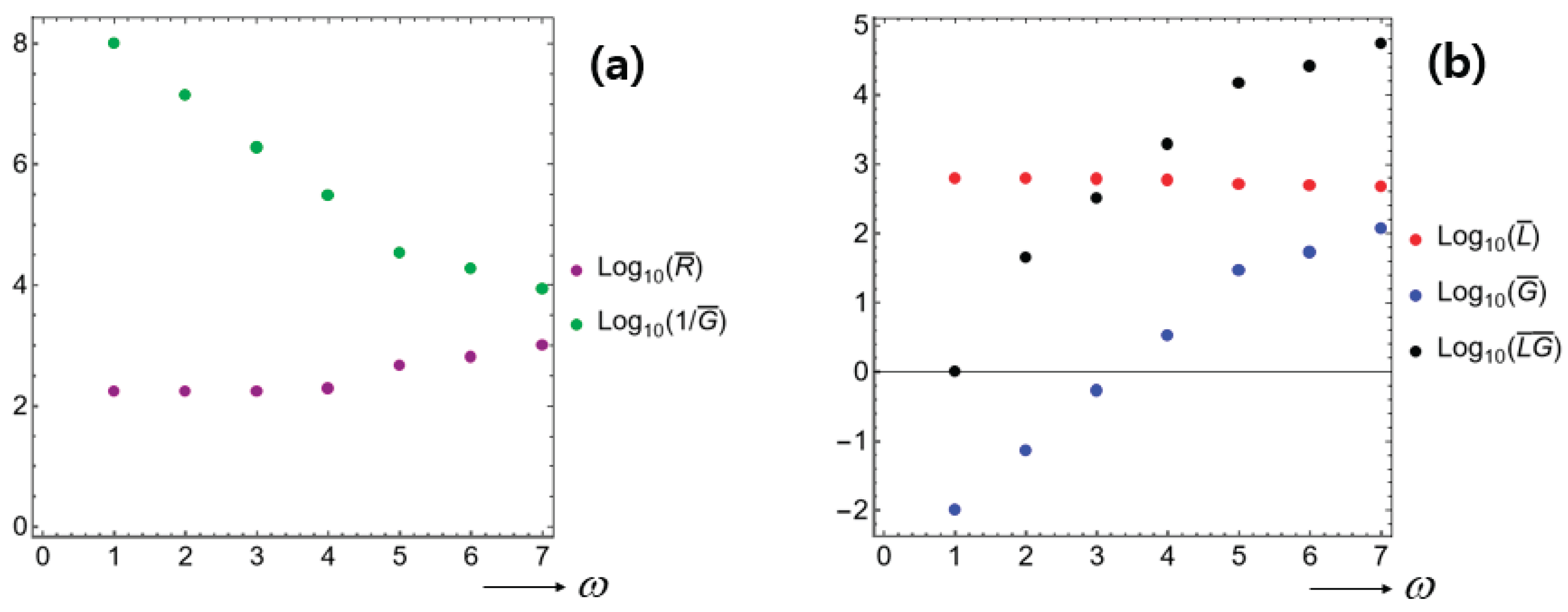
In general, all of could depend on the state, namely, as functions of , thereby making the PDEs in equation (6) to be nonlinear. From another perspective, we can think of in terms of temporal frequency , thereby meaning frequency-dispersive properties. According to the data of [56], the unavoidable capacitor turns out to remain largely constant even with varying frequency. In comparison, , , and . These findings on frequency-dispersive data are summarized on Table A1.
We have drawn Figure A1 based on the data of [56], which offers per-unit-length properties . We learn from this Figure that over most , thus signifying that the intrinsic system loss is greater than the SEI loss . However, decreases with increasing , thereby indicating that high-frequency behaviors might be different from the low-frequency behaviors. Since both decrease with increasing according to Figure A1(a), the effective spring constant in the last term on the RHS of equation (17) is likely to decrease with increasing .
In terms of , is associated with the Lorentz force so that increasing the system inductance could lead to a decrease in the channel conductance . Meanwhile, Lorentz force causes an increase in friction that hampers ionic flows inside the ionic channel through a neuronal membrane [55,64]. Such increased friction accounts for a reduction in the (shunt) conductance (viz., an increase in the shunt resistance [49,53] of the channel when compared with ions flowing in bulk media. Therefore, the product has a higher probability of staying constant [18].
Table A1 lists that and so that the product has a higher probability of staying constant. To this goal, Figure A1(b) shows along with and . We find here that the variation in is much stronger than the variation in , thus resulting in non-constant product . Yet, we suppose that industrial electric components could be constructed such that the product remains near-constant. Further discussion on how to make variations in is provided in [53].
Consider the following per-unit-length properties provided in [20].
Here, is ‘Ohm’, being the unit of resistance (not being dimensionless frequency as in most of the main body of this manuscript).
Consider and introduced in equation (11). Since this data is specified per unit meter, we can employ it to evaluate in the following way.
Hence, turns out rather small in this example of [20].
Furthermore, consider the units of and examined in equations (10), (13) and (35) as follows according to the units in equation (A1).
Notice especially that .
Appendix B. Three-Dimensional (3-D) Effects and Memristors
See the Cartesian -coordinates for the four-element electric circuit shown on Figure 3(a). Suppose that two Helmholtz coils are wound respectively around the longitudinal -axis. These two coils are arranged in parallel to each other. Magnetic fields established by Helmholtz coils induce electric currents along the longitudinal -axis [18]. The magnetoreception in humans might have been based on such a principle [59].
Likewise, a system inductance could be established due to the magnetic-field effect which involves two-dimensional (2-D) rotational magnetic field on the lateral -plane around the -coordinate [61].
Let us comprehend the meaning of that is readable from equation (15), with being the string tension employed in equation (1). To this end, let us rewrite the usual relationship constituting equation (5) into so that the inverse inductance acts like a "tension" in the sense that it resists changes in current flow, similar to how a physical tension resists the stretching of a string.
For a given voltage drop across a given inductor, the increasing magnetic field (or inductance) wound along the longitudinal axis of (an) inductor coil(s) hinders an induced electric current flowing along the longitudinal axis. For instance, in case with a gas plasma under the influence of a vortex-like rotational magnetic field of strength , the resultant inductance is inversely proportional to [49]. In other words, an inductor serves as an arresting agent rather than as a promoter (enhancer) [60].
From another viewpoint, inductance arises from truly 3-D effects. In comparison, capacitor involves two facing (flat) areas lying perpendicular to the longitudinal axis, thereby being caused by a 2-D effect. In another comparison, resistance appears to arise from a relatively 1-D effect along the longitudinal axis. However, a thin conducting wire incurs its resistance mostly along its outside surface so that resistance is also caused by non-1-D effects in real devices. See the summary on table 3.
We have so far dealt fundamentally with three elements of , since is an inverse resistance. A fourth element is memristor (memory resistance), which requires nonlinear analysis in association with double-loop hysteresis [40,50]. The magnetic flux that influences the inductance is related to the memristance (the property of a memristor). Therefore, full electromagnetics principles play active roles in completing the dynamics for One of electric circuits constructed so far involves a resistor and a memristor [43], where time delay is incurred due to a resistance as in equations (13) and (14). In both [40] and [43], pulses of electric potentials are examined either in the discontinuous form as marked by the straight lines on Figure 1(d) or in the continuous form as marked by the dashed curves on Figure 1(d) [62].
If the electric-circuit model depicted on Figure 3(a) is modified by the insertion of memristor, a question arises as to how the telegraph equation (6) will be accordingly modified. This question becomes vitally important with decreasing size of electronic chips and in highly dynamic states as with switching events [50]. We will explore this aspect in our future publication.
Appendix C. Convective Heat-Transfer for Leakage
To clarify the meaning of leakage of the terms in equation (6), let us assume temporarily that denotes temperature of a system, while the constant as appears on Figure 3(a) is equal to the environmental temperature. Besides, we assume that . The equation for is then modified into the following.
Hence, temperature is measured based on . Therefore, the leakage term could model the lateral heat loss from a system into an environment, which is alternatively called ‘Newton’s cooling law’ [43]. Here, serves as a convective-heat-transfer coefficient [58]. Suppose that a hotter fluid flows inside a cylindrical hollow tube as shown on Figure 2(c,d), while the outside of the tube is a cooler air environment. The convective heat transfer between the outside wall and the air depends approximately on the difference , with accounts for all flow conditions on the outside of the tube [38].
In this interpretation, the source term on the RHS of equation (6) signifies an imposed temperature gradient in the longitudinal direction, thus being analogous to the imposed pressure gradient indicated on Figure 2(c,d). This situation constitutes one of additional research projects in our company.
Equation (18) has also been identified from the perspective of heat transfer [22], whereby stands for thermal relaxation (for instance, the Maxwell-Cattaneo rule).
References
- Stone, M.; Goldbart, P. Mathematics for Physics: A Guided Tour for Graduate Students; 1st Edition; Cambridge University Press: Cambridge, U.K., 2012; pp. 193–294. [Google Scholar] [CrossRef]
- Pinchover, Y.; Rubinstein, J. An introduction to Partial Differential Equations; 8th printing; Cambridge University Press.: Cambridge, U.K., 2013; pp. 76–129. ISBN 978-0-521-84886-2. [Google Scholar]
- Assis, A.K.T.; Hernandes, J. A. Telegraphy Equation from Weber’s Electrodynamics. IEEE Transactions on Circuits and Systems – II: Express Briefs 2005, 52(6), 289–292. [Google Scholar] [CrossRef]
- Gugat, M. Boundary feedback stabilization of the telegraph equation: Decay rates for vanishing damping term. Systems & Control Letters 2014, 66, 72–84. [Google Scholar] [CrossRef]
- Donaghy-Spargo, C. On Heaviside’s contributions to transmission line theory: waves, diffusion and energy flux. Phil.Trans. R. Soc. A 2018, 376, 20170457. [Google Scholar] [CrossRef] [PubMed]
- Kanatani, K.; Ogasawara, T.; Toh, S. Telegraph-Type versus Diffusion-Type Models of Turbulent Relative Dispersion. J. Phys. Soc. Jpn. 2009, 78, 024401. [Google Scholar] [CrossRef]
- Mehrabian, H.; Feng, J.J. Auto-ejection of liquid drops from capillary tubes. J. Fluid Mech. 2014, 752, 670–692. [Google Scholar] [CrossRef]
- Abulwafa, E.M.; El-Shewy, E.K.; Mahmoud, A.A. Time-fractional effect on pressure waves propagating through a fluid filled circular long elastic tube. Egyptian Journal of Basic and Applied Sciences 2016, 3(1), 35–43. [Google Scholar] [CrossRef]
- Graff, K.F. Wave Motion in Elastic Solids; Dover Books on Physics, Dover Publications: New York, U.S.A., 1991; pp. 9-74 and pp. 213-272. [Google Scholar]
- Brewer, C.; Creagh, S.; Tanner, G.K. Elastodynamics on graphs - wave propagation on networks of plates. J. Phys. A: Math. Theor. 2018, 51, 445101. [Google Scholar] [CrossRef]
- Meng, Q.; Shi, Z. Propagation Attenuation of Plane Waves in Single-Phased Soil by Periodic Pile Barriers”. Int. J. Geomech 2018, 18(6), 04018035. [Google Scholar] [CrossRef]
- Lee, D.; Oh, J.H.; Kang, I.S.; Rho, J. Seismic phononic crystals by elastodynamic Navier equation. Physical Review E 2019, 100(6), 063002. [Google Scholar] [CrossRef]
- Lin, S.P. Damped vibration of a string. Journal of Fluid Mechanics 1975, 72(04), 787. [Google Scholar] [CrossRef]
- Chaigne, A.; Askenfelt, A. Numerical Simulations of Piano Strings I: Physical Model for a Struck String Using Finite Difference Methods. J. Acoustical Soc. Am. 1994, 95(2), 1112–1118. [Google Scholar] [CrossRef]
- Giordano, N. On hearing the ‘shape’ of a vibrating string. Computing in Science & Engineering 2002, 4(3), 100–105. [Google Scholar] [CrossRef]
- Perov, P.; Johnson, W.; Perova-Mello, N. The physics of guitar string vibrations. American Journal of Physics 2015, 84(1), 38–43. [Google Scholar] [CrossRef]
- FitzHugh, R. Dimensional analysis of nerve models. J. Theor. Biol. 1973, 40, 517. [Google Scholar] [CrossRef]
- Freire, M.J.; Bernal-Méndez, J.; Pérez, A.T. The Lorentz force on ions in membrane channels of neurons as a mechanism for transcranial static magnetic stimulation. Electromagn Biol Med. 2020, 39(4), 310–315. [Google Scholar] [CrossRef]
- Coombes, S.; Owen, M.R. Evans Functions for Integral Neural Field Equations with Heaviside Firing Rate Function. SIAM Journal on Applied Dynamical Systems 2004, 3(4), 574–600. [Google Scholar] [CrossRef]
- Cohen, L.; Loughlin, P. Phase Space Analysis of the Telegraph Equation. IEEE Transactions on Antennas and Propagation 2022, 70(10), 9687–9693. [Google Scholar] [CrossRef]
- Barna, I.F.; Kersner, R. Heat conduction: a telegraph-type model with self-similar behavior of solutions. J. Phys. A: Math. Theor. 2010, 43 375210. [Google Scholar] [CrossRef]
- Zhang, D.; Ostoja-Starzewski, M. Telegraph equation: two types of harmonic waves, a discontinuity wave, and a spectral finite element. Acta Mech 2019, 230, 1725–1743. [Google Scholar] [CrossRef]
- Arbab, A.I. Quantum Telegraph equation: New matter wave equation. Optik 2017, 140, 1010–1019. [Google Scholar] [CrossRef]
- Irwaq, I.A.; Alquran, M.; Jaradat, I.; et al. New dual-mode Kadomtsev–Petviashvili model with strong–weak surface tension: analysis and application. Adv. Differ. Equ. 2018, 2018, 433. [Google Scholar] [CrossRef]
- Bressloff, P.C. Spatiotemporal dynamics of continuum neural fields. J. Phys. A Math. Theor. 2012, 45(3), 033001. [Google Scholar] [CrossRef]
- Srivastava, V.K.; Awasthi, M. K.; Chaurasia, R. K.; Tamsir, M. The Telegraph Equation and Its Solution by Reduced Differential Transform Method. Modelling and Simulation in Engineering 2013, 2013, 746351. [Google Scholar] [CrossRef]
- Asenjo, F.A.; Hojman, S.A.; Villegas-Martínez, B.M; Moya-Cessa, H.M.; Soto-Eguibar, F. Exact solutions to the Telegraph equation in terms of Airy functions. Revista Mexicana de Física 2024, 70, 040701. [Google Scholar] [CrossRef]
- Asif, M.; Bilal, F.; Haider, N.; et al. Robust numerical techniques for modeling telegraph equations in multi-scale and heterogeneous environments. J. Appl. Math. Comput. 2025, 71, 6585–6620. [Google Scholar] [CrossRef]
- Zhang, Z.; Wong, C.P. Recent Advances in Flip-Chip Underfill: Materials. IEEE Transactions on Advanced Packaging 2004, 27(3), 515. [Google Scholar] [CrossRef]
- Ng, F.C.; Abas, M.A. Underfill Flow in Flip-Chip Encapsulation Process: A Review. Transactions of the ASME Journal of Electronic Packaging 2022, 144, 010803–1. [Google Scholar] [CrossRef]
- Pinar, A.; Wijnen, B.; Anzalone, G.C.; Havens, T.C.; Sanders, P.G.; Pearce, J.M. Low-Cost Open-Source Voltage and Current Monitor for Gas Metal Arc Weld 3D Printing. Journal of Sensors 2015, 2015, 876714. [Google Scholar] [CrossRef]
- Vajda, J.; Banović, L.; Miško, M.; Drstvenšek, I.; Milojević, M.; Maver, U.; Vihar, B. Algorithmic linearization improves Syringe-based extrusion in elastic systems using Hydrogel-based materials. Materials & Design 2023, 229, 111884. [Google Scholar] [CrossRef]
- Zhao, Y.X.; Li, H.X.; Ding, H.; et al. Integrated modelling of a time-pressure fluid dispensing system for electronics manufacturing. Int J Adv Manuf Technol 2005, 26, 1–9. [Google Scholar] [CrossRef]
- Ning, S.; Long, Y.; Zhao, Y.; et al. Research on micro-liquid dispensing driven by a syringe pump with the consideration of air volume. Microsyst Technol 2021, 27, 3653–3666. [Google Scholar] [CrossRef]
- Shan, F.; Chai, Z.; Shi, B. Auto-ejection of liquid from a nozzle. Phys Rev E 2024, 109(4-2), 045302. [Google Scholar] [CrossRef] [PubMed]
- Cramer, B.; Kreft, M.; Billaudelle, S.; Karasenko, V.; Leibfried, A.; Müller, E.; Spilger, P.; Weis, J.; Schemmel, J.; et al. Autocorrelations from emergent bistability in homeostatic spiking neural networks on neuromorphic hardware. Phys. Rev. Research 2023, 5, 033035. [Google Scholar] [CrossRef]
- Zhao, Z.; Zhang, R.; Jiang, Y.; De Domenico, D.; Pan, C. Displacement-Dependent Damping Inerter System for Seismic Response Control. Appl. Sci. 2020, 10, 257. [Google Scholar] [CrossRef]
- Chowdhury, S.S.; Lee, C.; Roy, K. Towards understanding the effect of leak in Spiking Neural Networks. Neurocomputing 2021, 464, 83–94. [Google Scholar] [CrossRef]
- Teeter, C.; Iyer, R.; Menon, V.; et al. Generalized leaky integrate-and-fire models classify multiple neuron types. Nat Commun 2018, 9, 709. [Google Scholar] [CrossRef] [PubMed]
- Lee, Y.; Kim, K.; Lee, J. A Compact Memristor Model Based on Physics-Informed Neural Networks. Micromachines 2024, 15, 253. [Google Scholar] [CrossRef]
- Valls-Sole, J.; Leote, J.; Pereira, P. Antidromic vs orthodromic sensory median nerve conduction studies. Clin. Neurophysiol. Pract. 2016, 7(1), 18–25. [Google Scholar] [CrossRef]
- Renner, A.; Sheldon, F.; Zlotnik, A.; et al. The backpropagation algorithm implemented on spiking neuromorphic hardware. Nat Commun 2024, 15, 9691. [Google Scholar] [CrossRef]
- Jiang, H.; Belkin, D.; Savel’ev, S.E.; et al. A novel true random number generator based on a stochastic diffusive memristor. Nat Commun 2017, 8, 882. [Google Scholar] [CrossRef]
- González, H.; Arcenegui, J.; de Bollullos, G.F.; Castrejón-Pita, J.; Castrejón-Pita, A. Self-stimulated capillary jet. Physical Review Applied 2021, 15, 014054. [Google Scholar] [CrossRef]
- Dullweber, T.; Belousov, R.; Erzberger, A. Feedback between microscopic activity and macroscopic dynamics drives excitability and oscillations in mechanochemical matter. Phys. Rev. E 2025, 112, 034411. [Google Scholar] [CrossRef] [PubMed]
- Bhatt, A.; Banerjee, A. Double attenuation peaks in metamaterial with simultaneous negative mass and stiffness. Physics Letters A 2022, 443, 128201. [Google Scholar] [CrossRef]
- Hu, J.; Zhao, X. Design, modeling, and performance analysis of a new dispensing system based on compliant mechanism. Science Progress 2020, 103(2), 1–21. [Google Scholar] [CrossRef]
- Hodgkin, A.L.; Rushton, W.A.H. The electrical constants of a crustacean nerve fibre. Proceedings of the Royal Society B 1946, 133(873), 444–79. [Google Scholar] [CrossRef]
- Sonnenschein, E.; Rutkevich, I.; Censor, D. Wave Packets and Group Velocity in Absorbing Media: Solutions of the Telegrapher’s Equation. Progress In Electromagnetics Research 2000, 27, 129–158. [Google Scholar] [CrossRef]
- Strukov, D.; Snider, G.; Stewart, D.; et al. The missing memristor found. Nature 2008, 453, 80–83. [Google Scholar] [CrossRef]
- Nahar, S.; Jeelani, S.A.K.; Windhab, E.J. Influence of elastic tube deformation on flow behavior of a shear thinning fluid. Chemical Engineering Science 2012, 75, 445–455. [Google Scholar] [CrossRef]
- Galdi, G.P.; Pileckas, K.; Silvestre, A. On the unsteady Poiseuille flow in a pipe. Zeitschrift für angewandte Mathematik und Physik 2007, 58(6), 994–1007. [Google Scholar] [CrossRef]
- Holt, G.R; Koch, C. Shunting inhibition does not have a divisive effect on firing rates. Neural Computation 1997, 9(5), 1001–1013. [Google Scholar] [CrossRef]
- Wang, J. Training multi-layer spiking neural networks with plastic synaptic weights and delays. Front. Neurosci. 2024, 17, 1253830. [Google Scholar] [CrossRef] [PubMed]
- Hodgkin, A.L.; Huxley, A.F. A quantitative description of membrane current and its application to conduction and excitation in nerve. The Journal of Physiology 1952, 117(4), 500–44. [Google Scholar] [CrossRef]
- Reeve, W.D. Subscriber Loop Signaling and Transmission Handbook; Telecommunications handbook series, First Edition, First Printing; IEEE Press: USA, 1995; p. 558. [Google Scholar]
- Folias, S.E. Traveling waves and breathers in an excitatory-inhibitory neural field. Phys. Rev. E 2017, 95, 032210. [Google Scholar] [CrossRef]
- Incropera, P.; De Witt, D.P.; Bergman, T.L.; Lavine, A.S. Introduction to Heat Transfer; 5th Edition; Wiley: Hoboken, U.S.A., 2007; pp. 395–468. [Google Scholar]
- Wu, L.-Q.; Dickman, J.D. Magnetoreception in an Avian Brain in Part Mediated by Inner Ear Lagena. Current Biology 2011, 21(5), 418–423. [Google Scholar] [CrossRef] [PubMed]
- Zhang, C.; Zhang, N.; Xu, Y.; Feng, J.; Yao, T.; Wang, F.; Ma, Z.; Han. H. Fenton reaction-mediated dual-attenuation of signal for ultrasensitive amperometric immunoassay. Biosens Bioelectron. 2021, 178, 113009. [Google Scholar] [CrossRef]
- Wu, J.; Zhang, Y.; Yang, B.; Li, S.; Song, H. Electromagnetic Fields Calculation and Optimization of Structural Parameters for Axial and Radial Helical Air-Core Inductors. Electronics 2024, 13, 3463. [Google Scholar] [CrossRef]
- Georgiou, P.S.; Barahona, M.; Yaliraki, S.N.; Drakakis, E.M. Device Properties of Bernoulli Memristors”. Proceedings of the IEEE 2012, 100(6), 1938–1950. [Google Scholar] [CrossRef]
- Sonnenschein, E.; Rutkevich, I.; Censor, D. Wave packets, rays and the role of real group velocity in absorbing media. Phys. Rev. E 1998, 57, 1005–1016. [Google Scholar] [CrossRef]
- Jacak, J.; Jacak, W. Ionic Plasmon-Polaritons in Neural Signaling II: Control Role of the Myelin over Frequency and Speed of Stimulus in Axons. Plasmonics 2025. [Google Scholar] [CrossRef]
Figure 1.
(a) A rough sketch of a syringe of a droplet dispenser consisting roughly of a plunger, a barrel, and nozzle. Note that the downstream end of the barrel is normally tapered. A compressed-air pressure is acting on the outside face of a plunger. (b) An external forcing function of a box-type periodicity comprising four events: [i] a step-up stage (vertical upward arrow), [ii] a flat excited state over , [iii] a step-down stage (vertical downward arrow), and [iv] a dormant rest state over the inter-excitation interval . (e) Mostly 2-D motion of a droplet dispenser. (f) Spatially converging spikes (blue dots with respective dotted lines) onto a certain neuronal location (a dot of yellow filling and black boundary). It is worth noticing that on (d) is considered as an input (excitation), while the droplet ejection on (b) is taken to be an output (response).
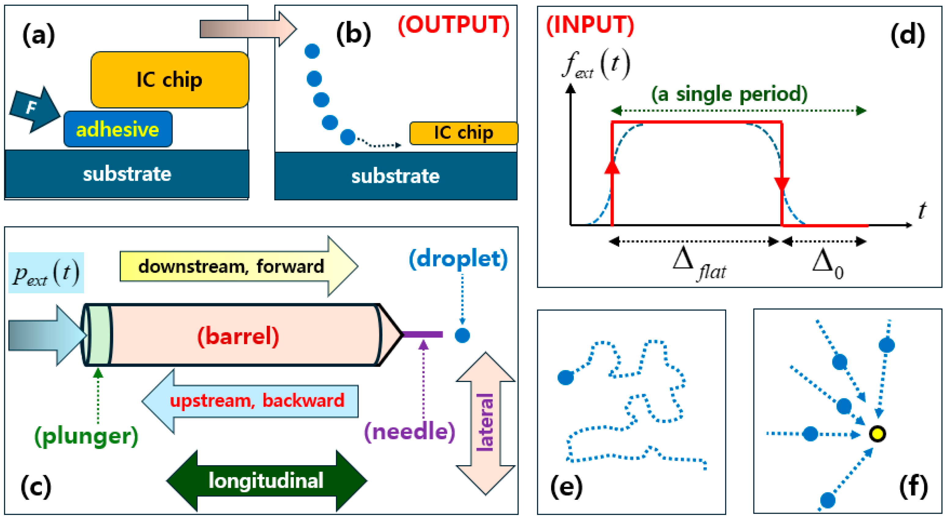
Figure 2.
(a) A string of finite length with both ends being held fixed for simplicity. (b), (c) and (d): Cylindrical hollow tubes of finite length with fluid filling the insides under higher internal pressures (namely, positive transmural pressures): (b) under steady state, (c) under transient state with decreasing axial pressure, and (d) under transient state with increasing axial pressure.
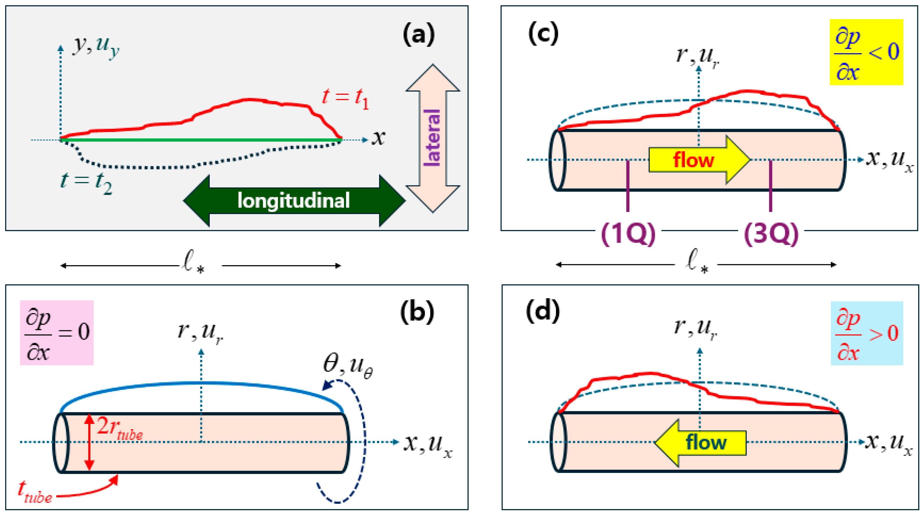
Figure 3.
(a) A segmented portion of a continuous four-component electric circuit. The given space is divided into a system and an environment or ambient. This continuous circuit is defined to be leak-free if , while it is defined to be leaky if and . (b) a full leaky RLGC circuit, (c) a leak-free RLC circuit, and (d) a rotation-free leaky RGC circuit.
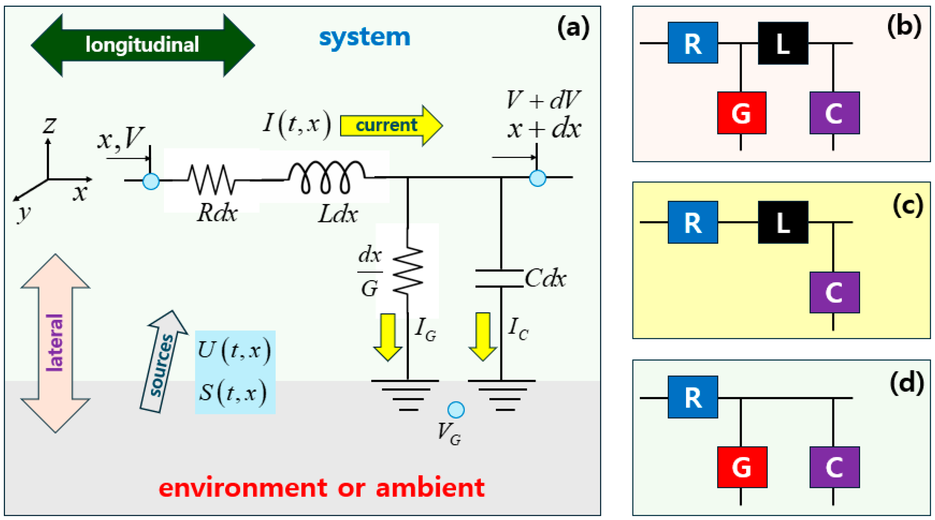
Figure 4.
and versus . The common horizontal coordinate is not to scale, where the numbers correspond respectively to in units of Hertz. Notice especially that in dimensional units as proved in Appendix A. All data is taken from [56], whence are expressed in the common MKS units. Therefore, the relative positions of the data on this Figure would have been uniformly shifted only in the vertical direction depending on the other units employed.
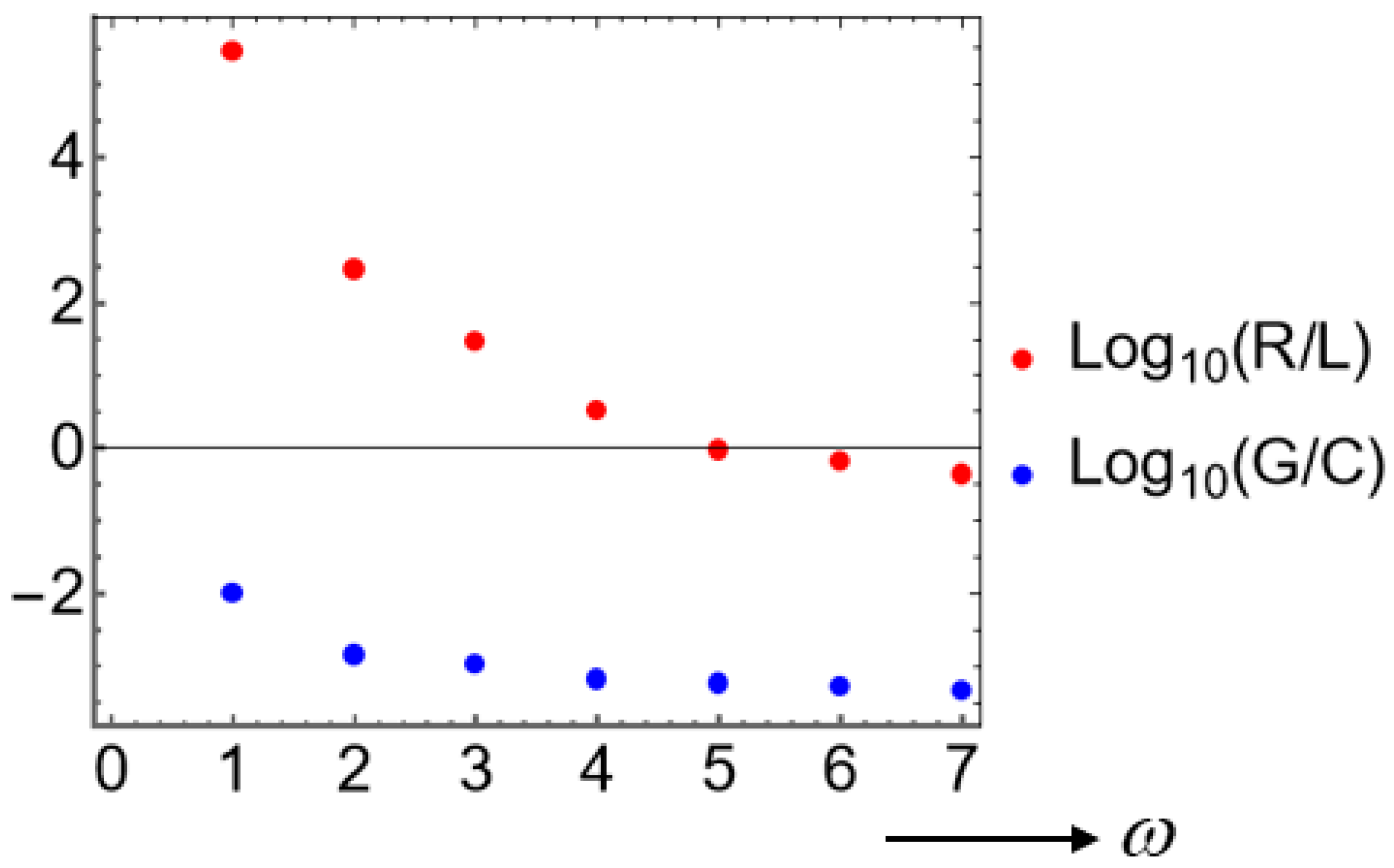
Figure 5.
Solid curves show the propagation constants and , while dashed curves display the attenuation rates and . Both and are obtained for the full leaky RLGC circuit, whereas both and are obtained for the leak-free RLC circuit. The horizontal axis is the dimensionless frequency and for the respective circuits. Three varying values of are assigned to different curves for both and . (a) a smaller display window. (b) a larger display window.
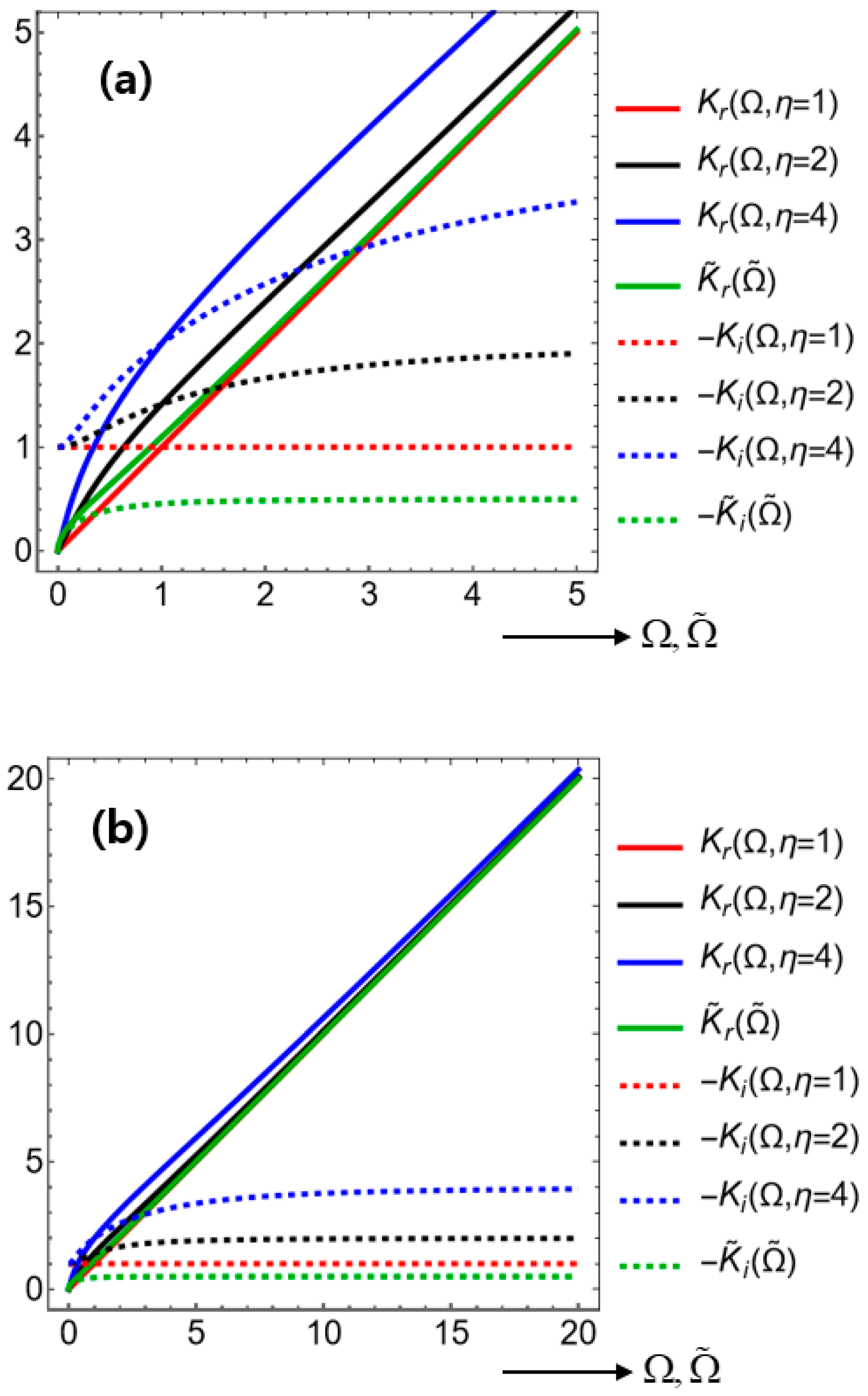
Figure 6.
Solid curves show the phase velocities and , while dashed curves display the group velocities and . Both and are obtained for the full leaky RLGC circuit, whereas both and are obtained for the leak-free RLC circuit. The horizontal axis is the dimensionless frequency and for the respective circuits. Three varying values of are assigned to different curves for both and. (a) a smaller display window. (b) a larger display window. This Figure is analogous to what is presented in [49].
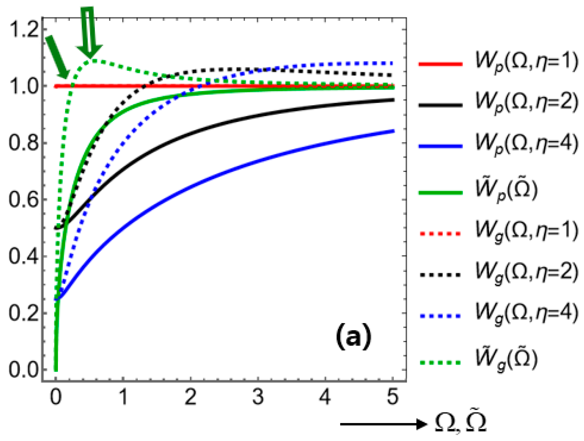
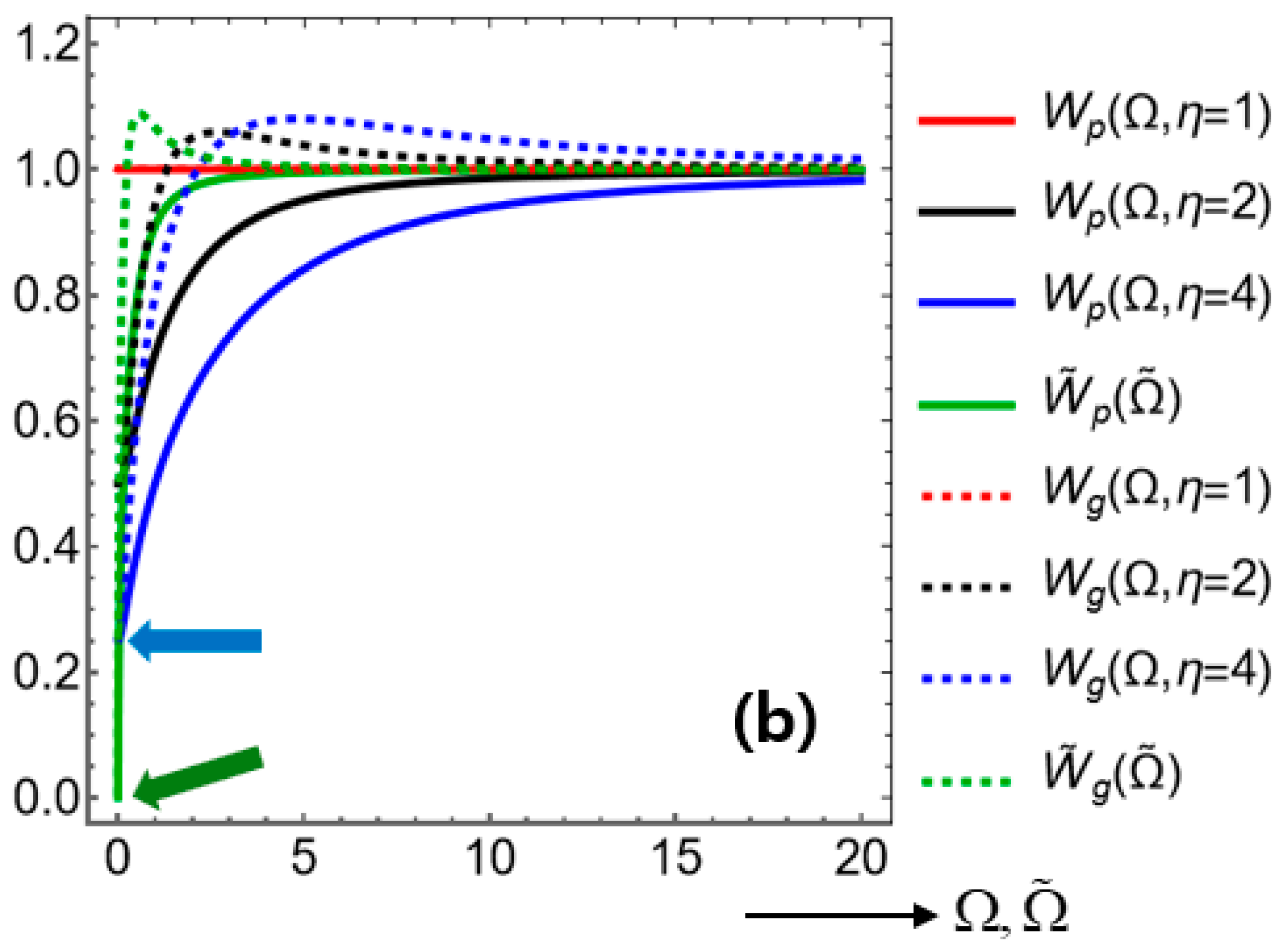
Figure 7.
Dispersion characteristics for the rotation-free leaky RGC circuit plotted against the dimensionless frequency . (a) The propagation constant on the solid red curve. (b) The attenuation rate on the dashed red curve. (c) The phase velocity on the solid black curve. (d) The phase velocity on the solid blue curve.
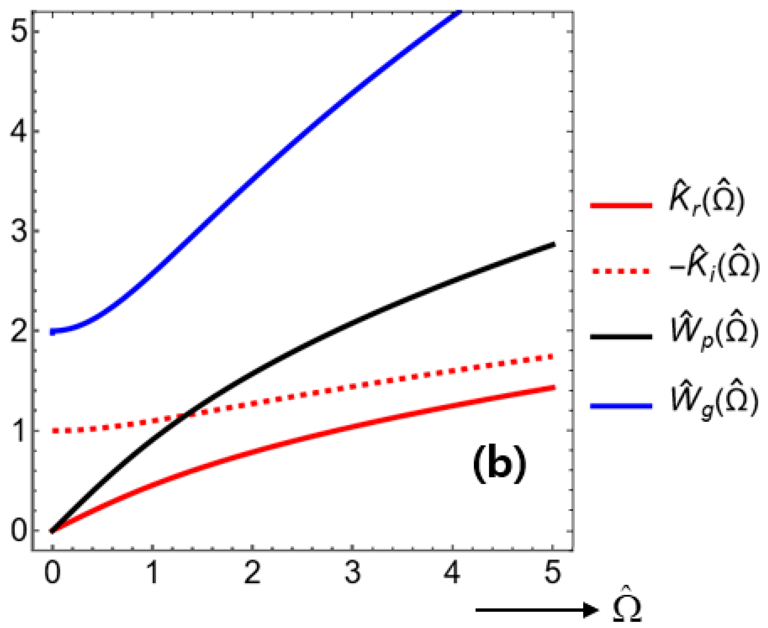
Figure 8.
A single discrete electric circuit with discrete four elements consisting of with . The system with is arranged in distinct ways: (a) serial, and (b) parallel, whereas the SEI elements remains in parallel to each other.
Figure 8.
A single discrete electric circuit with discrete four elements consisting of with . The system with is arranged in distinct ways: (a) serial, and (b) parallel, whereas the SEI elements remains in parallel to each other.
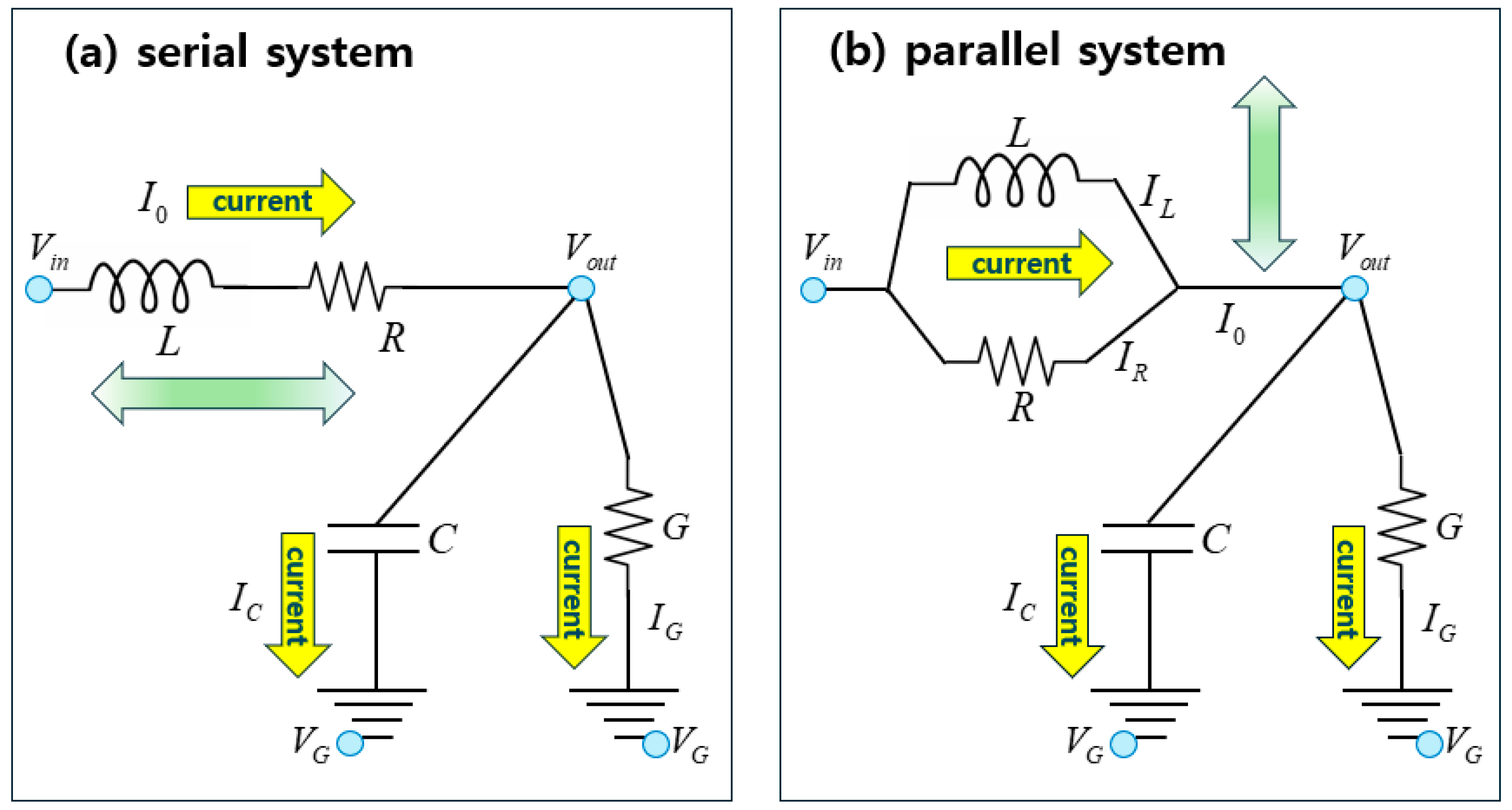
Figure 9.
The magnitudes of response functions plotted against the dimensionless frequency for varying values of . Each of is assigned to each subfigure.
Figure 9.
The magnitudes of response functions plotted against the dimensionless frequency for varying values of . Each of is assigned to each subfigure.
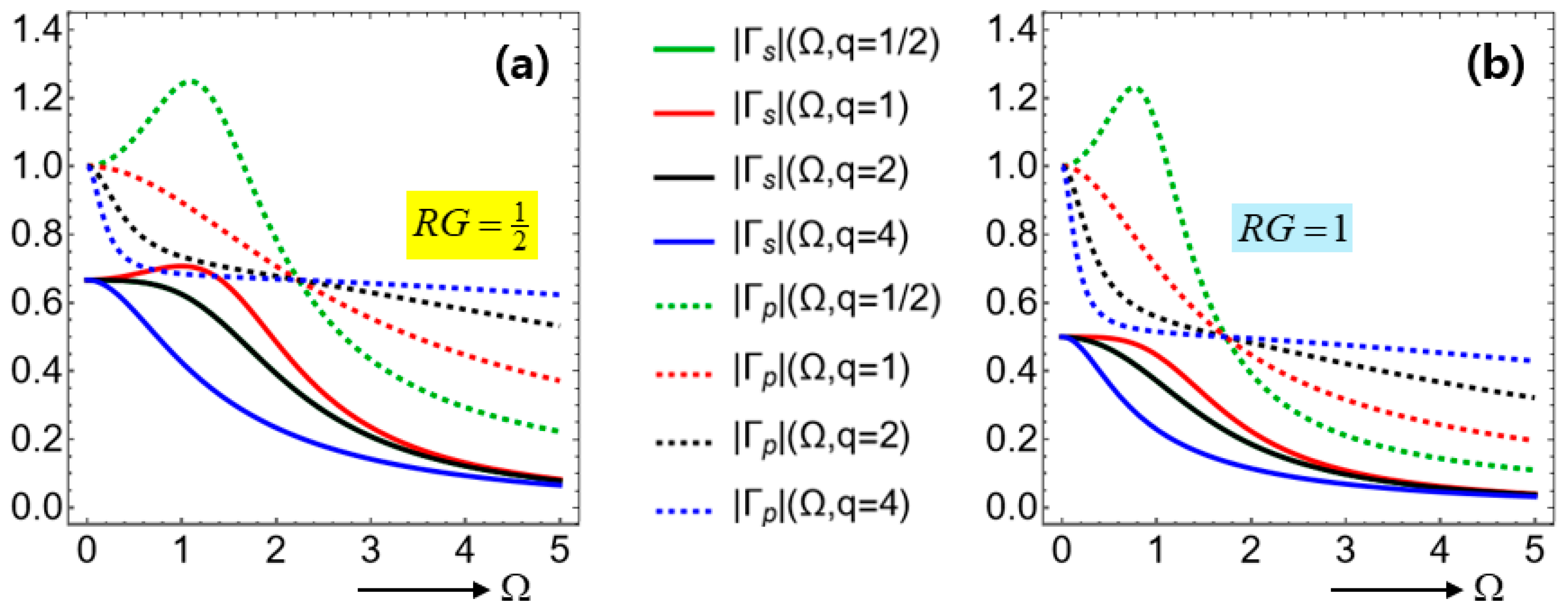
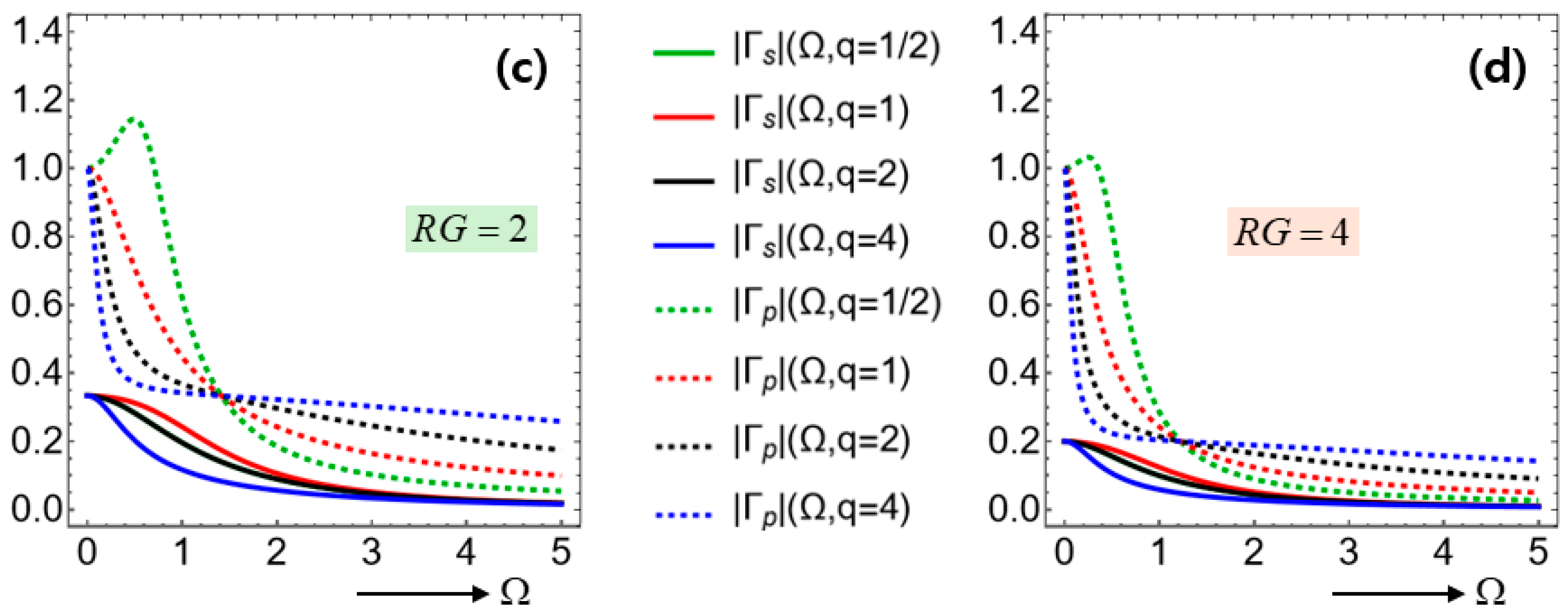
Figure 10.
The magnitudes of response function plotted against the dimensionless frequency for varying values of but for the same value of . Only parallel configuration is examined here for the system elements.
Figure 10.
The magnitudes of response function plotted against the dimensionless frequency for varying values of but for the same value of . Only parallel configuration is examined here for the system elements.
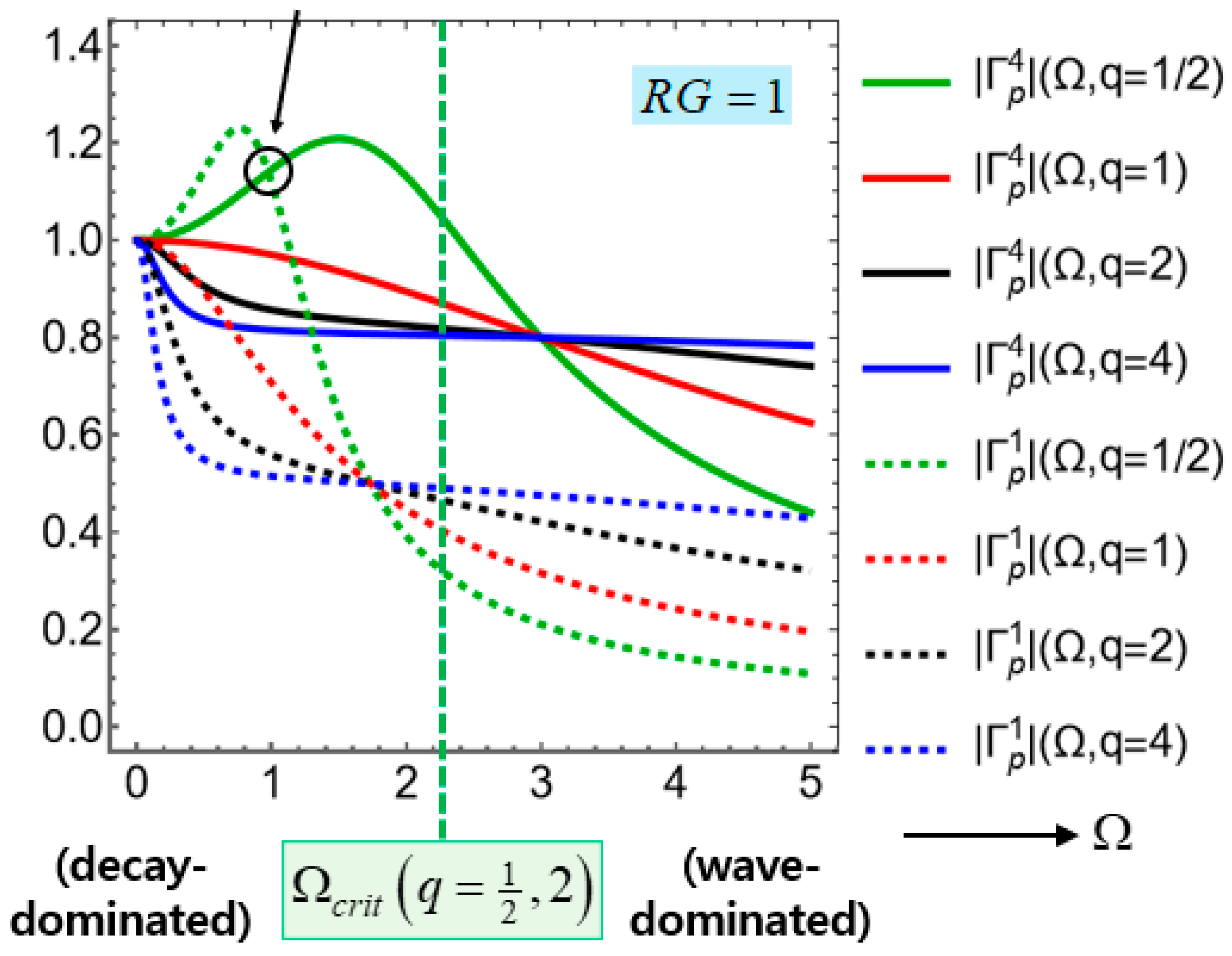
Table 1.
Comparison among various fluid-ejection devices
| Devices | droplets | dimension |
| medical syringe 1 | a single droplet | mostly 1-D |
| droplet dispenser 2,3 | train of droplets 2 | mostly 2-D |
| spiking neural network | multiple convergent trains of droplets | 3-D in general |
| 3-D bioprinter | a relatively continuous fluid ejection | mostly 1-D |
1 Both a dispenser for a cup of water and a dispenser for a cup of draft beer are operated in an analogous manner. 2 Inkjet printers for printing color agents on flat-panel displays work via analogous principle [7]. 3 The volume of each droplet is on the order of micro-liters in case with our droplet dispensers.
Table 2.
Fluid flows and longitudinal pressure gradients
| subfigure on Figure 2 | flow direction | pressure gradient | pressure transient |
| (b) | no flows | ||
| (c) | flows downstream | pressurization | |
| (d) | flows upstream | depressurization |
Table 3.
Dimensional features of resistance, capacitance, and inductance along with several of their combinations
Table 3.
Dimensional features of resistance, capacitance, and inductance along with several of their combinations
| symbol | name | dimension | temporal | interaction |
| resistance | 1-D (3-D) | static | system | |
| inductance | 3-D | dynamic | system | |
| capacitance | 2-D | dynamic | SEI1 | |
| conductance | 1-D (3-D) | static | SEI | |
| relative resistance | 3-D | static | system | |
| relative conductance | 2-D (3-D) | static | SEI1 | |
| effective stiffness | 1-D (3-D) | static | System-SEI | |
| effective mass | 3-D | dynamic | System-SEI | |
| membrane time | 2-D | dynamic | System-SEI | |
| system impedance | 3-D | dynamic | system | |
| SEI impedance | 2-D | dynamic | SEI |
1 SEI (system-environment interaction)
Table 4.
Reduced telegraph equations and component phenomena underlying the source-free telegraph equation (9)
Table 4.
Reduced telegraph equations and component phenomena underlying the source-free telegraph equation (9)
| key phenomena | reduced source-free equation with |
| telegraph equation for a full leaky circuit with | (9) 1 |
| diffusion-leak (or heat) equation with and | (20) |
| leak-free diffusion-wave equation with and | (18) |
| two equations defining temporal delay (decay) | (7) |
| harmonic oscillator | (17] |
1 This number indicates the equation number employed within this study
Table 5.
Comparison among the full leaky RLGC circuit with , the leak-free RLC circuit with and , and the rotation-free leaky circuit with and
Table 5.
Comparison among the full leaky RLGC circuit with , the leak-free RLC circuit with and , and the rotation-free leaky circuit with and
| Circuit type | Properties and reference times | dispersion characteristics |
| full leaky RLGC circuit on Figure 3(b) | (32)1 | (11), (31), (37) |
| Leak-free RLC circuit on Figure 3(c) | (34) | (33), (37) |
| Rotation-free leaky RGC circuit on Figure 3(d) | (45) | : square-root dispersion (44), (46) |
| Rotation-free and leak-free circuit | (49) | : square-root dispersion (49), (50) |
| resistance-conductance-free system | (16), (51) | : linear dispersion (51), (52) |
1 This number indicates the equation number employed within this study
Disclaimer/Publisher’s Note: The statements, opinions and data contained in all publications are solely those of the individual author(s) and contributor(s) and not of MDPI and/or the editor(s). MDPI and/or the editor(s) disclaim responsibility for any injury to people or property resulting from any ideas, methods, instructions or products referred to in the content. |
© 2025 by the authors. Licensee MDPI, Basel, Switzerland. This article is an open access article distributed under the terms and conditions of the Creative Commons Attribution (CC BY) license (http://creativecommons.org/licenses/by/4.0/).
Copyright: This open access article is published under a Creative Commons CC BY 4.0 license, which permit the free download, distribution, and reuse, provided that the author and preprint are cited in any reuse.


