Submitted:
04 December 2025
Posted:
09 December 2025
You are already at the latest version
Abstract
We present a comprehensive and automated methodology for processing two-dimensional X-ray diffraction (2D-XRD) patterns. The proposed workflow involves three sequential stages: (i) precise localization of the diffraction center, (ii) removal of high-frequency noise, and (iii) suppression of non-physical background signals. This method enables improved data quality for subsequent quantitative analysis such as radial integration, phase identification, and structural refinement. Application to experimental datasets from both the Synchrotron Radiation Facility and a table-top X-ray diffractometer demonstrates the method’s robustness, accuracy, and computational efficiency.
Keywords:
X-ray diffraction
; image processing
; center localization
; background suppression
; denoising
1. Introduction
The use of two-dimensional (2D) area detectors in synchrotron and laboratory-based X-ray diffraction (XRD) experiments has become increasingly widespread, driven by the availability of fast and high-efficiency detectors. Consequently, the volume and rate of data acquisition have increased substantially, particularly in time-resolved studies of dynamic processes such as phase transitions, melting and chemical reactions. Real-time data analysis is therefore essential for interpreting sample behaviour and for adjusting experimental parameters during acquisition.
Despite the availability of established software such as Fit2D [1], existing tools often exhibit limitations in processing speed, calibration flexibility and user interaction. Fit2D, though long regarded as a standard in the field, suffers from an outdated interface, slow image integration and challenges in calibrating complex detector geometries, particularly when the beam centre lies outside the image or the detector is strongly tilted. These issues can restrict the design and flexibility of XRD experiments, especially under demanding conditions such as high pressure or temperature.
To overcome these limitations, modern software platforms have been developed for rapid, interactive and versatile 2D XRD data processing—such as Dioptas [2]—often implemented in Python and based on a modular Model–View–Controller (MVC) architecture. These tools achieve high computational performance while maintaining extensibility and ease of use. Core tasks, including integration, calibration and visualisation, are accelerated through established scientific libraries (e.g. NumPy, SciPy, pyFAI) [3,4], while graphical interfaces enable fast rendering and intuitive data exploration.
While computational speed and automation represent major advances, the development of analytically rigorous and statistically robust routines is equally critical for quantitative accuracy and reproducibility. Rather than focusing solely on optimisation of existing algorithms, the present work introduces new mathematical and statistical methods designed to enhance the reliability of key analytical steps, including centre identification, background estimation and calibration refinement. Such approaches enable automated yet interpretable data evaluation, even in the presence of noise, overlapping reflections or incomplete detector coverage.
Combining high computational efficiency with mathematically grounded analysis establishes a comprehensive framework for accurate and reproducible 2D XRD data processing. The integration of speed, interactivity and statistical rigour enhances both the practical efficiency and scientific reliability of modern diffraction analysis. The present paper focuses primarily on the mathematical aspects rather than on computational or visualisation tasks, and is not intended as a review or promotion of existing software, although comparison with at least one available package is included for validation.
2. Centre Localization
2.1. User-Supervised Aspects of Centre Localization in the Calibration Procedure
The process of centre localization constitutes one of the most user-sensitive stages of the calibration procedure. Although the implemented workflow is generally comprehensive and adaptable, it still depends strongly on user supervision at several points. In particular, the initialization of the calibration relies on user-supplied parameters such as approximate beam centre coordinates, detector distance, and orientation. Any inaccuracy in these preliminary entries can propagate through the subsequent steps, thereby compromising the overall calibration quality.
In situations where automatic algorithms fail to converge or misidentify the diffraction centre—often due to low image contrast, incomplete ring patterns, or high noise levels—manual intervention becomes essential. Users are typically required to manually adjust the estimated centre or select specific diffraction rings/peaks for guidance. This introduces a degree of subjectivity and demands a certain level of expertise, since the visual assessment of whether the rings appear concentric or whether cake lines are straight serves as the primary qualitative verification method. Such inspection-based validation, while practical, is inherently prone to interpretation errors and lacks quantitative robustness.
Automation, although available, is not fully reliable. The automatic centre-finding routines may require user supervision, such as toggling between single-ring and multi-ring/peak detection or refining the selection of regions of interest. The sensitivity of the localization process to data quality further limits its autonomy: when dealing with weak or incomplete diffraction patterns, users often need to adjust thresholds or apply spatial masks to constrain the fit. The effectiveness of these manual corrections, however, depends on the user’s experience and understanding of the image features.
The absence of diagnostic feedback mechanisms compounds these challenges. When centre localization fails to yield consistent results, the current approach generally resorts to a trial-and-error exploration of parameter combinations, which can be time-consuming and inefficient. Moreover, the system does not provide clear indications of the cause of failure—whether stemming from poor data quality, misestimated input parameters, or algorithmic limitations—thus placing the diagnostic burden entirely on the user.
Finally, reproducibility remains an issue. Since manual centre adjustments and ring selections vary from one operator to another, the resulting calibrations may differ slightly across users. Additionally, the lack of automated logging means that user actions and parameter settings during the centre localization step are not systematically recorded, hindering the ability to reproduce or audit previous calibration sessions. Consequently, while the procedure enables flexible and accurate centre determination, it still relies heavily on informed user participation to ensure both reliability and reproducibility.
For instance, the results of applying the same Dioptas unsupervised calibration routine to identical diffraction datasets are shown in Figure 1. These include patterns collected at the Synchrotron Radiation Facility (S04387, top row), which are affected by experimental setup artefacts and exhibit additional noise, shadows, and generally poor data quality, as well as patterns acquired using a table-top X-ray diffractometer (152762, bottom row), characterised by low counting statistics. The four panels illustrate how the routine may yield different ring selections (red markers), leading to variability in centre localisation and profile extraction, whereas user-supervised intervention (single-peak search) ensures consistent ring detection.
2.2. Unsupervised Centre Localization
Unlike several existing approaches—including radial symmetry analysis and ring fitting [5]—that optimise the beam centre with subpixel accuracy, the sniper2D function developed in this study provides a novel, unsupervised algorithm for centre localisation in two-dimensional images, such as X-ray diffraction (XRD) patterns, based on correlation analysis. The algorithm identifies the horizontal and vertical center of an image by correlating it with its shifted versions and selecting the shifts that result in the highest correlation. The result is a set of coordinates [xc, yc] that represent the center of the image. Here is a breakdown of what the algorithm does (see the supplementary material for the full algorithm):
- 1. Image Preparation: imgLR (resp. imgUD) is the horizontally (resp. vertically) flipped version of the image.
- 2. Variable Initialization: ny, nx store the height and width of the input image. cx, cy are initialized to zero and will store the maximum correlation values for the x and y directions. sx, sy are initialized to zero and will be used to iterate through shifts in the x and y directions.
- 3. Horizontal Search (X-axis): the algorithm performs a search for the center of the image along the x-axis using sx, which is incremented starting from 0. It creates two shifted versions of the horizontally flipped image (auxp and auxm) using positive and negative shifts by sx. It computes the correlation between the original image and these shifted versions (auxp, auxm), and updates the center xc and the maximum correlation value cx if the correlation exceeds previous values. This process continues until sx exceeds nx/8.
- 4. Vertical Search (Y-axis): the same process is repeated for the y-axis, where sy iterates over vertical shifts. It computes auxp and auxm for the vertically flipped image (imgUD) and performs the same correlation comparison to find the vertical center yc and the maximum correlation value cy.
- 5. Output: the final output is the coordinates [xc, yc], representing the center of the image or the location of the peak feature based on correlation.
In the analysis of X-ray diffraction (XRD) two-dimensional (2D) patterns, enhancing the information content of the measured intensity distribution can significantly improve the accuracy of centre localisation. To this end, we apply a theorem demonstrating that a scale-free, uncorrelated modulation of a normalized positive function can reduce its entropy. In practice, this principle is employed to preprocess an XRD 2D pattern prior to applying the centre localization algorithm (sniper2D). By selectively concentrating probability mass, the modulation increases structural contrast and lowers the pattern’s entropy, thereby enabling more accurate and robust localisation of the diffraction centre.
The modulation is realised through a scale-free function defined as
which depends solely on the local angular variations of the intensity field and is independent of its absolute scaling. Although is ideally1 uncorrelated with , their interaction through the modulated field
where denotes a scaling factor, redistributes the probability density in a manner that selectively emphasises spatial features associated with meaningful structural variations. This process effectively compresses redundant information while amplifying directional gradients that encode the intrinsic geometry of the diffraction pattern.
The entropy reduction ensured by the theorem is therefore not merely a mathematical artefact of normalization but reflects a genuine improvement in the organisation of information. For diffraction analysis, this results in a clearer and more interpretable 2D pattern from which the sniper2D algorithm can extract the diffraction centre with greater precision and stability. The scale-free nature of ensures that this enhancement is robust to intensity scaling, making the approach particularly suitable for experimental data characterised by broad dynamic ranges or nonuniform exposure.
For completeness, a formal proof of the theorem is outlined in the Appendix A.1.
The results are shown in Figure 2, where the centres estimated by the sniper2D algorithm using intensity or intensity–phase data are juxtaposed with the corresponding 2D diffraction patterns. These include patterns collected at the Synchrotron Radiation Facility (S04388, affected by experimental setup artefacts, and S04387, exhibiting additional noise, shadows, and poor data quality) and at a table-top X-ray diffractometer (152762, with low counting statistics, and resummed, with higher counting statistics). Quantitative metrics for the diffraction ring analysis and ring centres compared with Dioptas, are reported in Table 1 for a scaling factor .
3. Denoising
A recent study [6] introduced the Lattice Boltzmann Method (LBM) [7,8,9] as an innovative approach to enhance the quality of two-dimensional X-ray diffraction (XRD) patterns. XRD is a key technique in materials science and crystallography for determining atomic structures, yet its effectiveness is often limited by the presence of noise that obscures subtle but critical features. Traditional denoising techniques typically struggle to preserve the fine details of diffraction data, motivating the use of alternative numerical models. In this context, LBM, originally developed for simulating fluid dynamics on discrete lattices, is adapted to model diffusion processes in XRD images by treating the signal and noise as distinct interacting components. Through the simulation of diffusion dynamics, the method efficiently separates noise from the true diffraction signal, producing cleaner and more accurate data. Tests reported in the original work demonstrated substantial improvements in signal-to-noise ratio and robustness against Poissonian noise, while maintaining the fidelity of structural features. Owing to its numerical stability, efficiency, and feature-preserving properties, LBM represents a valuable tool for improving XRD data interpretation. In the present work, this method is employed with the same parameter settings described in [6] to process comparable two-dimensional diffraction patterns.
The algorithm implements a two-dimensional nine-velocity (D2Q9) Lattice Boltzmann scheme for denoising two-dimensional patterns, following the Bhatnagar–Gross–Krook (BGK) approximation [10]. The parameters , , and define the relaxation rate (), while the discrete velocity set and corresponding weights define the D2Q9 lattice.
The equilibrium distribution is initialized from (being I the original image2) and weighted by W, while N is randomly initialized. At each time step, the streaming step propagates along using periodic boundary conditions. The macroscopic fields are updated as and from the equilibrium moments. A discretized Maxwell–Boltzmann equilibrium function, denoted , is constructed as
In the collision step, the algorithm computes local gradients and a scale parameter , then derives adaptive weights . The weighted divergence term is used to relax the system:
After iterations, the reconstructed (denoised) density field is computed as
This process iteratively separates signal from noise while preserving structural details in the input pattern.
A schematic outline of the implemented algorithm is provided in the Appendix A.2 for reference.
For the denoising procedure, a direct comparison with an alternative method has been omitted, as the original manuscript [6] provides a detailed analysis of this aspect. Interested readers are referred to this work for further details.
4. Background Suppression
4.1. User-Dependent Aspects in Background Subtraction within the Integration Procedure
The background subtraction stage of the integration procedure remains highly user-dependent. Sternberg’s 1983 work [12] introduced the rolling-ball algorithm, modelling images as three-dimensional intensity surfaces and estimating the background via a simulated rolling sphere. This elegant and robust method became foundational in microscopy and biomedical imaging, and is widely adopted in software such as ImageJ [13,14].
Although these methods offer flexibility, they require substantial manual tuning of parameters such as smoothing width, iteration number, and polynomial order, guided primarily by visual inspection and prior experience. This introduces variability and limits quantitative assessment, as objective measures of fit quality are generally absent.
Selection of the region of interest for fitting adds further user dependence. Inaccurate choices can include noise or omit relevant intensity features, distorting the integrated profile. Consequently, visual comparison between original and background-subtracted patterns remains the principal, though subjective, validation approach, especially in noisy or complex diffraction data.
Algorithm parameters, such as the interplay between smoothing width and polynomial order, are often opaque, risking over- or underfitting. The absence of warnings or safeguards allows distortions or unrealistic background shapes to go unnoticed. Moreover, parameter values are not automatically logged, hindering reproducibility; different users may obtain divergent results from the same dataset.
The integration stage, including tools such as supersampling, also demands caution. Supersampling can enhance resolution and smoothness but may generate artefacts if misapplied, and no quantitative diagnostics or automated checks exist. The lack of preview or undo functionality further limits reversibility.
In summary, background subtraction within the integration workflow remains a user-sensitive process requiring careful parameter tuning, informed judgment, and systematic record-keeping. Enhanced guidance, quantitative feedback, and automated safeguards would improve robustness and reproducibility.
4.2. Data-Driven Background Estimate
In the current work, we begin by considering an intensity measurement that is composed of two unknown or blind contributions: a slowly varying background and a localized signal . In other words, the observed intensity at each point is the sum of these two components, whose individual shapes are not known a priori.
Now consider the perturbed intensity product
where the represent small random shifts along the radial coordinate. Physically, this models multiple measurements in which the underlying background is nearly constant, while the localized signal features are narrow and randomly displaced.
Because the background changes only slowly with r, it can be treated as essentially constant over each perturbation. The localized signals are sparse and do not significantly overlap, so their contributions remain limited. As a result, when taking the product over many measurements, the relative influence of the signals diminishes compared to the background.
Mathematically, factoring out the background from the product and bounding the residual signal terms yields
As the number of measurements n increases, both and the term involving the maximum signal contribution approach 1, leading to the convergence
In practical terms, this shows that taking the geometric mean of multiple perturbed intensity measurements effectively isolates the background, washing out the localized signals and revealing the slowly varying component as the dominant contribution.
For completeness, a formal proof of the theorem is outlined in the Appendix A.3.
The results are shown in Figure 3 and Figure 4, where the 2D backgrounds estimated by the present algorithm are compared with the corresponding 2D patterns computed by ImageJ for three choices of the rolling-ball radius (25/50/100 pixels). These include a pattern collected at the Synchrotron Radiation Facility (S04387, affected by experimental setup artefacts and exhibiting additional noise, shadows, and poor data quality), and another one collected at a table-top X-ray diffractometer (sam4). A comparison among the corresponding 1D semilogarithmic profiles is shown in Figure 5.
Quantitative metrics for the comparison of the same samples with ImageJ are reported in Table 2. The apparent discrepancy between 2D Pearson’s correlation coefficient and the 2D Structural Similarity Index (SSIM) [15] for the S04387 sample backgrounds is explained as follows. A high correlation reflects a strong linear relationship but does not guarantee a high SSIM, which also takes into account perceptual factors such as luminance, contrast, and texture. Thus, the patterns may share similar global intensity variations but differ in local structure, leading to high correlation and lower SSIM. This highlights the need to consider both metrics in image analysis.
The metrics reported in Table 2 indicate a generally strong agreement between the background estimations produced in the present work and those obtained using ImageJ across a range of rolling–ball radii. For sample S04387, the background constitutes only a small fraction of the overall signal (3%), and the correlation with the ImageJ backgrounds remains consistently high (approximately 0.9) regardless of radius. However, the SSIM values are more modest (around 0.55), suggesting that although the global trends are well captured, finer structural details differ to a greater extent. The residuals are correspondingly small, remaining close to 1% of the total intensity.
In contrast, sample sam4 exhibits a substantially larger background contribution (59%), and here both the correlation and SSIM values indicate an excellent match to the ImageJ estimates, particularly for radii of 50–100 pixels (Corr ; SSIM ). The residuals decrease markedly with increasing radius, falling from 0.25 at 25 pixels to around 0.10 at 100 pixels, implying that larger radii provide a closer approximation to the background retrieved by the present method. Collectively, these results demonstrate that the proposed background–recovery approach performs robustly and is broadly consistent with established methods, with the level of agreement improving for samples with more substantial background structure.
5. Results
To evaluate the robustness of the proposed denoising approach under realistic experimental conditions, the model was applied to X-ray diffraction (XRD) patterns obtained from tendon-derived collagen molecules (rat tail in this paper). Under varying biochemical environments, these molecules self-assemble into a hierarchical superstructure of triple helices, exhibiting a pronounced preferred orientation. This orientational order is evident in the -symmetric partial arcs observed in Figure 6, Figure 7-left and Figure 8-top-left, which replace the fully 2-symmetric diffraction rings typically associated with isotropic samples. Such superstructural organization, together with the high degree of crystallinity within the fibrillar domains, contributes significantly to the mechanical stiffness of the tissue (for details of sample preparation and experimental procedures, see [16]). Figure 6 compares the corresponding XRD patterns: the original dataset (top left panel) was acquired over an integration time of 2400 , yielding a maximum count below 1000.
For the sake of completeness, two additional figures are presented in Figure 9: 1D semilogarithmic profiles obtained using the present approach (right) and 2D original maps (left) for the rat tail sample, acquired at varying exposure times: 171568 s (centre) and 327350 s (bottom), yielding a maximum count around 60000, along with the analogous profiles obtained using Dioptas for reference.
Small-angle and wide-angle X-ray scattering (SAXS/WAXS) measurements were performed at the X-ray Micro Imaging Laboratory (XMI-LAB [17]) on both raw collagen flakes and processed collagen films. The experimental setup comprised a Fr-E+ SuperBright rotating Cu anode microsource () equipped with Confocal Max-Flux optics and a SAXS/WAXS three-pinhole camera. WAXS data were recorded on a 250 × 160 image plate detector (pixel size 100 ) and read using an off-line RAXIA system. Each sample was mounted on a fixed holder, and data were collected from three distinct positions. The incident beam spot size was approximately 200 , with a sample-to-detector distance of 10 , providing a scattering vector (q) range of 3/–35/, corresponding to d-spacings of 0.18–2.5.
The X-ray diffraction images 152762 and resummed in Figure 2 (bottom panels) correspond to vesicle-in-gel samples also measured on the diffractometer at the XMI-LAB [18]: the diffraction pattern 152762, with an acquisition time of 45 seconds, exhibits a ring of very low intensity in Figure 2 (bottom left), which is nonetheless discernible in the 1D radial integration plot, where a peak appears at approximately . The pattern obtained by summing all acquisitions of the sample clearly highlights the presence of the aforementioned ring (resummed) in Figure 2 (bottom right).
Another example of wide-angle X-ray diffraction (WAXD) fibre-pattern denoising is provided by the linen samples characterized in [19]. The specimens (sam4 in this paper) consisted of threads approximately 1 in length and 0.2–0.6 in width. WAXS measurements were performed on all linen samples at the X-ray Micro Imaging Laboratory (XMI-LAB) using an experimental setup similar to that described above, equipped additionally with an X-ray scanning microscope. Data were collected on an image plate (IP) detector and read off-line using a Rigaku RAXIA-Di system. Each linen thread, mounted directly on the sample holder, was exposed for 1800 . The incident beam spot size at the sample position was approximately 200 , and the image plate detector was positioned at a distance of 10 . This geometry provided access to scattering vector magnitudes defined as
where is half the scattering angle, i.e., the angle between the incoming beam and the detector direction and is the wavelength of the incident radiation. It covers a range from approximately 1.5/−1 to 35/−1. Following geometric calibration, the two-dimensional (2D) diffraction images were azimuthally integrated to yield one-dimensional (1D) intensity profiles. Further details of the experimental configuration and data analysis procedures can be found in the original publication. The outcome of the image processing algorithm is presented in Figure 7-right, Figure 8-top-right and Figure 10.
The algorithm scheme can also be fruitfully applied to the XRD patterns collected at the Synchrotron Radiation Facilities (namely S04387 and S04388 patterns in Figure 2-top). The Pilatus II is a single photon counting pixel detector, e.g. used at the PSI Facility [20], renowned for its high spatial resolution and efficiency in detecting low-intensity X-ray beams. It features an advanced hybrid pixel array that counts individual photons, offering exceptional precision and dynamic range. This detector is pivotal for experiments requiring detailed imaging and analysis, such as those in structural biology and materials science. Its performance is enhanced by its low noise and high count rate capabilities, making it a versatile tool for cutting-edge research in various scientific fields. However, low statistics two-dimensional images, sometimes affected by artefacts (e.g. experimental setup shadows), could benefit from a pre-processing denoising: in Figure 2-top the application of the sniper2D algorithm is illustrated in such a case, while the result of the entire image processing is shown in Figure 8 (bottom panels, Figure 11 and Figure 12).
These issues have collectively met the need for better automation, real-time validation, and user guidance to reduce the burden and risk of incorrect user supervision. The application of the sniper2D algorithm to all aforementioned 2D XRD patterns is summarised in Table 1, which also provides a numerical comparison with the results obtained using the Dioptas software. The corresponding one-dimensional semilogarithmic profiles are presented in Figure 8.
The metrics summarised in Table 1 provide an overview of the information content and angular–intensity relationships present in the diffraction images, together with a comparison of ring centre positions determined in the present work against those obtained using Dioptas. The intensity entropy values span a broad range, reflecting differing levels of structural complexity across the samples: sam4 and the long-exposure rat-tail datasets exhibit relatively high entropy (around 0.30–0.35), whereas sample 152762 shows very low entropy (0.01), consistent with a markedly simpler intensity field.
A key observation is that the entropy computed on the joint distribution is systematically lower than the entropy of the intensity pattern alone for every sample. This reduction is expected, as conditioning on the angular variable restricts the available variability within the data, thereby lowering the overall information content of the resulting distribution. The consistent decrease across all entries supports the interpretation that the angular dependence introduces additional structure rather than additional randomness.
The correlations between the intensity gradients and the azimuthal angle are generally weak and hover close to zero, indicating that directional variations in intensity are not strongly aligned with the angular coordinate. This behaviour is compatible with the moderate joint entropy values, which reflect increased structural organisation in more complex patterns.
Finally, the comparison of ring centres reveals good agreement between the two methods: for most samples, the centre coordinates determined here differ from the Dioptas values by only a few pixels. The rat-tail datasets show the largest offsets (up to roughly 10 pixels), whereas samples such as S04387, sam4, and 152762 exhibit close numerical correspondence. Overall, these results demonstrate that the present analysis method provides centre estimates consistent with established software while offering additional quantitative insight through entropy-based characterisation of diffraction-pattern structure.
6. Conclusions
The calibration system presented in this work minimises reliance on user expertise, judgement, and trial-and-error, reducing inconsistency and inefficiency. By automating common failure recovery, providing real-time quality metrics, and offering clearer guidance, the workflow requires less direct supervision while maintaining high accuracy and computational efficiency. Application to both synchrotron and laboratory XRD datasets demonstrates its robustness and versatility, facilitating reliable quantitative analysis. This automated methodology has the potential to streamline routine 2D XRD processing and improve reproducibility in structural characterisation studies.
Author Contributions
For research articles with several authors, a short paragraph specifying their individual contributions must be provided. The following statements should be used “Conceptualization, X.X. and Y.Y.; methodology, X.X.; software, X.X.; validation, X.X., Y.Y. and Z.Z.; formal analysis, X.X.; investigation, X.X.; resources, X.X.; data curation, X.X.; writing—original draft preparation, X.X.; writing—review and editing, X.X.; visualization, X.X.; supervision, X.X.; project administration, X.X.; funding acquisition, Y.Y. All authors have read and agreed to the published version of the manuscript.”, please turn to the CRediT taxonomy for the term explanation. Authorship must be limited to those who have contributed substantially to the work reported.
Funding
This research received no external funding.
Institutional Review Board Statement
In this section, you should add the Institutional Review Board Statement and approval number, if relevant to your study. You might choose to exclude this statement if the study did not require ethical approval. Please note that the Editorial Office might ask you for further information. Please add “The study was conducted in accordance with the Declaration of Helsinki, and approved by the Institutional Review Board (or Ethics Committee) of NAME OF INSTITUTE (protocol code XXX and date of approval).” for studies involving humans. OR “The animal study protocol was approved by the Institutional Review Board (or Ethics Committee) of NAME OF INSTITUTE (protocol code XXX and date of approval).” for studies involving animals. OR “Ethical review and approval were waived for this study due to REASON (please provide a detailed justification).” OR “Not applicable” for studies not involving humans or animals.
Informed Consent Statement
Any research article describing a study involving humans should contain this statement. Please add “Informed consent was obtained from all subjects involved in the study.” OR “Patient consent was waived due to REASON (please provide a detailed justification).” OR “Not applicable” for studies not involving humans. You might also choose to exclude this statement if the study did not involve humans.
Written informed consent for publication must be obtained from participating patients who can be identified (including by the patients themselves). Please state “Written informed consent has been obtained from the patient(s) to publish this paper” if applicable.
Data Availability Statement
The MatLab code and XRD patterns are available.
Acknowledgments
The author wishes to acknowledge D. Altamura, T. Sibillano, and C. Giannini for providing him with XRD patterns.
Conflicts of Interest
The author declares no conflict of interest.
Appendix A. Supplementary Methods
Appendix A.1. Center Localization
Theorem
(Entropy Reduction via Uncorrelated Scale-Free Modulation). Let be a positive definite function over a domain , normalized such that . Let be a scale-free, positive definite function over the same domain, also satisfying . Assume:
- is computed based on but is scale-free, i.e., independent of the magnitude scaling of ρ;
- ρ and h are uncorrelated in the sense that:
- Let for some .
Then there exists a scale factor such that the entropy of the modulated function
is strictly smaller than the entropy of the unmodulated, scaled function:
where entropy is defined (up to a constant) as:
Proof
(Proof).
- (1)
- Normalization: Since both and h are normalized to have unit maximum, their product remains bounded by . Hence, entropy is well-defined for finite domains and positive definite functions.
- (2)
-
Entropy decomposition: Consider the entropy difference:This simplifies to:
- (2)
- Effect of : Because and is uncorrelated with , the last integral is positive.
- (2)
- Existence of optimal s: For large enough s, both terms are dominated by the scaling factors. However, since is subleading with respect to , there exists a threshold beyond which the entropy of remains strictly below that of .
- (2)
- Conclusion: Therefore, such a scale s exists.
□
Remark.
The key insight is that even though is scale-free and uncorrelated with , its interaction with the scaled ρ selectively reduces entropy by concentrating probability mass, a form of information compression.
Appendix A.2. Denoising
| Algorithm D2Q9 Lattice Boltzmann Simulation with Adaptive Relaxation |
|
Appendix A.3. Background Suppression
Theorem
(Asymptotic Dominance of Background in Perturbed Intensity Product). Let the perturbed intensity product in polar coordinates be given by
where:
- is the background function, assumed to be slowly varying in r,
- is a localized signal function,
- are random perturbations along the r-coordinate, intermediate in scale between the widths of s and b.
Then under the assumptions below, the geometric mean of converges to the background as :
Proof.
By the slow variation of the background, we approximate:
Factoring out the constant background term:
Assume that the signal contributions are localized and non-overlapping, i.e.,
Then applying the first-order product approximation:
we obtain:
Bounding the sum using , we get:
Thus, we establish the bounds:
Taking n-th roots and analyzing the limit:
Now use standard asymptotic results:
- ,
- ,
to conclude:
□
Assumption
(Summary of Key Conditions).
- The background is slowly varying: ,
- Signal overlaps are negligible: ,
- Signal values are bounded: ,
- Asymptotic properties: , as .
This shows that the background dominates the product asymptotically, and the geometric mean of the product converges to .
References
- Hammersley, A.P.; Svensson, S.O.; Hanfland, M.; Fitch, A.N.; Hausermann, D. Two-dimensional detector software: From real detector to idealised image or two-theta scan. High Pressure Res. 1996, 14, 235–248. [Google Scholar] [CrossRef]
- Prescher, C.; Prakapenka, V.B. DIOPTAS: a program for reduction of two-dimensional X-ray diffraction data and data exploration. High Pressure Res. 2015, 35, 223–230. [Google Scholar] [CrossRef]
- Kieffer, J.; Karkoulis, D. PyFAI, a versatile library for azimuthal regrouping. J. Phys.: Conf. Ser. 2013, 425, 202012. [Google Scholar] [CrossRef]
- Kieffer, J. PyFAI Documentation, 2024. Available online: https://pyfai.readthedocs.io.
- Loy, G.; Zelinsky, A. Fast radial symmetry for detecting points of interest. IEEE Trans. Pattern Anal. Mach. Intell. 2003, 25, 959–973. [Google Scholar] [CrossRef]
- Ladisa, M. Denoising X-Ray Diffraction Two-Dimensional Patterns with Lattice Boltzmann Method. Crystals 2025, 15, 51. [Google Scholar] [CrossRef]
- Chen, H.; Chen, S.; Matthaeus, W.H. Recovery of the Navier–Stokes equations using a lattice-gas Boltzmann method. Phys. Rev. A 1992, 45, R5339. [Google Scholar] [CrossRef] [PubMed]
- He, X.; Luo, L.S. Lattice Boltzmann Model for the Incompressible Navier–Stokes Equation. J. Stat. Phys. 1997, 88, 927–944. [Google Scholar] [CrossRef]
- He, X.; Luo, L.S. A priori derivation of the lattice Boltzmann equation. Phys. Rev. E 1997, 55, R6333. [Google Scholar] [CrossRef]
- Bhatnagar, P.; Gross, E.; Krook, M. A model for collision processes in gases. I. Small amplitude processes in charged and neutral one-component systems. Phys. Rev. 1954, 94, 511–525. [Google Scholar] [CrossRef]
- Mighell, K. J. Parameter Estimation in Astronomy with Poisson-Distributed Data. I. The χγ2 Statistic. Astrophysical Journal 1999, 518, 380–393. [Google Scholar] [CrossRef]
- Sternberg, S.R. Biomedical image processing. Computer 1983, 16, 22–34. [Google Scholar] [CrossRef]
- Rasband, W.S. ImageJ; U.S. National Institutes of Health: Bethesda, MD, USA. Available online: https://imagej.net/ij.
- Schneider, C.A.; Rasband, W.S.; Eliceiri, K.W. NIH Image to ImageJ: 25 years of image analysis. Nat. Methods 2012, 9, 671–675. [Google Scholar] [CrossRef] [PubMed]
- Wang, Z.; Bovik, A.C.; Sheikh, H.R.; Simoncelli, E.P. Image quality assessment: from error visibility to structural similarity. IEEE Trans. Image Process. 2004, 13, 600–612. [Google Scholar] [CrossRef] [PubMed]
- Terzi, A.; Storelli, E.; Bettini, S.; Sibillano, T.; Altamura, D.; Salvatore, L.; Madaghiele, M.; Romano, A.; Siliqi, D.; Ladisa, M.; De Caro, L.; Quattrini, V.; Valli, L.; Sannino, A.; Giannini, C. Effects of processing on structural, mechanical and biological properties of collagen-based substrates for regenerative medicine. Sci. Rep. 2018, 8, 2045–2322. [Google Scholar] [CrossRef] [PubMed]
- Altamura, D.; Lassandro, R.; Vittoria, F.A.; De Caro, L.; Ladisa, M.; Giannini, C. X-ray microimaging laboratory (XMI-LAB). J. Appl. Crystallogr. 2012, 45, 869–873. [Google Scholar] [CrossRef]
- Scattarella, F.; Altamura, E.; Albanese, P.; Siliqi, D.; Ladisa, M.; Mavelli, F.; Giannini, C.; Altamura, D. Table-top combined scanning X-ray small angle scattering and transmission microscopies of lipid vesicles dispersed in free-standing gel. RSC Adv. 2020, 11, 484–492. [Google Scholar] [CrossRef] [PubMed]
- De Caro, L.; Giannini, C.; Lassandro, R.; Scattarella, F.; Sibillano, T.; Matricciani, E.; Fanti, G. X-Ray Dating of Ancient Linen Fabrics. Heritage 2019, 2, 2763–2783. [Google Scholar] [CrossRef]
- Broennimann, C.; Eikenberry, E.; Henrich, B.; Horisberger, R.; Hülsen, G.; Pohl, E.; Schmitt, B.; Schulze-Briese, C.; Suzuki, M.; Tomizaki, T.; Toyokawa, H.; Wagner, A. The PILATUS 1M detector. J. Synchrotron Radiat. 2006, 13, 120–130. [Google Scholar] [CrossRef] [PubMed]
| 1 | In a radially symmetric two-dimensional pattern, , and therefore it factors out during integration over the domain , indicating statistical independence. |
| 2 | The addition of one count to each bin does not introduce any statistical artefact; rather, it remains fully compatible with maximum-likelihood estimation. A detailed discussion of this procedure and its justification can be found in [11]. |
Figure 1.
Results of applying the same Dioptas unsupervised calibration routine to identical diffraction datasets (S04387, top row, and 152762, bottom row). The four panels illustrate how the routine can produce different ring selections (red markers), leading to variability in center localization and profile extraction, whereas user-supervised intervention (single peak search) ensures consistent ring detection.
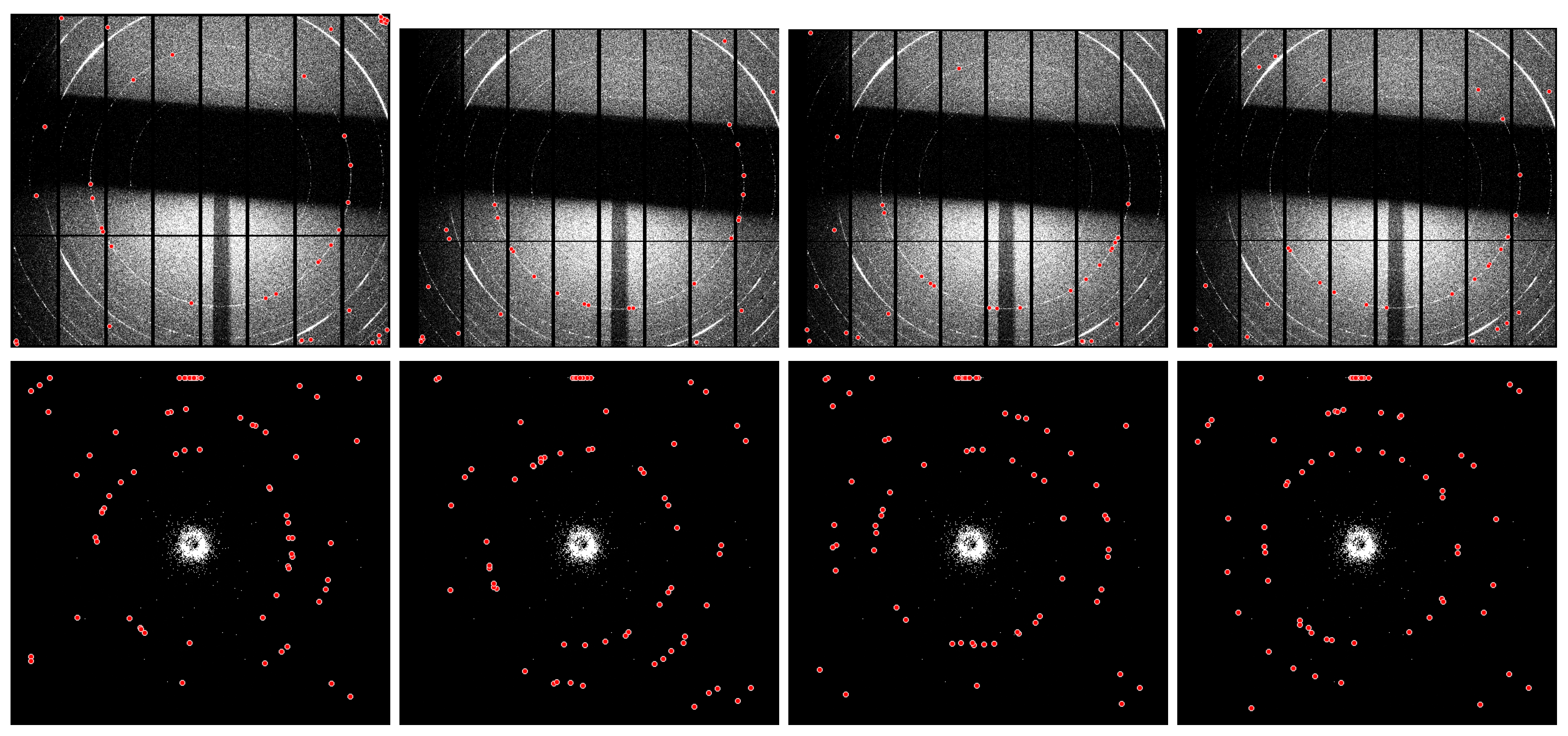
Figure 2.
2D pattern obtained for the S04388 (top left), S04387 (top right) samples, both collected at the Synchrotron Radiation Facility, and 152762 (bottom left), resummed (bottom right) samples (together with centre closeup), collected at a table-top X-ray diffractometer. The red "×" symbol indicates the centre estimated by the (unsupervised) sniper2D algorithm when only the 2D intensity pattern is used as input, whereas the blue "+" symbol shows the centre obtained by applying the same algorithm to the combined 2D intensity–phase pattern.
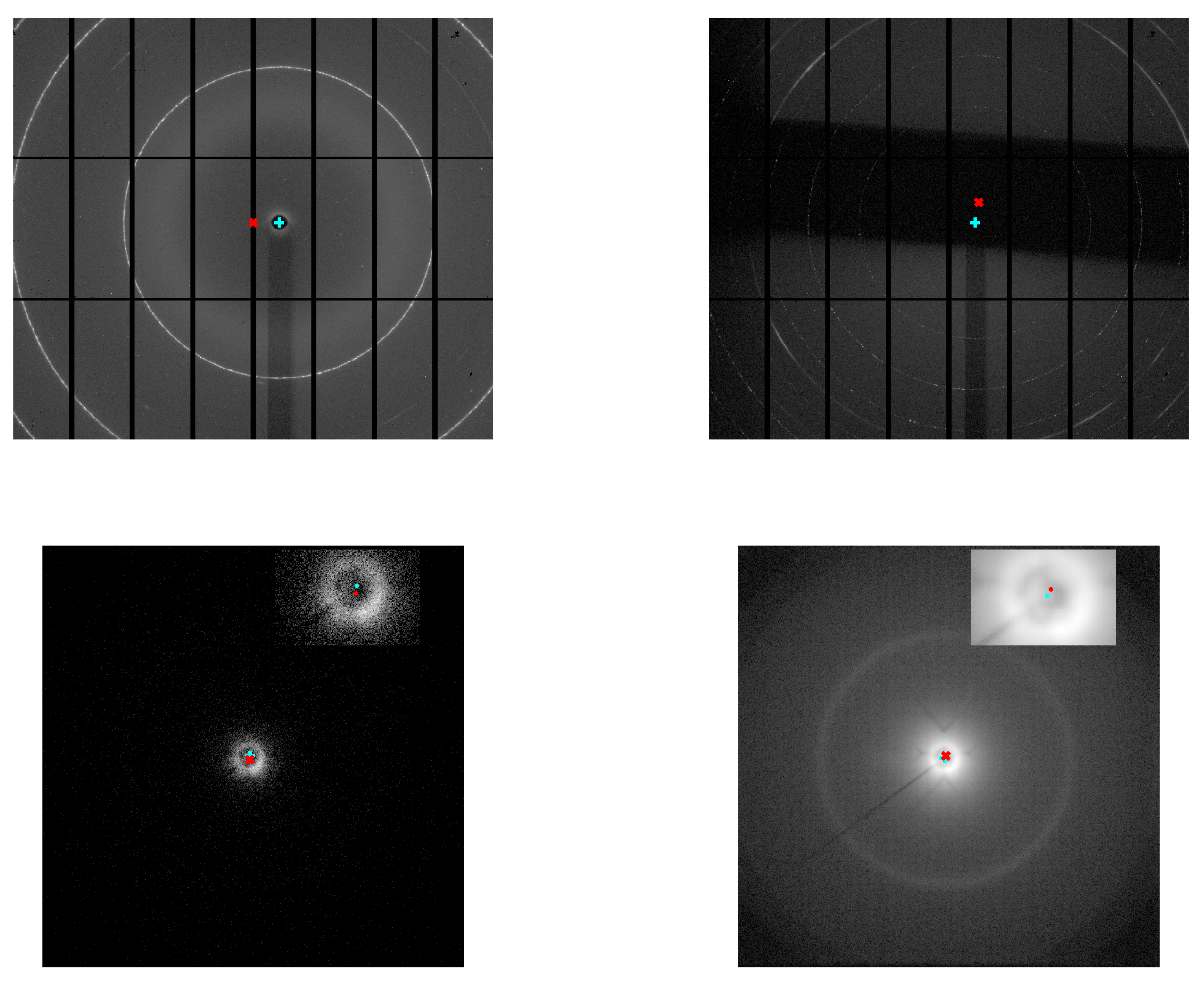
Figure 3.
1D profiles and 2D conformal maps for the S04387 sample background: (top left) this work, (top right) ImageJ with a 25-pixel ball radius, (bottom left) ImageJ with a 50-pixel ball radius, and (bottom right) ImageJ with a 100-pixel ball radius.
Figure 3.
1D profiles and 2D conformal maps for the S04387 sample background: (top left) this work, (top right) ImageJ with a 25-pixel ball radius, (bottom left) ImageJ with a 50-pixel ball radius, and (bottom right) ImageJ with a 100-pixel ball radius.
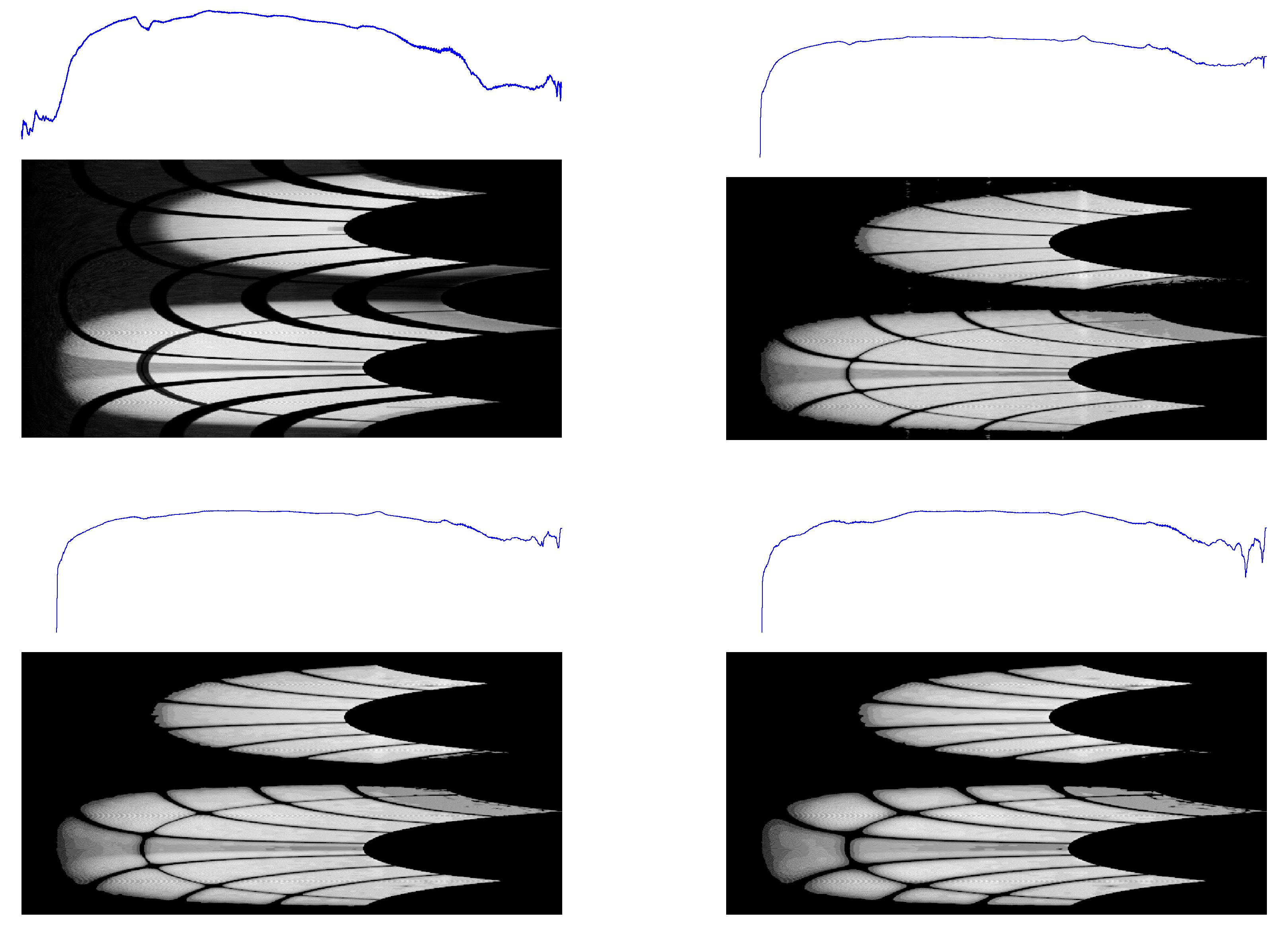
Figure 4.
1D profiles and 2D conformal maps for the sam4 sample background: (top left) this work, (top right) ImageJ with a 25-pixel ball radius, (bottom left) ImageJ with a 50-pixel ball radius, and (bottom right) ImageJ with a 100-pixel ball radius.
Figure 4.
1D profiles and 2D conformal maps for the sam4 sample background: (top left) this work, (top right) ImageJ with a 25-pixel ball radius, (bottom left) ImageJ with a 50-pixel ball radius, and (bottom right) ImageJ with a 100-pixel ball radius.
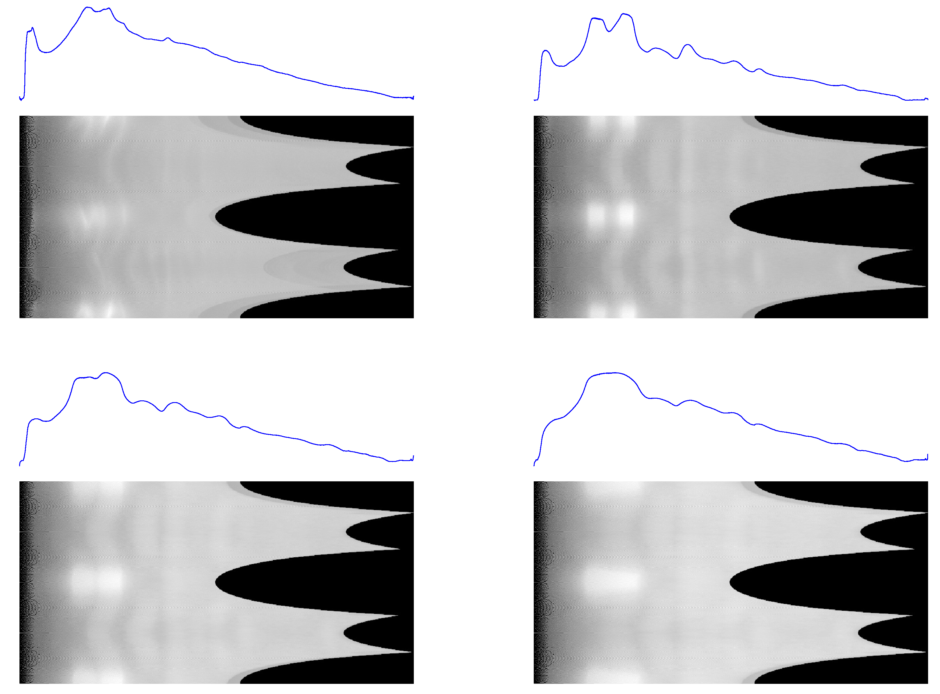
Figure 5.
Semilogarithmic profiles obtained for the sam4 (left) and S04387 (right) sample backgrounds.
Figure 5.
Semilogarithmic profiles obtained for the sam4 (left) and S04387 (right) sample backgrounds.
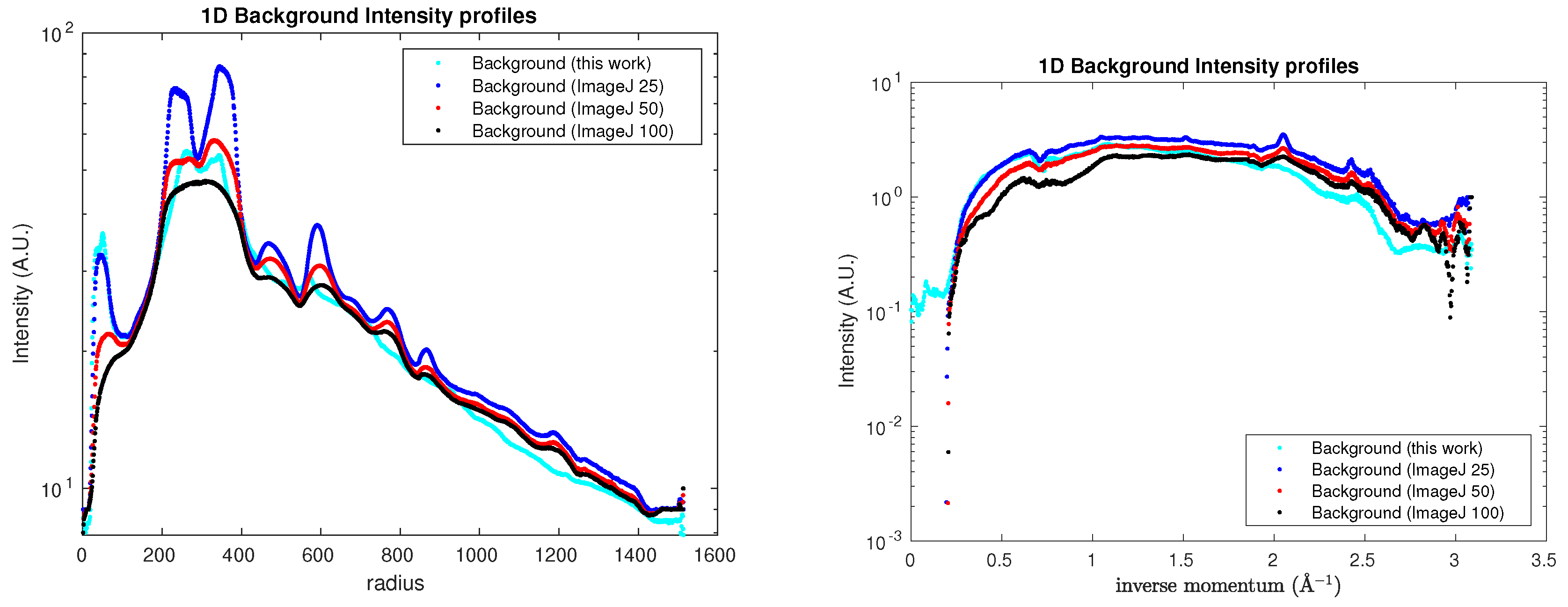
Figure 6.
1D profiles and 2D conformal maps for the rat tail sample: unprocessed (top left), denoised (top right), background (bottom left), denoised and background subtracted (bottom right).
Figure 6.
1D profiles and 2D conformal maps for the rat tail sample: unprocessed (top left), denoised (top right), background (bottom left), denoised and background subtracted (bottom right).
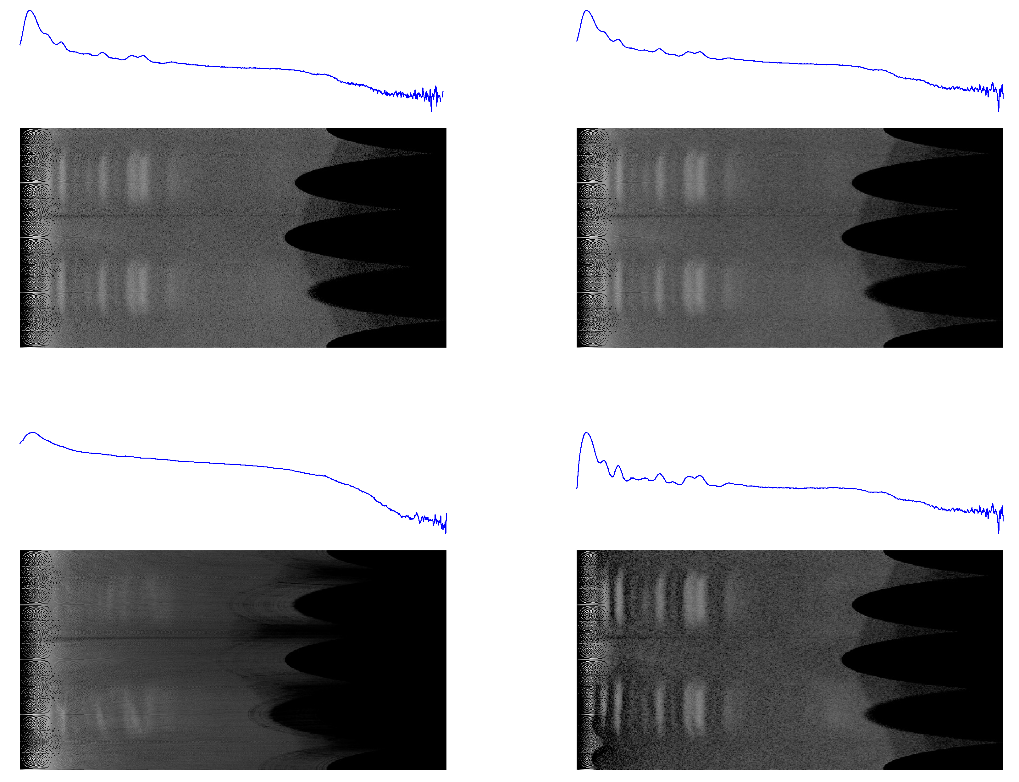
Figure 7.
1D semilogarithmic profiles and 2D original maps obtained for the rat tail (left) and sam4 (right) samples.
Figure 7.
1D semilogarithmic profiles and 2D original maps obtained for the rat tail (left) and sam4 (right) samples.
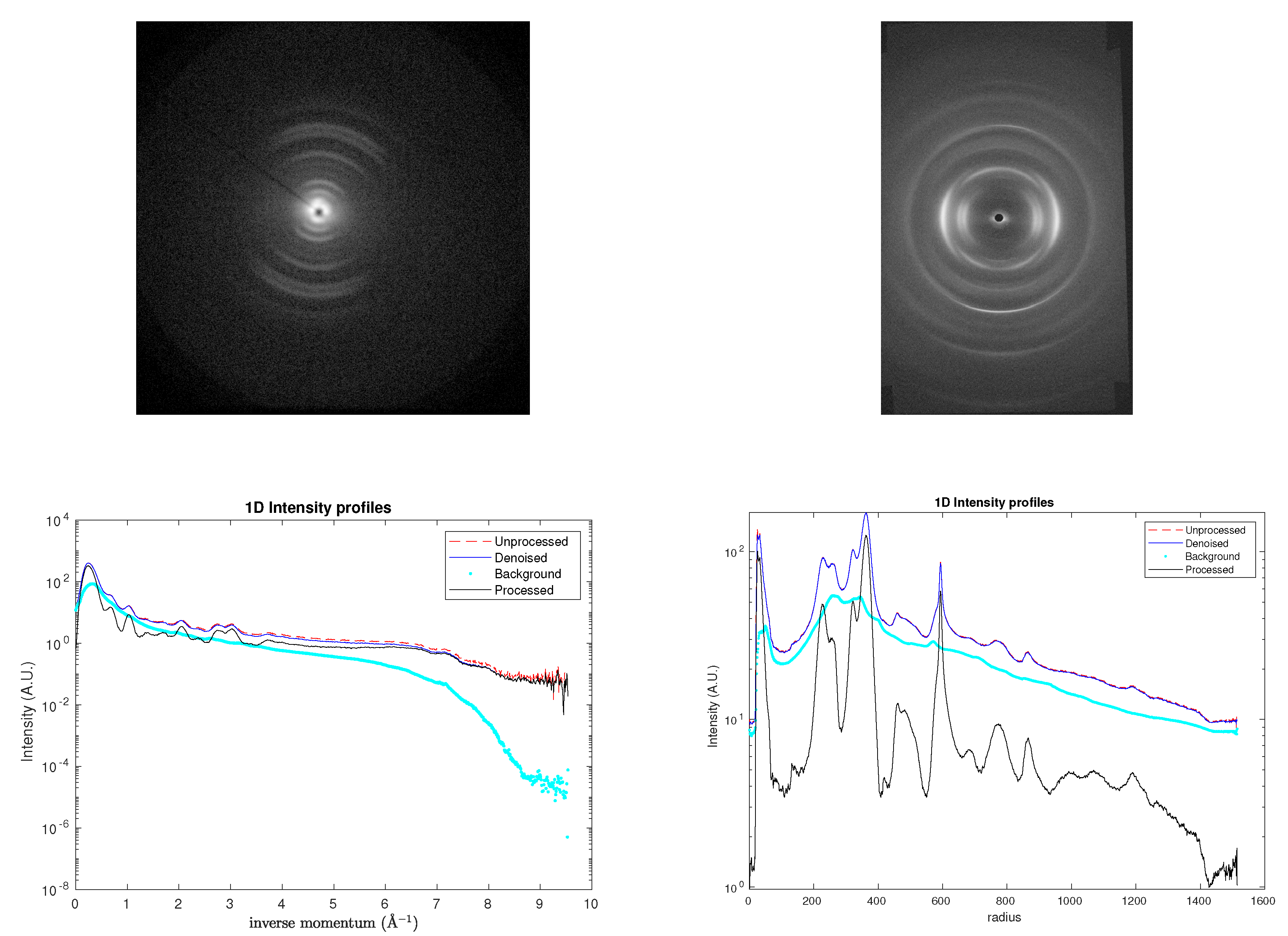
Figure 8.
Semilogarithmic intensity profiles for the rat tail (top left), sam4 (top right), S04387 (bottom left), and S04388 (bottom right) samples. For reference, analogous profiles obtained with Dioptas are also included.
Figure 8.
Semilogarithmic intensity profiles for the rat tail (top left), sam4 (top right), S04387 (bottom left), and S04388 (bottom right) samples. For reference, analogous profiles obtained with Dioptas are also included.
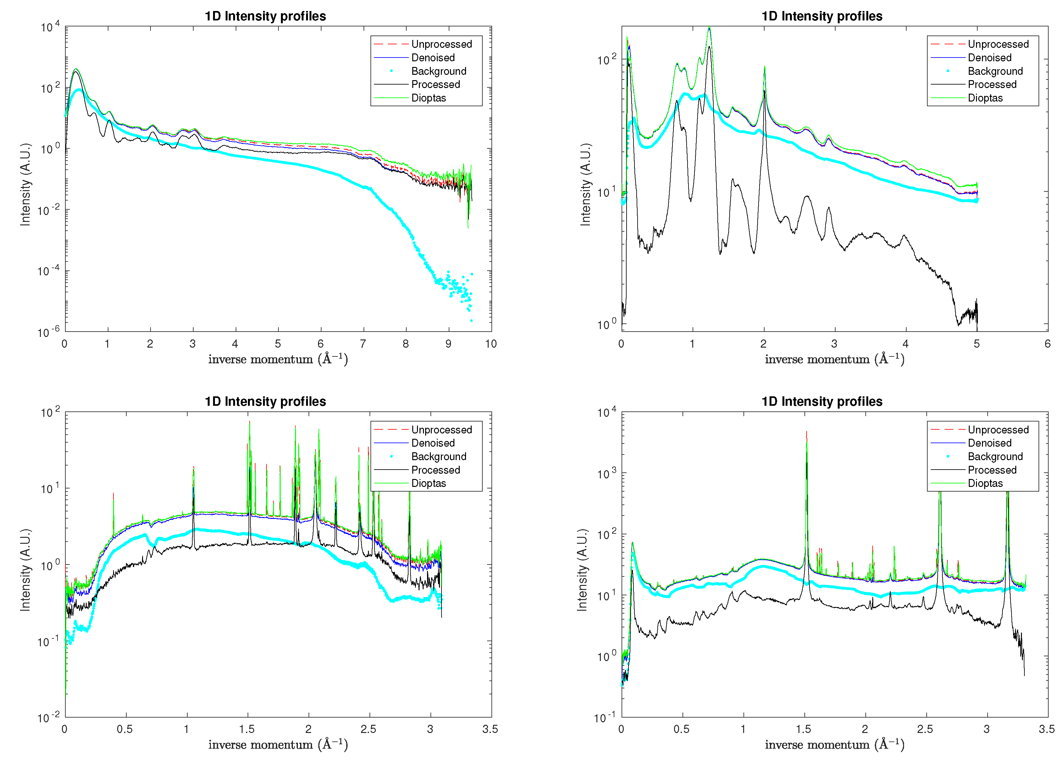
Figure 9.
1D semilogarithmic profiles (right) and 2D original maps (left) obtained for the rat tail sample at different exposure times: 2400 s (top), 171568 s (centre), and 327350 s (bottom). For reference, analogous profiles obtained with Dioptas are also included.
Figure 9.
1D semilogarithmic profiles (right) and 2D original maps (left) obtained for the rat tail sample at different exposure times: 2400 s (top), 171568 s (centre), and 327350 s (bottom). For reference, analogous profiles obtained with Dioptas are also included.
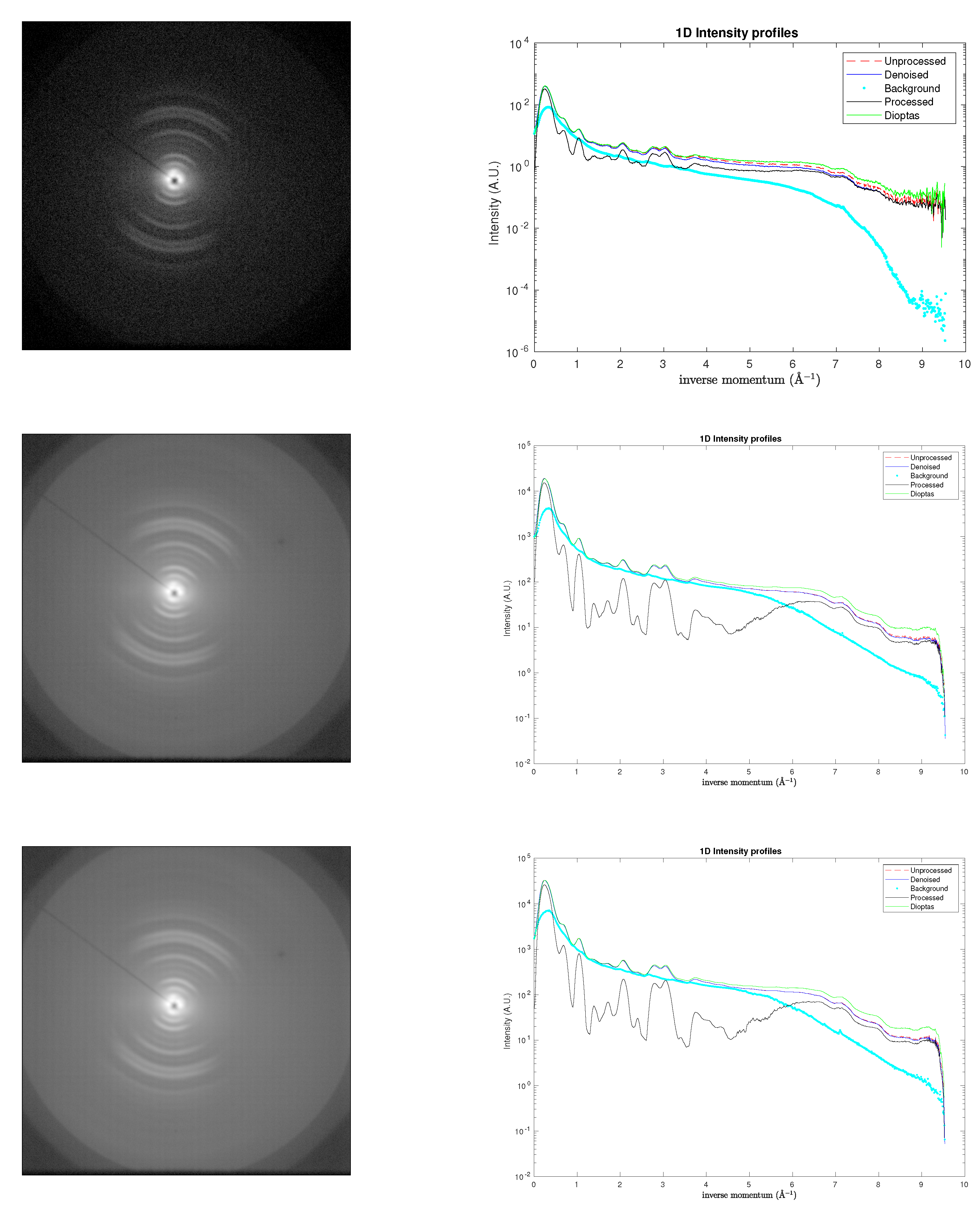
Figure 10.
1D profiles and 2D conformal maps for the sam4 sample: unprocessed (top left), denoised (top right), background (bottom left), denoised and background subtracted (bottom right).
Figure 10.
1D profiles and 2D conformal maps for the sam4 sample: unprocessed (top left), denoised (top right), background (bottom left), denoised and background subtracted (bottom right).
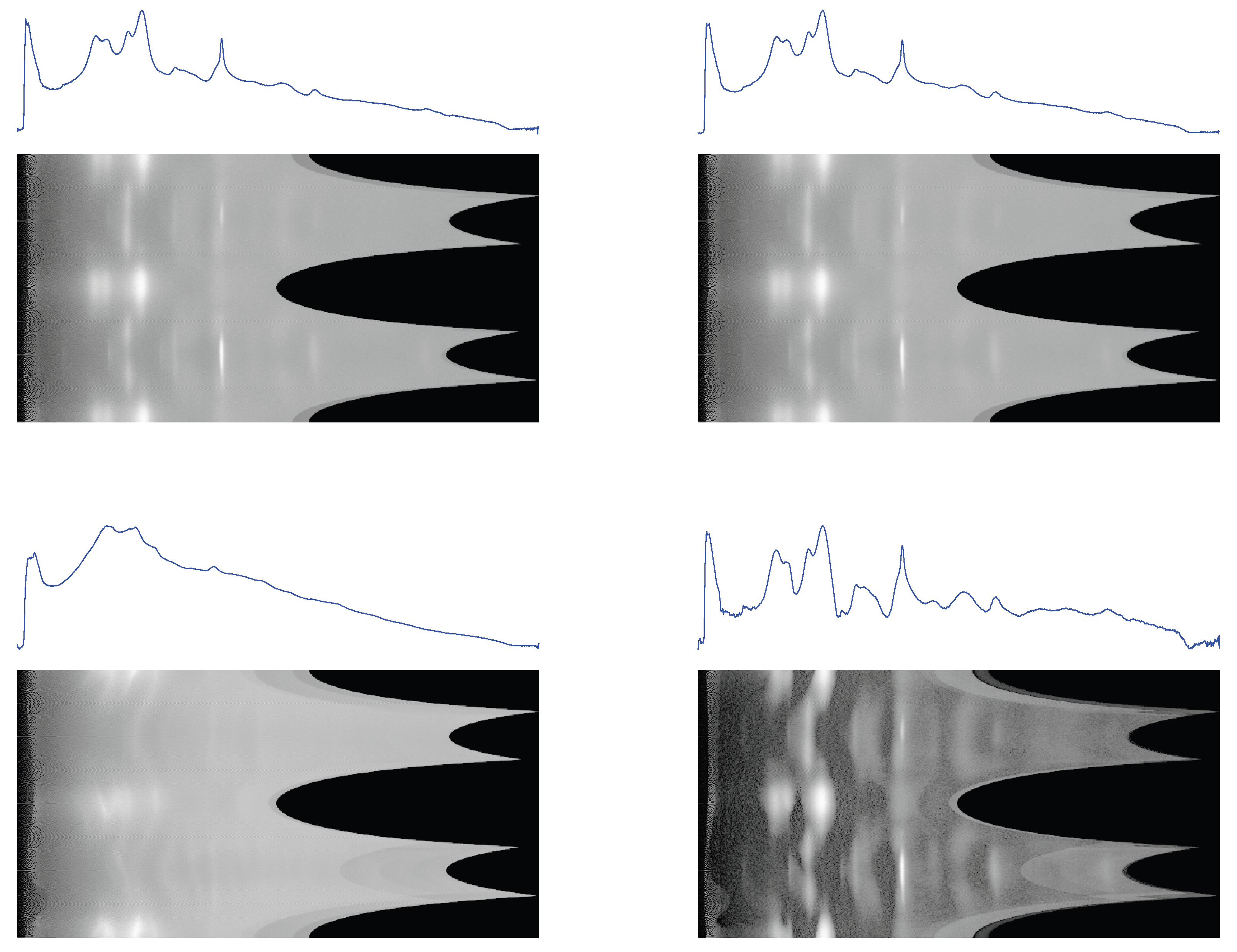
Figure 11.
1D profiles and 2D conformal maps for the S04387 sample: unprocessed (top left), denoised (top right), background (bottom left), denoised and background subtracted (bottom right).
Figure 11.
1D profiles and 2D conformal maps for the S04387 sample: unprocessed (top left), denoised (top right), background (bottom left), denoised and background subtracted (bottom right).
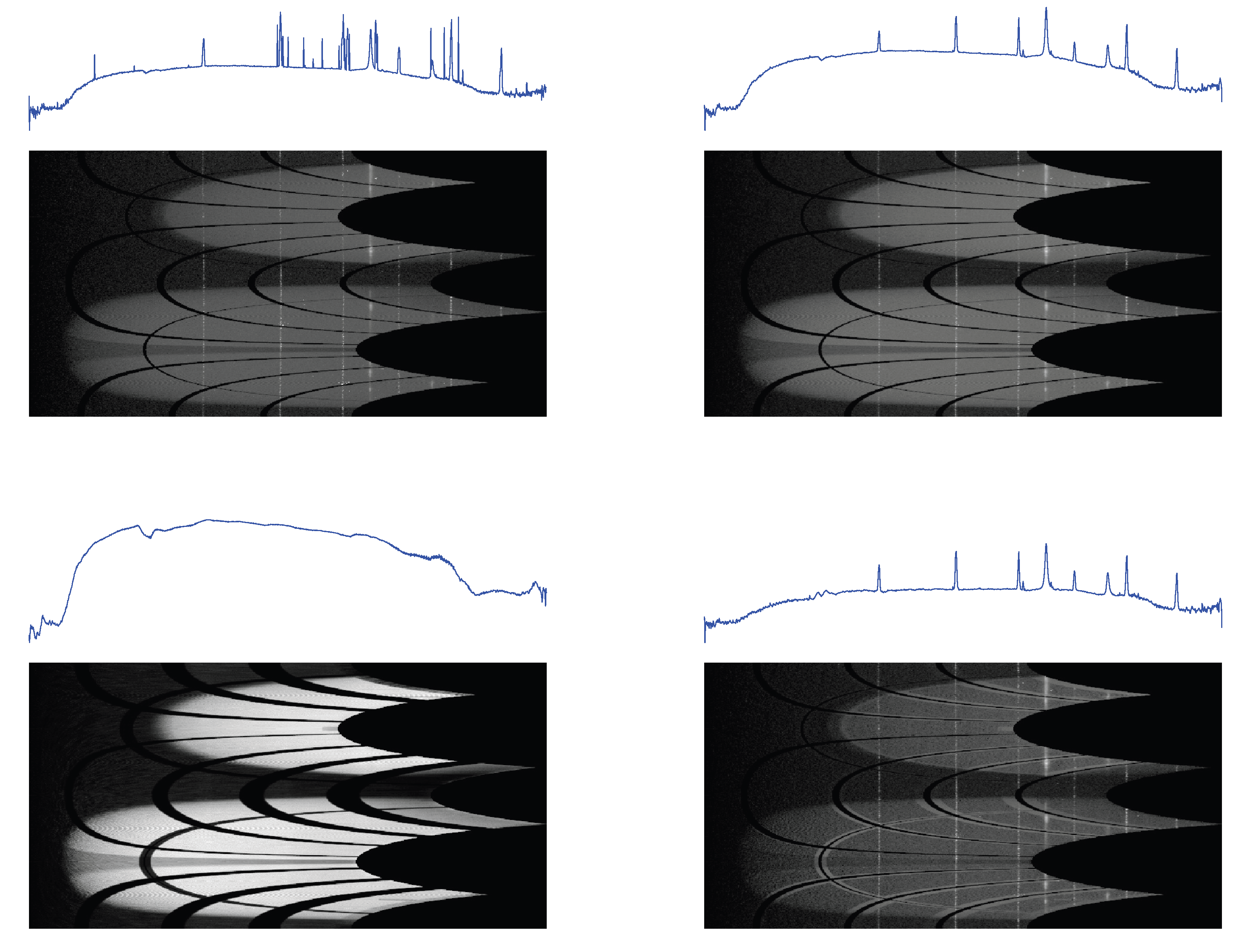
Figure 12.
1D profiles and 2D conformal maps for the S04388 sample: unprocessed (top left), denoised (top right), background (bottom left), denoised and background subtracted (bottom right).
Figure 12.
1D profiles and 2D conformal maps for the S04388 sample: unprocessed (top left), denoised (top right), background (bottom left), denoised and background subtracted (bottom right).
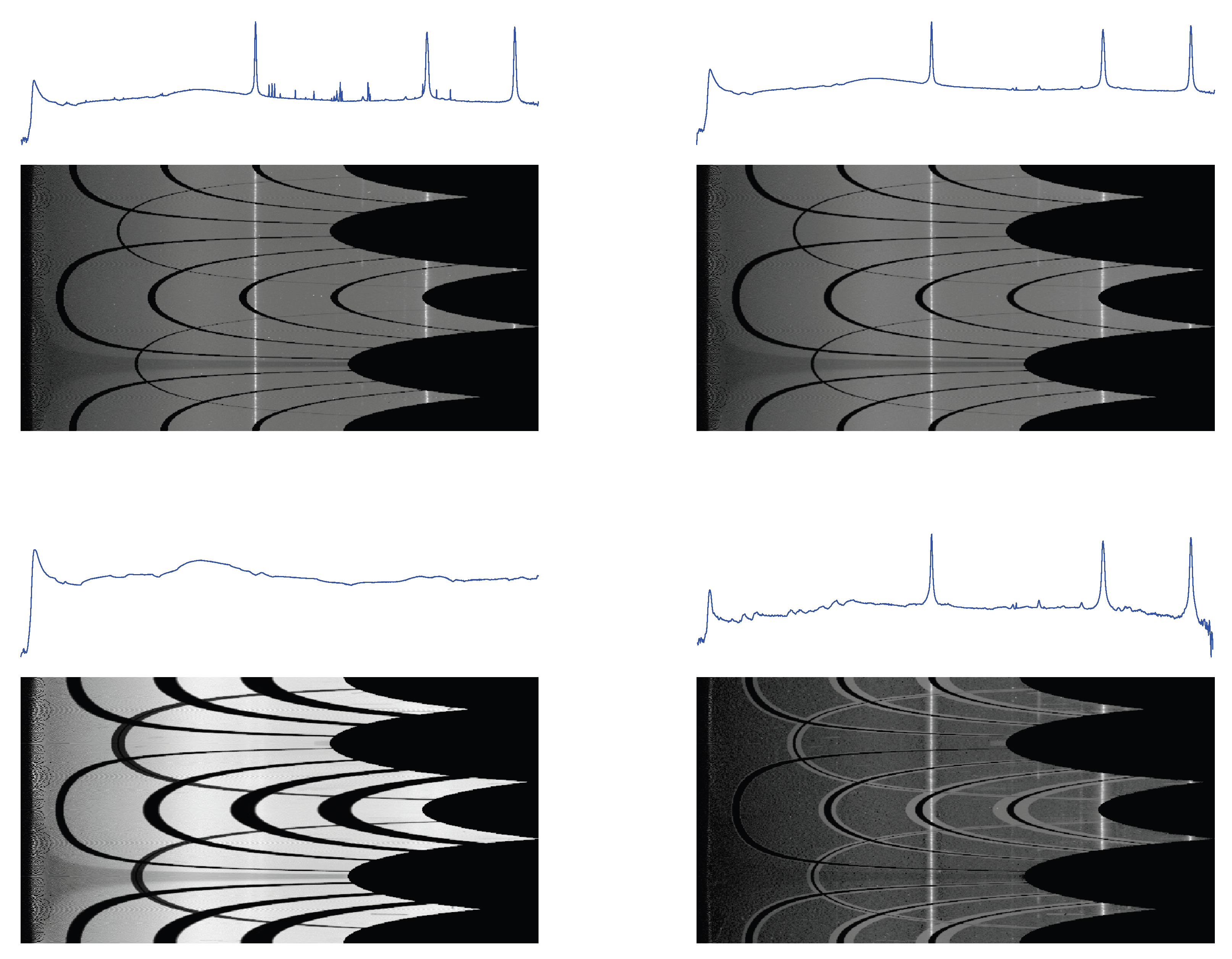

Table 1.
Metrics for diffraction ring analysis: intensity entropy , correlation with (), joint entropy and ring centers determined by this work versus Dioptas.
Table 1.
Metrics for diffraction ring analysis: intensity entropy , correlation with (), joint entropy and ring centers determined by this work versus Dioptas.
| Sample | exp. time (s) | I– corr. | Centre (this work) | Centre (Dioptas) | ||
|---|---|---|---|---|---|---|
| S04387 | - | 0.20 | 0.113 | 0.14 | (932,717) | (931,717) |
| S04388 | - | 0.33 | 0.017 | 0.24 | (931,717) | (935,720) |
| rat-tail | 2400 | 0.19 | -0.006 | 0.14 | (475,494) | (486,497) |
| rat-tail | 171568 | 0.35 | -0.005 | 0.28 | (474,493) | (486,497) |
| rat-tail | 327350 | 0.35 | 0.004 | 0.29 | (476,493) | (486,497) |
| sam4 | 1800 | 0.35 | -0.010 | 0.30 | (753,1255) | (757,1254) |
| 152762 | 45 | 0.01 | 0.021 | 0.008 | (504,510) | (504,515) |
Table 2.
Metrics for the S04387 and sam4 sample 2D backgrounds: Pearson’s correlation (Corr), Structural Similarity Index (SSIM) and residuals (Res) are shown for a comparison between the results of the present work (Bckg) and those obtained using the ImageJ software (Bckg ImJx) with three different choices of rolling-ball radius (x=25/50/100 pixels).
| Sample | Corr(Bckg,Bckg ImJx) | SSIM(Bckg vs Bckg ImJx) | Res = | |
|---|---|---|---|---|
| x=25/50/100 | x=25/50/100 | x=25/50/100 | ||
| S04387 | 0.03 | 0.91/0.92/0.90 | 0.55/0.55/0.53 | 0.015/0.012/0.012 |
| sam4 | 0.59 | 0.90/0.96/0.96 | 0.90/0.91/0.91 | 0.25/0.11/0.10 |
Disclaimer/Publisher’s Note: The statements, opinions and data contained in all publications are solely those of the individual author(s) and contributor(s) and not of MDPI and/or the editor(s). MDPI and/or the editor(s) disclaim responsibility for any injury to people or property resulting from any ideas, methods, instructions or products referred to in the content. |
© 2025 by the author. Licensee MDPI, Basel, Switzerland. This article is an open access article distributed under the terms and conditions of the Creative Commons Attribution (CC BY) license (https://creativecommons.org/licenses/by/4.0/).
Copyright: This open access article is published under a Creative Commons CC BY 4.0 license, which permit the free download, distribution, and reuse, provided that the author and preprint are cited in any reuse.


