
Submitted:
14 December 2025
Posted:
16 December 2025
You are already at the latest version
Abstract
A harmonic analysis of Antarctic ice core proxy temperature, CO₂ and CH₄ data is presented spanning 350,000 years. To ensure consistent phase comparison, CO₂ data were converted from AICC2012 to EDC3 chronology using depth as the invariant coordinate. Using a greedy algorithm to select periodic components, the analysis initially obtained 59 periods for temperature but subsequently refined this to 55 periods after removing four components (22,150, 9,000, 8,000, and 4,540 years) that exhibited high correlations in the normalized covariance matrix. This refinement ensures stable, well-conditioned parameter estimates while maintaining excellent fits: R² = 0.952 for temperature and R² = 0.964 for CO₂ (truncated at 1515 CE), R² = 0.873 for CH₄. The algorithm independently recovers the canonical Milankovitch orbital periods (approximately 100,000, 41,000, and 23,000 years) without prior specification, validating both the methodology and the orbital pacing of ice ages (Milankovitch, 1941). Phase analysis reveals a systematic pattern of CO₂ lagging temperature at orbital timescales, with mean lag approximately 1,700 years, consistent with the hypothesis that temperature drives CO₂ through ocean degassing rather than the reverse. Examination of the Last Interglacial (Eemian) reveals a striking asymmetry: CO₂ remained elevated at 275–280 ppm for approximately 13,000 years while temperature declined by 7°C. An R² analysis clearly reveals the Mid-Pleistocene Transition and justifies limiting the input to the fit. The modern CO₂ spike, which departs dramatically from the 350,000-year orbital envelope, is clearly anomalous relative to the harmonic structure of the paleoclimate record.
Keywords:
ice-core
; Antarctic
; CO₂
; CH₄
; MPT
1. Introduction
The relationship between atmospheric CO₂ and temperature over glacial-interglacial cycles has been extensively studied using ice core records. A central question concerns causality: does CO₂ drive temperature through radiative forcing, or does temperature drive CO₂ through effects on ocean solubility, biological productivity, and terrestrial carbon storage?
Previous studies have established that CO₂ variations lag temperature changes during glacial terminations by several hundred to a few thousand years (Humlum et al., 2013; Grabyan, 2025). However, the precise phase relationship varies across different studies depending on methodology. Here we apply harmonic analysis with a novel period-selection algorithm to Antarctic ice core data spanning the last 350,000 years.
Related work includes Higginbotham (2025a), which analyzes sea level using planetary-orbit–related periodicities, and Higginbotham (2025b), which examines water vapor and volcanic influences, including the 13,000-year interval in which CO₂ remained high while temperature fell by about 7 °C
2. Data and Methods
2.1. Data Sources and Chronology
We analyze Antarctic ice core data from the EPICA Dome C (EDC) record. To ensure internally consistent phase comparisons between temperature, CO₂, and CH₄, all datasets were placed on the EDC3 chronology (Parrenin et al., 2007).
Temperature: EPICA Dome C deuterium-derived temperature proxy (Jouzel et al., 2007), EDC3 chronology, 4,752 data points from 350,245 years BP to 1911 CE.
CO₂: Antarctic composite record (Bereiter et al., 2015), originally on AICC2012 chronology (Bazin et al., 2013; Veres et al., 2013). Gas ages were converted to EDC3 chronology as described in Section 2.2. Data truncated at 1515 CE due to limitations of the gas age conversion (see Section 2.2). The fit involved 1,130 data points from 350,000 BCE to 1515 CE.
CH₄: EPICA Dome C methane record (Loulergue et al., 2008), EDC3 gas age chronology, matching the temperature chronology. The fit involved 1,418 data points from 350,000 BCE to 1824 CE.
In the tables and figures that follow, negative dates correspond to BCE while positive dates correspond to CE.
2.2. Chronology Conversion for CO₂ Data
The CO₂ composite record (Bereiter et al., 2015) was published on the AICC2012 chronology, while the temperature and CH₄ records are on the EDC3 chronology. To enable direct phase comparison between records, the CO₂ gas ages were converted from AICC2012 to EDC3.
Both chronologies share a common depth scale for the EPICA Dome C core. Depth is the invariant physical coordinate measured during core extraction; the chronologies represent different mathematical models that assign ages to those depths based on different constraints and methodologies. The conversion was performed by:
- Constructing a mapping table between AICC2012 and EDC3 gas ages using depth as the parametric coordinate
- For each CO₂ data point, interpolating its AICC2012 gas age to the corresponding EDC3 gas age
The chronology differences are non-uniform with depth. AICC2012 is on average approximately 0.7 ka older than EDC3, with a standard deviation of 1.0 ka. The maximum deviation (approximately 5–6 ka) occurs around Marine Isotope Stage 12 (400–430 ka) and near the base of the core (>700 ka). For the interval analyzed here (0–350 ka), differences are typically within ±3 ka.
A three-way conversion table encompassing EDC3, AICC2012, and the more recent AICC2023 chronology (Bouchet et al., 2023) is provided in Supplementary Table S1. The AICC2023 chronology incorporates ⁸¹Kr absolute dating constraints but was not used in this analysis to maintain consistency with the EDC3 framework of the temperature record.
We note that the CO₂ composite includes data from multiple Antarctic cores. The portions derived from Law Dome, WAIS, and Siple Dome cores are not on AICC2012; applying the EDC-specific conversion to these non-EDC data points produces chronological disorder in the most recent ~2,000 years of the converted record. This has no effect on the harmonic analysis, as least-squares fitting evaluates each data point independently regardless of temporal ordering. The CO₂ record is truncated at 1515 CE due to the lack of gas age data in the conversion table for the most recent portion; this truncation also excludes most of the affected multi-core interval and all anthropogenic influence.
Converting chronology can produce additional error in the data. Here the decision was made to convert the CO₂ data from AICC2012 to EDC3 because only one set of data required this conversion. Going from EDC3 to AICC2012 would require converting two sets of data. Going to AICC2023 would require converting three sets of data with possible ensuing errors. Still, if AICC2023 is more accurate then that conversion might have been the optimal path to take.
2.3. Natural Weighting from Sampling Density
Ice core data exhibits non-uniform temporal sampling density. Annual layers are thicker and more distinct in recent ice (though there are complications with firn analysis - firn is the crucial, granular stage of old, compacted snow that hasn’t yet turned into solid glacial ice) while deeper ice is compressed and harder to resolve temporally. For the EDC temperature record, sampling density is approximately one point per decade in the recent portion, decreasing to one point per several centuries in the oldest sections.
In an unweighted least-squares fit, each data point contributes equally to the residual sum of squares. With denser sampling in recent times, the optimization algorithm effectively weights the recent data more heavily—the last glacial cycle receives more statistical leverage than earlier cycles simply because it is sampled more finely.
This natural weighting is not a bias to be corrected but rather a consequence of where the data actually contains resolvable information. The denser sampling in recent ice reflects:
- Better preservation of high-frequency signals in less-compacted ice
- Reduced diffusion of trapped gases in shallower firn
- More resolvable annual layering for age control
The algorithm properly attends to data intervals with higher information content. Features such as the Younger Dryas cold event, the Holocene thermal optimum, and the Little Ice Age can be resolved in the recent record precisely because the sampling density supports detection of variations at millennial and sub-millennial timescales. Equivalent rapid events in the sparse older portions of the record would be invisible regardless of fitting methodology.
It seems obvious that when more data is available in a given time interval, that time interval has more statistical weight.
2.4. Harmonic Fitting Methodology
Each dataset is fit to a harmonic model of the form:
X(t) = C + Σᵢ Aᵢ sin(2π(t − t₀)/Pᵢ + φᵢ)
where C is a constant offset, t₀ is the time origin (−175,000 years for all fits to allow direct comparison of phase), and each periodic component has amplitude Aᵢ, period Pᵢ, and phase φᵢ. For computational stability, the model is implemented using sine and cosine basis functions:
X(t) = C + Σᵢ [aᵢ sin(2π(t − t₀)/Pᵢ) + bᵢ cos(2π(t − t₀)/Pᵢ)]
where amplitude A = √(a² + b²) and phase φ = atan2(a, b). This parameterization avoids nonlinear optimization over phase.
2.5. Greedy Period Selection Algorithm
Rather than using predetermined periods or standard Fourier analysis, we employ a “greedy” algorithm: beginning with a constant term, iteratively add the period that most reduces residual variance, searching continuously over period space. The algorithm includes safeguards against ill-conditioning: minimum period separation, rejection of candidates causing excessive amplitude changes in existing periods, and amplitude ceilings.
2.6. Covariance Matrix Analysis and Period Refinement
To verify that selected periods form a well-conditioned basis, we computed the normalized covariance matrix for fitted parameters. Off-diagonal elements near ±1 indicate near-collinearity, which inflates parameter uncertainties.
Using temperature as an example:
Initial analysis of the 59-period fit to temperature revealed problematic correlations:
- Periods 7,600 yr and 4,540 yr: r = −0.95
- Periods 8,900 yr and 9,000 yr: r = −0.70
- Periods 7,900 yr and 8,000 yr: r = −0.61
- Periods 23,000 yr and 22,150 yr: r = −0.51
We systematically removed the higher-index period from each problematic pair: 4,540, 9,000, 8,000, and 22,150 years. The final 55-period basis shows maximum off-diagonal correlations of |r| ≈ 0.15 for temperature and |r| ≈ 0.52 for CO₂—acceptable levels for stable parameter estimation.

Table 1.
Fit quality before and after covariance refinement.
| Configuration | R² (Temperature) | Max |r| |
| Original (59 periods) | 0.9539 | 0.95 |
| Refined (55 periods) | 0.9517 | 0.15 |
The minimal R² change (0.0022) confirms these components were largely redundant.
Where CO₂ and CH₄ were independently fit, the same procedure was followed to obtain a good R² with acceptable |r|.
2.7. Uncertainty Estimation from Covariance Matrix
The unnormalized covariance matrix provides variances for each fitted parameter. Standard errors (SE) on sine and cosine coefficients propagate to amplitude and phase uncertainties via:
SE(A) = √[(a/A)² var(a) + (b/A)² var(b)]
SE(φ) = (180/π) × √[(b/A²)² var(a) + (a/A²)² var(b)]
Phase lag uncertainties combine temperature and CO₂ phase uncertainties in quadrature:
SE(lag) = (P/360°) × √[SE(φ_T)² + SE(φ_CO₂)²]
2.8. CO₂ Fitting with Periods Found for Temperature
The CO₂ data was fit to the same 55 periods with constant, allowing only amplitudes and phases to vary. Data after 1515 CE was excluded. The truncated fit achieves R² = 0.964, with maximum off-diagonal correlation |r| = 0.52. See Supplementary Table S2 for fit parameters. The fit involved 1,130 data points.
2.9. CO₂ Fitting with Periods Found Independently
The fit to CO₂ with periods found independently, with data after 1515 CE excluded, used a constant and 46 periods achieving an R² = 0.966, with maximum off-diagonal correlation |r| < 0.55. The fit involved 1,130 data points.
2.10. CH₄ Fitting with Periods Found Independently
The fit to CH₄ with periods found independently used a constant and 55 periods achieving an R² = 0.873, with maximum off-diagonal correlation |r| = 0.40. The fit involved 1,418 data points.
2.11. Temperature Fitting over the Last Glacial Cycle (~137,000 Years)
An additional greedy algorithm fit was performed on temperature data spanning ~137,000 years (from −135,003 to 1911 CE), using finer 2-year period steps in the search. This extended span captures the full Eemian interglacial peak (~125,000 years ago) that shorter intervals miss, providing a complete glacial cycle from interglacial maximum through the Last Glacial Maximum to the Holocene. Because the time span still provides insufficient support to independently determine the longest orbital periods—the eccentricity period (113,600 yr) and obliquity period (40,200 yr)—these two periods were fixed at their values from the 350,000-year fit prior to the greedy search. The algorithm then found 31 additional periods, yielding a total of 33 periods plus constant (N = 34) with R² = 0.960 and residual σ = 0.75 °C. The fit used 3,211 data points, with approximately one period per 4,000 years of data span (one fitting parameter per 2,000 years), or equivalently one period per 94 input data points. Maximum off-diagonal correlation |r| < 0.50 after pruning correlated period pairs. See Supplementary Table S8 for fit parameters.
3. Results
3.1. Temperature Fit Quality
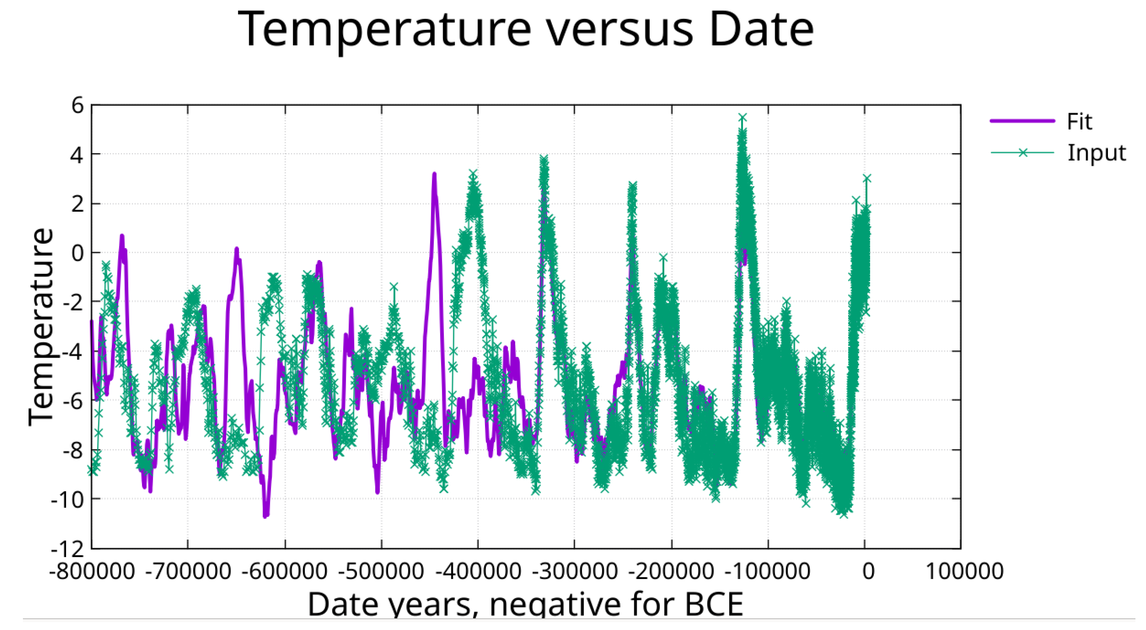
The 55-period fit achieves R² = 0.952, explaining over 95% of variance in the 350,000-year record. The fit tracks glacial-interglacial cycles, the Eemian peak, the last deglaciation, the Younger Dryas, and millennial-scale Holocene variations including the Little Ice Age. See Supplementary Table S3 for fit parameters. Additionally, fitting the entire temperature data set from ~800,000 BCE to 1911 CE with these same periods revealed the Mid-Pleistocene Transition, which is discussed in Section 3.6.
Figure 1.
Fit to temperature proxy from date -350,000 to date 1911.
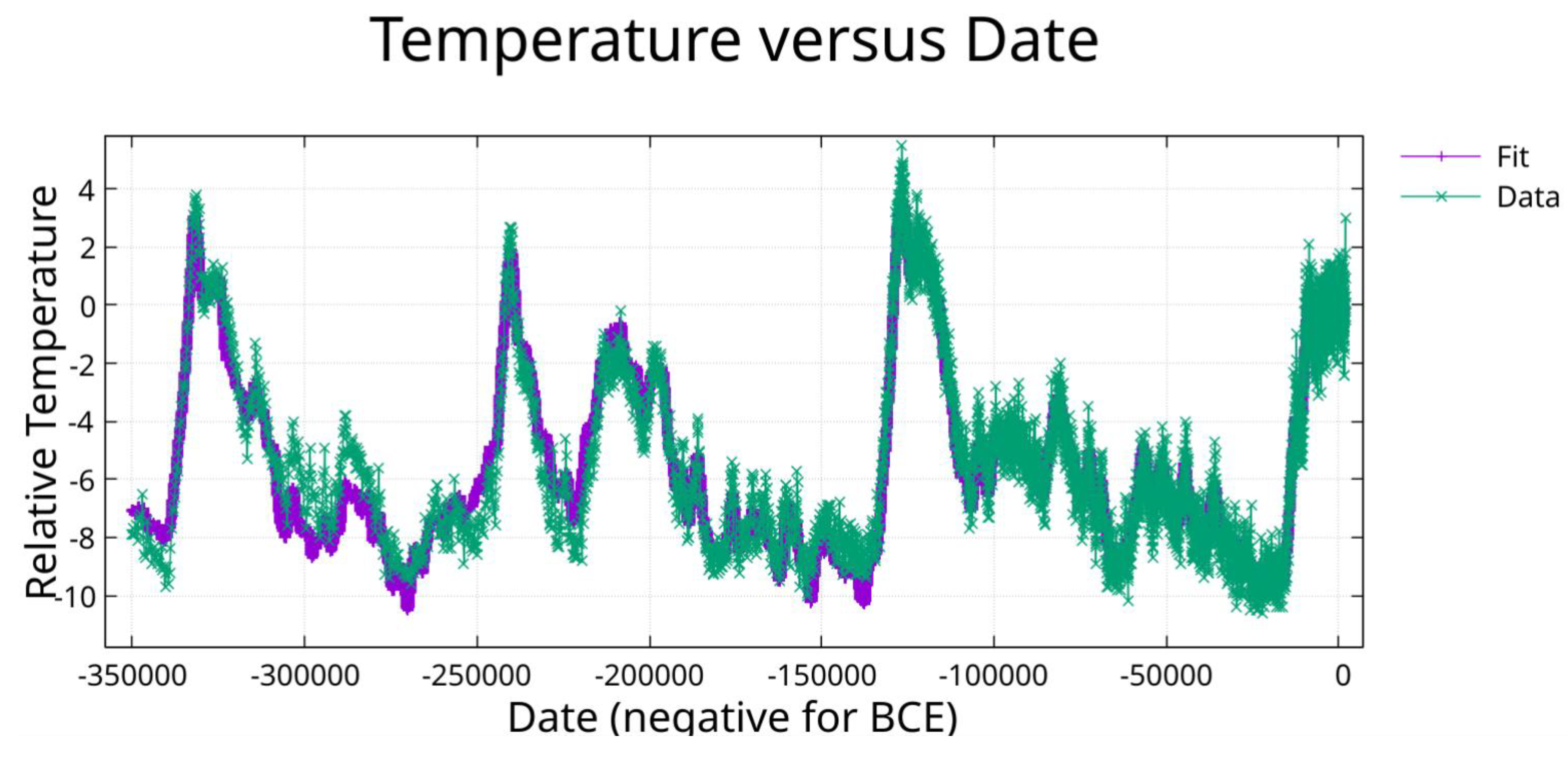
Figure 2.
Zoom on previous figure showing fit from -140,000 to 1911.
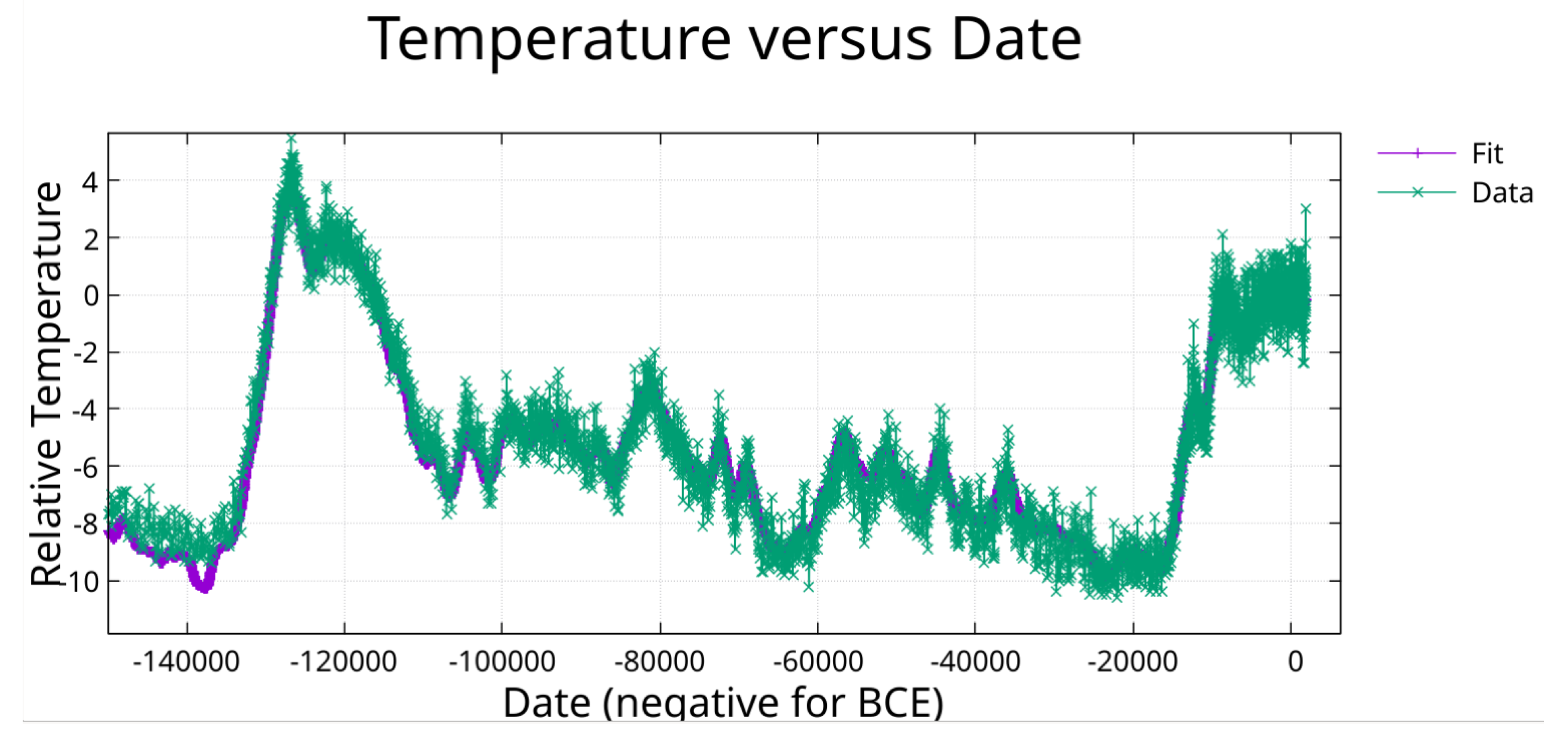
Figure 3.
Zoom on Figure 1 showing fit form -25000 to 1911.
Figure 3.
Zoom on Figure 1 showing fit form -25000 to 1911.
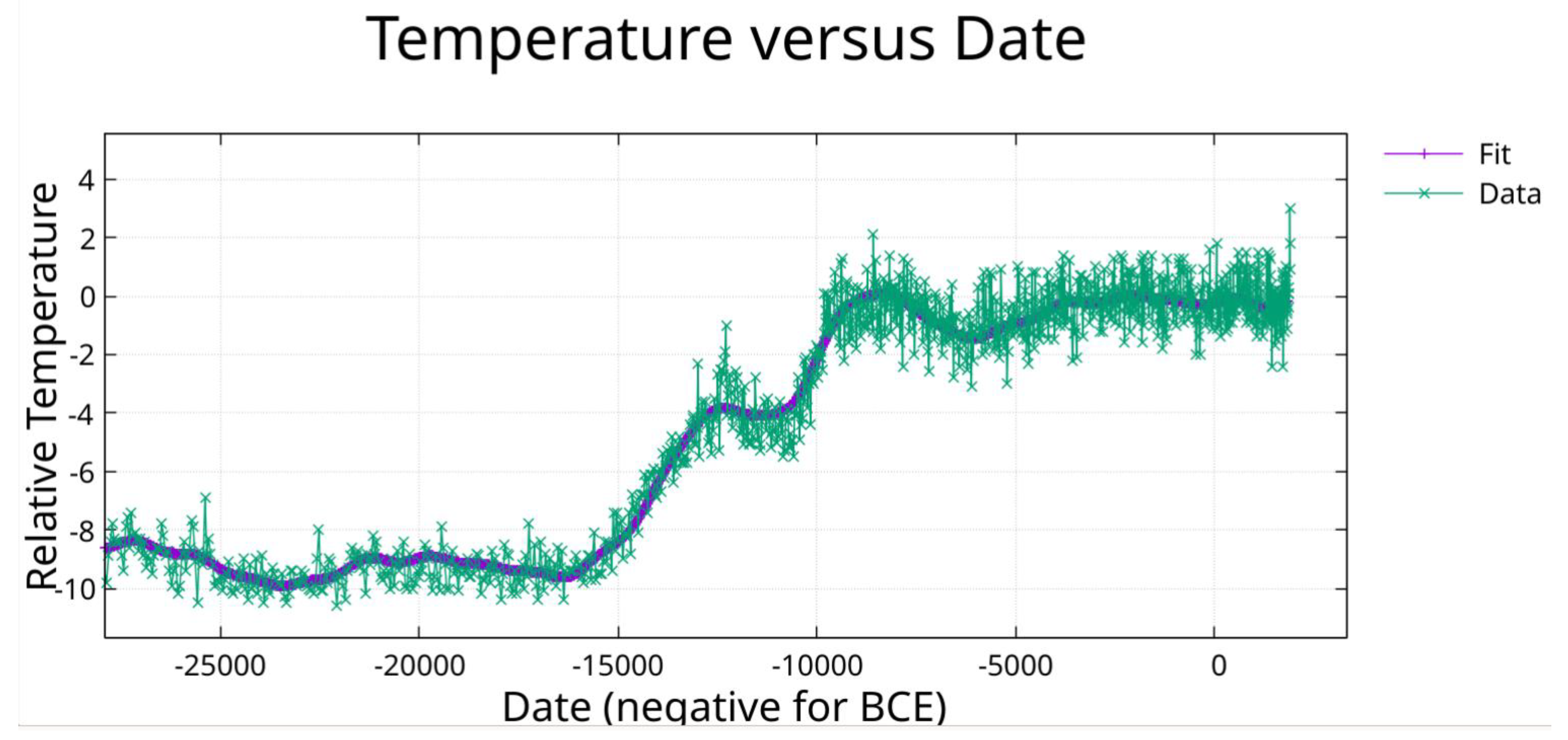
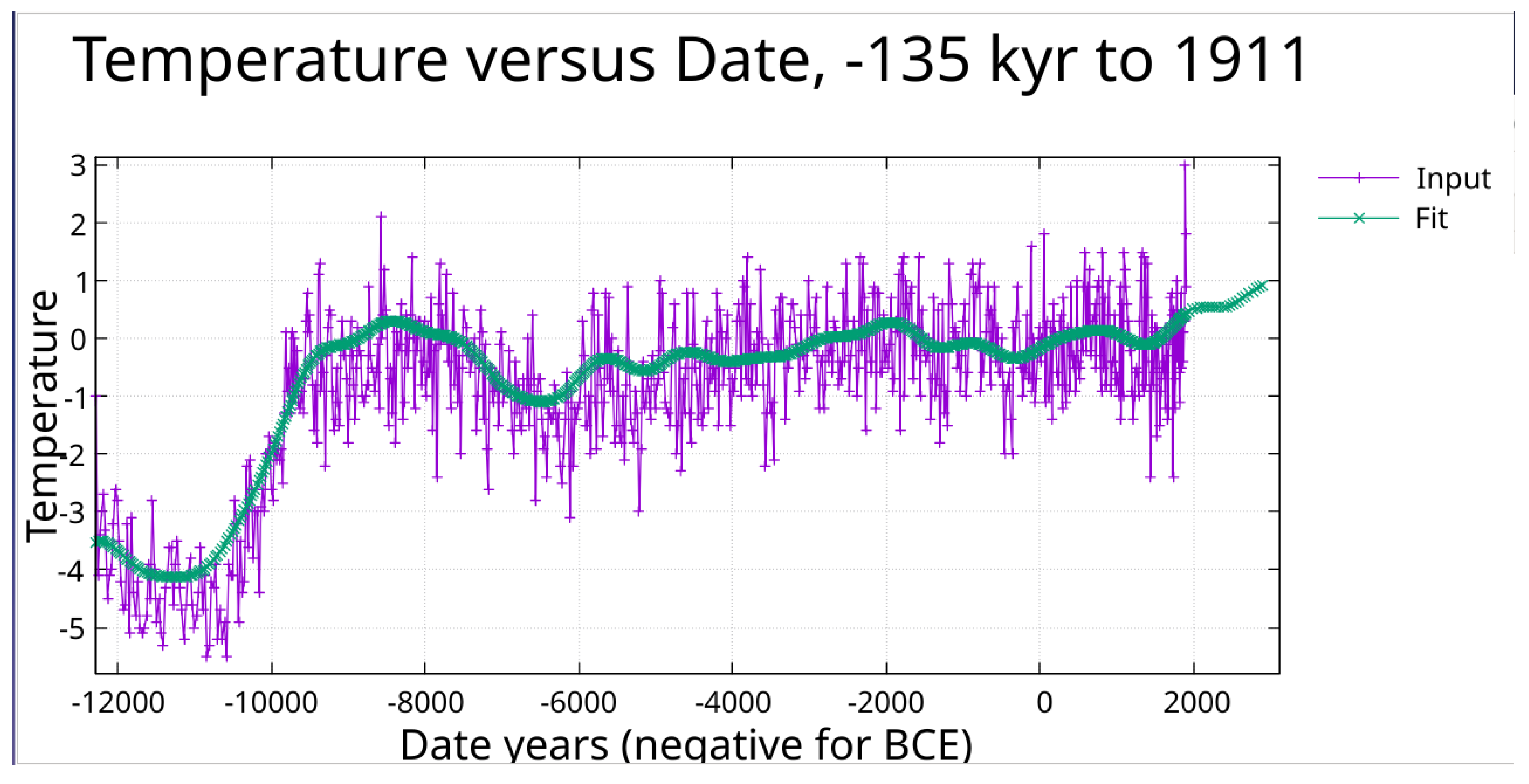
Figure 4.
Zoom on Figure 1 showing fit from -12000 to 1911.
Figure 4.
Zoom on Figure 1 showing fit from -12000 to 1911.
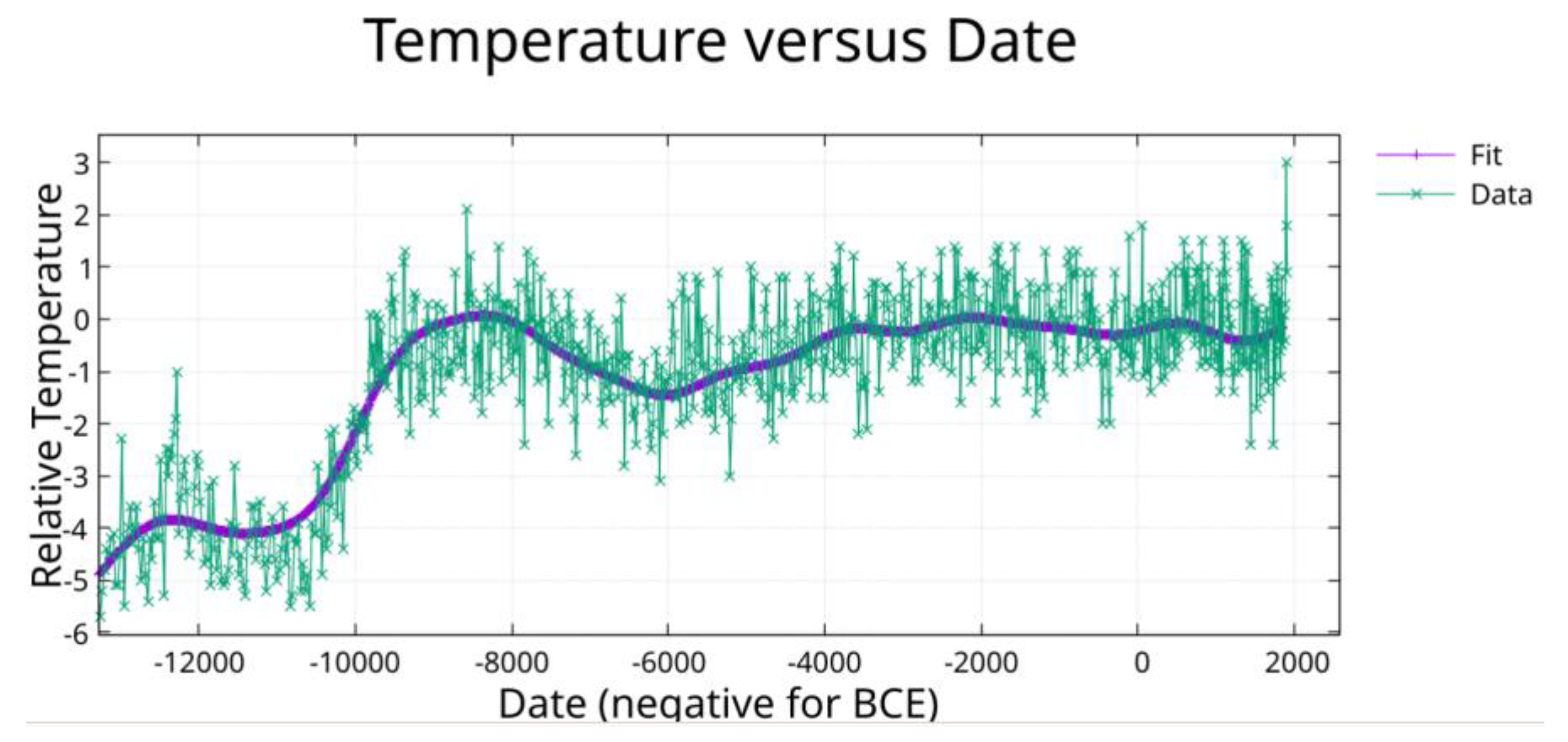
Figure 5.
Fit of CO₂ (periods from temperature fit) in ppm from date -350,000 to 1515.
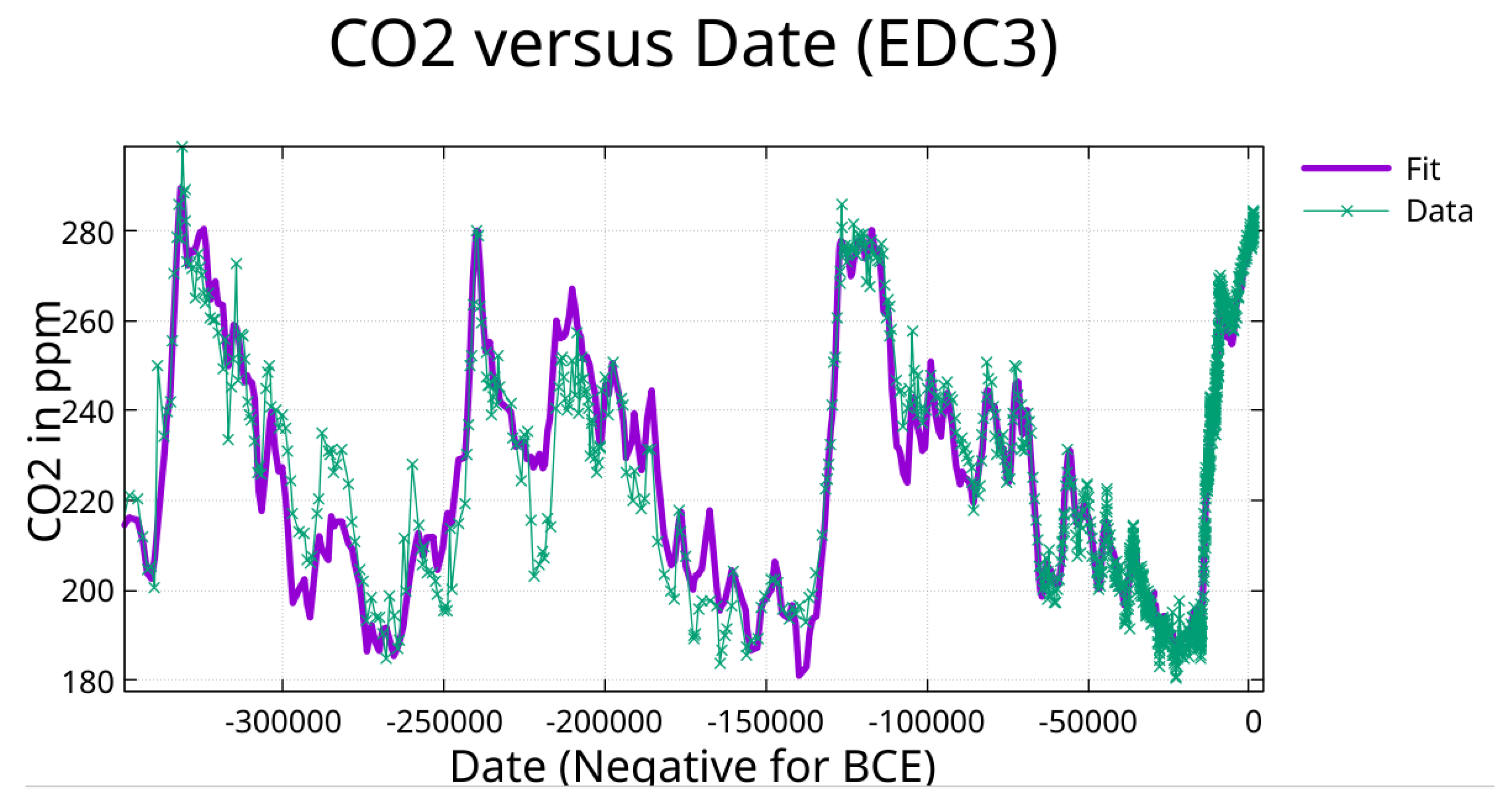
Figure 6.
Zoom on Figure 5 showing fit from prior interglacial warm period to date 1515.
Figure 6.
Zoom on Figure 5 showing fit from prior interglacial warm period to date 1515.
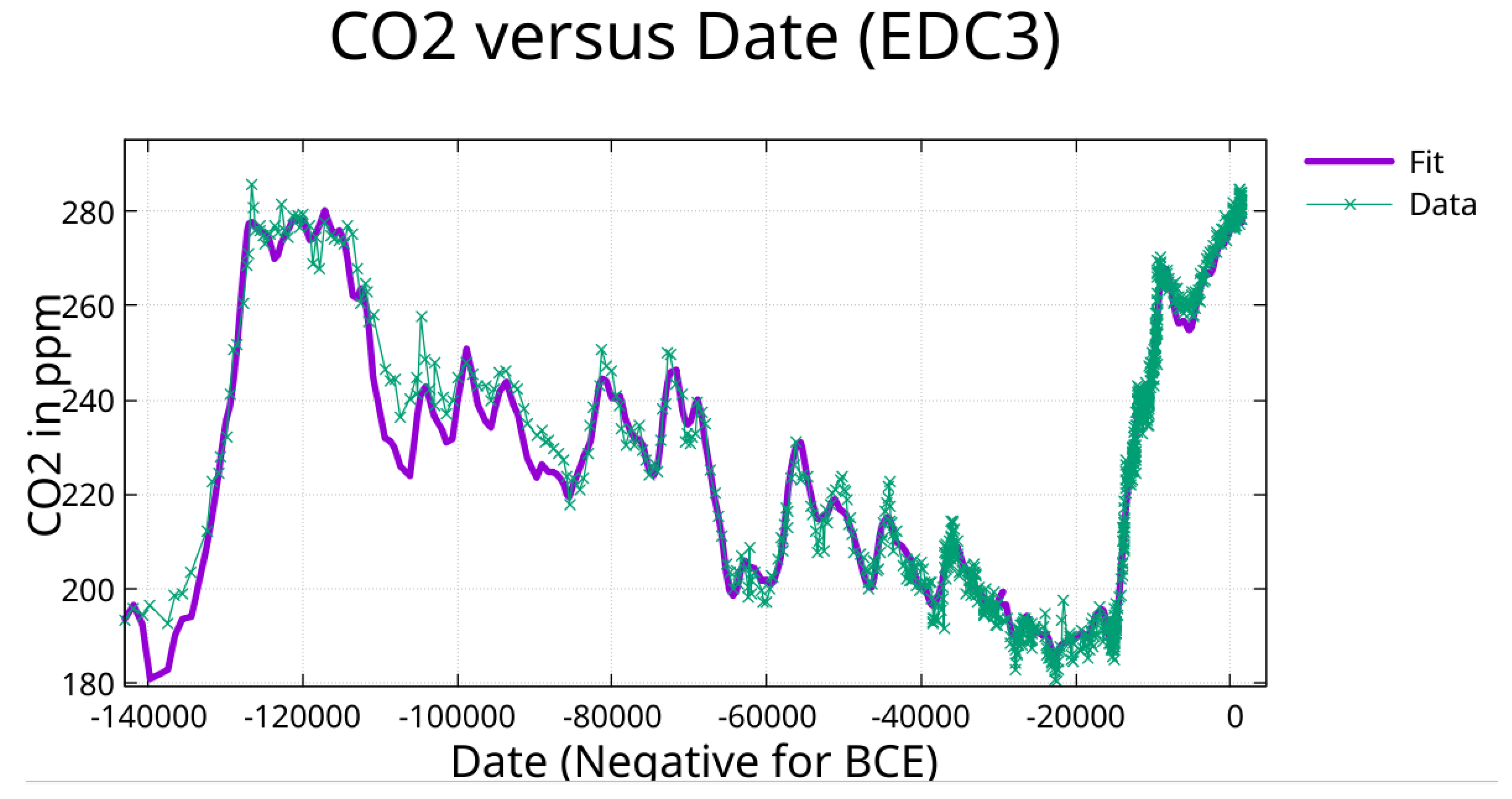
Figure 7.
Zoom on Figure 5 showing the fit from date -25,000 to date 1515.
Figure 7.
Zoom on Figure 5 showing the fit from date -25,000 to date 1515.
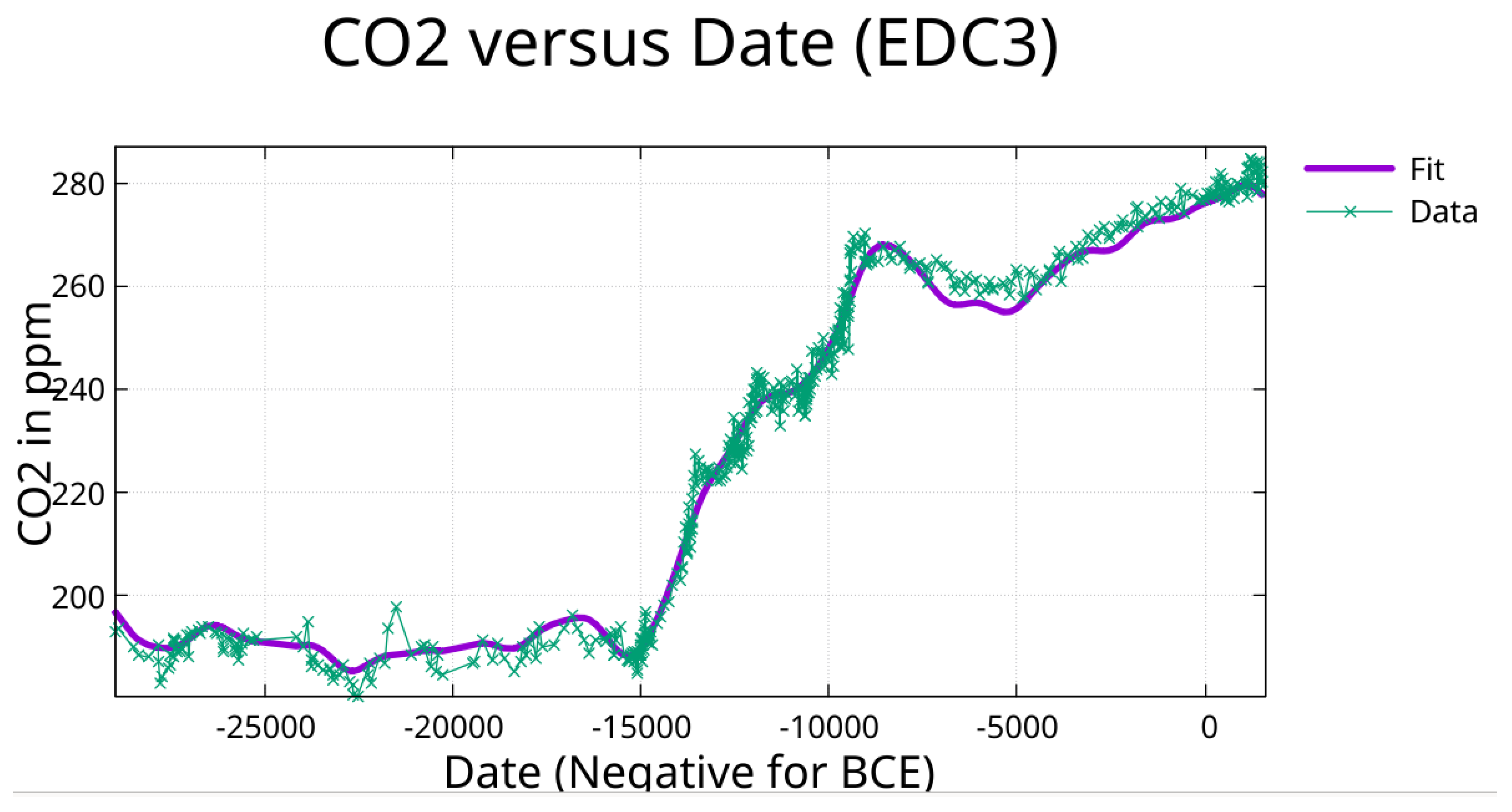
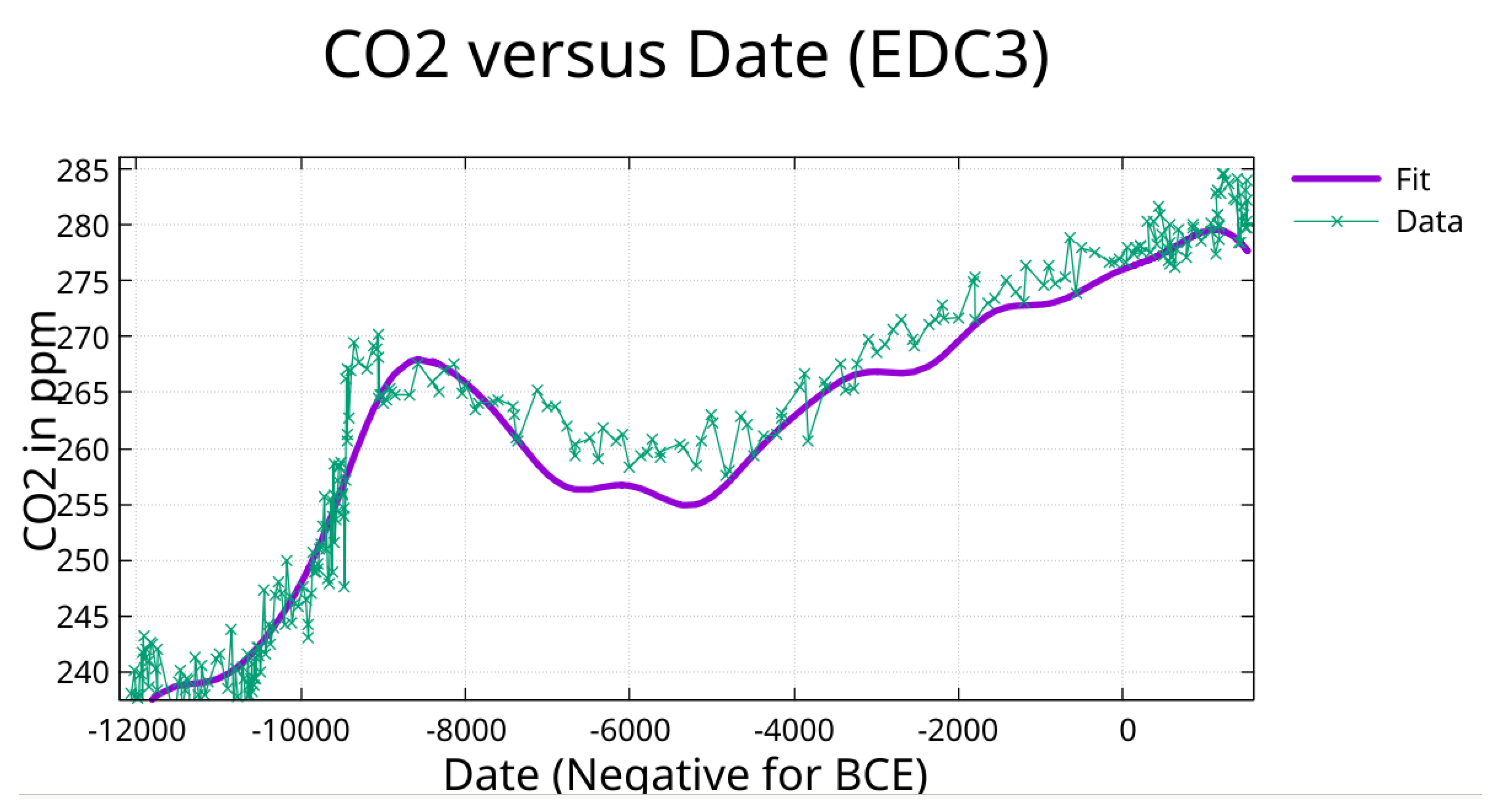
Figure 8.
Zoom on Figure 5 showing the fit from date -12,000 to date 1515. There is an obvious separation of the fit from the data for the last 10,000 years for this case that is not in the fit where periods are found independently.
Figure 8.
Zoom on Figure 5 showing the fit from date -12,000 to date 1515. There is an obvious separation of the fit from the data for the last 10,000 years for this case that is not in the fit where periods are found independently.
3.2. Recovery of Milankovitch Periods
The algorithm independently recovered periods matching canonical Milankovitch cycles (Milankovitch, 1941):
| Recovered Period (yr) | Canonical Cycle | Physical Origin |
| 113,600 | ~100,000 | Eccentricity |
| 40,200 | ~41,000 | Obliquity |
| 23,000 | ~23,000 | Precession |
3.3. CO₂ Fit Using Periods from Temperature Fit and Phase Analysis
The CO₂ fit, using periods from the temperature fit, achieves R² = 0.964. For phase comparison, amplitudes were normalized to positive values (adding 180° to phase when amplitude was negative). Phase lag = (Δφ/360°) × P, with negative values indicating CO₂ lagging temperature. See Supplementary Table S4 for fit parameters.
The fit of CO₂ data to the same periods was done: (1) to determine if the same periods would fit the CO₂ data, (2) to allow direct comparison of phase for each period.
A fit of CO₂ data using the greedy algorithm with pruning will be presented and discussed below.
3.4. Phase Lag Results with Uncertainties Where Both Fits Use the Same Periods
The table presents two standard error estimates reflecting different assumptions about phase constraints. SE₁ assumes temperature phase is constrained by orbital forcing theory, treating only the CO₂ phase as uncertain. Under this assumption, the eccentricity lag (−4,853 yr) differs from zero at 3.3σ, while obliquity and precession lags are marginally significant at 1.5σ and 1.9σ respectively.
SE₂ incorporates uncertainty in both phases from the empirical fits. These larger values—often exceeding the lag estimates themselves—reflect the genuine difficulty of determining phases from relatively weak orbital-frequency signals in a noisy record. Using SE₂, no individual period achieves conventional statistical significance.
The evidential weight therefore comes not from individual periods but from the collective pattern: five of six dominant periods show CO₂ lagging temperature, with a mean lag of −1,688 years. Under a null hypothesis of zero systematic lag, this consistency is unlikely to arise by chance. However, we emphasize that this is pattern-level evidence rather than statistically significant determination of any individual lag value.
The large SE₂ values also quantify the “100,000-year problem”: temperature amplitudes at orbital frequencies are remarkably small (0.5–3°C), yet the late Pleistocene is dominated by ~100,000-year glacial cycles with 7–10°C swings. The eccentricity signal produces the weakest direct forcing yet appears to dominate. Whatever amplification mechanism transforms these subtle periodic forcings into dramatic climate oscillations, it operates with substantial noise or nonlinearity that limits precise phase determination.
The fit of CO₂ data using the greedy algorithm with pruning (46 periods), and a fit of the CH₄ data using the greedy algorithm with pruning are discussed below. The phase issue for these fits is addressed with cross-correlation.
3.5. The Eemian CO₂ Plateau
The Last Interglacial reveals profound asymmetry: from −130,000 to −117,000 years, temperature declined ~7°C while CO₂ remained at 275–280 ppm. This 13,000-year plateau indicates CO₂ absorption during cooling is much slower than release during warming.
This observation poses a fundamental challenge to interpretations where CO₂ serves as the primary amplifier of orbital forcing. At the Eemian peak (~127,000 BCE), all positive feedback mechanisms—CO₂, water vapor, reduced ice albedo—were presumably at maximum strength. If these feedbacks collectively amplify weak orbital forcing into major glacial-interglacial swings, what mechanism can overcome them to initiate cooling while CO₂ remains elevated? The 13,000-year duration excludes transient explanations; for comparison, the Younger Dryas lasted less than 2,000 years and the entire Holocene spans only 11,700 years.
The phase lag analysis (Table 2) compounds this puzzle. If CO₂ systematically lags temperature by 1,500–4,900 years at orbital frequencies, CO₂ responds to temperature rather than driving it. The Eemian plateau then becomes interpretable: CO₂ remained high because ocean uptake is slow, but its elevated concentration was insufficient to prevent cooling once some other factor initiated the temperature decline. The question of what initiates glacial inception while all greenhouse feedbacks are maximized remains open (Higginbotham, 2025).
3.6. Mid-Pleistocene Transition (MPT)
Consistent with the MPT (Clark et al., 2006; Berends et al., 2021), Figure 9 indicates that the periods that fit the data well from date -350,000 to 1911 are not appropriate for the temperature variations prior to date -400,000. The R squared value for this plot was 0.7.
Figure 9.
Here the full Temperature proxy data set was fit with the same 55 periods found by the temperature fit and a constant. The fit from date -400,000 to 1911 is fit reasonably well but the deviations for dates prior to date -400,000 are large. This is consistent with the MPT.
Figure 9.
Here the full Temperature proxy data set was fit with the same 55 periods found by the temperature fit and a constant. The fit from date -400,000 to 1911 is fit reasonably well but the deviations for dates prior to date -400,000 are large. This is consistent with the MPT.
The dominant ~100,000-year eccentricity cycle that characterizes the late Pleistocene is largely absent in the earlier record, which was dominated by the ~41,000-year obliquity cycle. The fit to the ~800,000 years of data using periods determined on data from date -350,000 and later appears to be almost orthogonal to the data prior to date -400,000.
Figure 10 shows how a running computation of R squared produces a sharp drop for this fit at date -400,000 (400,000 BCE). This running R² analysis also inherits the natural weighting from sampling density discussed in Section 2.3—degradation backward in time reflects both genuine fit failure at the MPT and the decreasing statistical leverage of increasingly sparse older data.
Figure 10.
Here the average squared deviation and the variance are computed from date 1911 into the past as running quantities. This allows the computation of R squared for the fit from a given horizontal axis date forward in time to 1911.
Figure 10.
Here the average squared deviation and the variance are computed from date 1911 into the past as running quantities. This allows the computation of R squared for the fit from a given horizontal axis date forward in time to 1911.
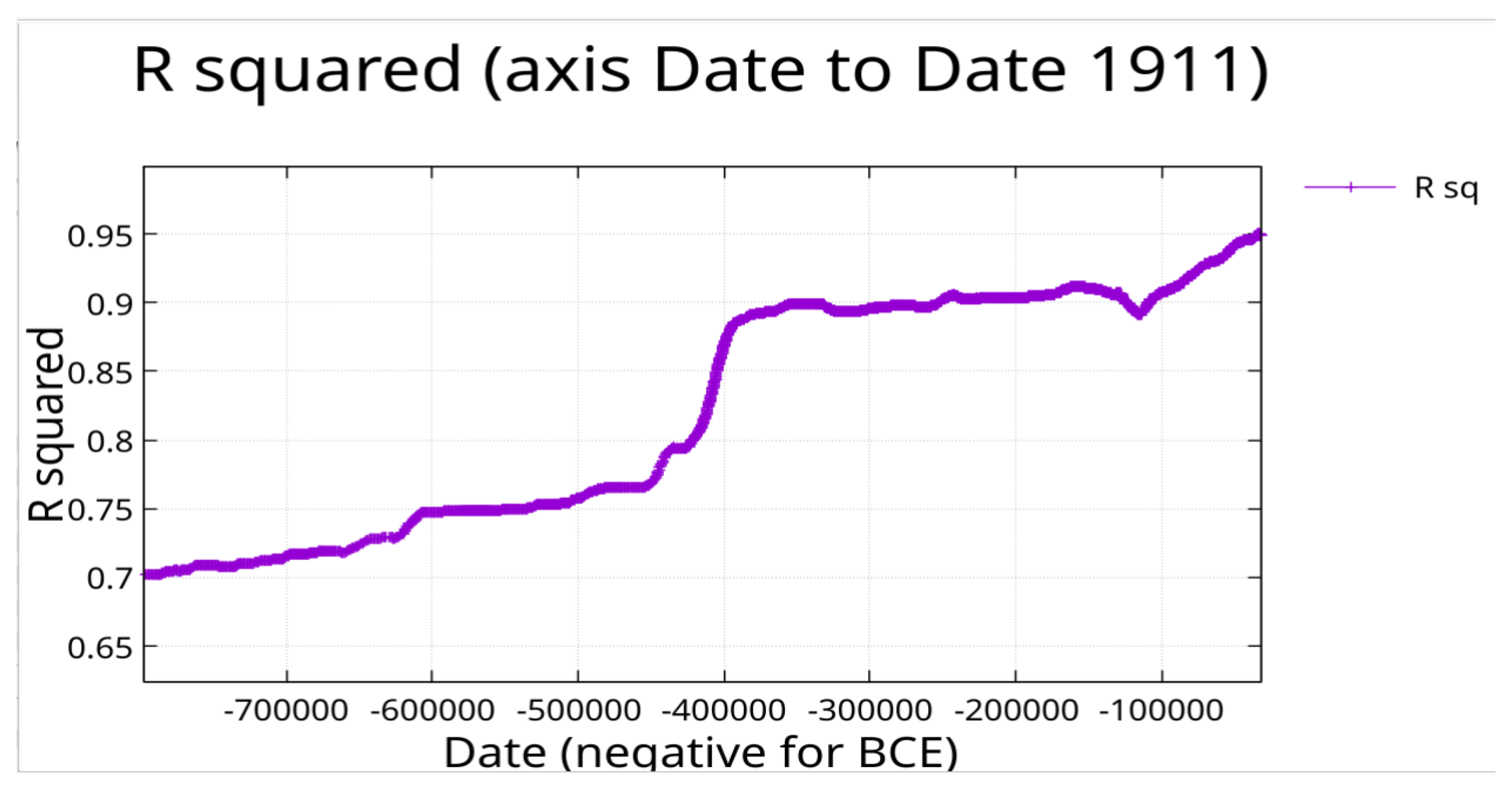
Figure 11.
CO₂ fit (EDC3 chronology, from date -350,000 to 1515) with periods found using the greedy algorithm followed by pruning to minimize off diagonal correlation.
Figure 11.
CO₂ fit (EDC3 chronology, from date -350,000 to 1515) with periods found using the greedy algorithm followed by pruning to minimize off diagonal correlation.
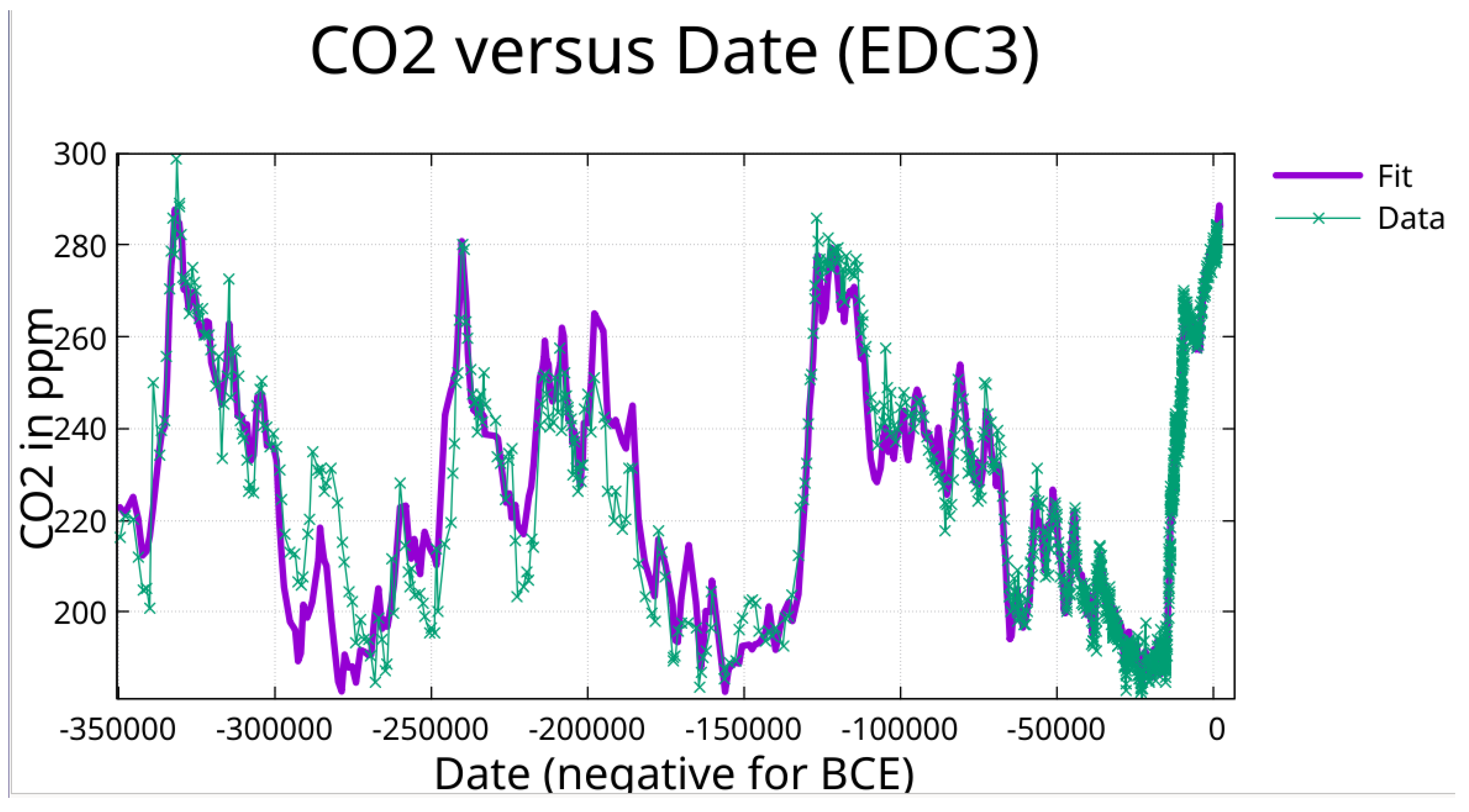
Figure 12.
Zoom on plot of greedy algorithm fit to CO₂ (EDC3 chronology).
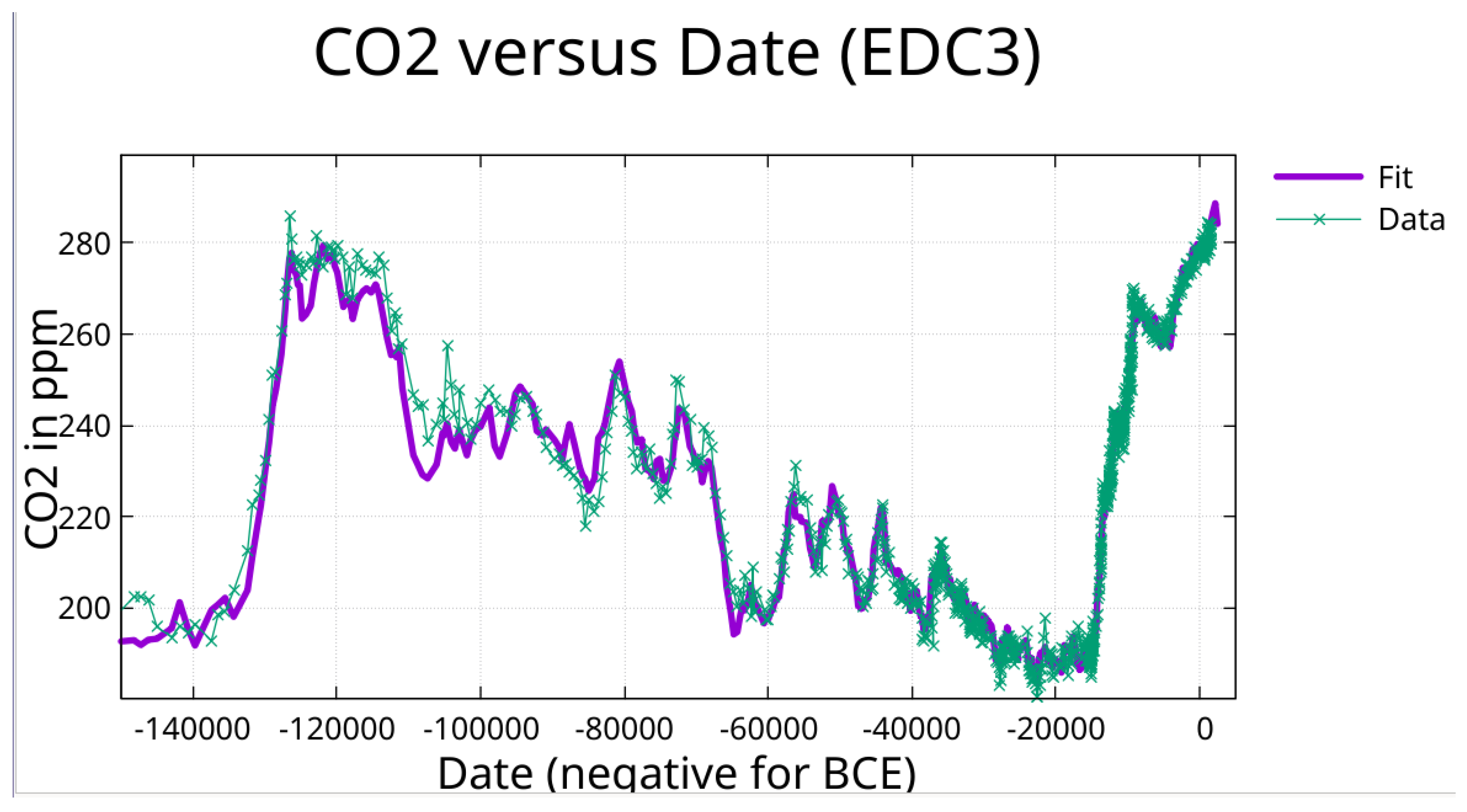
Figure 13.
Zoom on previous plot of greedy algorithm fit to CO₂.
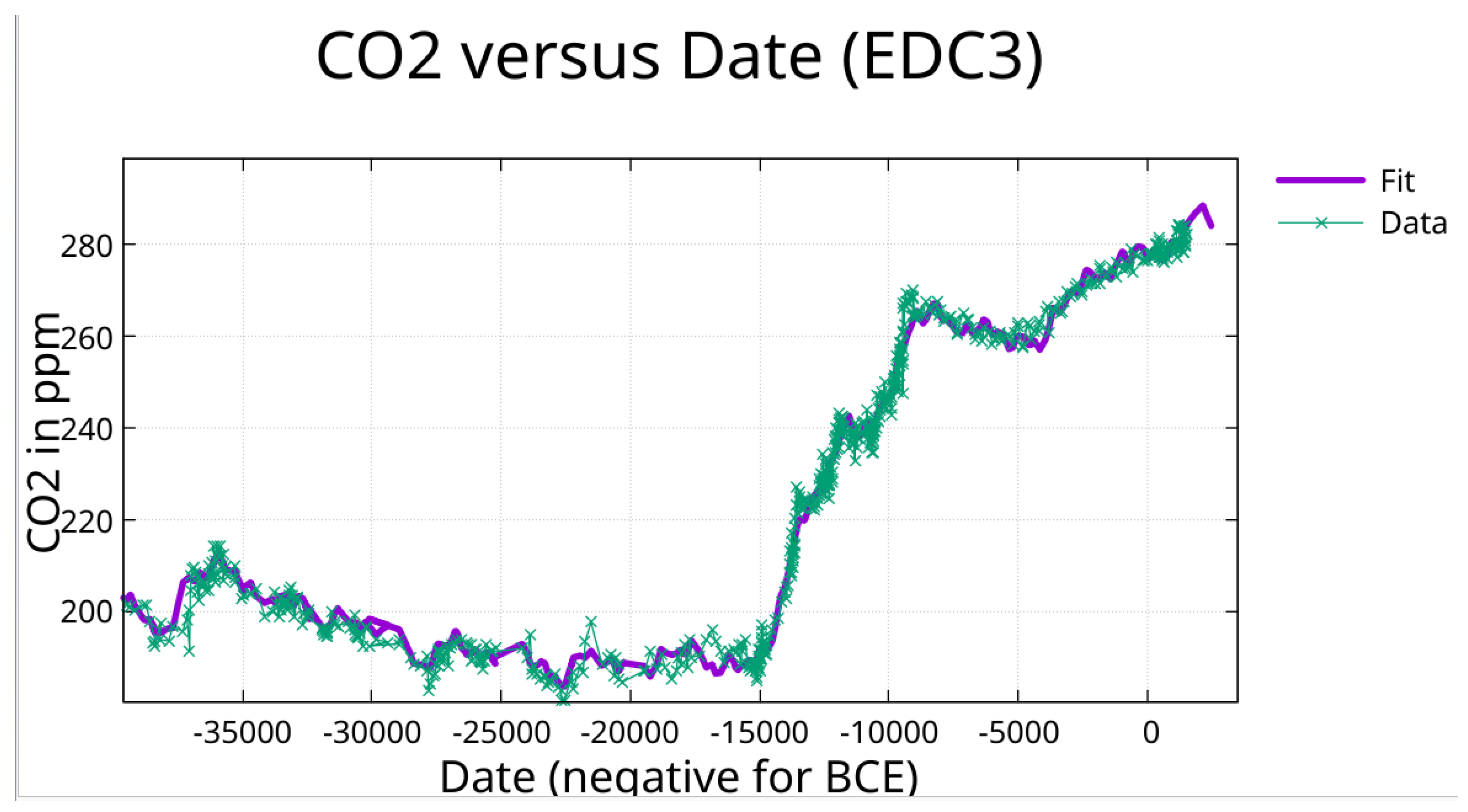
Figure 14.
Zoom on previous plot of greedy algorithm fit to CO₂.

3.7. CO₂ Fit with Periods from Greedy Algorithm
The CO₂ fit found by the greedy algorithm followed by pruning to minimize off diagonal correlation, achieves R² = 0.966 using a constant and 46 periods. The maximum off diagonal correlation is below 0.55. See Supplementary Table S6 for fit parameters.
3.8. CH₄ Fit with Periods from Greedy Algorithm
This independent recovery validates both the methodology and the orbital pacing hypothesis for glacial-interglacial cycles.
The greedy algorithm independently recovered orbital periods for all cases:
| Temperature | CO₂ | CH₄ | Canonical | |
| Eccentricity | 113,600 yr | 114,600 yr | 109,400 yr | ~100,000 yr |
| Obliquity | 40,200 yr | 40,350 yr | 40,100 yr | ~41,000 yr |
| Precession | 23,000 yr | 23,050 yr | 23,100 yr | ~23,000 yr |
See Supplementary Table S7 for CH₄ fit parameters.
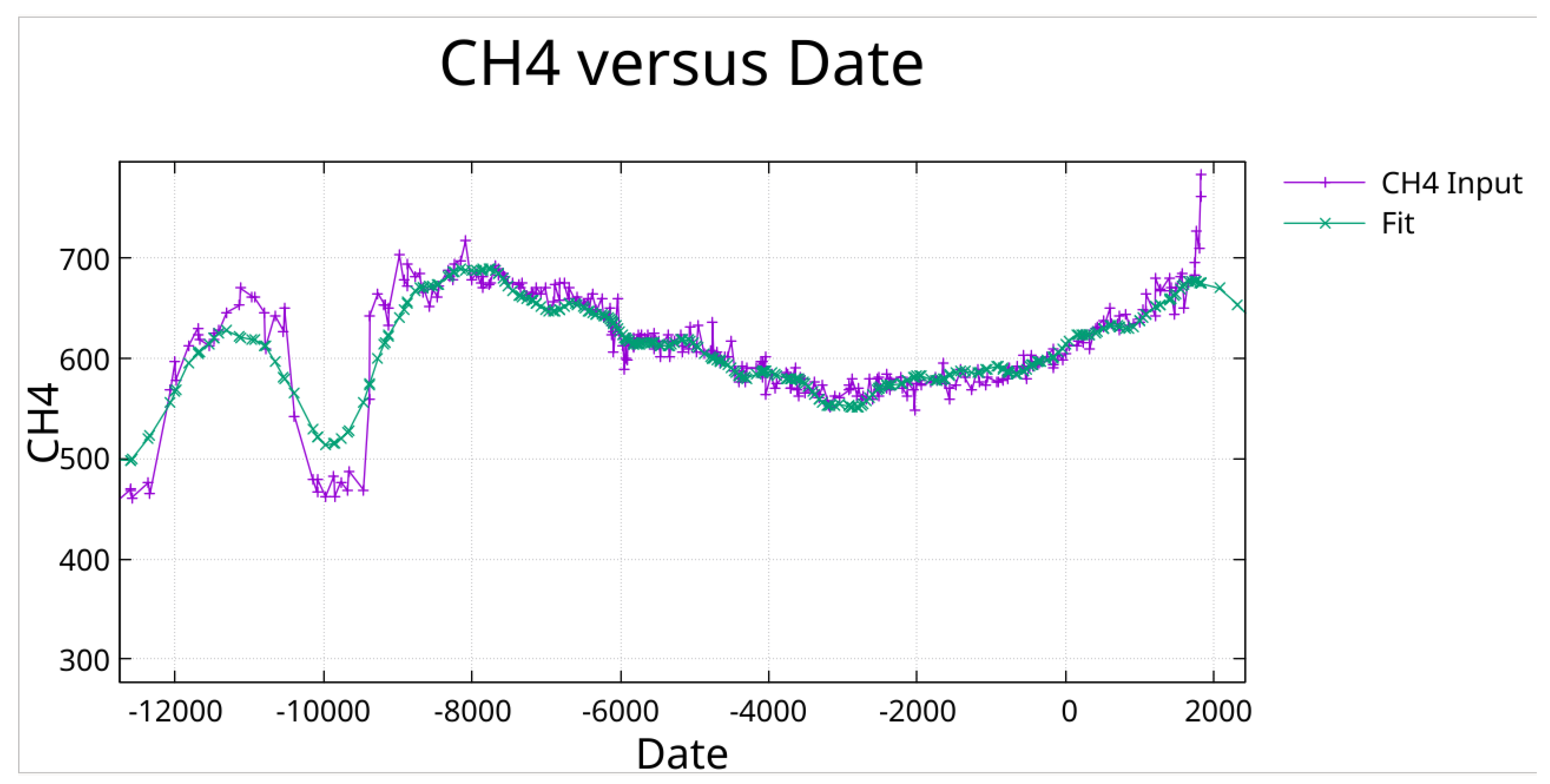
Figure 15.
CH₄ in ppb fit with periods found by greedy algorithm followed by pruning to minimize off diagonal correlation.
Figure 15.
CH₄ in ppb fit with periods found by greedy algorithm followed by pruning to minimize off diagonal correlation.
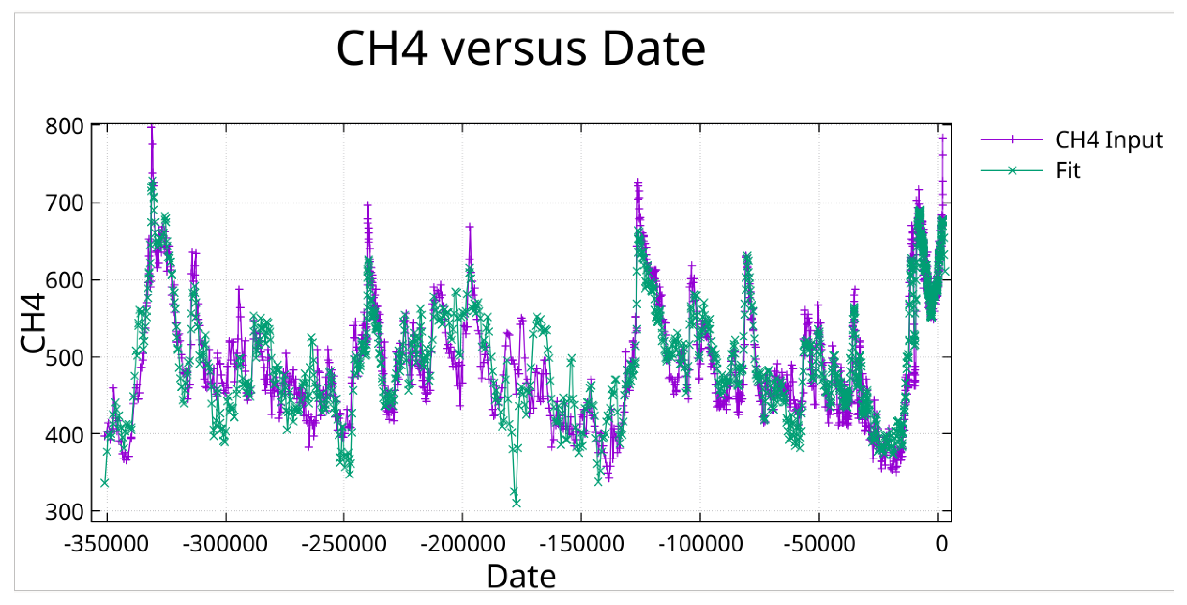
Figure 16.
Zoom on previous Figure.
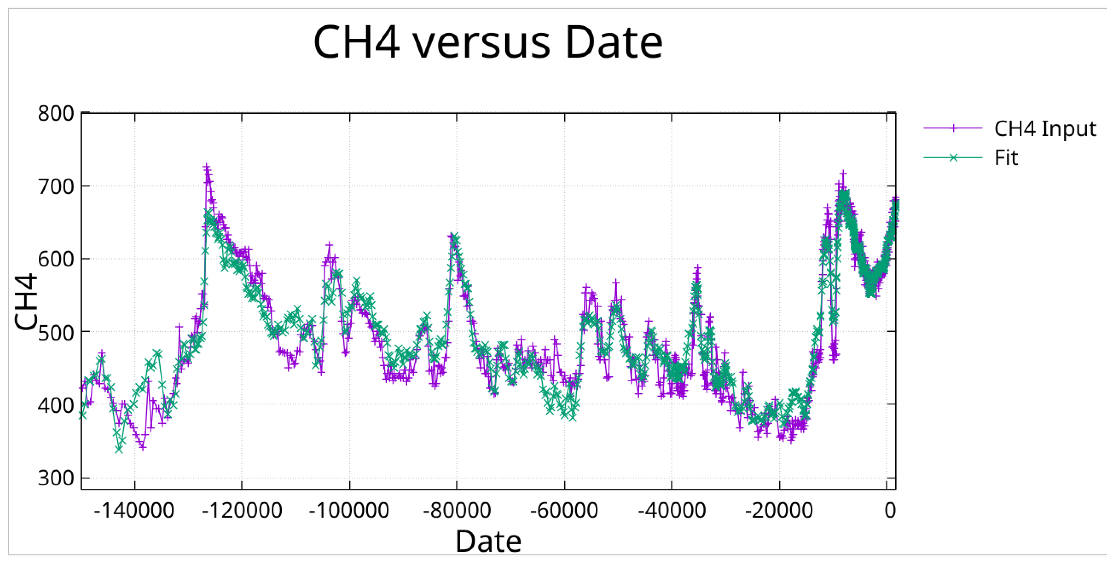
Figure 17.
Zoom on previous Figure. Note the fit to the Younger Dryas notch at around 10,000 BCE.
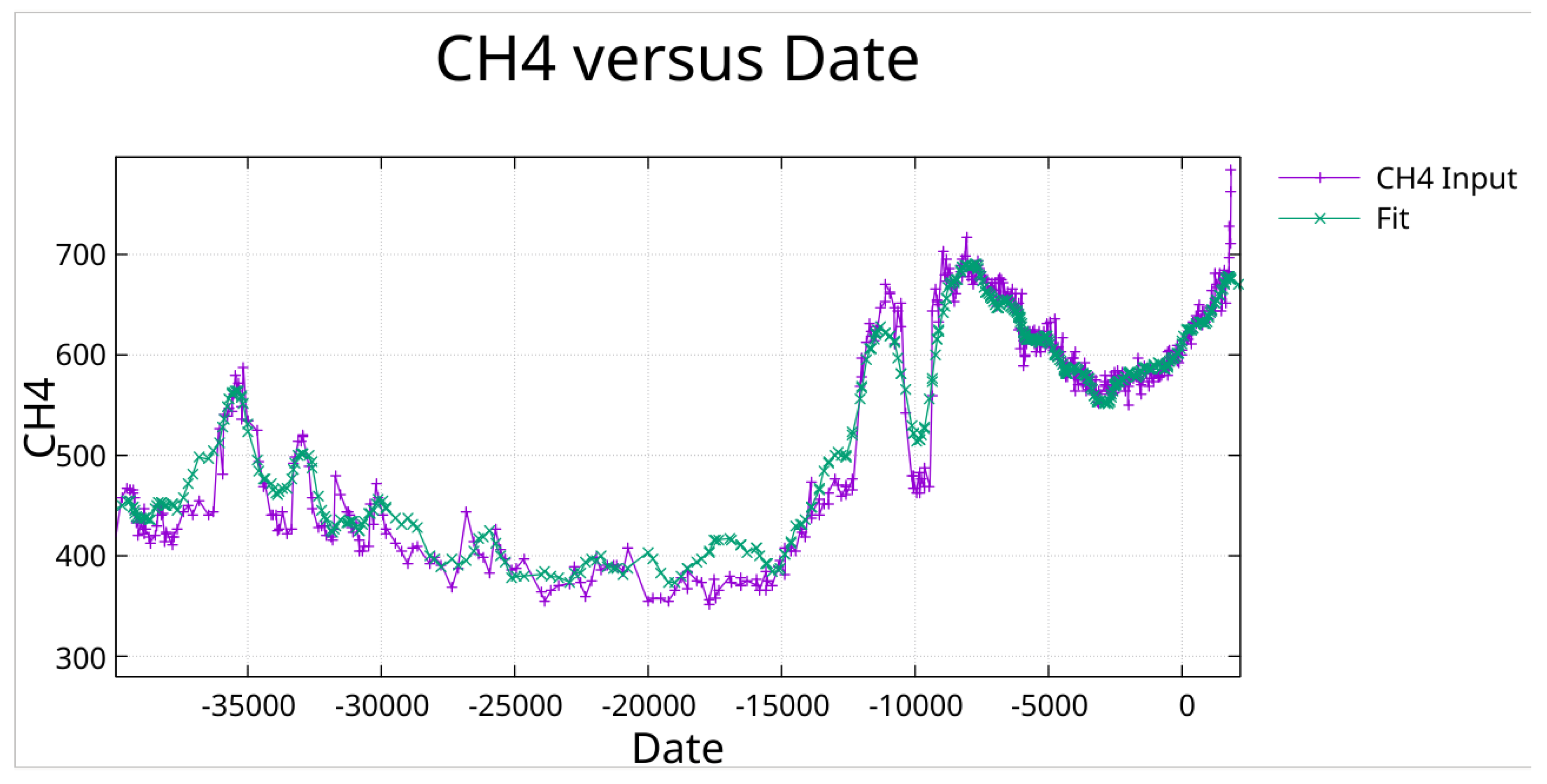
Figure 18.
Zoom on previous Figure showing more clearly the fit to the Younger Dryas.
3.9. Cross Correlation
The fit to temperature was evaluated at 10 year intervals from 350,000 BCE to 1850 CE. Similarly the fit to CO₂ by the greedy algorithm with pruning (46 periods and a constant) was similarly evaluated. These time series were cross correlated and the results are shown in Figure 19.
Cross-correlation was computed as a function of time lag τ, where positive τ represents CO₂/CH₄ shifted forward relative to temperature – a positive lag. A peak in correlation at negative lag indicates that the second variable (CO₂ or CH₄) follows temperature; a peak at positive lag would indicate the reverse. The correlation values shown are negative because the fits were evaluated relative to their respective means, and both gases increase with warming (positive correlation with temperature change from the mean).
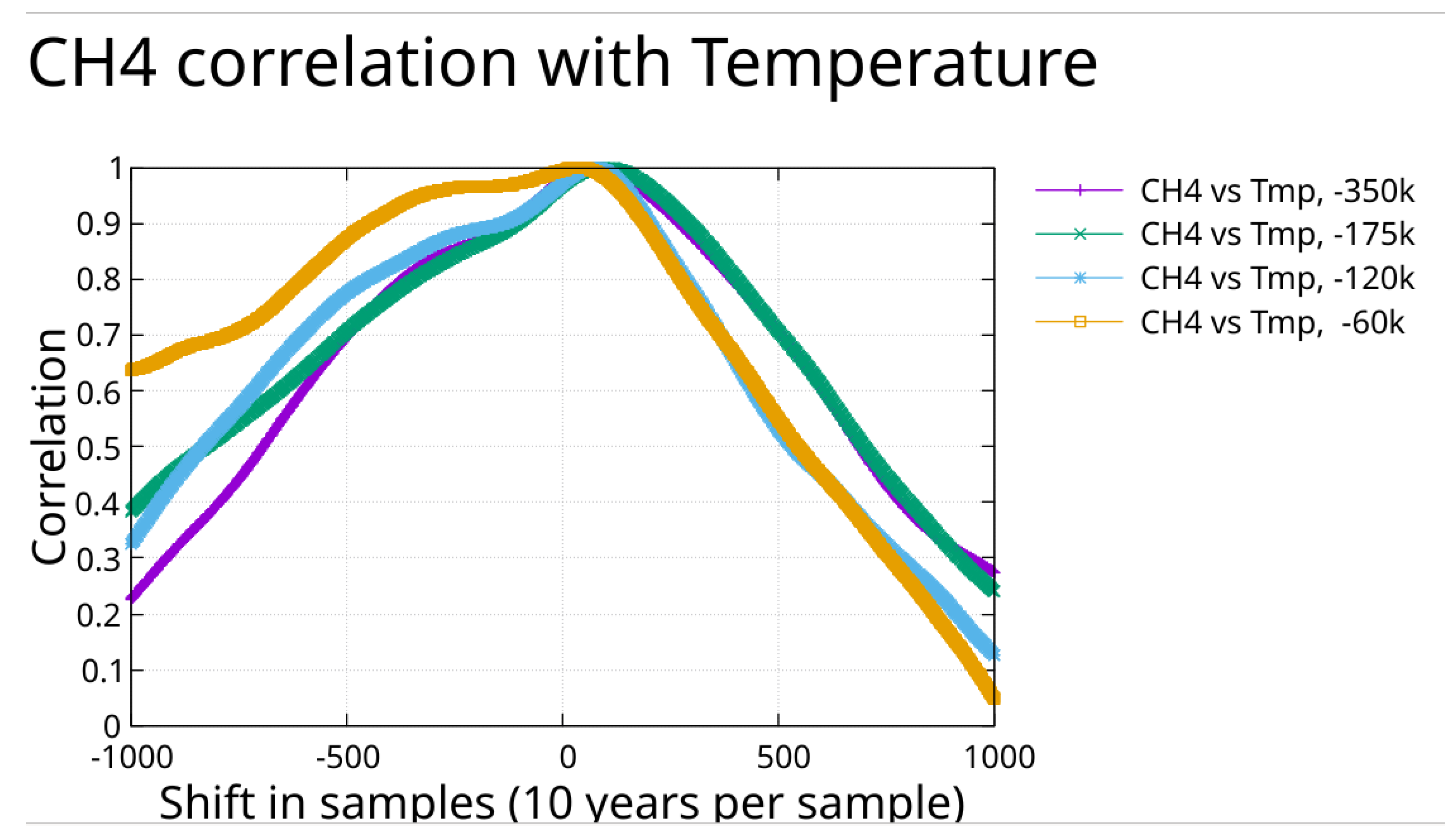
Similarly the fit to CH₄ was evaluated and cross correlated with temperature. For all cases plotted, CH₄ shows a lag with respect to temperature.
The consistency of the lag for CH₄ indicates that the time series agree on registration of their respective quantity with time.
The cross-correlation results reveal a systematic dependence on the time interval analyzed. For the full 350,000-year record, the correlation peak occurs at negative lag (CO₂ following temperature). As the analysis window is progressively restricted toward recent times, the peak shift approaches zero and, for the 60,000-year interval, shows a broad plateau suggesting near-synchronous or slightly positive lag behavior.
It is perhaps worth noting here that when the temperature with EDC3 chronology was correlated with the CO₂ on AICC2012 chronology, the CO₂ showed a ~2000 year lag for the 352,000 year interval, a ~300 year lag for the 177,000 year interval, a 500 year lead for the 122,000 year interval, and a ~1000 year lead for the 62,000 year interval with all intervals ending at year 1850.
Two interpretations merit consideration. First, the Eemian CO₂ plateau—where CO₂ remained elevated for ~13,000 years while temperature declined—may dominate the longer intervals, creating an apparent lag that reflects asymmetric response kinetics rather than a simple phase relationship. The shorter intervals exclude or underweight this asymmetric feature. Second, systematic chronology drift between the temperature and CO₂ records cannot be excluded; if such drift increases with age, it would manifest as interval-dependent lag shifts. The CH₄-temperature cross-correlation shows consistent lag behavior across all intervals, suggesting the chronological alignment of temperature and CH₄ (both on EDC3) is more reliable than the converted record.
These results underscore that the phase relationship between temperature and CO₂ is not a simple constant but depends on timescale and possibly on the specific climate transitions included in the analysis interval.
Figure 19.
The times series for temperature and CO₂ (EDC3) for intervals, 350,000 BCE -1515 CE, 175,000 BCE – 1515 CE, 120,000 BCE – 1515 CE, and 60,000 BCE – 1515 CE, were cross correlated. The results are plotted here showing a lag in CO₂ except for a broad plateau with a lead in the most recent time interval.
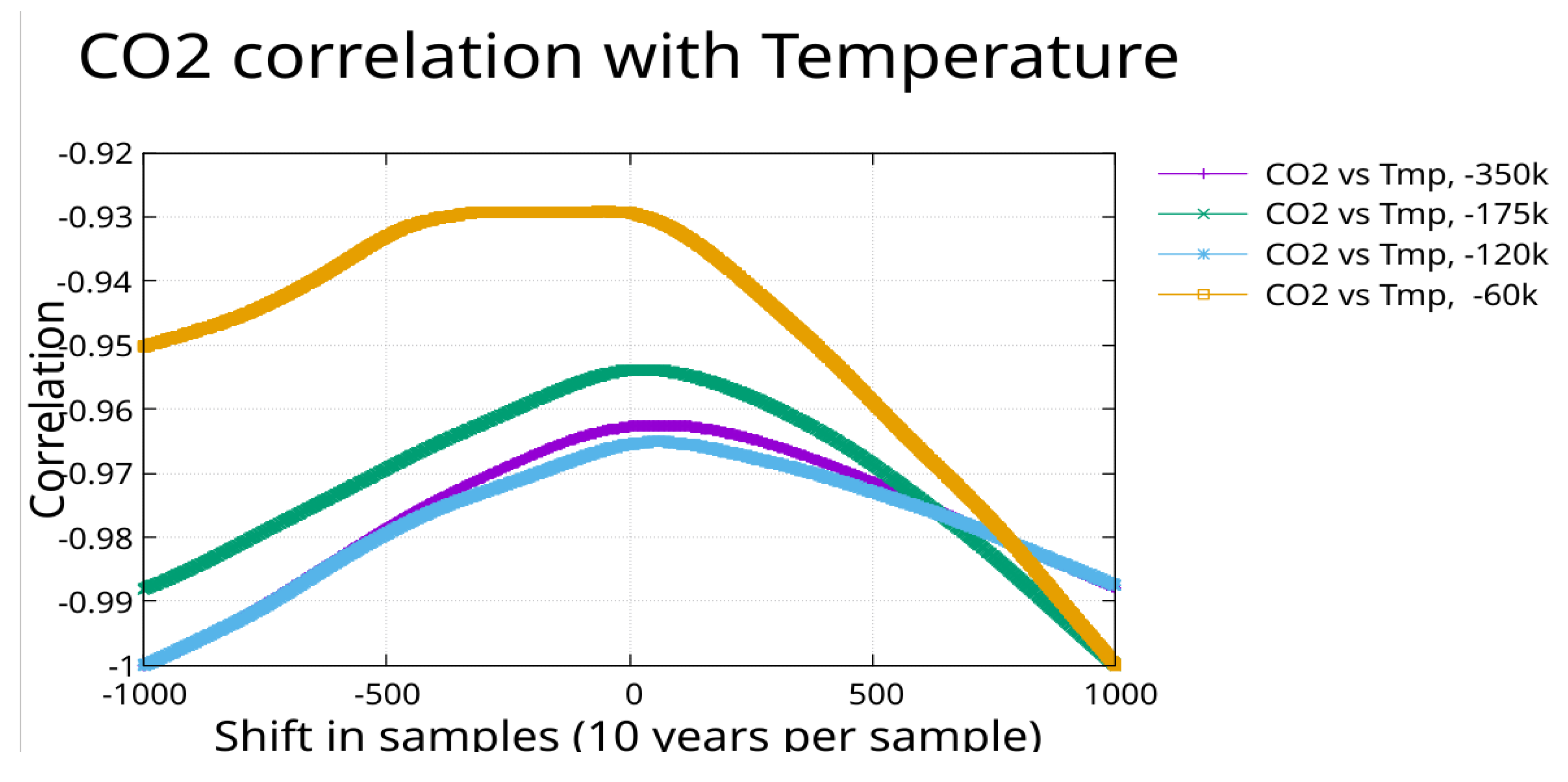
Figure 20.
The times series for temperature and CH₄ for intervals, 350,000 BCE -1850 CE, 175,000 BCE – 1850 CE, 120,000 BCE – 1850 CE, and 60,000 BCE – 1850 CE, were cross correlated. All cases show a lag with respect to temperature.
Figure 20.
The times series for temperature and CH₄ for intervals, 350,000 BCE -1850 CE, 175,000 BCE – 1850 CE, 120,000 BCE – 1850 CE, and 60,000 BCE – 1850 CE, were cross correlated. All cases show a lag with respect to temperature.
3.10. Cross Plots
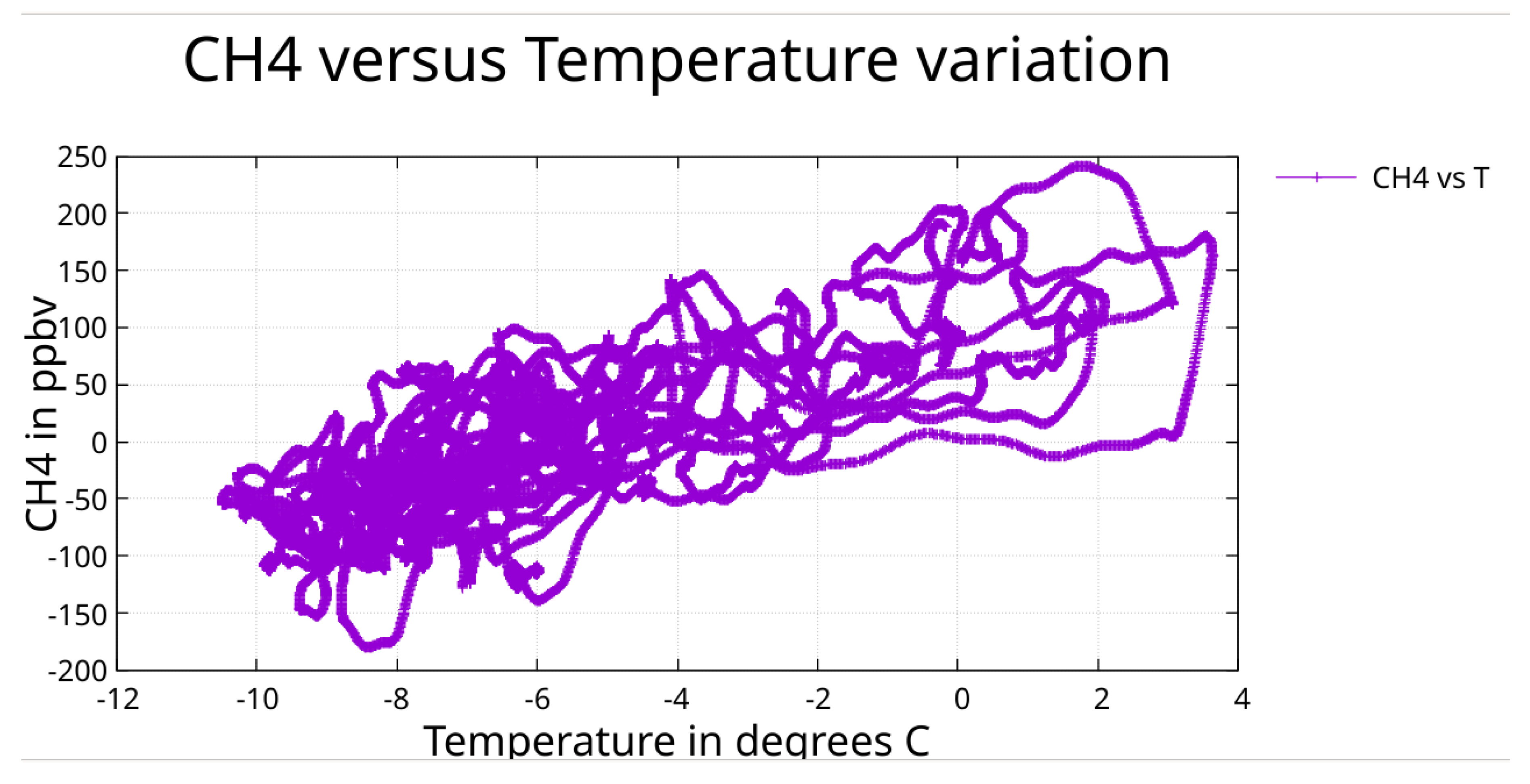
The time series used for the correlations of Section 3.9 were used to generate cross plots. The cross plot for CO₂ indicates a curvature that tends toward flattening with higher temperature. This may have an influence on the asymmetry discussed in Section 3.5. The CH₄ cross plot shows a linear trend. High temperatures are associated with the relatively narrow interglacial peaks. This limits the data available at high temperatures in these plots.
This saturation behavior of CO₂ is consistent with temperature-dependent ocean solubility, where the capacity for CO₂ release diminishes as the ocean warms.
The linear CH₄-temperature relationship in cross-plot analysis (Figure 22) contrasts with the hysteresis evident in cross-correlation, suggesting, but not proving, that CH₄ variability arises from source heterogeneity (wetlands, permafrost, clathrates) rather than from nonlinear temperature response.
Figure 21.
Here CO₂ (EDC3) is plotted against temperature. This plot shows curvature that tends to flatten as the temperature rises.
Figure 21.
Here CO₂ (EDC3) is plotted against temperature. This plot shows curvature that tends to flatten as the temperature rises.
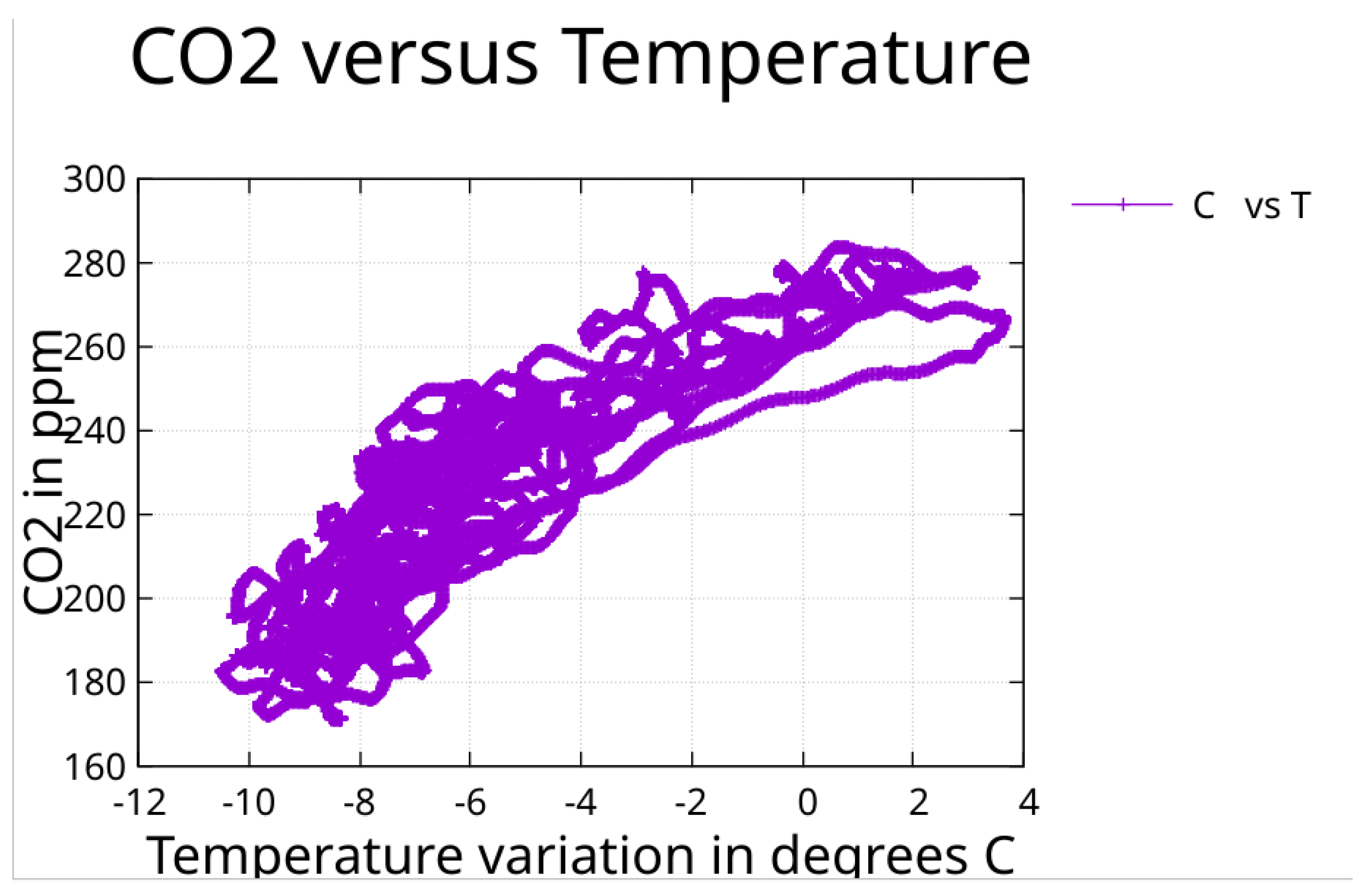
Figure 22.
Here CH₄ is plotted against temperature showing a linear trend.
3.11. Temperature Fit over the Last Glacial Cycle
The 135,000-year temperature fit with 2-year period search steps achieves R² = 0.960, slightly exceeding the 350,000-year fit (R² = 0.952) while covering a complete glacial cycle including the Eemian interglacial peak. With eccentricity (113,600 yr) and obliquity (40,200 yr) fixed, the greedy algorithm independently recovered a precession-related period at 22,974 yr, consistent with the canonical ~23,000-year cycle.
The finer 2-year search steps allow detection of periods that may be missed with coarser stepping. Notable periods recovered include 69,840 yr (related to eccentricity modulation), 29,650 yr, and numerous millennial-scale periods. Sub-millennial periods down to 952 yr provide resolution of recent climate features including the Little Ice Age. The fit demonstrates that harmonic analysis remains effective over a single glacial cycle when the longest periods are appropriately constrained, achieving comparable or better R² than the full 350,000-year analysis with fewer periods (33 versus 55).
See Supplementary Table S8 for the complete parameter list.
Figure 23.
Fit from date -135,000 to date 1911 with a constant and 33 periods or one period for every 4000 years of input data.
Figure 23.
Fit from date -135,000 to date 1911 with a constant and 33 periods or one period for every 4000 years of input data.
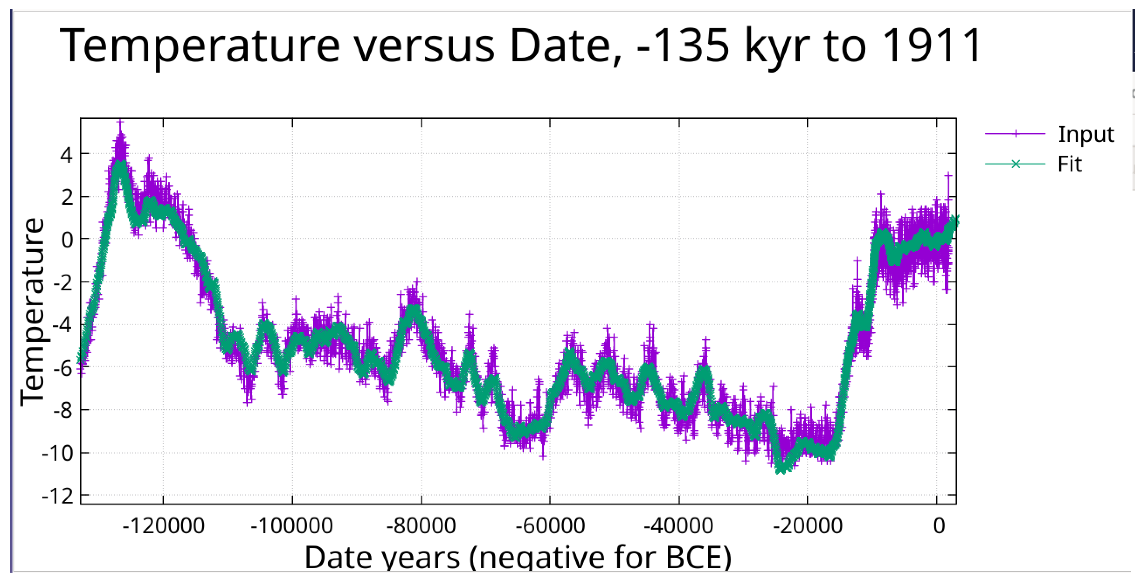
Figure 24.
Zoom showing the fit from date -40,000 to 1911.
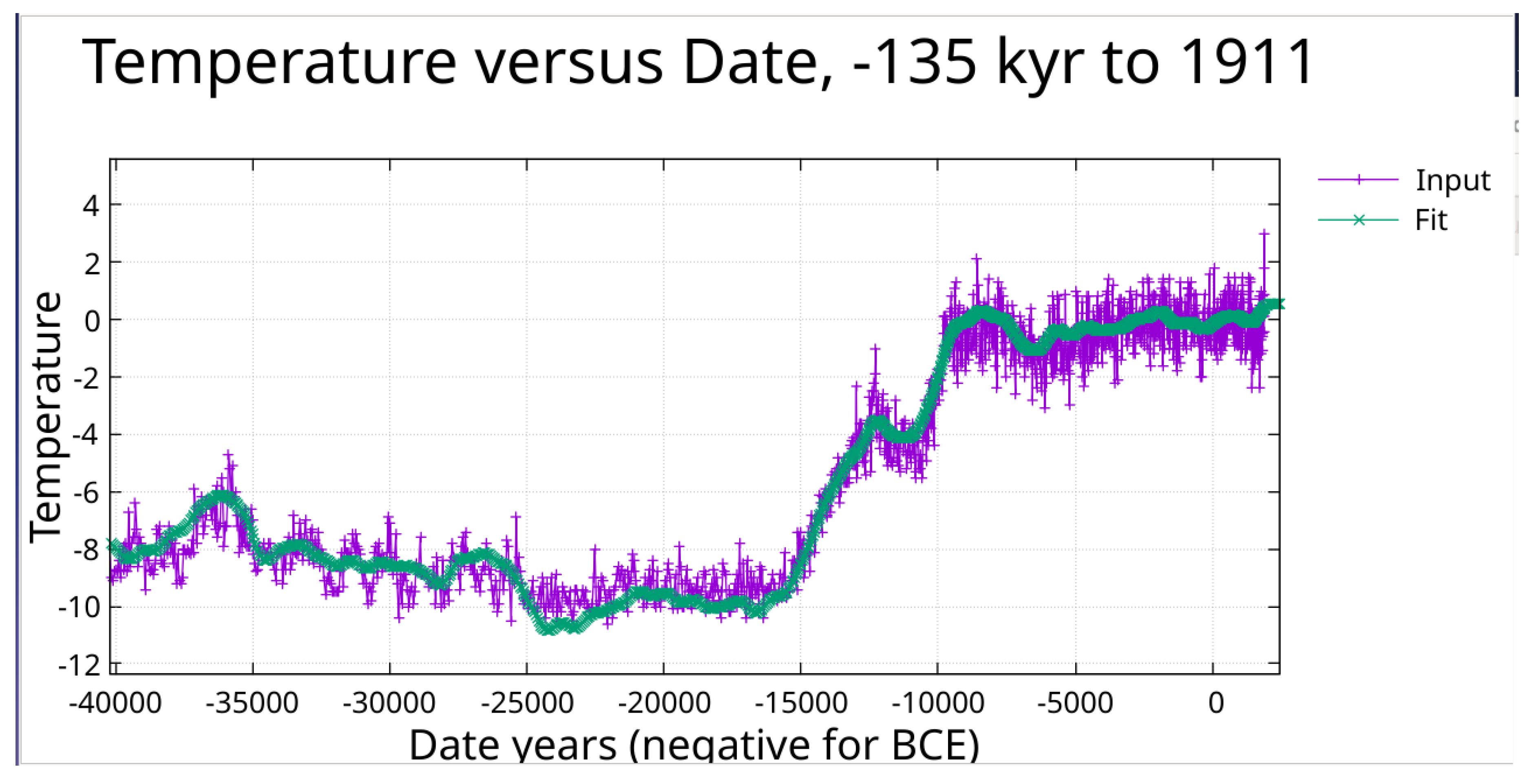
Figure 25.
Zoom showing the fit from the Younger Dryas event to date 1911.
4. Discussion
4.1. Temperature Drives CO₂ at Orbital Timescales
The pattern of CO₂ lagging temperature at orbital periods, observed when both variables are fit with the same harmonic components, is consistent with a model where temperature changes precede CO₂ changes. Both variables fit with R² > 0.95, and the systematic negative lag across major Milankovitch periods suggests a physical relationship rather than fitting artifact.
This pattern supports an interpretation where: (1) orbital forcing modulates insolation; (2) temperature responds; (3) CO₂ responds to temperature through ocean degassing, circulation changes, and terrestrial carbon storage. Such an interpretation is consistent with previous phase analyses (Humlum et al., 2013; Grabyan, 2025) and with the physical chemistry of CO₂ ocean-atmosphere exchange.
However, several caveats apply. The individual phase determinations carry large uncertainties (Table 2, SE₂). The cross-correlation analysis shows interval-dependent behavior, with recent intervals showing near-zero or positive lag. And the Eemian plateau demonstrates that the CO₂-temperature relationship involves asymmetric dynamics that simple phase analysis may not fully capture. The evidence is more consistent with temperature-driven CO₂ variation than with CO₂-driven temperature variation at orbital timescales, but the relationship is clearly more complex than a simple constant lag.
It is difficult to explain a mechanism that would cause CO₂ to rise and fall with a periodic structure. To get the “orbital clock” involved as a mechanism, it has to first cause a warming which then releases CO₂ – the warming comes first. Similarly, if the warming comes first then that warming should also support higher sustained levels of water vapor in the atmosphere without a prerequisite CO₂ rise. This “mechanism” argument, together with the phase and correlation findings of these calculations, may be the strongest argument that CO₂ does indeed lag temperature.
The independent recovery of Milankovitch periods by the greedy algorithm, without prior specification, validates that these signals are genuine features of the data. The consistency across temperature, CO₂, and CH₄ records further supports the orbital pacing hypothesis.
4.2. Mechanisms for Asymmetric Response
Atmospheric Transport Limitation: During warming, dissolved CO₂ is immediately available for release at the air-sea interface. During cooling, atmospheric CO₂ must find its way back to the ocean surface—a rate-limited process.
Plant Stress Feedback: As CO₂ declines, C3 vegetation becomes stressed near 200 ppm, reducing uptake and creating a floor below which CO₂ cannot easily fall.
Sea Ice Expansion: Growing sea ice caps the ocean surface, reducing gas exchange area precisely when cooling is most rapid.
4.3. The Modern CO₂ Anomaly
The fit extrapolated beyond the data shows gentle Holocene oscillation around 270–280 ppm. Actual CO₂ departing above 350 ppm after ~1850 CE lies far outside the orbital envelope. This analysis establishes the baseline from natural forcing; whatever drives modern CO₂, it is not the orbital mechanics governing the past 350,000 years.
4.4. Alternative Amplification Mechanisms
The combination of weak orbital temperature signals (reflected in large SE₂ values), systematic CO₂ lag, and the Eemian plateau invites consideration of alternative amplification mechanisms. Water vapor is the dominant greenhouse gas, contributing more radiative forcing than CO₂. The standard interpretation holds that CO₂ warming triggers water vapor increase, which amplifies the warming. However, warming from any source—including direct orbital forcing—should increase both CO₂ and water vapor simultaneously. There is no physical requirement that CO₂ increase must precede water vapor increase.
If water vapor responds directly to orbital-driven warming (bypassing CO₂ as intermediary), then both CO₂ and water vapor become parallel responses to temperature rather than sequential links in a causal chain. This reframing has implications for glacial inception: rising water vapor eventually triggers increased cloud formation, and clouds exert net cooling through albedo effects. Once cloud-driven cooling begins, it may persist even as CO₂ remains elevated—potentially explaining the Eemian plateau.
This conjecture faces significant challenges: we have no water vapor measurements from the Eemian, and the relationship between atmospheric water vapor and cloud formation is complex and not fully understood. Nevertheless, the difficulty climate models have with glacial inception (Vavrus et al., 2018; Willeit et al., 2024) suggests that current understanding of the feedback mechanisms governing interglacial-to-glacial transitions remains incomplete. The quantitative evidence presented here—CO₂ lagging temperature, weak orbital amplitudes, and the Eemian anomaly—warrants continued investigation of alternative mechanisms (Higginbotham, 2025).
5. Conclusions
- Greedy harmonic analysis fits Antarctic ice core temperature, CO₂ and CH₄ over 350,000 years with R² > 0.95, independently recovering Milankovitch periods (Milankovitch, 1941). Covariance matrix analysis guided refinement of the temperature fit, in particular, from 59 to 55 periods, ensuring stable parameter estimates. The refinement from 59 to 55 periods eliminated all correlations exceeding |r| = 0.50, reducing the maximum from 0.95 to 0.15 for temperature.
- Phase analysis reveals a pattern of CO₂ lagging temperature at the major Milankovitch periods. Five of six dominant orbital periods show negative lags with a mean of approximately −1,700 years. While individual lag determinations carry large uncertainties, the systematic pattern supports an interpretation where temperature changes precede CO₂ changes at orbital timescales. Cross-correlation analysis corroborates this for longer intervals but shows interval-dependent behavior that warrants further investigation. The physical mechanism associated with the “orbital clock” essentially requires that temperature rise first to thereby release CO2 into the atmosphere.
- The Eemian shows CO₂ elevated for ~13,000 years while temperature fell ~7°C, indicating asymmetric absorption/release kinetics. This asymmetric behavior may be the reason direct comparison of phase is difficult.
- The modern CO₂ spike is anomalous relative to the 350,000-year orbital pattern – obvious for all existing ice-core data.
- The Younger Dryas temperature event is fit quite well as can be seen in Figure 4. The fit involves 111 fit parameters but this corresponds to roughly one parameter every 3000 years which seems quite reasonable for the observed accuracy of the fit, especially given the normalized covariance indication of little correlation between periods. The Younger Dryas event is even more prominent in the CH₄ data and is harder to fit but it is reasonably well represented as shown in Figure 18.
- The R squared analysis shown in Figure 10 appears to unambiguously find the Mid-Pleistocene Transition and clearly justifies limiting the fit to the interval chosen.
Supplementary Materials
The following supporting information can be downloaded at the website of this paper posted on Preprints.org.
Funding
No external funding was received for this research.
Conflicts of interest
The author declares no conflicts of interest.
References
- Bazin, L., Landais, A., Lemieux-Dudon, B., Toyé Mahamadou Kele, H., Veres, D., Parrenin, F., Martinerie, P., Ritz, C., Capron, E., Lipenkov, V., Loutre, M.-F., Raynaud, D., Vinther, B., Svensson, A., Rasmussen, S.O., Severi, M., Blunier, T., Leuenberger, M., Fischer, H., Masson-Delmotte, V., Chappellaz, J., & Wolff, E. (2013). An optimized multi-proxy, multi-site Antarctic ice and gas orbital chronology (AICC2012): 120–800 ka. Climate of the Past, 9, 1715–1731. [CrossRef]
- Bereiter, B., Eggleston, S., Schmitt, J., Nehrbass-Ahles, C., Stocker, T.F., Fischer, H., Kipfstuhl, S., & Chappellaz, J. (2015). Revision of the EPICA Dome C CO₂ record from 800 to 600 kyr before present. Geophysical Research Letters, 42, 542–549. [CrossRef]
- Berends, C.J., Köhler, P., Lourens, L.J., & van de Wal, R.S.W. (2021). On the Cause of the Mid-Pleistocene Transition. Reviews of Geophysics, 59, e2020RG000727. [CrossRef]
- Bouchet, M., Landais, A., Grisart, A., Parrenin, F., Prié, F., Jacob, R., Fourré, E., Capron, E., Raynaud, D., Lipenkov, V.Ya., Loutre, M.-F., Extier, T., Svensson, A., Legrain, E., Martinerie, P., Leuenberger, M., Jiang, W., Ritterbusch, F., Lu, Z.-T., & Yang, G.-M. (2023). The Antarctic Ice Core Chronology 2023 (AICC2023) chronological framework and associated timescale for the European Project for Ice Coring in Antarctica (EPICA) Dome C ice core. Climate of the Past, 19, 2257–2286. [CrossRef]
- Clark, P.U., Archer, D., Pollard, D., Blum, J.D., Rial, J.A., Brovkin, V., Mix, A.C., Pisias, N.G., & Roy, M. (2006). The middle Pleistocene transition: characteristics, mechanisms, and implications for long-term changes in atmospheric pCO₂. Quaternary Science Reviews, 25, 3150–3184. [CrossRef]
- Grabyan, R. (2025). Global Atmospheric CO₂ Lags Temperature: Implications for Short- and Long-Term Climate Predictions. Science of Climate Change, 5(3), 302–326.
- Higginbotham, J. (2025 a). Planetary Orbits and Sea-Level During the Phanerozoic: Correlation, Causation, and Forecasting. Journal of Biomedical Research & Environmental Sciences, 6(4), 926–940.
- Humlum, O., Stordahl, K., & Solheim, J.E. (2013). The phase relation between atmospheric carbon dioxide and global temperature. Global and Planetary Change, 100, 51–69. [CrossRef]
- Higginbotham, J. (2025 b). Climate, Water Vapor, and Volcanic Eruptions. Preprints.org. [CrossRef]
- Jouzel, J., et al. (2007). Orbital and Millennial Antarctic Climate Variability over the Past 800,000 Years. Science, 317(5839), 793–796. [CrossRef]
- Loulergue, L., Schilt, A., Spahni, R., Masson-Delmotte, V., Blunier, T., Lemieux, B., Barnola, J.-M., Raynaud, D., Stocker, T.F., & Chappellaz, J. (2008). Orbital and millennial-scale features of atmospheric CH₄ over the past 800,000 years. Nature, 453, 383–386. [CrossRef]
- Milankovitch, M. (1941). Kanon der Erdbestrahlung und seine Anwendung auf das Eiszeitenproblem. Royal Serbian Academy Special Publication 133, Belgrade.
- Parrenin, F., Barnola, J.-M., Beer, J., Blunier, T., Castellano, E., Chappellaz, J., Dreyfus, G., Fischer, H., Fujita, S., Jouzel, J., Kawamura, K., Lemieux-Dudon, B., Loulergue, L., Masson-Delmotte, V., Narcisi, B., Petit, J.-R., Raisbeck, G., Raynaud, D., Ruth, U., Schwander, J., Severi, M., Spahni, R., Steffensen, J.P., Svensson, A., Udisti, R., Waelbroeck, C., & Wolff, E. (2007). The EDC3 chronology for the EPICA Dome C ice core. Climate of the Past, 3, 485–497. [CrossRef]
- Veres, D., Bazin, L., Landais, A., Toyé Mahamadou Kele, H., Lemieux-Dudon, B., Parrenin, F., Martinerie, P., Blayo, E., Blunier, T., Capron, E., Chappellaz, J., Rasmussen, S.O., Severi, M., Svensson, A., Vinther, B., & Wolff, E.W. (2013). The Antarctic ice core chronology (AICC2012): an optimized multi-parameter and multi-site dating approach for the last 120 thousand years. Climate of the Past, 9, 1733–1748. [CrossRef]
- Vavrus, S.J., He, F., Kutzbach, J.E., Ruddiman, W.F., & Tzedakis, P.C. (2018). Glacial Inception in Marine Isotope Stage 19: An Orbital Analog for a Natural Holocene Climate. Scientific Reports, 8, 10213. [CrossRef]
- Willeit, M., Calov, R., Talento, S., Greve, R., Bernales, J., Klemann, V., Bagge, M., & Ganopolski, A. (2024). Glacial inception through rapid ice area increase driven by albedo and vegetation feedbacks. Climate of the Past, 20, 597–623. [CrossRef]
Table 2.
Phase relationships for dominant periods (55-period fit, EDC3 chronology).
| Period (yr) | T Phase (°) | CO₂ Phase (°) | Lag (yr) | SE₁ (yr) | SE₂ (yr) | Cycle |
| 113,600 | 233.6 | 218.2 | −4,853 | 1,486 | 9,997 | Eccentricity |
| 40,200 | 343.0 | 327.3 | −1,757 | 1,196 | 5,059 | Obliquity |
| 65,000 | 158.7 | 147.6 | −2,002 | 2,076 | 13,200 | — |
| 23,000 | 357.7 | 332.9 | −1,584 | 854 | 5,486 | Precession |
| 29,600 | 156.2 | 175.8 | +1,611 | 1,808 | 8,628 | — |
| 26,600 | 152.6 | 131.8 | −1,540 | 3,841 | 13,822 | — |
Notes: Phases normalized to positive amplitude convention. Negative lag indicates CO₂ lags temperature. SE₁ uses CO₂ phase uncertainty only (appropriate if temperature phase is constrained by orbital theory); SE₂ uses both CO₂ and temperature phase uncertainties from covariance matrix diagonal elements via error propagation.
Disclaimer/Publisher’s Note: The statements, opinions and data contained in all publications are solely those of the individual author(s) and contributor(s) and not of MDPI and/or the editor(s). MDPI and/or the editor(s) disclaim responsibility for any injury to people or property resulting from any ideas, methods, instructions or products referred to in the content. |
© 2025 by the author. Licensee MDPI, Basel, Switzerland. This article is an open access article distributed under the terms and conditions of the Creative Commons Attribution (CC BY) license (http://creativecommons.org/licenses/by/4.0/).
Copyright: This open access article is published under a Creative Commons CC BY 4.0 license, which permit the free download, distribution, and reuse, provided that the author and preprint are cited in any reuse.


