
Submitted:
02 December 2025
Posted:
03 December 2025
You are already at the latest version
Abstract
To enhance desalination efficiency and reduce experimental costs, the development of advanced mathematical models for EMS is essential. In this study, we propose a novel hybrid approach that integrates neural networks with high-accuracy numerical simulations of electroconvection. Based on dimensionless similarity criteria (Reynolds, Péclet numbers, etc.), we establish functional relationships between critical parameters, such as the dimensionless electroconvective vortex diameter and the plateau length of current-voltage curves. Training datasets were generated through extensive numerical experiments using our in-house developed mathematical model, while multilayer feedforward neural networks with backpropagation optimization were employed for regression tasks. The resulting AI (artificial intelligence) -driven hybrid models enable rapid prediction and optimization of EMS design and operating parameters, reducing computational and experimental costs. This research is situated at the intersection of membrane science, artificial intelligence, and computational modeling, forming part of a broader foresight agenda aimed at developing next-generation intelligent membranes and adaptive control strategies for sustainable water treatment. The proposed methodology offers a scalable framework for integrating physics-informed modeling and machine learning into the design of high-performance electromembrane systems.
Keywords:
1. Introduction
- 1)
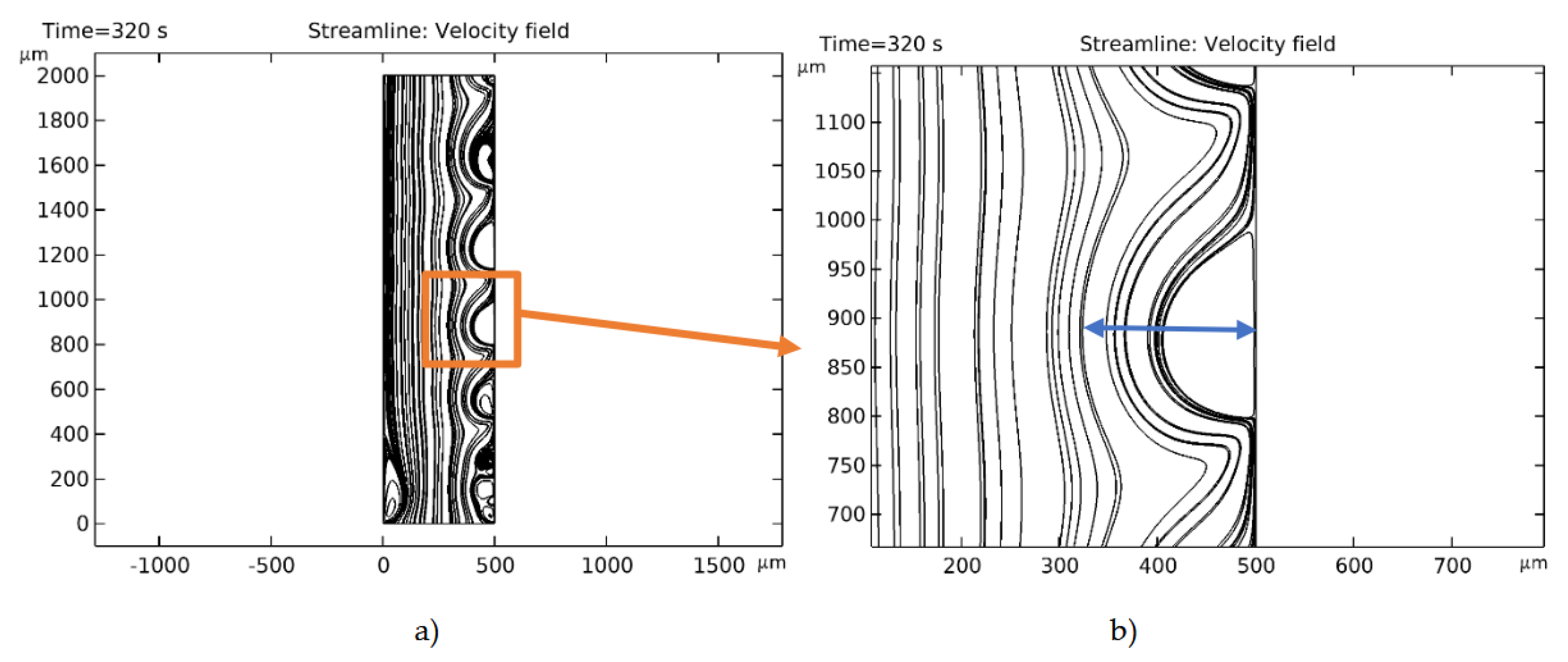
- in the potentiostatic case we have (using the example of the dimensionless diameter of an electroconvective vortex Decv):
2. Methods
2.1. Mathematical Model
2.2. Similarity Method for Transport Processes in a Flat Channel
3. Results
3.1. Training Set for Constructing a Neural Network
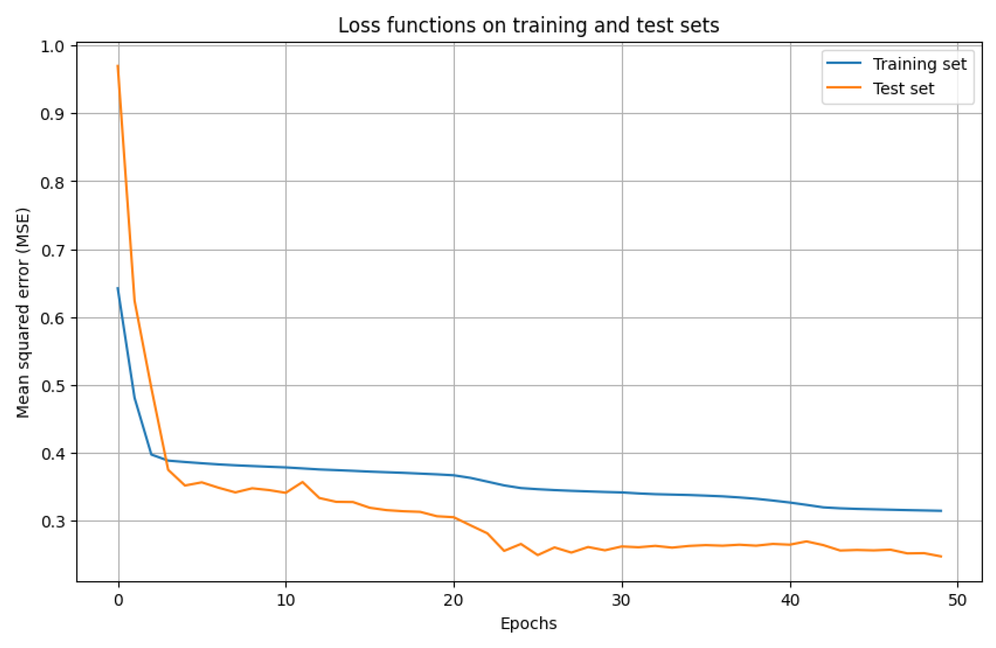
3.2. Building a Neural Network
4. Discussion
Author Contributions
Funding
Data Availability Statement
Conflicts of Interest
Abbreviations
| CEM | Cation exchange membrane |
| AEM | Anion exchange membrane |
| ECV | Electroconvective vortex |
| EMS | Electromembrane systems |
| DC | Desalination channel |
| CVC | Current voltage characteristic |
| ANN | Artificial neural networks |
| AI | Artificial intelligence |
References
- Abuwatfa, W.H.; AlSawaftah, N.; Darwish, N.; Pitt, W.G.; Husseini, G.A. A Review on Membrane Fouling Prediction Using Artificial Neural Networks (ANNs). Membranes 2023, 13, 685. [CrossRef]
- Jawad, J.; Hawari, A.H.; Zaidi, S.J. Modeling and Sensitivity Analysis of the Forward Osmosis Process to Predict Membrane Flux Using a Novel Combination of Neural Network and Response Surface Methodology Techniques. Membranes 2021, 11, 70. [CrossRef]
- Di Martino, M.; Abraham, E.J.; Pistikopoulos, E.N.; et al. A Neural Network Based Superstructure Optimization Approach to Reverse Osmosis Desalination Plants. Membranes 2022, 12, 199. [CrossRef]
- Galinha, C.F.; Crespo, J.G. From Black Box to Machine Learning: A Journey through Membrane Process Modelling. Membranes 2021, 11, 574. [CrossRef]
- Recent Advances in the Prediction of Fouling in Membrane Bioreactors. Membranes 2021, 11, 381. [CrossRef]
- Chengxin Niu; Bin Li, Zhiwei Wang. Using artificial intelligence-based algorithms to identify critical fouling factors and predict fouling behavior in anaerobic membrane bioreactors, Journal of Membrane Science, Volume 687, 2023, 122076, ISSN 0376-7388. [CrossRef]
- Jiahui Hu; Changsu Kim; Peter Halasz; Jeong F. Kim; Jiyong Kim; Gyorgy Szekely. Artificial intelligence for performance prediction of organic solvent nanofiltration membranes, Journal of Membrane Science, Volume 619, 2021, 118513, ISSN 0376-7388. [CrossRef]
- Xintong Wang; Xin Sun; Youbing Wu; Feng Gao; Yu Yang. Optimizing reverse osmosis desalination from brackish waters: Predictive approach employing response surface methodology and artificial neural network models, Journal of Membrane Science, Volume 704, 2024, 122883, ISSN 0376-7388. [CrossRef]
- Heng Li; Bin Zeng; Jiayi Tuo; Yunkun Wang; Guo-Ping Sheng; Yunqian Wang. Development of an improved deep network model as a general technique for thin film nanocomposite reverse osmosis membrane simulation, Journal of Membrane Science, Volume 692, 2024, 122320, ISSN 0376-7388. [CrossRef]
- Fu-Heng Zhai; Qing-Qing Zhan; Yun-Fei Yang; Ni-Ya Ye; Rui-Ying Wan; Jin Wang; Shuai Chen; Rong-Huan He. A deep learning protocol for analyzing and predicting ionic conductivity of anion exchange membranes, Journal of Membrane Science, Volume 642, 2022, 119983, ISSN 0376-7388. [CrossRef]
- Gukhman, A.A. Introduction to Similarity Theory. Stereotype Publ. Publisher: LKI. – 2018. – 296 p.
- Grafov, B.M.; Chernenko, A.A. Theory of Direct Current Flow through a Binary Electrolyte Solution // Reports of the USSR Academy of Sciences. – 1962. Vol. 146. No. 1. Pp. 135-138.
- Grafov, B.M.; Chernenko, A.A. Direct Current Flow through a Binary Electrolyte Solution // Russian Journal of Physical Chemistry. – 1963. Vol. 37. Pp. 664.
- Urtenov M.K.; Uzdenova A.M.; Kovalenko A.V.; Nikonenko V.V.; Pismenskaya N.D.; Vasil’eva V.I.; Sistat P.; Pourcelly G. Basic mathematical model of overlimiting transfer in electrodialysis membrane systems enhanced by electroconvection // Journal Membrane Science 2013. V. 447. P. 190.
- Kovalenko A.V.; Nikonenko V.V.; Uzdenova A.M.; Urtenov M.Kh. Criterial numbers of electroconvection in the desalination chamber of an electrodialyzer // Condensed media and interphase boundaries: scientific journal. - No. 3 (16). Voronezh FGBOU HPE “Voronezh State University” 2013. P. 386-394.
- V.S. Pham; Z. Li; K.M. Lim; J.K. White, J. Han, Direct numerical simulation of electroconvective instability and hysteretic current-voltage response of a permselective membrane, Phys. Rev. E - Stat. Nonlinear Soft Matter Phys. 86 (2012) 046310. [CrossRef]
- Kirillova, E.; Kovalenko, A.; Urtenov, M. Study of the Current–Voltage Characteristics of Membrane Systems Using Neural Networks. AppliedMath 2025, 5, 10. [CrossRef]
 ) and cation (
 ), H — channel width, L — channel length.
) and cation (), H — channel width, L — channel length.
), H — channel width, L — channel length.
) and cation (), H — channel width, L — channel length.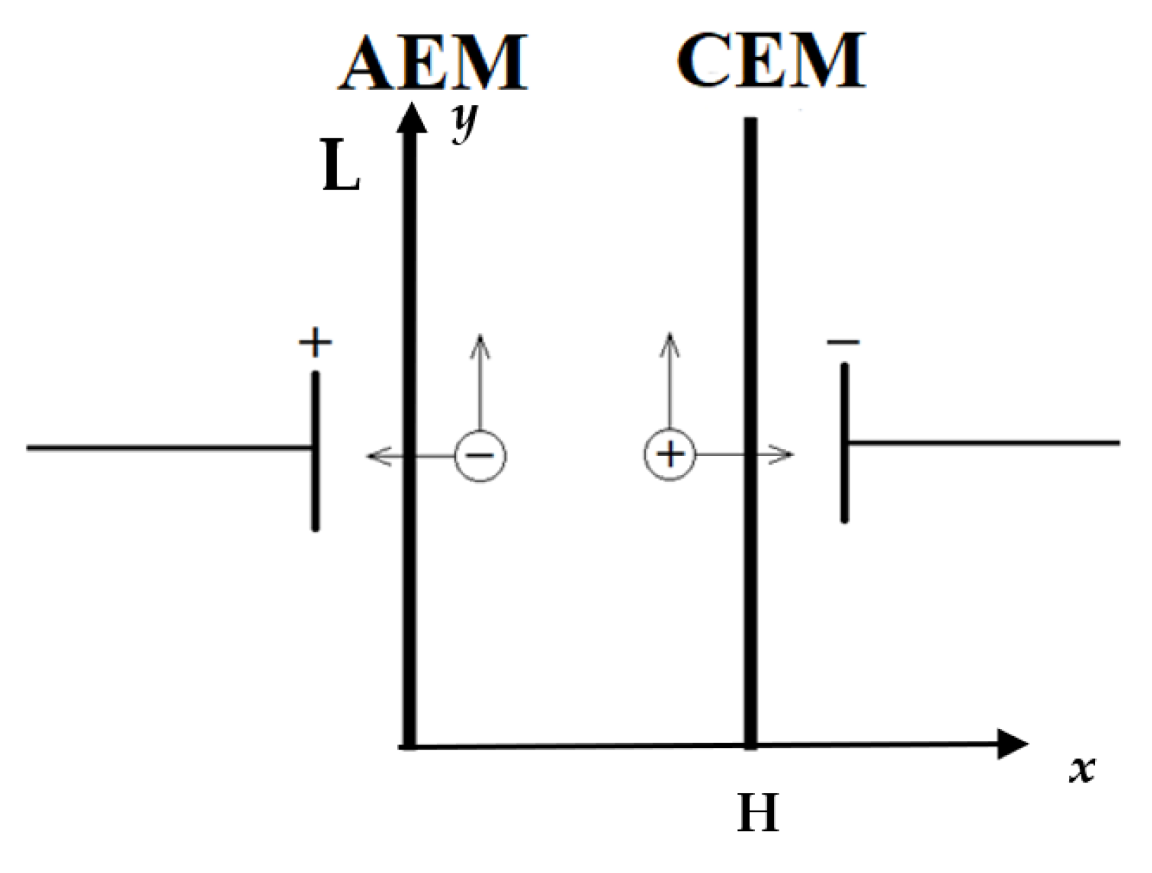

| № | d1 | Decv | Lpl | ECVCEM | ECVAEM |
|---|---|---|---|---|---|
| 1. | 0,01 | 0,342 | 17,29 | 25,42 | 49,19 |
| 2. | 0,04 | 0,334 | 17,46 | 25,5 | 49,57 |
| 3. | 0,05 | 0,334 | 17,54 | 25,3 | 48,7 |
| 4. | 0,06 | 0,35 | 17,79 | 25,67 | 49,22 |
| 5. | 0,07 | 0,326 | 17,99 | 25,77 | 49,08 |
| 6. | 0,09 | 0,318 | 17,62 | 25,86 | 50,09 |
| 7. | 0,11 | 0,346 | 17,96 | 26,05 | 49,58 |
| 8. | 0,12 | 0,32 | 17,85 | 25,83 | 49,95 |
| 9. | 0,13 | 0,318 | 16,85 | 25,97 | 49,94 |
| 10. | 0,15 | 0,32 | 17,72 | 26,13 | 50,21 |
| 11. | 0,16 | 0,324 | 17,61 | 25,85 | 50,9 |
| 12. | 0,17 | 0,328 | 17,64 | 25,74 | 48,75 |
| 13. | 0,18 | 0,33 | 17,54 | 26,34 | 48,29 |
| 14. | 0,19 | 0,32 | 17,12 | 24,13 | 46,7 |
| 15. | 0,21 | 0,324 | 17,7 | 26,2 | 48,89 |
| 16. | 0,24 | 0,35 | 16,97 | 25,5 | 49,28 |
| 17. | 0,39 | 0,354 | 7,192 | 23,35 | 47,48 |
| 18. | 0,49 | 0,33 | 6,97 | 26,271 | 49,14 |
| № | d1 | Re | Pe | Kel | Decv | Lpl | ECVCEM | ECVAEM |
|---|---|---|---|---|---|---|---|---|
| 1. | 0,01 | 0,05 | 24,39 | 2470000 | 0,342 | 17,29 | 25,42 | 49,19 |
| 2. | 0,01 | 0,1 | 48,78 | 619000 | 0,24 | 15,55 | 26,77 | 52,03 |
| 3. | 0,04 | 0,05 | 24,39 | 2470000 | 0,334 | 17,46 | 25,5 | 49,57 |
| 4. | 0,04 | 0,5 | 243,9 | 24700 | 0,114 | 11,44 | 30,88 | 56,41 |
| 5. | 0,04 | 0,1 | 48,78 | 619000 | 0,22 | 15,19 | 25,98 | 50,63 |
| 6. | 0,06 | 0,05 | 24,39 | 2470000 | 0,35 | 17,79 | 25,67 | 49,22 |
| 7. | 0,06 | 0,5 | 243,9 | 24700 | 0,118 | 11,26 | 30,53 | 55,85 |
| 8. | 0,06 | 1 | 487,8 | 6190 | 0,078 | 9,87 | 30,29 | 60,16 |
| 9. | 0,09 | 0,05 | 24,39 | 2470000 | 0,318 | 17,62 | 25,86 | 50,09 |
| 10. | 0,09 | 0,5 | 243,9 | 24700 | 0,124 | 11,44 | 30,57 | 55,74 |
| 11. | 0,09 | 0,1 | 48,78 | 619000 | 0,234 | 15,38 | 26,37 | 50,97 |
| 12. | 0,12 | 0,05 | 24,39 | 2470000 | 0,32 | 17,85 | 25,83 | 49,95 |
| 13. | 0,12 | 1 | 487,8 | 6190 | 0,084 | 10,14 | 31,67 | 61,76 |
| 14. | 0,15 | 0,05 | 24,39 | 2470000 | 0,32 | 17,72 | 26,13 | 50,21 |
| 15. | 0,15 | 0,5 | 243,9 | 24700 | 0,11 | 11,92 | 31,8 | 56,19 |
| 16. | 0,15 | 0,1 | 48,78 | 619000 | 0,236 | 15,47 | 26,56 | 51,67 |
| 17. | 0,15 | 1 | 487,8 | 6190 | 0,096 | 9,89 | 30,5 | 58,67 |
| 18. | 0,17 | 0,05 | 24,39 | 2470000 | 0,328 | 17,64 | 25,74 | 48,75 |
| 19. | 0,17 | 0,1 | 48,78 | 619000 | 0,23 | 15,86 | 26,59 | 51,82 |
| 20. | 0,17 | 1 | 487,8 | 6190 | 0,076 | 9,81 | 30,17 | 58,64 |
| 21. | 0,19 | 0,05 | 24,39 | 2470000 | 0,32 | 17,12 | 24,13 | 46,7 |
| 22. | 0,19 | 0,5 | 243,9 | 24700 | 0,124 | 11,12 | 30,36 | 56,82 |
| 23. | 0,19 | 1 | 487,8 | 6190 | 0,08 | 9,82 | 30,16 | 58,77 |
| 24. | 0,24 | 0,05 | 24,39 | 2470000 | 0,35 | 16,97 | 25,5 | 49,28 |
| 25. | 0,24 | 0,5 | 243,9 | 24700 | 0,112 | 11,63 | 30,89 | 56,64 |
| 26. | 0,37 | 0,1 | 48,78 | 619000 | 0,224 | 15,46 | 26,52 | 51,58 |
| 27. | 0,37 | 1 | 487,8 | 6190 | 0,08 | 9,77 | 30,18 | 59,08 |
| 28. | 0,49 | 0,05 | 24,39 | 2470000 | 0,33 | 6,97 | 26,271 | 49,14 |
| 29. | 0,49 | 0,5 | 243,9 | 24700 | 0,12 | 11,81 | 31,62 | 56,92 |
| 30. | 0,49 | 0,1 | 48,78 | 619000 | 0,24 | 14,9 | 26,76 | 50,11 |
| 31. | 0,49 | 1 | 487,8 | 6190 | 0,086 | 9,77 | 29,92 | 59,35 |
| RMSE | MAPE | R² | |
|---|---|---|---|
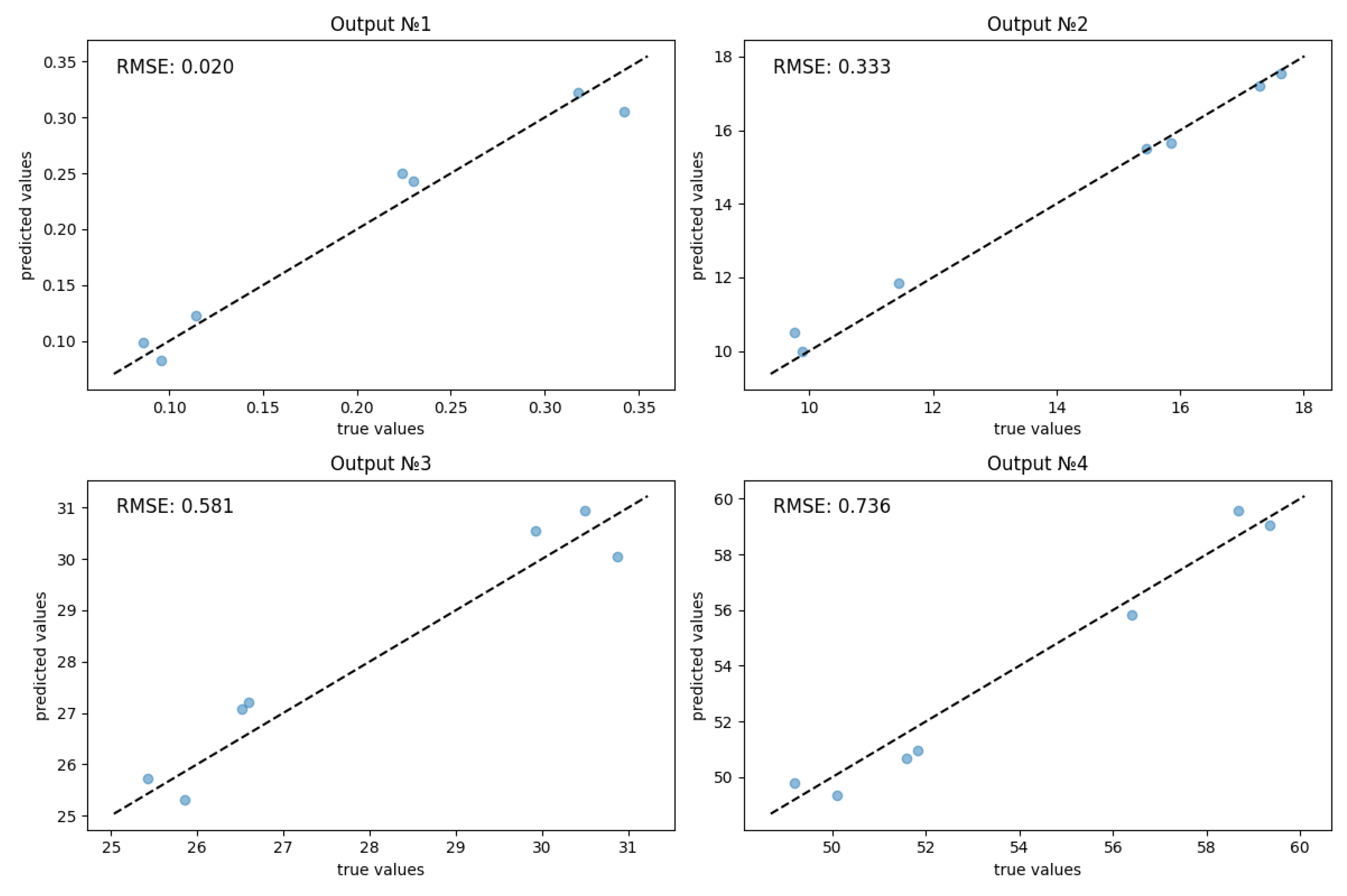
| Decv | 0,020 | 9,49% | 0,960 |
| Lpl | 0,333 | 2,12% | 0,989 |
| ECVCEM | 0,581 | 1,99% | 0,930 |
| ECVAEM | 0,736 | 1,33 | 0,964 |
| Total metrics | 0,417 | 3,74% | 0,961 |
| d1 | Re | Pe | Kel | Decv | Lpl | ECVCEM | ECVAEM | |
|---|---|---|---|---|---|---|---|---|
| Actual Value | 0,05 | 0,05 | 24,39 | 2470000 | 0,334 | 17,54 | 25,3 | 48,7 |
| Predicted | 0,05 | 0,05 | 24,39 | 2470000 | 0,314 | 17,4 | 25,49 | 49,55 |
| Error in % | - | - | - | - | 6 | 0,8 | 0,8 | 1,8 |
| Actual Value | 0,37 | 0,05 | 24,39 | 2470000 | 0,352 | 14,23 | 25,2 | 48,64 |
| Predicted | 0,37 | 0,05 | 24,39 | 2470000 | 0,338 | 13,8 | 25,38 | 49,04 |
| Error in % | - | - | - | - | 4 | 3,1 | 0,8 | 0,8 |
Disclaimer/Publisher’s Note: The statements, opinions and data contained in all publications are solely those of the individual author(s) and contributor(s) and not of MDPI and/or the editor(s). MDPI and/or the editor(s) disclaim responsibility for any injury to people or property resulting from any ideas, methods, instructions or products referred to in the content. |
© 2025 by the authors. Licensee MDPI, Basel, Switzerland. This article is an open access article distributed under the terms and conditions of the Creative Commons Attribution (CC BY) license (http://creativecommons.org/licenses/by/4.0/).


