
Submitted:
02 December 2025
Posted:
03 December 2025
You are already at the latest version
Abstract
Inspired by the well-known experimental connections between X(3872), $Z_{cs}(4220)$, and Y(4620), we systematically study the recently reported strange partner of $T_{cc}$, the $1^{+}$ $cc\bar{q}\bar{s}$ system, and its orbital excitation state $1^{-}$ $cc\bar{q}\bar{s}$. A chiral quark model incorporating SU(3) symmetry is considered to study these two systems. To better investigate their spatial structure, we introduce a precise few-body calculation method, the Gaussian Expansion Method (GEM). In our calculations, we include all possible physical channels, including molecular states and diquark structures, and consider channel coupling effects. To identify the stable structures in the system (bound states and resonance states) we employ a powerful resonance search method, the Real-Scaling Method (RSM). According to our results, in the $1^{+}$ $cc\bar{q}\bar{s}$ system, we obtain two bound states with energies of 3890 MeV and 3940 MeV, as well as two resonance states with energies of 3975 MeV and 4090 MeV. The decay channels of these two resonance states are \( DD_s^* \) and \( D^*D_s \), respectively. In the $1^{-}$ $cc\bar{q}\bar{s}$ system, we obtain only one resonance state, with an energy of 4570 MeV, and two main decay channels: \( DD_{s1}^* \) and \( D^*D_{s1}^{\prime} \). We strongly suggest that experimental groups use our predictions to search for these stable structures.
Keywords:
X(3872)
; Zcs(4220)
; Y(4620)
; Tcc
1. Introduction
The study of multi-quark states has always been one of the best approaches to understanding low-energy quantum chromodynamics (QCD), as multi-quark states can provide more information compared to traditional hadronic structures (mesons and baryons ), especially regarding the color structure within multi-quark configurations. Among these multi-quark structures, the study of tetraquark states has been one of the most important topics in hadron physics. To date, the most frequently observed exotic hadrons experimentally are those with a tetraquark structure, particularly tetraquark states containing charm quarks. Various interpretations of the charm-containing tetraquark states have been discussed, and many other possible charm-containing tetraquark states have also been proposed in the literature.
It is noteworthy that, since the reporting of the [1] in 2003, many experimental groups have successively reported a large number of exotic hadrons with tetraquark structures. However, these tetraquark states are actually correlated in some way. For instance, the , with quantum numbers and quark composition , was initially reported. Subsequently, the [2], with the same quark composition as the but with quantum numbers , and the [3], which shares the same quantum numbers as the but has a different quark composition (), were reported. Recently, the LHCb collaboration reported a new state, the , with quantum numbers and a quark composition of . While considerable theoretical work has been done on this state, its companion states, and , have largely been overlooked in the research.
Currently, theoretical studies on the tetraquark system are relatively scarce, with most of the research focusing on the state, as detailed in the literature [4,5,6,7,8]. For example, in Ref. [4], the authors, based on heavy-quark symmetry and evaluating finite-mass corrections, predicted that the mass of the should be 179 MeV above threshold. However, this result contradicts the findings in Ref. [5], where the authors systematically studied ( and ) tetraquark states with the color-magnetic interaction, taking into account color mixing effects. They found a bound state for the with a binding energy of 84 MeV. In Ref. [6], the authors presented the results of a lattice calculation of states, performed on three dynamical highly improved staggered quark ensembles at lattice spacings of approximately 0.12, 0.09, and 0.06 fm. They ultimately obtained a shallow bound state for the . In Ref. [7], the authors argued that the D-wave component contributes to the formation of a bound state for . After the observation of the , the authors in Ref. [8] utilized the experimental information on the binding energy of to predict a bound state for the .
In this study, we apply the constituent quark model, which incorporates SU(3) symmetry, to systematically explore the system with quantum numbers and . To better describe the dynamics between quarks, we employ the high-precision few-body system calculation method, the Gaussian Expansion Method (GEM). In our analysis, we consider two distinct spatial configurations: meson-meson and diquark-antidiquark, along with all possible color and spin configurations. In principle, a single spatial configuration, along with all possible spatial excitations (S-, P-, D-... waves), is sufficient to describe the wave function of the system. However, considering all possible spatial excitations is computationally challenging. A more efficient approach is to consider the meson-meson and diquark-antidiquark mixing effects, which simplifies the calculations. However, this approach introduces many spurious energy levels. To eliminate these unstable energy levels and accurately identify stable structures (resonant and bound states), we employ the Real-Scaling Method (RSM) [13]in our work.
The structure of this paper is as follows. After the introduction, Sec. II provides a brief description of the quark model, the construction of wave functions, and an overview of the RSM. Our numerical results and related discussions are presented in Sec. III. Finally, a summary is given in Sec. IV.
2. Model Setup
Among the various phenomenological models used to study particle properties, the quark model has always been one of the most successful models, as it has successfully explained and predicted a large number of experimental data. In the quark model[9,10,11,12], its Hamiltonian includes (Eq.1) the mass term , the kinetic term , and the potential term . Since we adopt the chiral quark model, the potential term can be further divided into the confinement potential , the one-gluon exchange potential , and the meson exchange potentials and , as shown in (Eq. 2). These terms correspond to the three fundamental properties of QCD: quark confinement, asymptotic freedom, and chiral symmetry breaking.
Since this paper focuses on the and systems, for the case, the system is in an S-wave, and thus the Hamiltonian only needs to consider central forces. In contrast, for the case, the system includes P-waves, so the Hamiltonian also includes spin-orbit coupling interactions. Therefore, our confinement potential includes both the central force term and the spin-orbit coupling term . Similarly, the one-gluon exchange potential includes and , and the meson exchange potential is divided into , , and . Here, represents pseudoscalar meson exchange, while and correspond to scalar meson exchange. This distinction arises because in the system, and form an SU(3) symmetric pair, and in order to more accurately study the interaction between and , we introduce scalar meson exchange. represents the SU(2) Pauli matrices; represents the SU(3) color and flavor Gell-Mann matrices, respectively; denotes the strong coupling constant of one-gluon exchange. represents the masses of the Goldstone bosons, denotes the corresponding cut-offs, and is the Goldstone-quark coupling constant. The quark tensor operator is given by
Finally, is the standard Yukawa function, defined as
while and are related functions, given by
respectively. After fitting the -family mesons ( as shown in Table 1 ), all the model parameters are determined, which are collected into Table 2.
Now, we turn to the construction of the wave function for the tetraquark structures. The wave function of the system consists of four parts: orbital, spin, flavor, and color. The wave function for each part is constructed in two steps. First, we construct the wave functions for the two clusters separately, and then we couple the two cluster wave functions to form the complete four-body wave function. The first part is the orbital wave function. For the spatial wave function of the system, we consider two possible configurations: the diquark structure and the molecular structure. The primary distinction between their spatial wave functions lies in the arrangement of the constituent quarks. In the molecular structure, the four-quark spatial wave function is encoded as - , while in the diquark structure, it is encoded as - . In this study, for the structure, both the first and second clusters in the spatial part are in S-wave, while in the structure, the second cluster is in P-wave. We then couple this spatial wave function with the relative motion wave function to determine the total orbital wave function. The expressions for the total wave functions are:
The wave function for relative motion, , is constructed using the Gaussian expansion method (GEM). Its functional form is a linear combination of Gaussian basis functions,
Herein, represents the normalization factor, calculated as
The coefficients are the variational parameters determined by the system. The Gaussian exponents are selected to cover a range of scales geometrically, following the relation,
In this study, , , and represent the relative motion wave functions of the first cluster, the second cluster, and the relative motion between the two clusters, respectively. Since we adopt the Real-Scaling Method (RSM)[13], this approach allows us to simultaneously obtain both bound states and resonant states. Specifically, it involves systematically scaling the width of Gaussian functions between the two groups using a scaling factor, denoted by . This is achieved by multiplying all range parameters by , resulting in a transformation of . As increases, the width of the Gaussian functions expands, leading to variations in the system’s intrinsic energy. If a stable structure is present, it remains unaffected by changes in the Gaussian function widths. As shown in Figure 1, when the line representing the resonance state intersects with the line representing the continuum, strong coupling occurs between these two states, and the lines form a non-crossing structure. This structure corresponds to a resonant state in our calculations, and its decay width can be computed using the formula
Since the bound state corresponds to the lowest energy of the system, with no associated decay threshold, it is represented as a horizontal line in our calculations.
Next, we need to construct the flavor wave function. Since we consider two possible structures for the system: the molecular state structure - and the diquark structure -, and since isospin quantum number I is a good quantum number, we fix its third component, , to be . Consequently, for the flavor wave functions, we have two forms:
For the spins of the quark and antiquark, they are indistinguishable, regardless of whether the system is in a diquark or molecular structure. Therefore, the spin wave functions for the sub-clusters are given below
where and represent the third component of quark spin, taking values of and , respectively. By coupling the spin wave functions of the two sub-clusters with Clebsch-Gordan coefficients, the total spin wave function can be written as
In the system studied in this paper, its color structure is crucial, as mentioned in Ref. [5]. QCD requires that multi-quark states must be color-neutral. Therefore, for their molecular state structures, there are two possible configurations: and . For the diquark-antidiquark structure, the two possible configurations are and .
The total wave function of the system is the internal product of color, spin, flavor, and spatial wave functions. The total wave function can be expanded as follows:
where is the antisymmetrization operator. In the system, . Finally, by applying the Rayleigh-Ritz variational principle to the Schrodinger equation, we obtain the eigenvalues and eigenfunctions:
3. Results and Discussions
In this section, we present all the calculation results. We first perform a systematic bound-state calculation for the system with quantum numbers and , including calculations for individual channels as well as the results for complete mixing of all channels. Then, we perform resonance state calculations for these two systems using the Real-Scaling Method (RSM). Finally, we provide the internal structure and width information of the stable states obtained from these calculations.
3.1. Bound-State Calculation
We first discuss the bound-state calculation results for the system, which is the strange partner of . Since its spatial wave function is entirely in S-wave, its total spin is , with three possible combinations: , , and . Considering the molecular state structure, there are two color wave functions: and . Therefore, in the system, we have a total of six molecular state channels: , , , , , and , where we use "" to represent the channel corresponding to the color octet of the molecular state. For the diquark structure, considering the symmetry requirements, the system contains only three diquark channels: 0-1, 1-0, and 1-1. We use the notation "spin" to represent the diquark structure. The single-channel calculation results are listed in rows 2-10 of Table 3. From the results, we observe that the energies of the and channels are quite close, both around 4.0 GeV, while the energies of the other channels are in the range of 4.2-4.3 GeV. The complete coupled-channel calculation shows that we obtain a deep bound state at 3891 MeV, with a binding energy of nearly 70 MeV. This is consistent with the 84 MeV binding energy found in Ref. [6] and aligns qualitatively with the conclusions of Refs. [5,7,8] regarding the existence of a bound state in the system.
Next, we discuss the bound-state calculation results for the system. In order to obtain stable energy, we set the relative motion between the two subclusters as S-wave, while considering the total quantum number , where one of the subclusters is in a P-wave excited state. Combining spin, flavor, and color, we ultimately obtain the following physical channels: , , , , as well as the corresponding color octet states. Due to symmetry constraints, we only consider three diquark structures: 0-1, 1-0, and 1-1. The calculation results are listed in Table 4. We observe that their energies are concentrated between 4.4 GeV and 4.7 GeV, with the energies of the color structures (color octet and diquark structures) being relatively higher, in the range of 4.6-4.7 GeV. In the system, the lowest threshold energy is 4385 MeV, which is significantly lower than the sum of the energies of D and . This is because in the quark model, can interact strongly with via the spin-coupling interactions represented by , , and , leading to a lowering of the energy of the molecular state . Therefore, although the channel coupling interaction lowers the energy of the lowest molecular state to 4386 MeV, it still does not correspond to a bound state.
3.2. Resonance-State Calculation
Next, we discuss the calculation of the resonance states. After considering the channel coupling effects of all possible physical channels, we present the calculation results for the system in Figure 2, and for the system in Figure 3. In the figures, the red lines represent the threshold channels, while the blue lines represent stable structures, including bound states (denoted as B(energy)) and resonance states (denoted as R(energy)).
First, we consider the calculation results for the system. As shown in Figure 2, we obtain a bound state with an energy of 3890 MeV, which is consistent with the lowest energy obtained in the bound-state calculation for the system. Additionally, another state with an energy of 3940 MeV is also observed. This indicates that there are two bound states in the system. Notably, the authors in Ref. [15] also obtained two bound states in a similar double heavy tetraquark system. From our component analysis (Table 5), the former bound state is predominantly composed of , while the latter is a mixture of and , with being the dominant component. I believe the presence of two bound states is due to the fact that the energies of and are relatively close, and there is a strong attraction between them. Furthermore, the system also yields two resonance states, R(3975) and R(4090), both of which are primarily molecular states, with R(4090) having a certain diquark structure component. As a result, the four stable states in the systemB(3890), B(3940), R(3975), and R(4090)all have an internal quark distance (root-mean-square distance) of approximately 1-2 fm, with the molecular component being larger, the distance between quarks is greater. In contrast, for the system, we do not obtain as many stable structures as in the system. We only obtain one resonance state, R(4570), which is predominantly composed of diquark structure, with approximately 30% of the molecular state . Its root-mean-square distance indicates that it is a compact four-quark structure (all within 1 fm).
To facilitate future experimental searches for the resonance states we predict, we performed an analysis of the decay channels of these resonance states, the results of which are presented in Figure 4. R(3975) has only one decay channel, (decay width 0.8 MeV), and does not require additional analysis. R(4090) has two decay channels: and , with the latter dominating (approximately 98%). R(4570) has three decay channels: , , and , with the latter two being the main decay channels, accounting for 47% and 41%, respectively.

Table 6.
Various decay channels and corresponding decay widths of the obtained resonances. (unit: MeV)
Table 6.
Various decay channels and corresponding decay widths of the obtained resonances. (unit: MeV)
| Decay channels | ||||||
|---|---|---|---|---|---|---|
| 0.8 | 1.1 | - | ||||
| - | 46.8 | - | ||||
| - | - | 17.1 | ||||
| - | - | 65.0 | ||||
| - | - | 56.5 | ||||
| Total | 0.8 | 47.9 | 138.6 |
4. Summary
In the framework of the chiral quark model, we performed bound-state and resonance-state calculations for the system.
Based on our bound-state calculation results, in the system, although no individual channel is a bound state, after complete channel coupling, we obtained a deep bound state with a binding energy of 3965 MeV, which is consistent with most theoretical studies. In the system, we did not obtain a bound state.
The resonance-state calculations yielded significant results. In the system, we found two bound states, B(3890) and B(3940), with the primary components being and , respectively, as well as two resonance states, R(3975) and R(4090), with the primary components being and , respectively. Notably, R(4090) contains a significant diquark component. Therefore, B(3890), B(3940), and R(3975) exhibit a clear molecular structure with root-mean-square distances of 1-2 fm. The system contains only one resonance state, R(4575), which is primarily composed of a diquark structure, and thus its quark distance is within 1 fm.
In conclusion, we identified five stable structures in the system: two bound states, B(3890) and B(3940), and three resonance states, R(3975), R(4090), and R(4575). Their main decay channels are , , and , , respectively. We strongly suggest that experimental groups search for these structures, especially in the system.
Acknowledgments
This work is supported partly by the National Science Foundation of China under Contract No. 12205249. Y. T. is supported by the Funding for School-Level Research Projects of Yancheng Institute of Technology under Grant No. xjr2022039 and 2025010.
References
- S. K. Choi et al. [Belle], Phys. Rev. Lett. 91, 262001 (2003). [CrossRef]
- S. Jia et al. [Belle], Phys. Rev. D 101, no.9, 091101 (2020). [CrossRef]
- M. Ablikim et al. [BESIII], Phys. Rev. Lett. 126, no.10, 102001 (2021). [CrossRef]
- E. J. Eichten and C. Quigg, Phys. Rev. Lett. 119, no.20, 202002 (2017). [CrossRef]
- S. Q. Luo, K. Chen, X. Liu, Y. R. Liu and S. L. Zhu, Eur. Phys. J. C 77, no.10, 709 (2017). [CrossRef]
- P. Junnarkar, N. Mathur and M. Padmanath, Phys. Rev. D 99, no.3, 034507 (2019). [CrossRef]
- C. Deng and S. L. Zhu, Phys. Rev. D 105, no.5, 054015 (2022). [CrossRef]
- M. Karliner and J. L. Rosner, Phys. Rev. D 105, no.3, 034020 (2022). [CrossRef]
- Y. Tan, Z. X. Ma, X. Chen, X. Hu, Y. Yang, Q. Huang and J. Ping, Phys. Rev. D 111, no.9, 096018 (2025). [CrossRef]
- Y. Tan, X. Liu, X. Chen, Y. Yang, H. Huang and J. Ping, Phys. Rev. D 110, no.1, 016005 (2024). [CrossRef]
- Y. Tan, X. Liu, X. Chen, Y. Wu, H. Huang and J. Ping, Phys. Rev. D 109, no.7, 076026 (2024). [CrossRef]
- Y. Tan, Y. Wu, H. Huang and J. Ping, Universe 10, no.1, 17 (2024). [CrossRef]
- J. Simons, J. Chem. Phys. 75, no.5, 2465 (1981). [CrossRef]
- Navas et al. [Particle Data Group], Phys. Rev. D 110, no.3, 030001 (2024). [CrossRef]
- G. Yang, J. Ping and J. Segovia, Phys. Rev. D 101, no.1, 014001 (2020). [CrossRef]
Figure 1.
Two types of resonance states: (a) resonance with weak coupling (or no coupling) to the scattering states; (b) resonance with strong coupling to the scattering states.
Figure 1.
Two types of resonance states: (a) resonance with weak coupling (or no coupling) to the scattering states; (b) resonance with strong coupling to the scattering states.
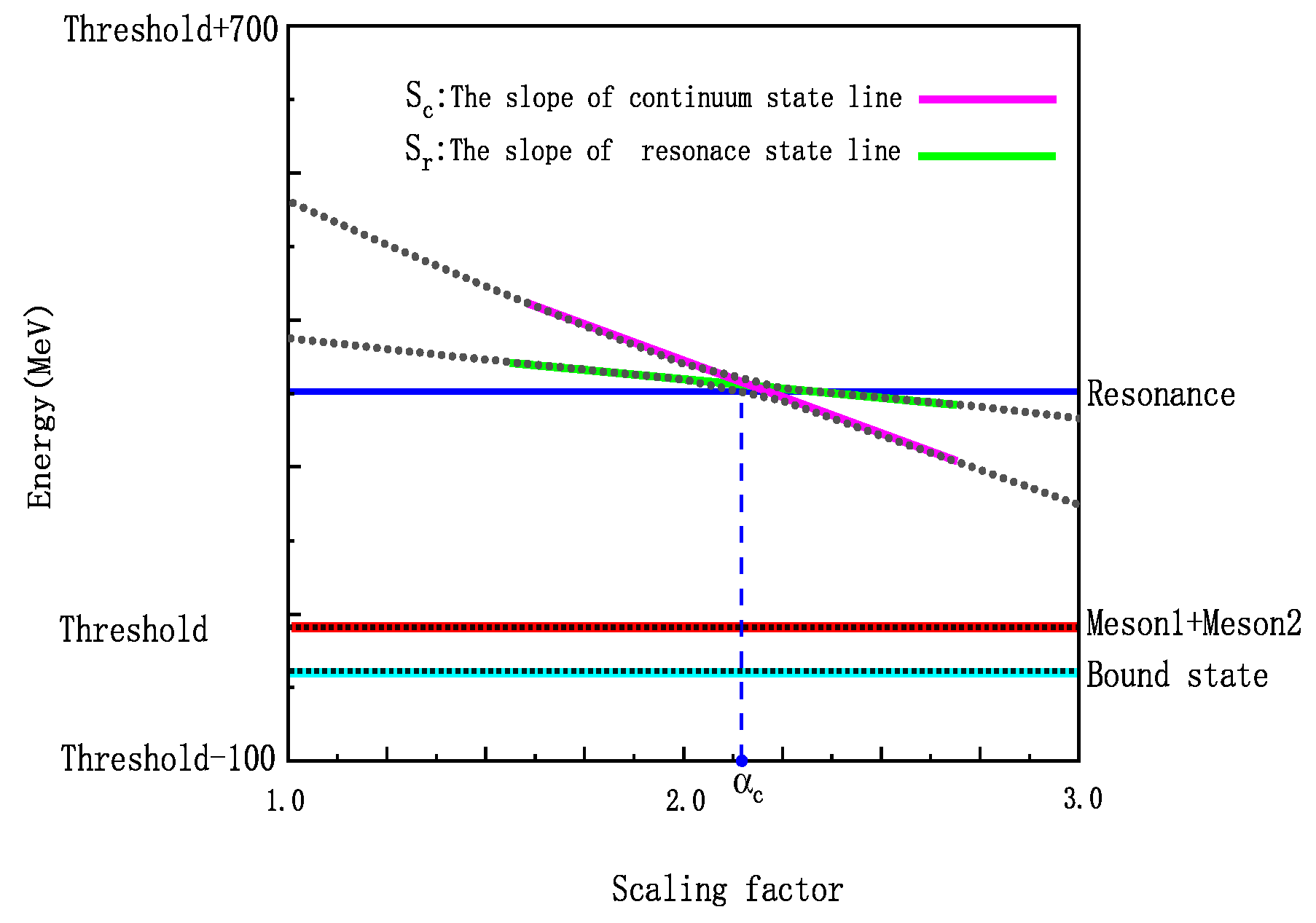
Figure 2.
Real-scaling results for the with system.
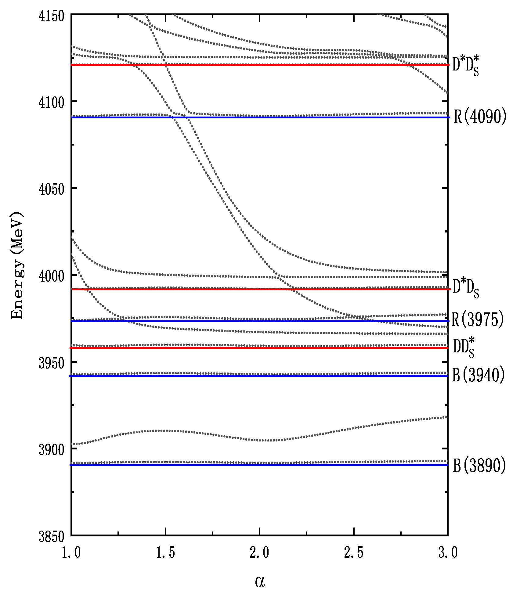
Figure 3.
Real-scaling results for the with system.
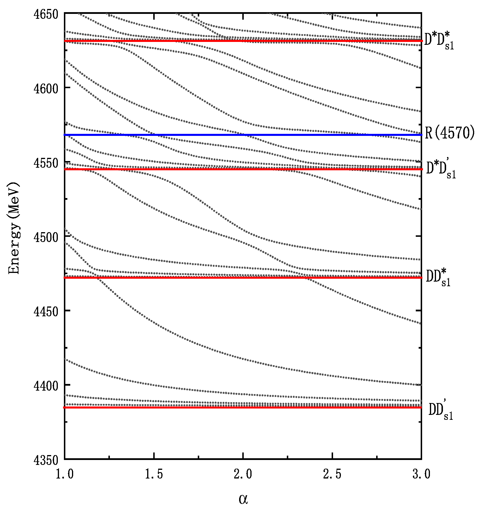
Figure 4.
Decay of Resonances R(4090) and R(4570) to Various Threshold Channels
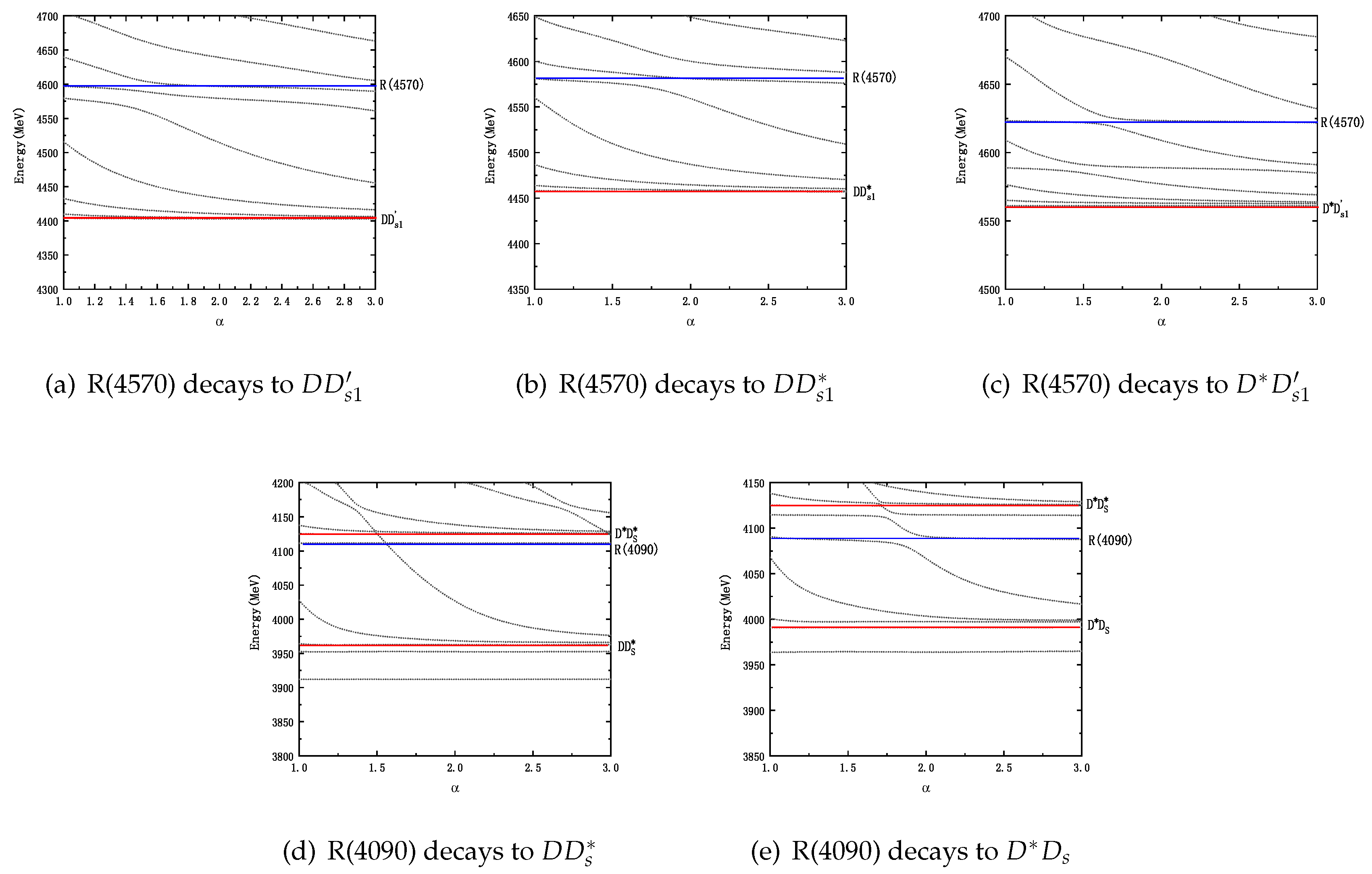
Table 1.
Results of the spectrum calculation.
| D | ||||||
|---|---|---|---|---|---|---|
| This work | 1861 | 2021 | 1977 | 2104 | 2541 | 2595 |
| EXP. (PDG)[14] | 1864 | 2010 | 1968 | 2107 | 2460 | 2535 |
Table 2.
Quark model parameters (, , , ).
| Quark masses | (MeV) | 490 |
|---|---|---|
| (MeV) | 1650 | |
| Goldstone bosons | 3.5 | |
| 2.2 | ||
| 7.0 | ||
| 2.5 | ||
| 1.2 | ||
| 0.54 | ||
| -15 | ||
| Confinement | (MeV·fm−2) | 98 |
| (MeV) | -18.1 | |
| OGE | 1.15 | |
| 0.85 | ||
| 0.74 | ||
| 0.56 | ||
| (MeV) | 80.9 |
Table 3.
Results of the bound state calculations for the with system. The indices i, j, k, and l represent the orbital, spin, flavor, and color quantum numbers, respectively (unit: MeV).
Table 3.
Results of the bound state calculations for the with system. The indices i, j, k, and l represent the orbital, spin, flavor, and color quantum numbers, respectively (unit: MeV).
| Channel | E | Percent | |
|---|---|---|---|
| 3967 | |||
| 4343 | |||
| 3999 | |||
| 4342 | |||
| 4126 | |||
| 4312 | |||
| 0-1 | 4346 | ||
| 1-0 | 4336 | ||
| 1-1 | 4247 | ||
| complete coupled-channels: | 3891 | ||
| Threshold(D+): | 3965 | ||
Table 4.
Results of the bound state calculations for the with system. The indices i, j, k, and l represent the orbital, spin, flavor, and color quantum numbers, respectively (unit: MeV).
Table 4.
Results of the bound state calculations for the with system. The indices i, j, k, and l represent the orbital, spin, flavor, and color quantum numbers, respectively (unit: MeV).
| Channel | E | Percent | |
|---|---|---|---|
| 4404 | |||
| 4711 | |||
| 4458 | |||
| 4737 | |||
| 4563 | |||
| 4685 | |||
| 4617 | |||
| 4688 | |||
| 0-1 | 4689 | ||
| 1-0 | 4742 | ||
| 1-1 | 4563 | ||
| complete coupled-channels: | 4386 | ||
| Threshold(D+): | 4385 | ||
Table 5.
Main Component Information of Bound States and Resonant States, and the Root-Mean-Square Distance of Internal Quarks (in fm). "c.s." denotes colorful structure, including color octet and diquark structures.
Table 5.
Main Component Information of Bound States and Resonant States, and the Root-Mean-Square Distance of Internal Quarks (in fm). "c.s." denotes colorful structure, including color octet and diquark structures.
| Main Components | |||||
|---|---|---|---|---|---|
| B(3890) | + others | 1.3 | 0.4 | 1.4 | 0.6 |
| B(3940) | + + others | 2.0 | 0.4 | 2.1 | 0.6 |
| R(3975) | + others | 2.2 | 0.5 | 2.5 | 0.5 |
| R(4090) | ++ others | 1.1 | 0.5 | 1.2 | 0.6 |
| R(4575) | ++ others | 0.8 | 0.8 | 1.0 | 0.9 |
Disclaimer/Publisher’s Note: The statements, opinions and data contained in all publications are solely those of the individual author(s) and contributor(s) and not of MDPI and/or the editor(s). MDPI and/or the editor(s) disclaim responsibility for any injury to people or property resulting from any ideas, methods, instructions or products referred to in the content. |
© 2025 by the authors. Licensee MDPI, Basel, Switzerland. This article is an open access article distributed under the terms and conditions of the Creative Commons Attribution (CC BY) license (http://creativecommons.org/licenses/by/4.0/).
Copyright: This open access article is published under a Creative Commons CC BY 4.0 license, which permit the free download, distribution, and reuse, provided that the author and preprint are cited in any reuse.


