Submitted:
02 December 2025
Posted:
04 December 2025
You are already at the latest version
Abstract
This paper presents a complete, constructive derivation of the Steane [[7,1,3]] quantum error-correcting code using a unified framework that bridges GF(4) algebra, binary symplectic representation, and stabilizer formalism. We demonstrate how classical coding theory, finite-field arithmetic, and symplectic geometry naturally converge to form a comprehensive foundation for quantum error correction. Starting from the classical Hamming [7,4,3] code, we provide explicit constructions showing: (1) how GF(4) encodes the Pauli group modulo phases, (2) how the symplectic inner product on F2n2 captures commutativity, (3) how syndrome extraction reduces to binary matrix multiplication, and (4) how transversal Clifford gates emerge from symplectic transformations. The step-by-step derivation encompasses stabilizer construction, centralizer analysis, logical operator identification, code distance verification, and fault-tolerant syndrome measurement via flagged circuits. All results are derived using elementary finite-field and binary linear algebra, ensuring the exposition is self-contained and accessible. We further illustrate how this algebraic framework extends naturally to modern quantum LDPC codes. This work serves as both a pedagogical tutorial for students entering quantum error correction and a unified reference for researchers implementing stabilizer codes in practice
Keywords:
quantum error correction
; stabilizer codes
; GF(4)
; symplectic representation
; Steane code
; CSS codes
; fault tolerance
; pedagogical tutorial
1. Introduction: The Need for Unified Understanding
Quantum error correction (QEC) constitutes the mathematical backbone of fault-tolerant quantum computation. While the stabilizer formalism [1] provides a comprehensive framework, its pedagogical presentation often fragments into isolated components: group theory for Pauli algebras, finite-field arithmetic for code construction, symplectic geometry for commutativity analysis, classical coding theory for distance bounds, and circuit design for fault-tolerant implementation. This fragmentation obscures the elegant algebraic unity that makes stabilizer codes both theoretically profound and practically implementable.
The recent surge in quantum low-density parity-check (QLDPC) codes [4,5] and advanced fault-tolerant protocols [6] relies fundamentally on GF(4) representations and binary symplectic methods. Yet a coherent, constructive derivation connecting these elements from first principles remains conspicuously absent from the literature. Students and researchers must synthesize understanding from disparate sources, each employing distinct notation and assumptions—a significant barrier to entry.
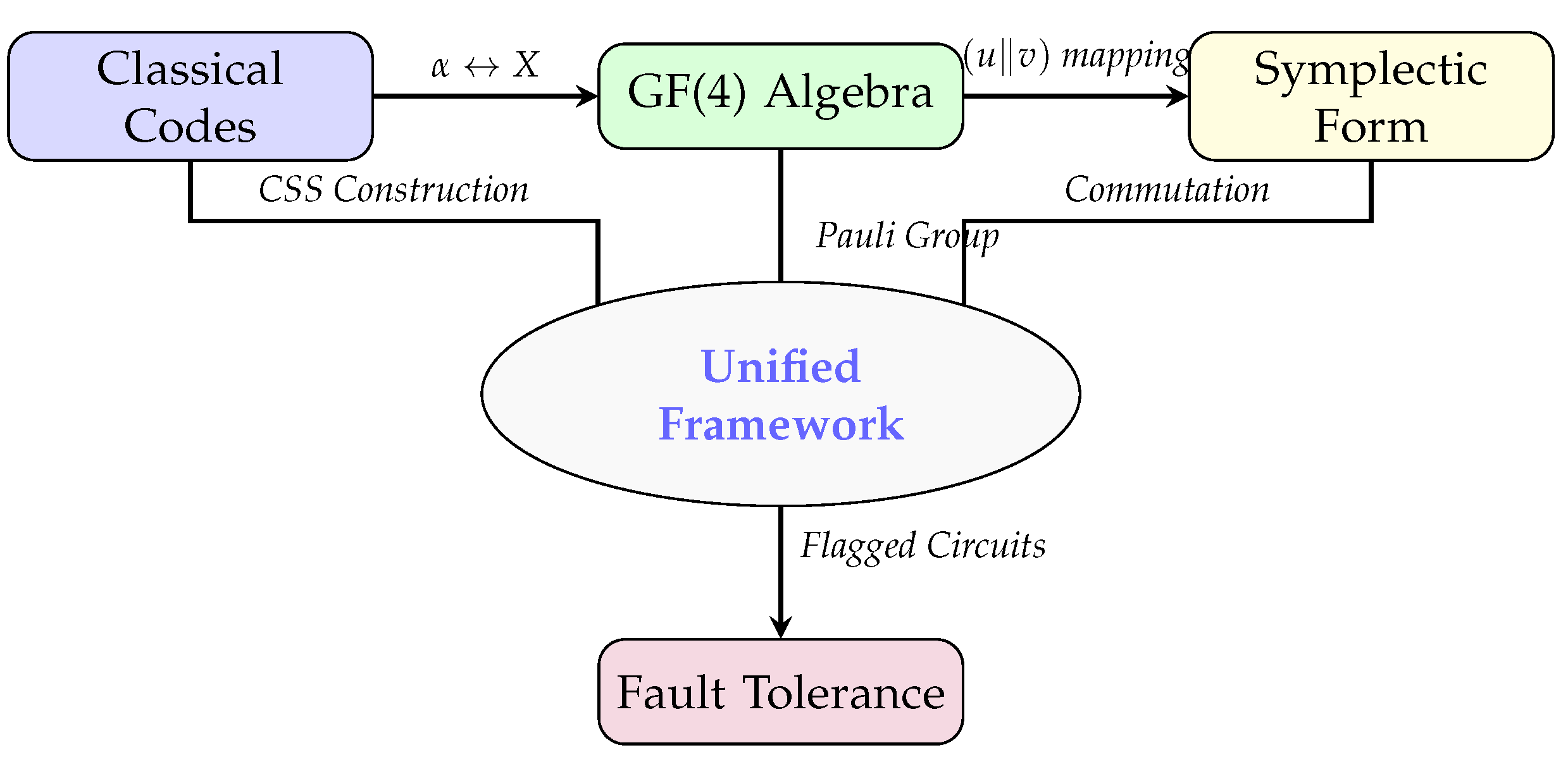
Figure 1.
Unified framework connecting classical coding theory, GF(4) algebra, symplectic geometry, stabilizer formalism, and fault-tolerant implementation.
Figure 1.
Unified framework connecting classical coding theory, GF(4) algebra, symplectic geometry, stabilizer formalism, and fault-tolerant implementation.
Contributions and Organization
This paper presents a unified framework that systematically connects all essential components of stabilizer quantum error correction. Our specific contributions include:
- Establishing an explicit, constructive isomorphism between GF(4) and the Pauli group modulo phases, providing an algebraic foundation for quantum codes
- Demonstrating how binary symplectic representation transforms quantum commutation into matrix multiplication via the symplectic inner product
- Providing a step-by-step construction of the Steane [[7,1,3]] code from the classical Hamming code, illustrating the CSS construction in complete detail
- Deriving all code properties—stabilizers, logical operators, distance, syndromes—using only linear algebra over finite fields
- Showing how transversal Clifford gates emerge naturally from the symplectic structure
- Presenting explicit fault-tolerant measurement circuits directly derived from the algebraic framework
- Illustrating how this foundation extends systematically to subsystem and QLDPC codes
Our approach is intentionally constructive and pedagogical: every claim is justified by explicit calculation using only finite-field arithmetic and binary linear algebra. By presenting this unified framework, we aim to lower the barrier to entry for new researchers while providing experienced practitioners with a coherent mathematical foundation for code design and analysis.
The paper is organized as follows: Section 2 introduces GF(4) algebra and its correspondence with Pauli operators. Section 3 develops the binary symplectic representation. Section 4 reviews the classical Hamming code foundation. Section 5-9 construct the Steane code and analyze its properties. Section 10-11 discuss transversal gates and fault-tolerant measurement. Section 12-13 extend the framework to modern codes. Section 14 provides concluding remarks.
2. GF(4) Algebra: The Algebraic Language of Pauli Operators
2.1. Finite Field GF(4) Structure
The finite field GF(4) serves as the natural algebraic structure for representing Pauli operators modulo phases. Defined as:
with addition and multiplication modulo the irreducible polynomial , satisfying:

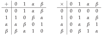
Table 1.
Arithmetic tables for GF(4). These capture the multiplication rules of Pauli matrices when ignoring global phases.
Table 1.
Arithmetic tables for GF(4). These capture the multiplication rules of Pauli matrices when ignoring global phases.
| + | 0 | 1 | × | 0 | 1 | ||||
|---|---|---|---|---|---|---|---|---|---|
| 0 | 0 | 1 | 0 | 0 | 0 | 0 | 0 | ||
| 1 | 1 | 0 | 1 | 0 | 1 | ||||
| 0 | 1 | 0 | 1 | ||||||
| 1 | 0 | 0 | 1 |
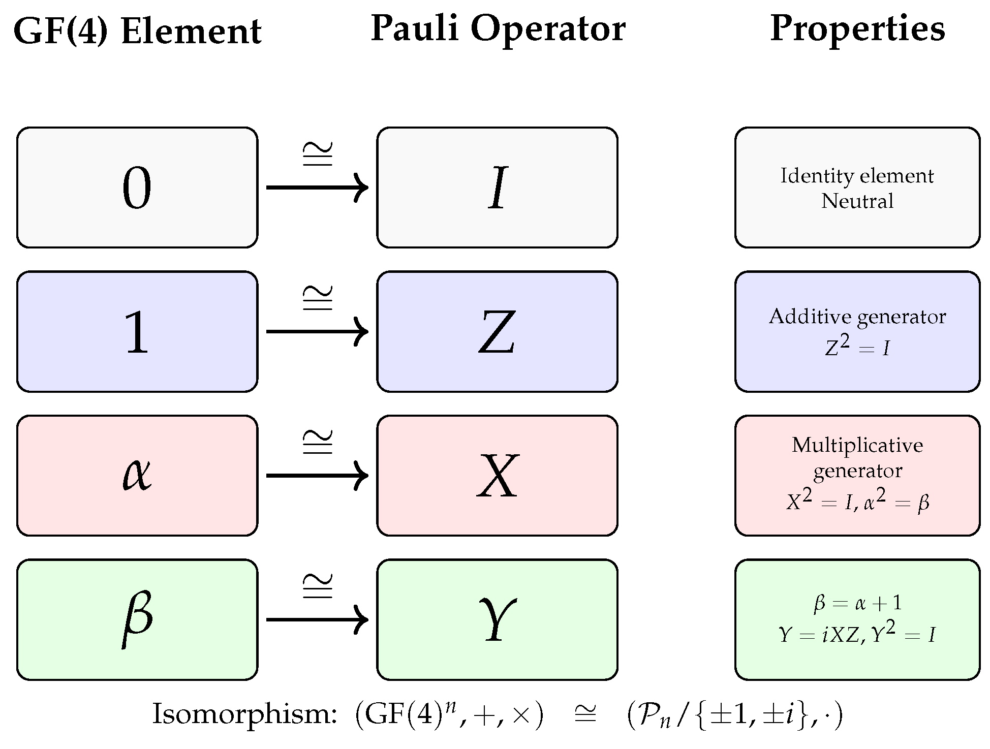
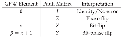
Conceptual Insight: The structure of GF(4) naturally encodes the multiplication rules of Pauli matrices when we ignore global phases. Specifically, corresponds to X, 1 corresponds to Z, and corresponds to .
2.2. GF(4)–Pauli Correspondence
The isomorphism between GF(4) and single-qubit Pauli operators modulo phases is:
This correspondence preserves the group structure up to global phases. For example:
For n qubits, the vector space encodes all Pauli operators (modulo phases), where each component specifies the Pauli acting on the corresponding qubit.
Figure 2.
Structural isomorphism between GF(4) algebra and Pauli operators modulo phases. The correspondence preserves group structure: addition in GF(4) corresponds to operator multiplication up to phases.
Figure 2.
Structural isomorphism between GF(4) algebra and Pauli operators modulo phases. The correspondence preserves group structure: addition in GF(4) corresponds to operator multiplication up to phases.
Example: Logical Operator Representation
The logical operator for the Steane code is . In GF(4) representation:
This compact representation enables algebraic manipulation of logical operators using finite-field arithmetic while maintaining the quantum mechanical structure.
3. Binary Symplectic Representation: From Abstract Algebra to Practical Computation
3.1. Binary Encoding for Efficient Implementation
While GF(4) provides elegant algebraic representation, binary encoding enables practical computation and hardware implementation. Any Pauli operator P on n qubits can be encoded as a binary vector , where:
- if P has an X or Y on qubit j
- if P has a Z or Y on qubit j
This encoding yields the explicit single-qubit mapping:
Table 2.
Binary symplectic representation of single-qubit Pauli operators.
| Pauli Operator | Symbol | Binary Encoding |
|---|---|---|
| Identity | I | |
| Bit flip | X | |
| Phase flip | Z | |
| Combined flip | Y |
For multi-qubit operators, the representation concatenates these single-qubit representations. For example, corresponds to .
3.2. Symplectic Inner Product: Quantum Commutation as Matrix Multiplication
The symplectic inner product on is defined as:
where · denotes the usual dot product in .
Theorem 1
(Commutation Criterion). Two Pauli operators P and Q commute if and only if their binary symplectic representations satisfy .
Proof.
The commutator equals where . The proof follows directly from the anti-commutation relations and the linearity of the symplectic product. □
Conceptual Significance: This theorem transforms quantum mechanical commutation—a physical property—into a simple binary matrix calculation. This transformation is essential for efficient stabilizer code analysis, simulation, and implementation.
3.3. Bridging GF(4) and Binary Representations
Conversion between representations is algorithmically straightforward:
|
Algorithm 1: Conversion between GF(4) and binary symplectic representations
|
|
4. Classical Foundation: Hamming [7,4,3] Code
Quantum CSS codes are constructed from pairs of classical linear codes. The Steane [[7,1,3]] code originates from the classical Hamming [7,4,3] code, a perfect single-error-correcting code with remarkable algebraic properties.
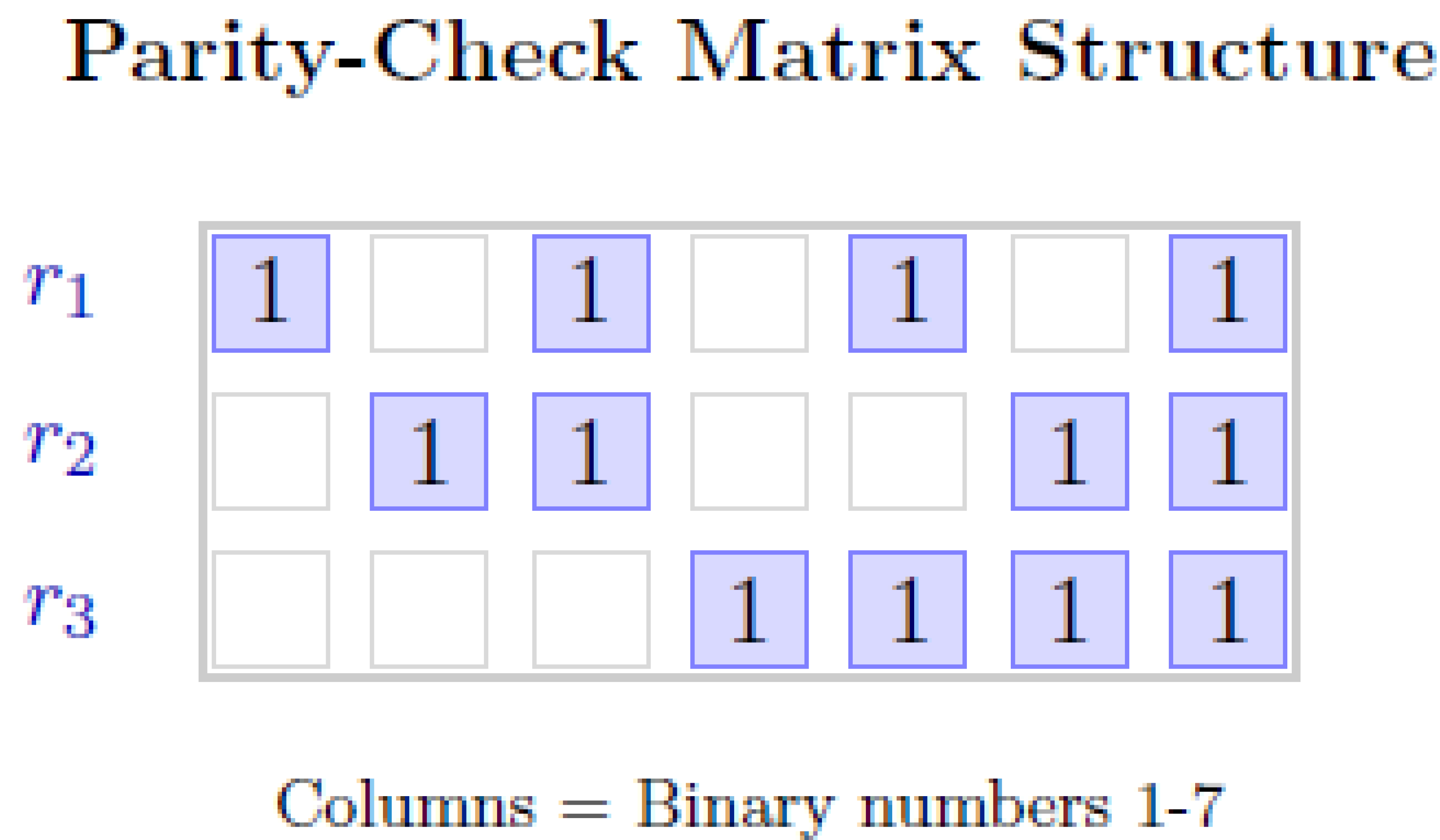
4.1. Matrix Structure and Column Construction
The Hamming code is defined by its parity-check matrix:
Key structural insight: The columns of H are all non-zero binary vectors of length 3, arranged in lexicographic order. Specifically, column i represents the binary encoding of the number i:
Figure 3.
Structure of Hamming code parity-check matrix H. Each column is a distinct binary number, providing unique error signatures.
Figure 3.
Structure of Hamming code parity-check matrix H. Each column is a distinct binary number, providing unique error signatures.
4.2. Code Parameters and Generator Matrix
The Hamming code has parameters , where:
- : code length (number of bits)
- : dimension (information bits), since
- : minimum distance (smallest weight of non-zero codewords)
The generator matrix in systematic form is:
The code space is , containing codewords.
4.3. Syndrome Decoding Mechanism
The Hamming code’s decoding is exceptionally simple due to its column structure. For any single-bit error vector (with 1 at position i and 0 elsewhere):
This means the syndrome is the column where the error occurred. Decoding reduces to a simple table lookup.
Figure 4.
Horizontal layout of syndrome decoding process.

4.4. Syndrome Lookup Table
The complete decoding table for all single-bit errors is remarkably simple:
Table 3.
Syndrome lookup table for Hamming [7,4,3] code.
| Syndrome s | Binary Value | Error Position |
|---|---|---|
| 000 | 0 | No error |
| 100 | 1 | Position 1 |
| 010 | 2 | Position 2 |
| 110 | 3 | Position 3 |
| 001 | 4 | Position 4 |
| 101 | 5 | Position 5 |
| 011 | 6 | Position 6 |
| 111 | 7 | Position 7 |
4.5. Distance Analysis and Error Detection Capabilities
The distance follows directly from the column properties:
- Single-error detection: All columns are non-zero, so for any single error.
- Double-error detection: All columns are distinct, so for any two errors.
- Distance guarantee: No three columns sum to zero, so the smallest undetectable error has weight 3.
The weight enumerator confirms the distance:
showing no codewords of weight 1 or 2.
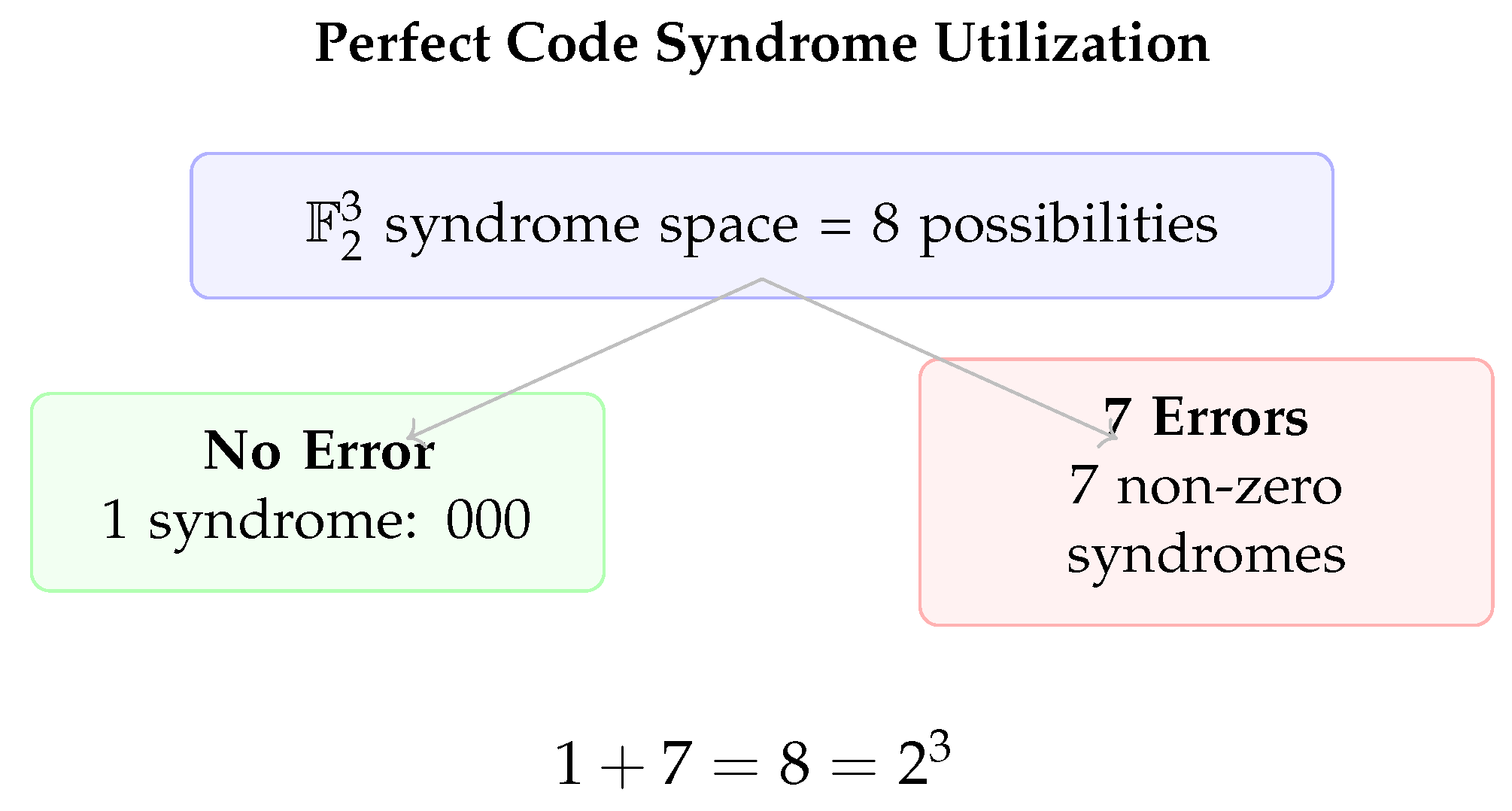
4.6. Perfect Code Property
The Hamming code is a perfect single-error-correcting code, meaning it saturates the Hamming bound:
where . For :
Interpretation: All possible syndromes are utilized exactly:
- 1 syndrome for no error (000)
- 7 syndromes for the 7 possible single-bit errors
- No wasted syndrome space
Figure 5.
Perfect Hamming code uses all syndrome possibilities.
4.7. Importance for Quantum Error Correction
The Hamming code’s properties make it ideal as a foundation for quantum CSS codes:
Table 4.
Transfer of classical properties to quantum error correction.
| Classical Property | Quantum Significance |
|---|---|
| Unique syndromes | Enables unambiguous identification of single-qubit Pauli errors (X, Y, Z) |
| Distance | Directly transfers to quantum distance, enabling correction of arbitrary single-qubit errors |
| Orthogonality | Ensures automatic commutation between X and Z stabilizers in CSS construction |
| Perfect code efficiency | Optimal use of syndrome space translates to efficient quantum error correction |
| Systematic generator matrix | Facilitates construction of logical operators and fault-tolerant circuits |
| Symmetric structure | Allows identical treatment of X and Z errors, simplifying implementation |
4.8. From Classical to Quantum: CSS Construction
The Steane [[7,1,3]] code is constructed using the CSS (Calderbank-Shor-Steane) framework with the Hamming code :
- Use the same code C for both X-type and Z-type stabilizers
- The orthogonality condition ensures X and Z stabilizers commute
-
Quantum parameters follow from the CSS formula:where:
- -
- : Physical qubits (same as classical bits)
- -
- : Logical qubits encoded
- -
- : Quantum distance (inherited from classical)
4.9. Summary: Why Hamming is the Ideal Foundation
The Hamming [7,4,3] code is uniquely suited as a foundation for quantum error correction because:
- Optimal parameters: As the smallest non-trivial perfect code, it provides the minimal overhead for single-error correction.
- Algebraic simplicity: The column structure makes decoding trivial—syndrome directly equals error location.
- Self-orthogonality: ensures the CSS construction automatically yields commuting stabilizers.
- Symmetry: Identical treatment of all bit positions enables straightforward generalization to quantum errors.
- Practicality: With only 7 physical bits/qubits, it remains implementable while providing meaningful error protection.
- Pedagogical value: Its simplicity makes it an ideal teaching example while containing all essential features of more complex codes.
This classical foundation provides the mathematical bedrock upon which the quantum Steane [[7,1,3]] code is built, inheriting the Hamming code’s elegance while adding quantum error correction capabilities.
5. Constructive Derivation of the Steane [[7,1,3]] Code
5.1. CSS Construction: Bridging Classical and Quantum Codes
The Calderbank-Shor-Steane (CSS) construction [2] builds quantum codes from pairs of classical codes. Given a classical linear code C with parity-check matrix H, the CSS code uses:
- X-stabilizers: Generators with supports given by rows of H, acting as X operators
- Z-stabilizers: Generators with identical supports, acting as Z operators
For the Steane code, we use the same Hamming code for both X and Z stabilizers. This symmetric construction guarantees automatic commutation between X and Z stabilizers due to the orthogonality condition over .
5.2. Explicit Stabilizer Generators
5.2.1. Z-Type Stabilizers
From the rows of H:
In binary symplectic form:
5.2.2. X-Type Stabilizers
Identical supports but with X operators:
In binary symplectic form:
5.3. Verification of Commutation Relations
All stabilizers pairwise commute. Let’s verify one non-trivial case explicitly:
Example: Check commutation between and :
All other pairs commute similarly because over , ensuring the symplectic inner product vanishes for all cross terms.
6. Symplectic Stabilizer Matrix
The full stabilizer group is generated by the six operators above. The symplectic stabilizer matrix compactly represents all generators:
The rank of M is 6 (full rank), as the rows are linearly independent. This matrix representation enables efficient computation of syndromes and analysis of code properties.
7. Logical Operators and Centralizer Structure
7.1. Centralizer Dimension and Logical Qubits
The centralizer consists of all Pauli operators that commute with every stabilizer. In symplectic terms, is the kernel of the map defined by the symplectic product with rows of M.
The dimension follows from fundamental linear algebra:
Table 5.
Dimensional analysis of the Steane code’s operator space.
| Space | Dimension | Interpretation |
|---|---|---|
| Full Pauli space (mod phases) | All operators on 7 qubits | |
| Stabilizer group S | 6 independent generators | |
| Centralizer | 8 | Operators commuting with S |
| Logical operators | 2 | Encodes 1 logical qubit |
7.2. Canonical Logical Operators
Standard choices for logical operators that respect the code’s symmetry are:
In binary symplectic form:
7.3. Explicit Verification of Logical Properties
-
Commutation with stabilizers: For any X-stabilizer :Similarly for Z-stabilizers and .
- Anti-commutation between logicals:
- Not in stabilizer group: Both have weight 7, while all stabilizers have weight 4 and specific patterns not matching all-ones.
8. Syndrome Extraction and Decoding
8.1. Syndrome Calculation: From Quantum Physics to Linear Algebra
Let be a Pauli error. Its syndrome is computed as:
Physical Interpretation: The syndrome has two 3-bit components:
Specifically:
8.2. Single-Qubit Error Syndrome Table
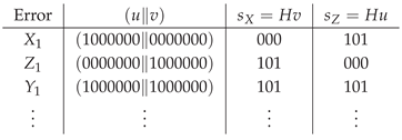
Table 6.
Complete syndrome table for single-qubit Pauli errors on the Steane code. Each of the 21 possible errors produces a unique syndrome.
Table 6.
Complete syndrome table for single-qubit Pauli errors on the Steane code. Each of the 21 possible errors produces a unique syndrome.
| Qubit | Error Type | Syndrome | |
|---|---|---|---|
| 1 | |||
| 2 | |||
| 3 | |||
| ⋮ (Qubits 4-7 follow similar pattern with unique syndromes) | |||
8.3. Worked Example: X Error on Qubit 3
Consider error . Then:
Syndrome calculation:
Thus , meaning:
- X-stabilizers: all measure ()
- Z-stabilizers: and measure , measures ()
This syndrome uniquely identifies an X error on qubit 3, enabling precise error correction.
9. Code Distance Calculation
9.1. Methodology for Distance Determination
The code distance d is the minimum weight of a non-trivial logical operator (an operator in ). We verify through systematic analysis.
9.2. Weight-1 and Weight-2 Errors
- Weight-1: All detectable. For any single-qubit Pauli E, either or because all columns of H are non-zero.
- Weight-2: Consider any weight-2 Pauli . The syndrome is the XOR of columns i and j of H (for X or Y errors). Since no two columns of H are identical, no two columns sum to zero, so all weight-2 errors are detected.
9.3. Weight-3 Undetectable Error
To find a weight-3 undetectable error, we need such that , where has ones at positions . This means must correspond to three columns of H that sum to zero.
The Hamming code’s generator matrix is:
The first row gives codeword with weight 3. This corresponds to . Verify:
Thus has zero syndrome and weight 3. It commutes with all stabilizers but is not in the stabilizer group (all X-stabilizers have weight 4 with different patterns). Therefore .
Since weight-1 and weight-2 errors are all detected, we conclude .
10. Transversal Clifford Gates
10.1. Hadamard Gate: Symmetry Between X and Z
The Hadamard gate H exchanges on a single qubit. On n qubits, transforms the symplectic representation as:
For the Steane code:
- X-stabilizers = Z-stabilizers
- Z-stabilizers = X-stabilizers
- Logical
- Logical
Thus implements logical Hadamard transversally.
10.2. Phase Gate: Implementation up to Global Phase
The phase gate transforms:
Applied transversally to the Steane code:
Since global phases are ignored in the Pauli group modulo phases, implements logical phase up to a global phase.
10.3. CNOT Gate: Transversal Entanglement
For CNOT with control c and target t, the symplectic transformation is:
Applied transversally (qubit i of control block to qubit i of target block), this transformation preserves the stabilizer group of two Steane code blocks, implementing logical CNOT.
11. Fault-Tolerant Stabilizer Measurement
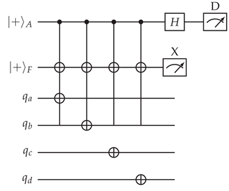
11.1. The Need for Flagged Circuits
Direct measurement of stabilizers using a single ancilla qubit can propagate a single fault to multiple data qubits, creating weight-2 data errors that may be uncorrectable. Flagged circuits [6] prevent this by using an additional flag qubit to detect potentially dangerous fault configurations.
11.2. Flagged Measurement Circuit Design
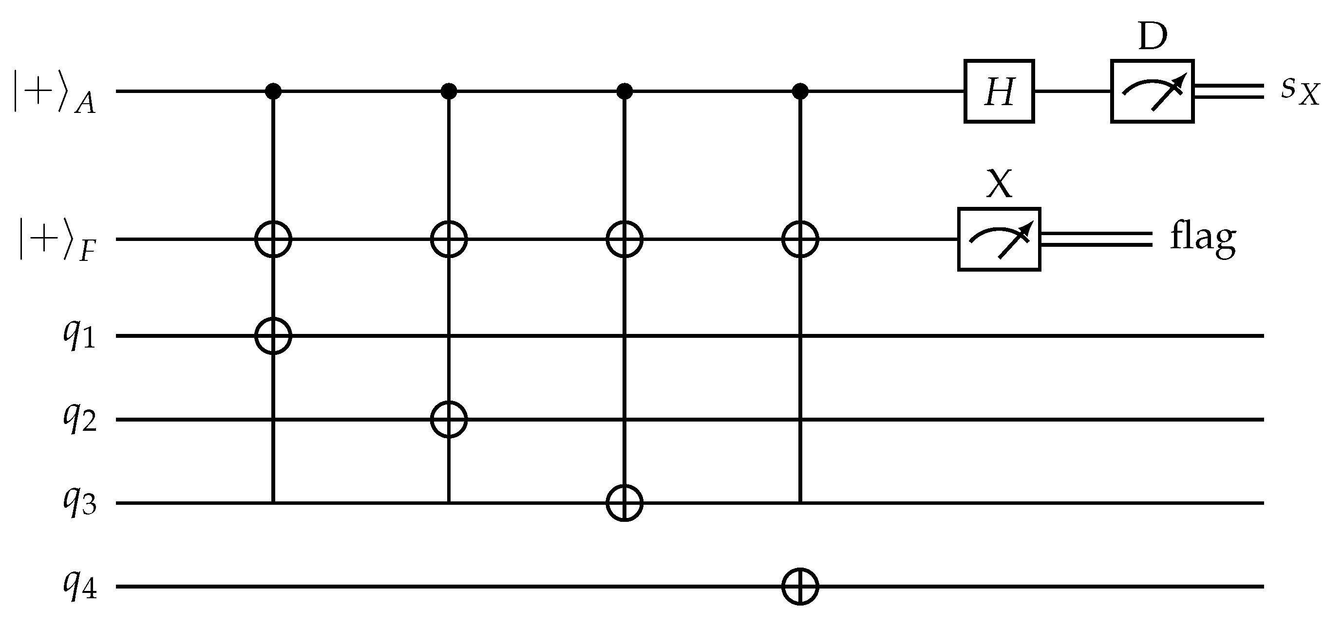
Figure 6.
Flagged circuit for measuring stabilizer. The circuit measures the syndrome on ancilla A while using flag qubit F to detect hook errors. For Z-stabilizers, replace + with 0 and reverse CNOT directions.
Figure 6.
Flagged circuit for measuring stabilizer. The circuit measures the syndrome on ancilla A while using flag qubit F to detect hook errors. For Z-stabilizers, replace + with 0 and reverse CNOT directions.
11.3. Error Propagation Analysis
A single fault can occur at any location:
- Ancilla preparation error: Propagates to at most one data qubit via CNOT back-action.
- Gate error: CNOT error propagates to either data or flag, not both.
- Measurement error: Detected by repetition or post-selection.
The flag measurement outcome indicates whether a potentially harmful fault occurred, enabling adaptive correction or rejection of that syndrome measurement round.
12. Noise Model and Pseudo-Threshold
12.1. Realistic Circuit-Level Noise
Consider a comprehensive noise model:
- Single-qubit depolarizing noise: after each gate
- Two-qubit depolarizing noise for CNOT gates:
- Measurement errors with probability
- State preparation errors with probability
12.2. Pseudo-Threshold Estimation
With flagged circuits and optimal decoding, the Steane code achieves a pseudo-threshold (error rate per physical component below which logical error rate decreases) in the range:
depending on details of the noise model, circuit-level optimization, and decoding strategy [10].
13. Extensions to Modern Quantum Codes
13.1. Subsystem Codes: Beyond Stabilizer Formalism
Subsystem codes [7] generalize stabilizer codes by introducing gauge operators. In the GF(4) framework:
- Choose a classical code over GF(4) with generator matrix G
- The stabilizer group corresponds to a subspace of the dual code
- Gauge operators correspond to the remaining generators
- Logical operators commute with both stabilizers and gauge operators
This framework provides more flexibility in code design and often simplifies fault-tolerant implementations.
13.2. Quantum LDPC Codes: Sparse Symplectic Matrices
For QLDPC codes [8]:
- Represent stabilizers as sparse vectors in GF(4)n
- The Tanner graph connects qubits (variable nodes) to checks (stabilizer generators)
- Belief propagation decoding operates directly on GF(4) probabilities
- The symplectic product condition becomes local constraints on the graph
13.2.1. Hypergraph Product Codes
The hypergraph product [9] of two classical codes and produces a quantum code with parameters:
In the symplectic framework, the stabilizer matrix is constructed as:
This construction naturally yields LDPC codes when and are sparse.
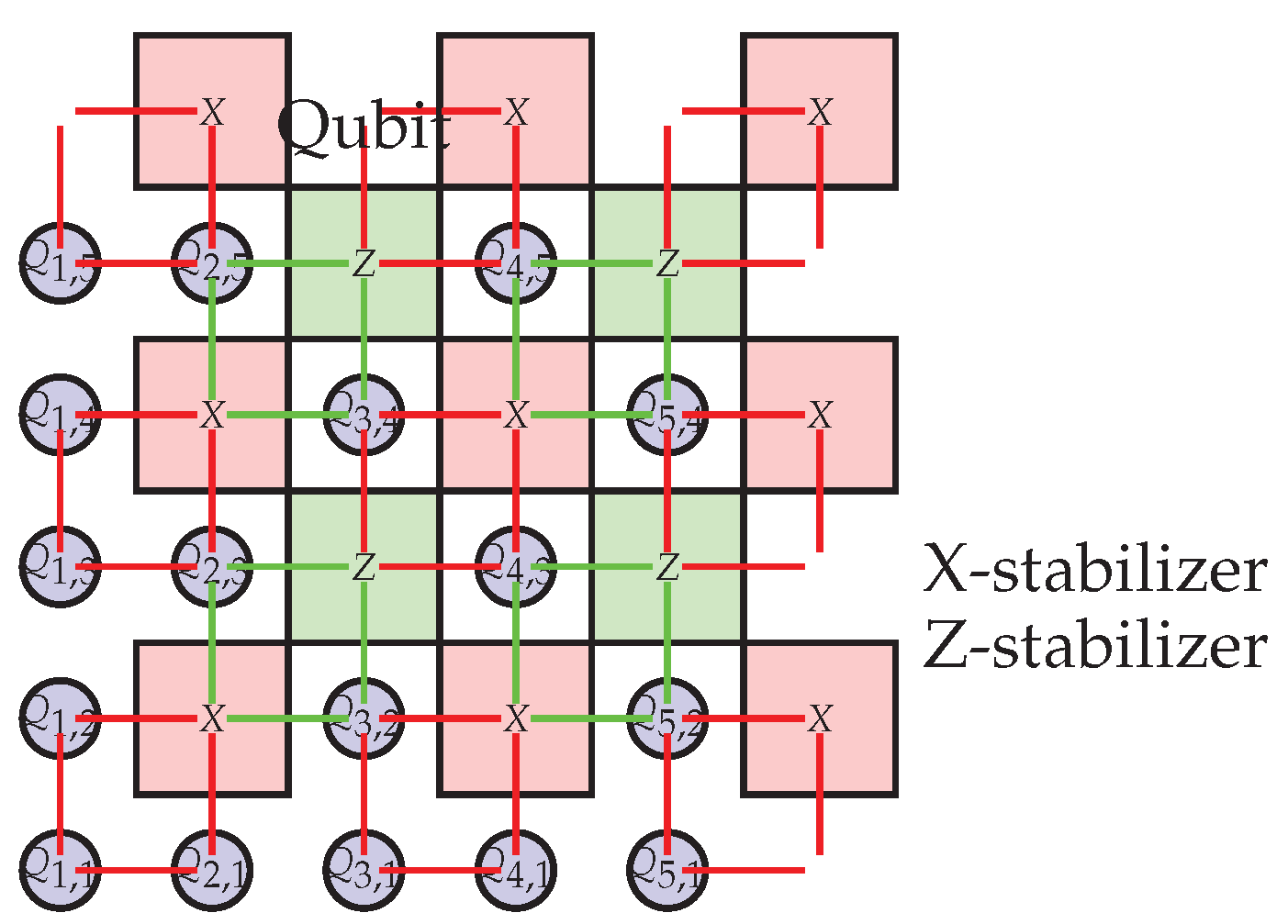
Figure 7.
Schematic of a surface code as a QLDPC code. Qubits (blue circles) are connected to X-stabilizers (red squares) and Z-stabilizers (green squares) in a local pattern.
Figure 7.
Schematic of a surface code as a QLDPC code. Qubits (blue circles) are connected to X-stabilizers (red squares) and Z-stabilizers (green squares) in a local pattern.
14. How to Use This Framework for Code Design
The GF(4)-symplectic framework provides a systematic methodology for quantum code design and analysis:
- Choose classical code(s): Select classical linear code(s) C with good parameters (rate, distance, efficient decoding)
- GF(4) representation: Encode C as a subspace of GF(4)n or use CSS construction with two classical codes
- Symplectic matrix construction: Convert to binary symplectic form
- Check commutativity: Verify , where
- Compute centralizer: Find kernel of the map
- Identify logical operators: Choose representatives from centralizer modulo stabilizers
- Calculate distance: Find minimum weight of non-trivial logical operators via enumeration or bounds
- Design syndrome extraction: Use flagged circuits based on stabilizer supports and weight
- Verify transversal gates: Check which Clifford gates preserve the code space by their symplectic action
- Simulate performance: Evaluate error correction threshold under realistic noise models
15. Conclusion: A Unified Pedagogical Foundation
This paper has presented a complete, constructive derivation of the Steane [[7,1,3]] quantum error-correcting code using a unified framework that connects GF(4) algebra, binary symplectic representation, and stabilizer formalism. Through explicit step-by-step development, we have demonstrated:
1. How GF(4) provides the natural algebraic language for Pauli operators modulo phases 2. How binary symplectic representation transforms quantum commutation into matrix multiplication 3. How classical Hamming codes directly yield quantum CSS codes via the symplectic construction 4. How all code properties—stabilizers, logical operators, distance, syndromes—follow from linear algebra 5. How transversal Clifford gates emerge from symplectic transformations 6. How fault-tolerant measurement circuits implement the algebraic structure 7. How this framework extends systematically to modern code families
The pedagogical value of this unified approach is substantial. By presenting quantum error correction as a coherent mathematical framework rather than a collection of disjoint techniques, we lower the barrier to entry for new researchers while providing experienced practitioners with a systematic methodology for code design and analysis.
Future work can build upon this foundation to explore more advanced topics, including:
- Non-CSS stabilizer codes using full GF(4) representations
- Topological codes as special cases of the symplectic framework
- Union-Find and other modern decoders in the binary representation
- Hardware-efficient implementations of the symplectic operations
The GF(4)-symplectic framework presented here serves not only as a tutorial on the Steane code but as a versatile foundation for understanding, designing, and implementing quantum error correction in practice.
Acknowledgments
The author expresses sincere gratitude to the quantum information research community whose pioneering work on stabilizer codes, fault-tolerant quantum computation, and algebraic coding theory provided the essential foundation for this unified exposition. Special acknowledgment is extended to the original developers of the GF(4) representation, symplectic formalism, and CSS construction methodologies. This pedagogical synthesis was developed at Sirraya Labs. The author acknowledges the research support and intellectual environment provided by Sirraya Labs that enabled the comprehensive presentation of this unified framework. Correspondence and inquiries: Amir Hameed Mir, Sirraya Labs, amir@sirraya.org.
Appendix A. Comprehensive Reference Guide for Quantum Error Correction
This appendix serves as a self-contained pedagogical reference for all key concepts, notation, and terminology used throughout the paper. Organized thematically, it provides both quick lookup and deeper understanding of the mathematical foundations of quantum error correction.
Appendix A.1. Fundamental Mathematical Structures
- Finite Field GF(2) ()
-
The binary field with two elements and operations:All binary linear algebra in this paper operates over GF(2).
- Finite Field GF(4)
-
Extension field with four elements where , defined by the irreducible polynomial :Complete arithmetic tables:
- Vector Space
- Set of all binary vectors of length n with component-wise addition modulo 2. Forms the foundation for classical linear codes.
- Binary Linear Algebra
-
Matrix operations performed modulo 2:
- Matrix addition:
- Matrix multiplication:
- Dot product:
Appendix A.2. Pauli Group Theory and Representation
- Single-Qubit Pauli Matrices
- The four fundamental operators:
- Pauli Group
- Single-qubit Pauli group including phases:
- Pauli Group
-
n-qubit Pauli group:Elements are tensor products of single-qubit Paulis with overall phase or .
- GF(4)–Pauli Isomorphism
-
Fundamental correspondence (modulo phases):
- Binary Symplectic Representation
-
Encoding Pauli (modulo phase):where for each qubit j:
- if P has X or Y on qubit j
- if P has Z or Y on qubit j
- Symplectic Form Matrix
- The matrix defining the symplectic inner product:where is the zero matrix and is the identity matrix.
- Symplectic Inner Product
- For , :
- Commutation Theorem
- Two Pauli operators P and Q commute if and only if .
- Operator Weight
- = number of qubits where P acts non-trivially (not as I).
- Operator Support
- = set of qubit indices where P acts non-trivially.
Appendix A.3. Classical Coding Theory Fundamentals
- Linear Code C
- A subspace of dimension k. Contains codewords.
- Code Parameters [
-
]
- n: block length (number of bits)
- k: dimension (number of information bits)
- d: minimum distance =
- Generator Matrix G
- matrix whose rows form a basis for C:
- Parity-Check Matrix H
-
matrix satisfying:Equivalently: .
- Syndrome (Classical)
-
For error :Used to detect and correct errors.
- Coset
- For linear code C and error e: .
- Syndrome Decoding
- Mapping syndromes to coset leaders (minimum weight errors).
- Hamming Weight
- = number of 1’s in binary vector v.
- Hamming Distance
- .
- Dual Code
- .
Appendix A.4. Stabilizer Quantum Error Correction
- Stabilizer Group S
- An abelian subgroup of not containing .
- Stabilizer Code
- The subspace:
- Stabilizer Generators
- Independent set that generate S.
- Code Parameters [[
-
]]
- n: number of physical qubits
- k: number of logical qubits =
- d: code distance = minimum weight of non-trivial logical operator
- Centralizer
- Set of Pauli operators commuting with all elements of S:
- Normalizer
- For stabilizer codes: .
- Logical Operators
- Elements of . Act non-trivially on encoded information.
- Codespace Dimension
- .
- Syndrome (Quantum)
- For error , measurement outcomes of stabilizer generators:
Appendix A.5. CSS Code Construction
- CSS Construction
-
Given two classical linear codes with :
- X-stabilizers: Generators from rows of (parity-check of )
- Z-stabilizers: Generators from rows of (parity-check of )
- Symplectic Stabilizer Matrix
- For CSS codes:
- Code Parameters
- For CSS code from and :
- Independent X and Z Correction
- CSS codes correct X and Z errors separately using classical decoders for and respectively.
Appendix A.6. The Steane [[7,1,3]] Code in Detail
- Classical Foundation
-
Hamming code:
- Parity-check matrix:
- Minimum distance: 3 (corrects any single-bit error)
- Perfect code: syndromes match 7 single errors + no error
- Stabilizer Generators
- From CSS construction using same H for both X and Z:
- Logical Operators
- Canonical choice:
- Syndrome Table
-
All 21 single-qubit errors produce distinct syndromes:
- Transversal Gates
Appendix A.7. Fault-Tolerant Quantum Computation
- Fault-Tolerant Gate
- Implementation where a single physical fault causes at most one error per encoded block, preserving error correction capability.
- Hook Error
- Dangerous error propagation in multi-qubit gates where one fault creates correlated errors on multiple data qubits.
- Flag Qubit
- Ancilla used to detect when a measurement circuit may have created correlated errors.
- Flagged Syndrome Extraction
- Measurement circuit that uses flag qubits to signal dangerous fault patterns.
- Ancilla States
-
Special states for measurement:
- , : Logical zero and plus states
- , : Physical ancilla states
- Fault-Tolerant Measurement Circuit
-
For X-type stabilizer :
- Pseudo-Threshold
- Physical error rate below which encoded computation has lower logical error rate than unencoded computation.
- Code Capacity Threshold
- Error rate threshold assuming perfect gates and measurements.
- Circuit-Level Threshold
- Error rate threshold including gate, measurement, and preparation errors.
Appendix A.8. Extension to Modern Code Families
- Subsystem Codes
-
Decompose Hilbert space as where:
- : Logical subsystem (protected information)
- : Gauge subsystem (not protected)
- Stabilizers act only on
- Gauge operators generate transformations within
- Quantum LDPC Codes
- Codes with sparse parity-check matrices (constant-weight stabilizers).
- Hypergraph Product
- Construction of QLDPC codes from two classical LDPC codes:
- Tanner Graph
-
Bipartite graph representation connecting:
- Variable nodes (qubits)
- Check nodes (stabilizer generators)
- Belief Propagation
- Iterative decoding algorithm operating on Tanner graph.
Appendix A.9. Complete Notation Reference
Table A1.
Comprehensive notation reference for quantum error correction.
| Symbol | Meaning and Usage |
|---|---|
| I, X, Y, Z | Single-qubit Pauli matrices |
| Pauli operator P applied to all n qubits | |
| Binary symplectic vector (u = X-part, v = Z-part) | |
| Symplectic inner product: u·v’ + v·u’ mod 2 | |
| Weight of operator P (non-identity components) | |
| Support set of operator P | |
| ⊕ | Addition modulo 2 (XOR) |
| GF(4) elements: , | |
| Binary field {0,1} | |
| Four-element field GF(4) = | |
| n-qubit Pauli group (including phases) | |
| Classical code parameters: length, dimension, distance | |
| Quantum code parameters: physical qubits, logical qubits, distance | |
| G | Generator matrix (classical) |
| H | Parity-check matrix (classical) or Hadamard gate (quantum) |
| M | Symplectic stabilizer matrix |
| S | Stabilizer group |
| X-type and Z-type stabilizer generators | |
| Logical X and Z operators | |
| C(S) | Centralizer of stabilizer group S |
| n-fold tensor product of Hadamard gates | |
| S | Phase gate: diag(1, i) |
| CNOT | Controlled-NOT gate |
| Computational and Hadamard basis states |
Appendix A.10. Common Constructions and Formulas
Table A2.
Useful formulas and constructions in quantum error correction.
| Construction | Formula/Procedure |
|---|---|
| Binary Symplectic Encoding | where for X/Y, for Z/Y |
| Syndrome Calculation | |
| CSS Code from C | , , |
| Centralizer Dimension | |
| Logical Qubit Count | |
| Code Distance | |
| Transversal Hadamard | |
| Transversal Phase | |
| Transversal CNOT | |
| Hamming Code H | Columns = binary numbers 1-7: |
| Steane Stabilizers | , , etc. |
Appendix A.11. Supplementary Examples and Exercises
Appendix A.11.11.1. Example: Verifying Steane Code Properties
- Verify that and commute using symplectic product.
- Show that has syndrome .
- Find the syndrome for error on the Steane code.
- Verify that maps to .
Appendix A.11.11.2. Example: General CSS Construction
Given classical code C with parity-check matrix:
Construct the corresponding CSS code and determine its parameters .
Appendix A.11.11.3. Exercise: Error Correction Capability
A code with distance can:
- Detect any error affecting qubits
- Correct any error affecting qubit
- Detect but not correct errors affecting 2 qubits
General rule: Code with distance d can correct errors.
Appendix A.12. Additional Resources and References
- Classical Coding Theory: MacWilliams and Sloane, "The Theory of Error-Correcting Codes"
- Quantum Information: Nielsen and Chuang, "Quantum Computation and Quantum Information"
- Stabilizer Formalism: Gottesman, "Stabilizer Codes and Quantum Error Correction"
- Fault Tolerance: Preskill, "Quantum Computing in the NISQ era and beyond"
-
Online Resources:
- arXiv:quant-ph for latest research
- QEC Zoo: errorcorrectionzoo.org
- PennyLane, Qiskit tutorials for implementation
Appendix A.13. Glossary of Acronyms
- QEC
- Quantum Error Correction
- CSS
- Calderbank-Shor-Steane (code construction)
- LDPC
- Low-Density Parity-Check
- GF
- Galois Field (finite field)
- MWPM
- Minimum Weight Perfect Matching (decoder)
- BP
- Belief Propagation (decoder)
- FT
- Fault-Tolerant
- CNOT
- Controlled-NOT gate
- NISQ
- Noisy Intermediate-Scale Quantum
- QLDPC
- Quantum Low-Density Parity-Check
References
- D. Gottesman, Stabilizer Codes and Quantum Error Correction, Caltech Ph.D. thesis, 1997.
- A. R. Calderbank and P. W. Shor, Good quantum error-correcting codes exist, Phys. Rev. A 54, 1098 (1996).
- A. M. Steane, Error correcting codes in quantum theory, Phys. Rev. Lett. 77, 793 (1996).
- A. Leverrier, J. A. Leverrier, J. Tillich, and G. Zémor, Quantum expander codes, Proc. IEEE FOCS, 810–819 (2015).
- P. Panteleev and G. Kalachev, Asymptotically good quantum and locally testable classical LDPC codes, Proc. ACM STOC, 375–388 (2022).
- C. Chamberland and M. E. Beverland, Flag fault-tolerant error correction with arbitrary distance codes, Quantum 4, 256 (2020).
- D. Poulin, Stabilizer formalism for operator quantum error correction, Phys. Rev. Lett. 95, 230504 (2005).
- A. A. Kovalev and L. P. Pryadko, Quantum Kronecker sum-product low-density parity-check codes with finite rate, Phys. Rev. A 88, 012311 (2013).
- J. Tillich and G. Zémor, Quantum LDPC codes with positive rate and minimum distance proportional to the square root of the blocklength, IEEE Trans. Inf. Theory 60, 1193–1202 (2014).
- A. G. Fowler, M. A. G. Fowler, M. Mariantoni, J. M. Martinis, and A. N. Cleland, Surface codes: Towards practical large-scale quantum computation, Phys. Rev. A 86, 032324 (2012).
Disclaimer/Publisher’s Note: The statements, opinions and data contained in all publications are solely those of the individual author(s) and contributor(s) and not of MDPI and/or the editor(s). MDPI and/or the editor(s) disclaim responsibility for any injury to people or property resulting from any ideas, methods, instructions or products referred to in the content. |
© 2025 by the authors. Licensee MDPI, Basel, Switzerland. This article is an open access article distributed under the terms and conditions of the Creative Commons Attribution (CC BY) license (http://creativecommons.org/licenses/by/4.0/).
Copyright: This open access article is published under a Creative Commons CC BY 4.0 license, which permit the free download, distribution, and reuse, provided that the author and preprint are cited in any reuse.


