
Submitted:
01 December 2025
Posted:
02 December 2025
You are already at the latest version
Abstract
Metadata extraction from the labels of natural history collections is a pivotal task for the online publication of digitized specimens. However, this is an extremely time-consuming task, given the estimated number of specimens in natural history collections (more than 2 billion specimens worldwide, of which ca. 400 million are herbarium specimens). Thus, automated data extraction from digital images of specimens and their labels is an application where state-of-the-art computer vision techniques could successfully be applied. The task of extracting information from the labels of herbarium specimens is made of three steps: text segmentation, multilingual/handwriting recognition, and data parsing. The principal bottleneck in the process is the limitation of Optical Character Recognition (OCR). This study aims to explore how to transfer the general knowledge present in multimodal Transformers into the specific sub-task of herbarium specimen label digitization. This would result in an easy-to-use, end-to-end solution, which strives to get rid of the bottleneck of classic OCR systems, while allowing for higher flexibility to adapt to different label formats. Donut-base, a pre-trained visual document understanding (VDU) transformer, was the base model selected for fine-tuning. A dataset from the University of Pisa was used as a test bed. The initial attempt achieved an 85% accuracy computed by the Tree Edit Distance (TED), demonstrating that fine-tuning is a feasible solution. Cases with low accuracies were also investigated to highlight flaws in the approach. Specimens with more than one label, especially when a mix of different handwriting and typewritten information were present, are the most difficult to deal with, and approaches aimed at targeting these weaknesses are discussed.
Keywords:
artificial intelligence
; biodiversity
; digitization
; multimodality
; vision-language transformer
1. Introduction
Natural history collections (NHCs) host large amounts of specimens collected since the 17th century. The total amount of specimens worldwide is estimated at more than 2 billion [1]. Herbaria, which are natural history collections of dried plant specimens, are estimated to host ca. 400 million specimens worldwide [2]. Each specimen normally has one or more labels reporting metadata such as scientific name, date and locality of collection, collector, etc. These data are pivotal for understanding the evolution of biodiversity [3], and for forecasting its changes in the future, other than for a wide array of other research topics [4,5].
The mobilization of specimen data utilizing digitization is thus particularly relevant [6,7,8]. While several digitization efforts are made manually, massive and industrialized workflows to improve digitization efficiency have been experimented on botanical [9] and, more recently, entomological collections. In general, modern digitization efforts follow an image-to-data workflow [10]. This consists of taking digital images of specimens and their labels, from which metadata are transcribed. This allows for a limited manipulation of the specimens, which, being biological objects, are particularly prone to deterioration [11,12]. Label data are then usually published in “global” repositories such as the Global Biodiversity Information Facility (GBIF) organized with a common standard, such as Darwin Core [13].
To further increase the efficiency of digitization actions, the process of metadata extraction - which is quite labor-intensive [14,15] - through computer vision for automated metadata extraction is being investigated [16,17,18,19]. Since standard OCR was seen as the only tool able to recognize printed and handwritten strings on labels, most previous attempts focused on combining an OCR system and a natural language processing (NLP) algorithm, the former to get unstructured information out of the image, the latter to tackle Name Entity Recognition (NER). Those systems normally provide an interface where a human operator can correct or enter missing data from scratch. HERBIS19 [20] and SALIX20 [16] are representatives of such a design. Simple OCR approaches can speed up data entry supporting label transcription, but they cannot overcome limitations related to lackluster label quality [16]. Indeed, these approaches still require motivated manpower for day-to-day supervision of their output, since they are not - at the current state of the art - reliable enough. With the advancement of OCR technologies and the emergence of Large Language Models (LLMs), however, it was possible to create new integrated workflows. “Publish First” [21] is an example of this novel approach. These approaches, however, rely on fully developed services accessible by APIs, often managed by external entities, which can be commercial companies. Thus, several drawbacks could arise, the first being that it is usually impossible to interpret and improve all the components in the workflow relying on external APIs. Except for a satisfactory result obtained in a pipeline which used external services, like GPT-4, no other explicit explanation supporting service choice or further analysis of worst cases can be provided [21]. Furthermore, data privacy and confidentiality often cannot be properly ensured when using LLMs hidden behind APIs, since they may store or misuse private or sensitive data, thus exposing users to the risk of private data leakage [22].
A fully trainable and adjustable information extraction (IE) model composed of only open-source solutions is, however, still lacking. This challenge has been partly addressed with the development of a novel automated label data extraction and database generation system from herbarium specimen images using OCR and NER [23]. This workflow uses the SpaCy python package for NER parsing after the text has been extracted through the Google Cloud Vision OCR service. While this NER parsing solution is promising and innovative, the OCR service it uses is not flexible enough to tackle the complexity arising from different label formats. An OCR can detect and recognize the portions of text in a document but not understand them and their content based on their position in the image. Google’s OCR is also a closed-source service, thus limiting users in its tailoring to their needs. With the advent of new techniques in NLP and Computer Vision (CV), driven by the rise of Transformer [24], however, an alternative approach leveraging their power and versatility might be developed. Thanks to Transfer Learning [25], Large Vision-Language Models (LVLMs), trained with huge sets of general data, can be fine-tuned for specific sub-tasks targeting fewer data. Several Language-Vision Transformers were developed, since [26] proposed the Multimodal Transformer (MulT), a cross-modal attention mechanism based on a Transformer, capable of decreasing the stress of explicit data aligning. These approaches had astonishing performances, as evidenced by [27] in the development of TrOCR and [28] in the development of Donut. Language-vision models include both an image encoder and a text decoder. They are trained to recognize all texts in images and to extract information, but with some differences. TrOCR takes text lines as input and is not suitable for NER out of the box, while Donut is better suited for an IE task [27].
This research aims at describing the first successful fine-tuning of Donut [28] to automatically extract information from herbarium specimen labels and to arrange them in the concepts of the metadata standard scheme Darwin Core [13], which is internationally adopted for the interoperability of these data. This is the first real-world use of the latest multimodal Transformer to effectively facilitate the difficult tasks of digitizing herbarium specimens.
2. Materials and Methods
2.1. Dataset
This study was carried out on a dataset of digitized specimens from the Herbarium of the University of Pisa (international acronym PI). The dataset comprises 55,089 specimens, which were digitized and published online using the online database JACQ Virtual Herbaria (), a continuously developing consortium of virtual herbaria located in Vienna [29,30]. Most of the specimens come from a recently completed digitization project devoted to the Herbarium Guadagno [31]. The images are in JPEG format, while the metadata (derived from a manual transcription of the original labels in each specimen) are organized in a spreadsheet, in which each row represents a single specimen. The dataset hosts digital specimens from 97 countries, which were collected in the span of two centuries. From the spreadsheet, the following data were retained and used as ground truth in the fine-tuning process of the algorithm: Original scientific name, collection date, collection locality and elevation. Each record must be a pair of a specimen image and a ground truth. After cleaning images missing ground truths, the final dataset contained 45,951 specimens. Ground truths were converted to JSONL (), a data format that can be transformed into text for the model training. It should be noted that sometimes the ground truth provided with the images does not always correspond to the actual text on the label(s). This is mostly due to updates in the scientific nomenclature (i.e., when the original name is replaced with a modern accepted name, without updating the original label), or to partial transcription of other information.
2.2. Base Model Selection
Given the limited amount of data in the dataset, instead of training a model from scratch, we relied on a transfer learning technique called fine-tuning. This allowed us to adapt a model to a specific and narrow domain with minimal additional training data effort. Thus, a base model pre-trained on an extensive large-scale dataset for general knowledge has been selected. Candidate base models should be able to support multiple languages and complex label formats, without the limitation given by OCR. Performance on mainstream benchmarks CORD [32], a dataset containing 10K Latin alphabet receipt images, was identified as a good criterion to compare the capabilities of different base models (see Table 1).
Donut was selected as the base model for fine-tuning. While BERT can be used as a baseline for any IE task, since it is a model adaptable for multiple language tasks, it has no component to recognize texts from images. Thus, when used for IE it must rely on an external OCR engine. On the other hand, Donut was specifically designed to recognize text within pictures, making it a more suitable choice. As far as TrOCR is concerned, while it uses an encoder-decoder architecture like Donut, it requires “text-line” images as input [27]. These must derive from a preprocessing image segmentation phase, in which the original image is cropped into several portions, each one containing a line of text only. Thus, it can only extract text from images but can’t be used to parse the complex structure of the data. Donut is the only OCR-free model capable of extracting information from documents without requiring any preprocessing before feeding images into the model. Furthermore, it is trained on a multi-language dataset, which includes Chinese, Japanese, Korean, and English.
2.3. Dataset Preprocessing
In our proposed multimodal Transformer, the pre-trained image encoder and text decoder were fine-tuned with a set of pairs consisting of a specimen image and the corresponding ground truth. The following data preparation steps were applied before the fine-tuning:
- Image resolution was decreased to avoid excessive computational requirements, as well as to test the effect of image resolution on the output of the model. Datasets with images at three different resolutions (600×800, 960×1280, and 1200×1600) were prepared for testing the IE performance of the model.
- The ground truth was structured in a JSONL format, where the keys are special tokens which were previously added to the model tokenizer, according to [28].
Furthermore, when the pre-trained model is used at inference time, the text decoder begins generating from a standard start token “<s>”. Thus, a task-specific prompt token “<s_herbarium>” was added as the start of the sequence for the fine-tuned model. This prompt token is used to replace the start token “<s>” in the general model inference.
2.4. Experiment Environment Setting up
Donut was fine-tuned on the CINECA () HPC facility, and specifically the Leonardo Booster module. The environment was a single computer node equipped with one Intel Xeon 8358 CPU with 32 cores running at 2.6 GHz, four NVIDIA Ampere A100 GPUs with 64GB graphics memory, and 512 GB RAM. The batch size selected varied in each fine-tuning depending on image resolution (See Table 2). All other hyperparameters, including precision, optimizer, and learning rate are following the indications of the Donut paper [28]. The code of the fine-tuned model (named HeR-T - Herbarium label Recognition-Transformer) and details of settings are available at GitHub: HeR-T: Herbarium specimen label Recognition Transformer.
2.5. Fine-Tuning
Fine-tuning is effective when the target dataset available for the re-training is significantly smaller than the base dataset used for the pre-training [37]. Donut, the selected base model, was pre-trained with 2 million synthetically generated images, which is indeed much larger than our 45,951 specimen images target dataset.
Besides that, when the base task and target task are similar, the transferability of features can be enough to enhance the efficiency of fine-tuning [37]. In our case, the target task – IE from specimen labels – can be seen as a sub-task of a broader text recognition task, which is the base task of Donut. Thus, the learned features of Donut can be largely transferred, enabling effective fine-tuning. In our research, we performed a full fine-tuning without freezing any layers.
Regarding the loss function used for fine-tuning, we inherited the cross-entropy of Donut. The prediction of a token can thus be interpreted as a classification problem, which is based on the conditioned distribution of the image and the context from previous tokens [28].
However, Large Vision-Language Models (LVLM) such as Donut are known to overfit when the target dataset for fine-tuning is not large enough [37]. Thus, early stopping was implemented in the fine-tuning process to avoid overfitting. Whenever the Tree Edit Distance (TED) accuracy on the validation set was equal or higher than the score in the previous validation, the fine-tuning process was interrupted (early stopping). During the fine-tuning phase, the tree edit distance (TED) accuracy (see next section) on the validation set was evaluated every 25% of one training epoch was (e.g., four validations per training epoch). Because of fluctuations in model performance during the training, premature stopping could occur before the model was properly trained. To mitigate this problem, we introduced a “patience” parameter of 7, meaning the model was willing to wait for seven consecutive validations before stopping.
2.6. Evaluation: TED Accuracy
where gt, pr, and Ψstand for ground truth, prediction, and empty trees respectively [28].
For brevity we will refer to the score (1) as TED accuracy. Given the tree structures, which represent predicted text sequences, the TED accuracy (1) is based on the distance TED (pr, gt) between the ground truth and the predicted sequence, and the distance TED (Ψ, gt) between the ground truth and the empty tree. The fewer edits the prediction requires to align with the ground truth, the closer to 1 the TED will be. If compared with the traditional F1 score [39], which only counts the prediction’s words overlapping with the ground truth, TED accuracy can consider the structure of the predicted text sequence, as well. This formulation as an evaluation metric was adopted by [28], as well as in other IE approaches [33,40]. Thus, we adopted TED accuracy both as a benchmark and as the evaluation metric for the early stopping during fine-tuning.
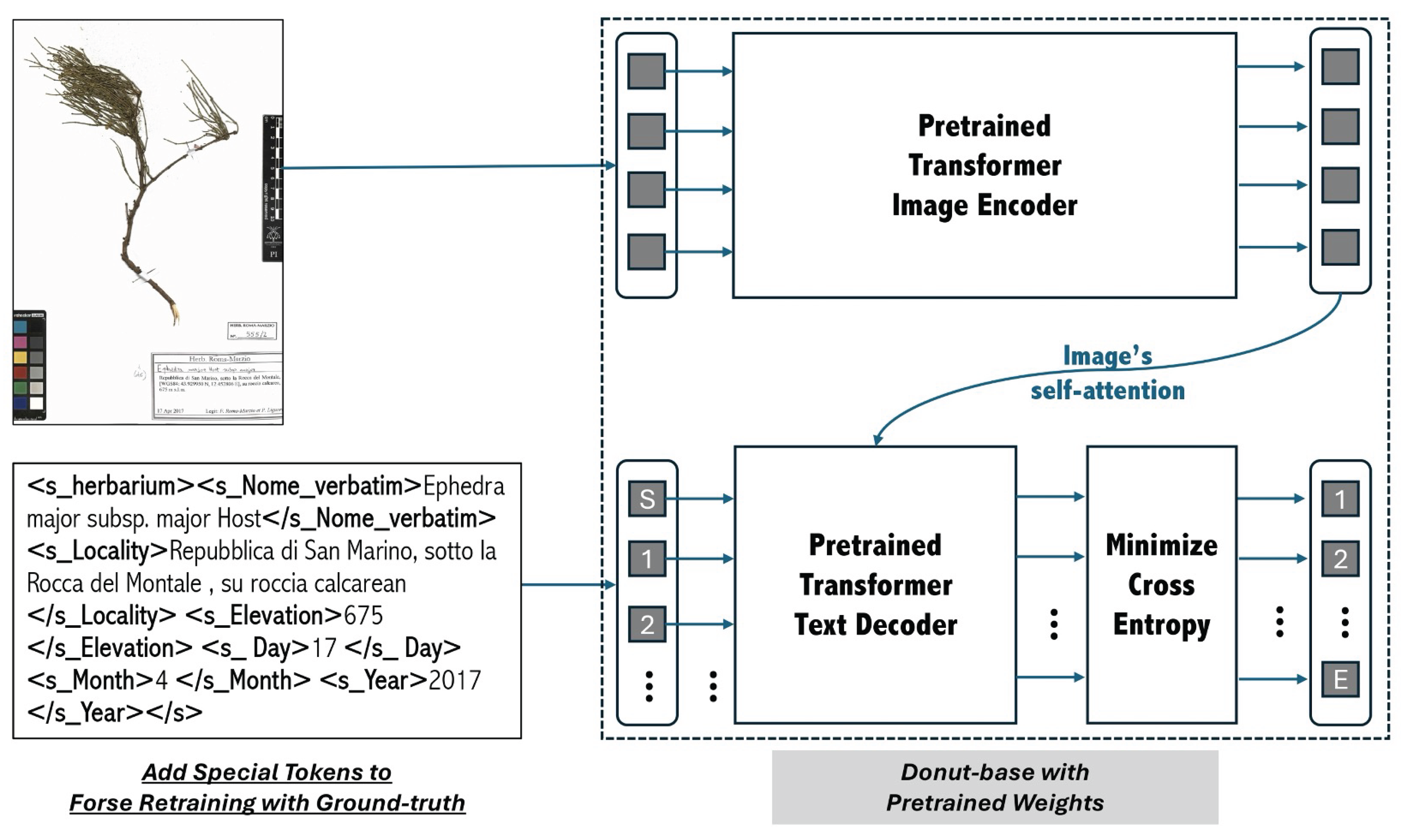
Figure 1.
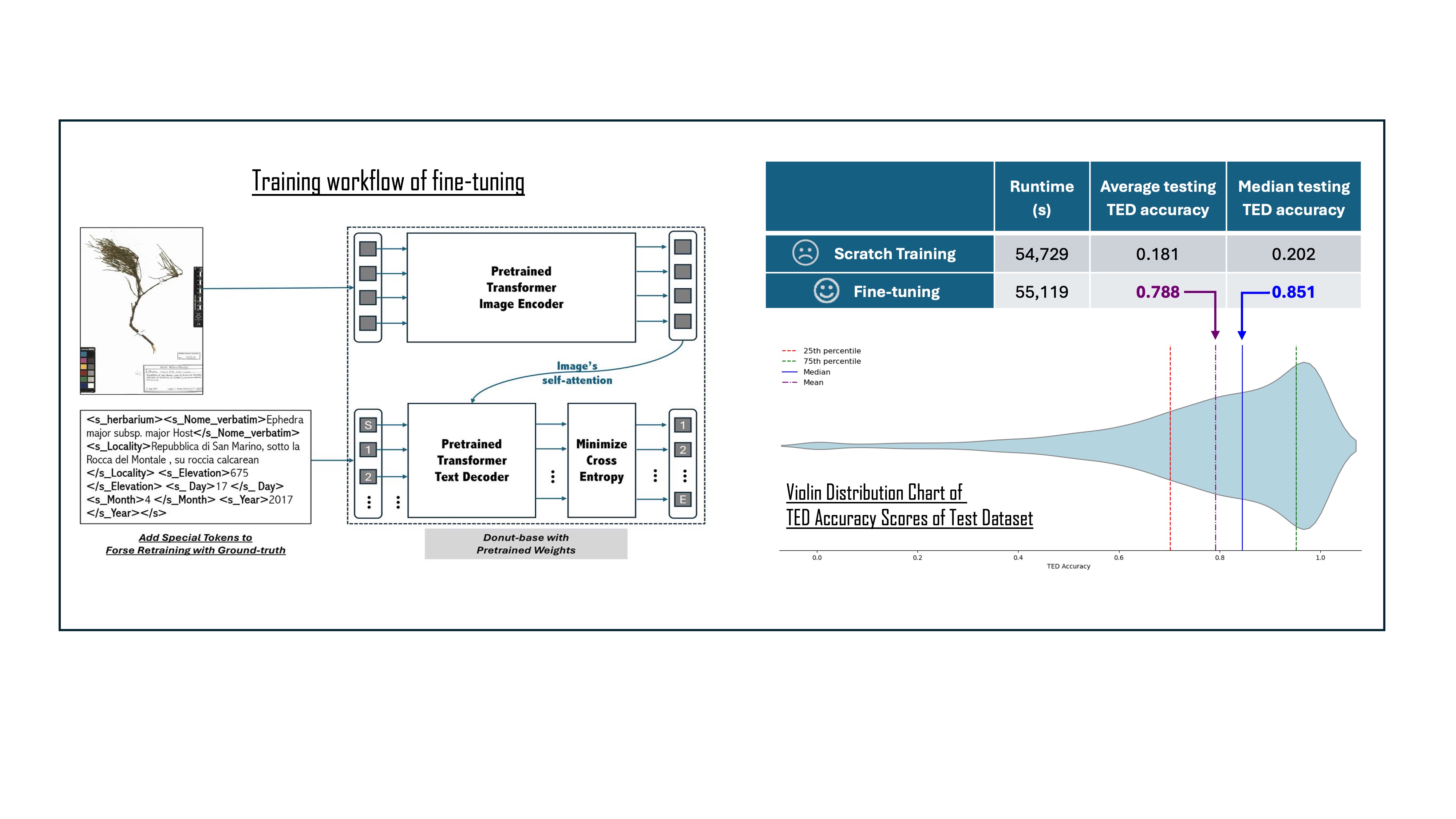
Fine-tuning workflow with a set of pairs of specimen image/ground truth. Images are converted in RGB and passed as input to the pre-trained encoder for the image’s self-attention. The output of the encoder is passed to the pre-trained decoder for cross-attention, matching the image with the parsed ground truth. The fine-tuning minimizes the cross-entropy loss function and forces the model to generate the same output as in the ground truth.
Figure 1.
Fine-tuning workflow with a set of pairs of specimen image/ground truth. Images are converted in RGB and passed as input to the pre-trained encoder for the image’s self-attention. The output of the encoder is passed to the pre-trained decoder for cross-attention, matching the image with the parsed ground truth. The fine-tuning minimizes the cross-entropy loss function and forces the model to generate the same output as in the ground truth.
3. Results
Three attempts of fine-tuning were conducted with different image resolution setups, and all models’ performances were assessed on the same test image dataset with corresponding resolutions: 600×800, 960×1280, and 1200×1600. As shown in Table 3, TED accuracies increase with the image resolution. Thus, the 1200×1600 resolution was adopted for further inference as it achieved the best TED accuracy median score.
To test whether the pre-trained Donut transferred the effective learning process to the IE task of extracting information from specimen labels, the model was also trained from scratch with images at 1200×1600 and the same parameters used in the fine-tuning. For comparison, the scratch training was stopped after five epochs, which is the same as the training epoch in the fine-tuning with 1200×1600 images.
After an initial training from scratch of five epochs without early stopping, the process evidenced a limited improvement in both training loss and evaluation score. In Figure 2, both training from scratch loss curves remain high, if compared with fine-tuning. A detailed comparison is reported in Table 4.
In Table 3 and Table 4, even if median and average TED accuracy have margin to 1, which is the max TED accuracy score, the evaluation has been satisfactory considering the TED accuracy distribution in the test dataset. In more than 75% of the cases, the TED accuracy score is higher than 0.702 (Figure 3), and in 25% of the cases it is higher than 0.952.
The lower performances, however, are not necessarily errors in the identification of the text. They might represent “false negatives”, often due to differences between the ground truth and the actual text on the labels. Table 5, Table 6, Table 7 and Table 8 showcase several examples of different performance, from the lowest to the best. The images in the tables are available also as supplementary materials (Figure A1, Figure A2, Figure A3, Figure A4, Figure A5, Figure A6, Figure A7 and Figure A8). In the tables the text in green is the portion which is identical in the ground truth and in the prediction, while in red the portion which differs.
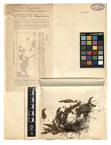
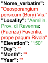
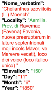
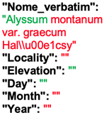
In Table 5 there are two specimens for which the accuracy score is 0. In the first case, the fine-tuned Donut correctly extracted the scientific name, though only partially as it missed the authorities and the variety. However, it is worth noting that the ground truth provided for this specimen differs from what is literally written on the label. This is because the name in the dataset was updated due to recent nomenclatural changes. In fact, one of the synonyms listed in the label is the currently accepted name of the taxon, while the name which was used on the label was not valid since it is a nomen nudum (i.e., not validly published), and should be discarded.
The extracted gathering locality is partially accurate, but the subsequent information in Latin, which in the image is partly hidden by the envelope of the specimen, is not extracted correctly. Thus, even if the TED accuracy score is 0, the algorithm extracted correctly at least part of the information. Thus, this case could be listed among the “false negatives”. In the second case of Table 5, the TED accuracy of 0 is due to the presence of two specimens on a single sheet, and to the presence in the ground truth of the transcription of the first one alone. Donut, on the contrary, extracted (correctly) the information from the second label alone. If the latter were considered, the TED accuracy would have been close to 1. However, Donut missed one of the two labels.
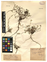
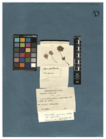
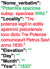
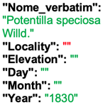
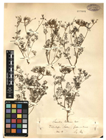
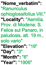
In Table 6, there are two examples of poor performance (TED accuracy ca. 0.2). In the first case, the presence of three labels (instead of the classical one) could be the cause of the poor performance. Donut extracted the scientific name (while missing the variety) from the label at the bottom, while took the year of gathering from the second one. It did not extract other information, such as the gathering locality. The ground truth, however, is not corresponding to one label alone. The scientific name was taken from the third label, but is not written correctly, since the authority (Willd.) should be placed after the binomial (Potentilla speciosa), and not after the variety (var. speciosa). Even the ground truth took the gathering date from the second label, together with the locality.
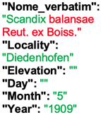
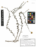
In the second case, Donut extracted a scientific name which is correct only as far as the genus is concerned (Scandix), while the species and authority are incorrect. The locality of collection was extracted entirely, while in the ground truth, it was only partially transcribed. However, Donut probably interpreted the text incorrectly, which was not transcribed in the ground truth. The gathering year is correct.
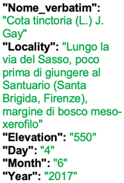
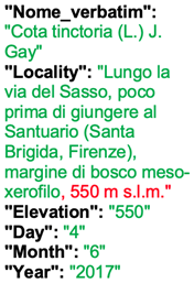
In Table 7, there are two examples in which the TED accuracy score was higher than 0.8. In these cases, the discrepancies between the predicted text and the ground truth are slight, if not irrelevant. In the first example, Donut predicted perfectly the content of the label, the only difference being in the inclusion of the altitude in the locality. The altitude is repeated in its concept as well. Thus, this is not an error in recognition, but in the organization of the output.
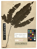
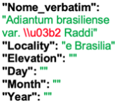
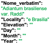
The second case is quite interesting. While the score in TED accuracy is lower than 1, the error is due to the presence of a typo in the ground truth. Donut predicted the text correctly, but for an error which is also present in the ground truth, i.e., the string of the scientific name, in which the authority (Raddi) is misinterpreted as the variety. In fact, while on the label the scientific name is written correctly (Adiantum brasiliense Raddi) and it is followed by the string “var.?”, which indicates that the specimen is probably a variety of the nominal species, the variety itself still lacks a proper identification. In both cases, anyway, the performance is satisfactory.
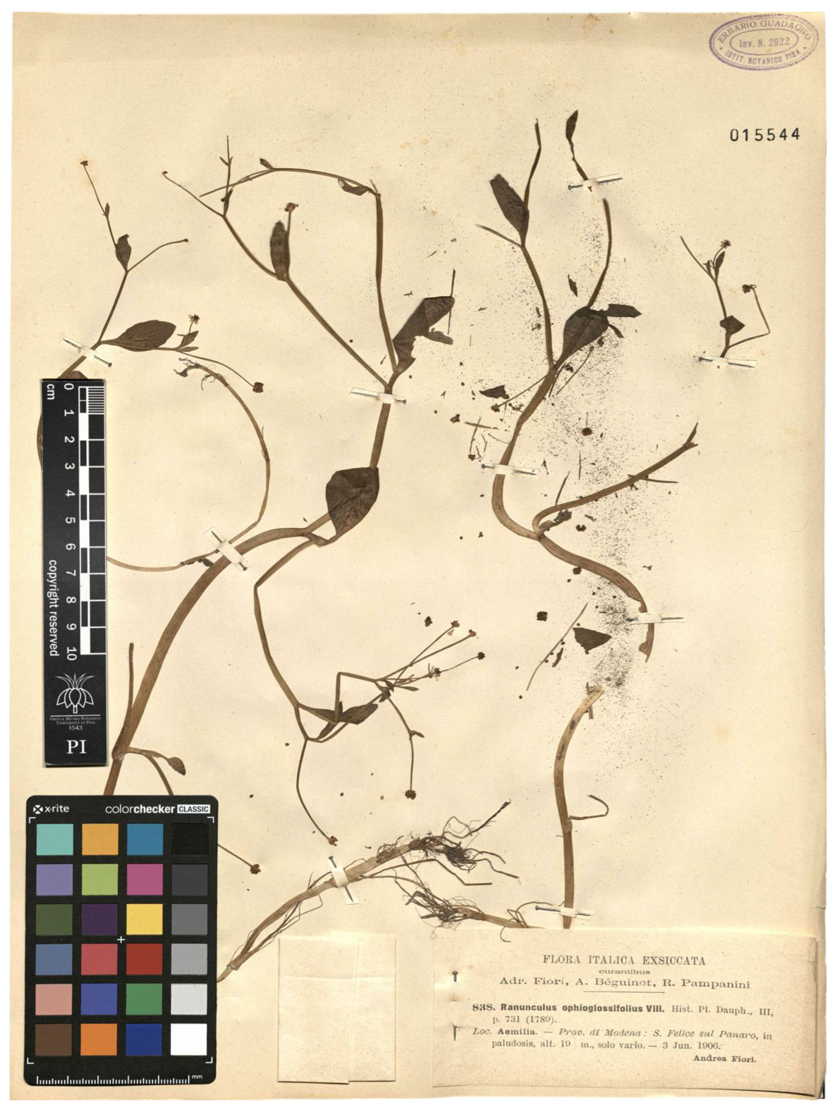
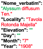
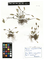
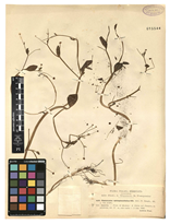
Table 8 displays some examples of a perfect TED accuracy score (1.0). In both cases, the prediction is exactly the same as the ground truth, which is the correct transcription of the contents of the label. While the first specimen has a handwritten label, the second is typewritten. In both cases one label alone is present on the herbarium sheet, which hosts a single specimen (the ideal scenario).
4. Discussion
Extracting metadata from natural history collection specimens is a challenging task, which calls for a relevant effort [14,15] if carried out manually. Thus, several attempts have been made to automate at least partially the process thanks to the use of OCR solutions, or by coupling an OCR with an NLP algorithm [16,17,18,19,20,21] take full advantage of the emergence of LLMs, creating integrated workflows. However, most of these examples rely on APIs managed by external entities, thus leading to several drawbacks, especially related to the lack of customizing and fine-tuning opportunities. The development of a fully customizable and adjustable IE approach could be seen as a step forward. [23] explored this solution by coupling a customizable SpaCy Python package for NER parsing with the Google Cloud Vision OCR service. However, this approach still lacks customization and fine-tuning opportunities as far as the OCR service is concerned.
Thus, we tried a novel approach to the problem by taking advantage of Transfer Learning [25], which allows to fine-tune LVLMs that have been pre-trained with huge sets of general data. Among the different possible solutions, we adopted Donut [27]. If compared to training a model from scratch, fine-tuning a pre-trained LVLM yields substantial performance improvements. A pre-trained LVLM as Donut, even if trained for more general-purpose tasks, is trained on datasets which are far larger than any domain-specific dataset. In the case of natural history specimens, a dataset should consist of images coupled with their metadata transcribed verbatim (the ground truth). Given the amount of images and data required, training from scratch a model for performing on this specific domain could be quite difficult. In our experience, training from scratch was ineffective if compared to the fine-tuning, especially at our dataset size. The fine-tuning process took less time and provided far better results, with a TED of 0.910 compared to 0.629 in the best-case scenario of training from scratch. Another issue related to training from scratch, other than the size of the training set, is related to the quality of the data. Existing domain-specific datasets produced by digitizing natural history collections sometimes do not contain the actual ground truth, but metadata which are derived from the ground truth. As an example, in some datasets, the localities of gathering of the specimens are not reported as they are written on the label, but homogenized according to some gazetteer, or toponymic database. In other cases, the scientific names are corrected, if they were written incorrectly on the label (e.g., without the authorities, or abbreviated), or even updated to the last nomenclatural updates (without updating the names written on the labels). Similar issues were also present in the dataset we adopted for the fine-tuning of Donut in this research.
The fine tuning allowed for quite satisfactory results (Figure 3). The median testing TED accuracy (0.851) highlights that the predictions of the fine-tuned Donut are generally quite close to the ground truth, and (Table 5 and Table 6) often a poor TED accuracy is not due to actual errors in the prediction, but in differences between the ground truth and the actual texts on the specimens’ labels (“false negatives”). The poorer performances are in general due to a) more than one label on the same herbarium sheet, often related to the presence of more than one specimen, and/or b) very poor handwriting. The metadata of specimens with one label are normally correctly predicted, even if the label is handwritten. In modern collections, this is mostly the case, while herbarium sheets with more than one label are rare. Thus, this approach could be potentially applied successfully to the digitization workflow for herbarium specimens. Further investigation is necessary for understanding the replicability of this approach on other natural history collections. However, wherever labels are visible in digital images, the replicability of this approach is potentially feasible.
While in this experience we adopted Donut as a base model for fine-tuning, a similar approach can be applied to any general-purpose LVLM. Since LVLMs are evolving at an incredibly fast pace, novel LVLMs could demonstrate better performance in the same domain than the relatively “old” Donut.
Author Contributions: Jacopo Zacchigna
Conceptualization, Methodology, Software, Writing – Original Draft, Writing – Review & Editing; Weiwei Liu (Corresponding Author): Methodology, Software, Investigation, Formal Analysis, Writing – Original Draft, Writing – Review & Editing; Felice Andrea Pellegrino: Supervision, Writing – Original Draft, Writing – Review & Editing; Adriano Peron: Supervision, Writing – Original Draft, Writing – Review & Editing; Francesco Roma-Marzio: Data Curation, Resources; Lorenzo Peruzzi: Data Curation, Resources, Writing – Review & Editing; Stefano Martellos: Supervision, Investigation (Herbarium Specimen Analysis), Validation, Writing – Review & Editing, Resources (Biodiversity Expertise).
Acknowledgments
The authors are grateful to CINECA for allowing the use of their HPC facilities in the framework of the project IsCb8_HeR-T (2024-2025).
Appendix A. Original Specimen Images in Table 5, Table 6, Table 7 and Table 8
Figure A1.
Upper image, Table 5.
Figure A1.
Upper image, Table 5.
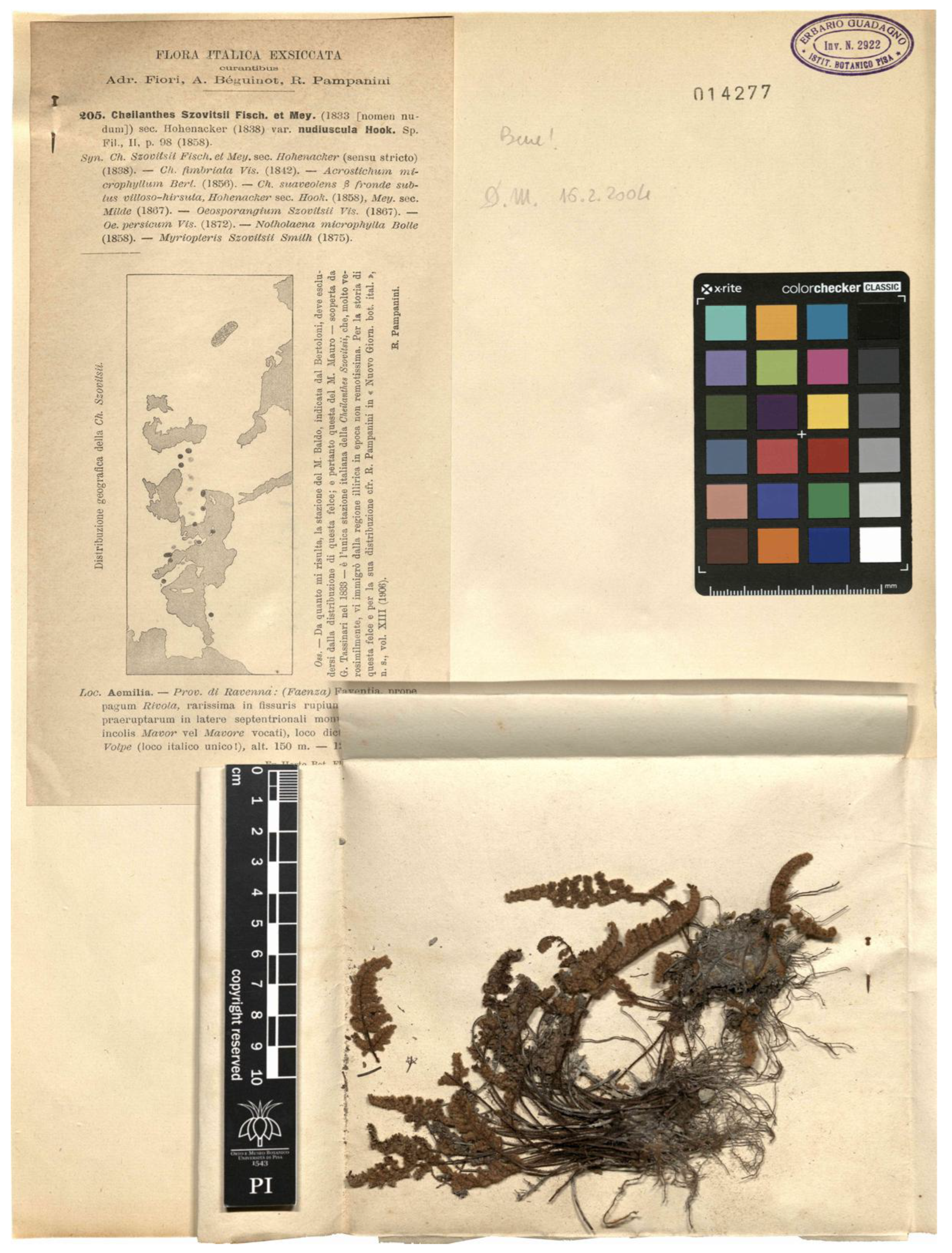
Figure A2.
Lower image, Table 5.
Figure A2.
Lower image, Table 5.
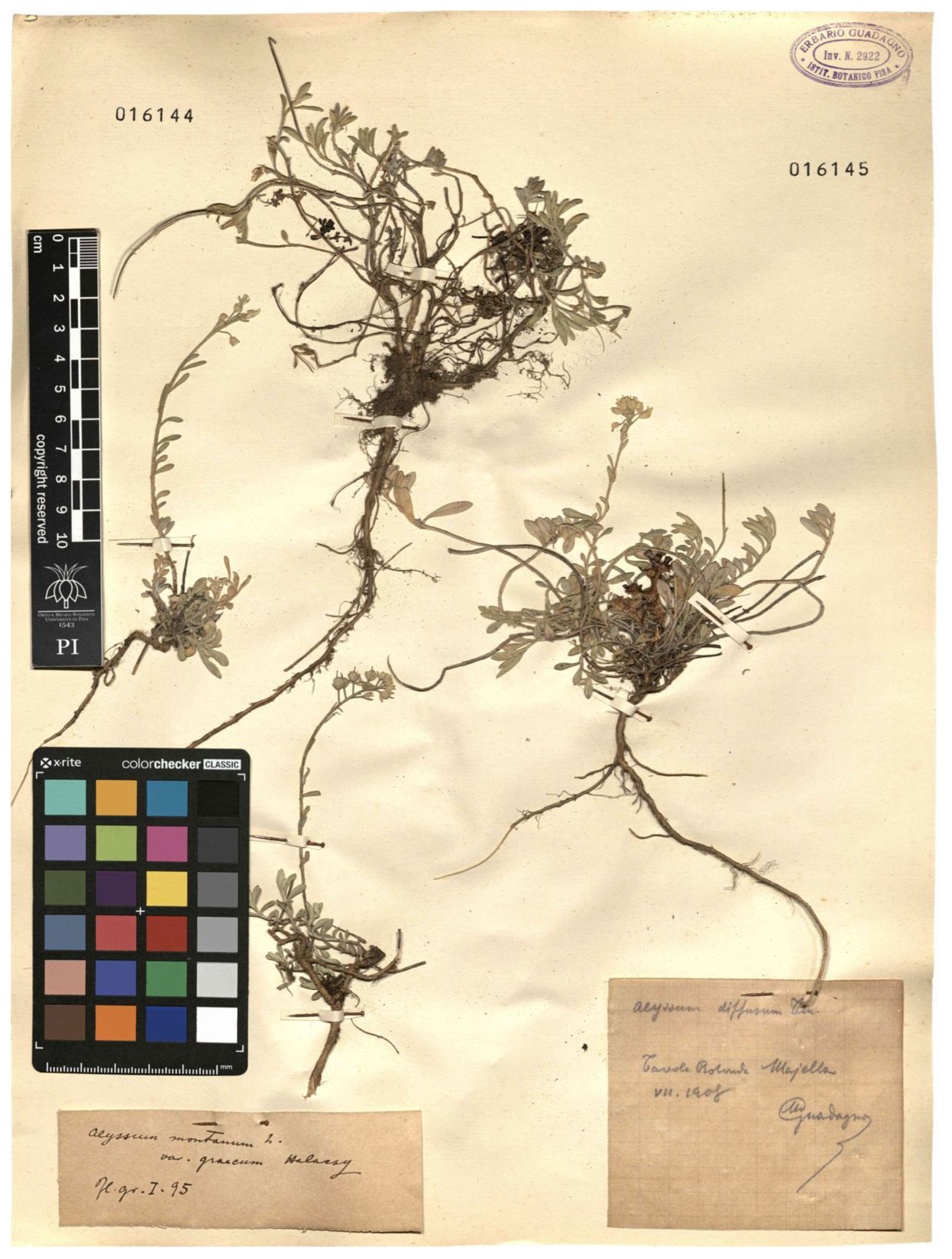
Figure A3.
Upper image, Table 6.
Figure A3.
Upper image, Table 6.
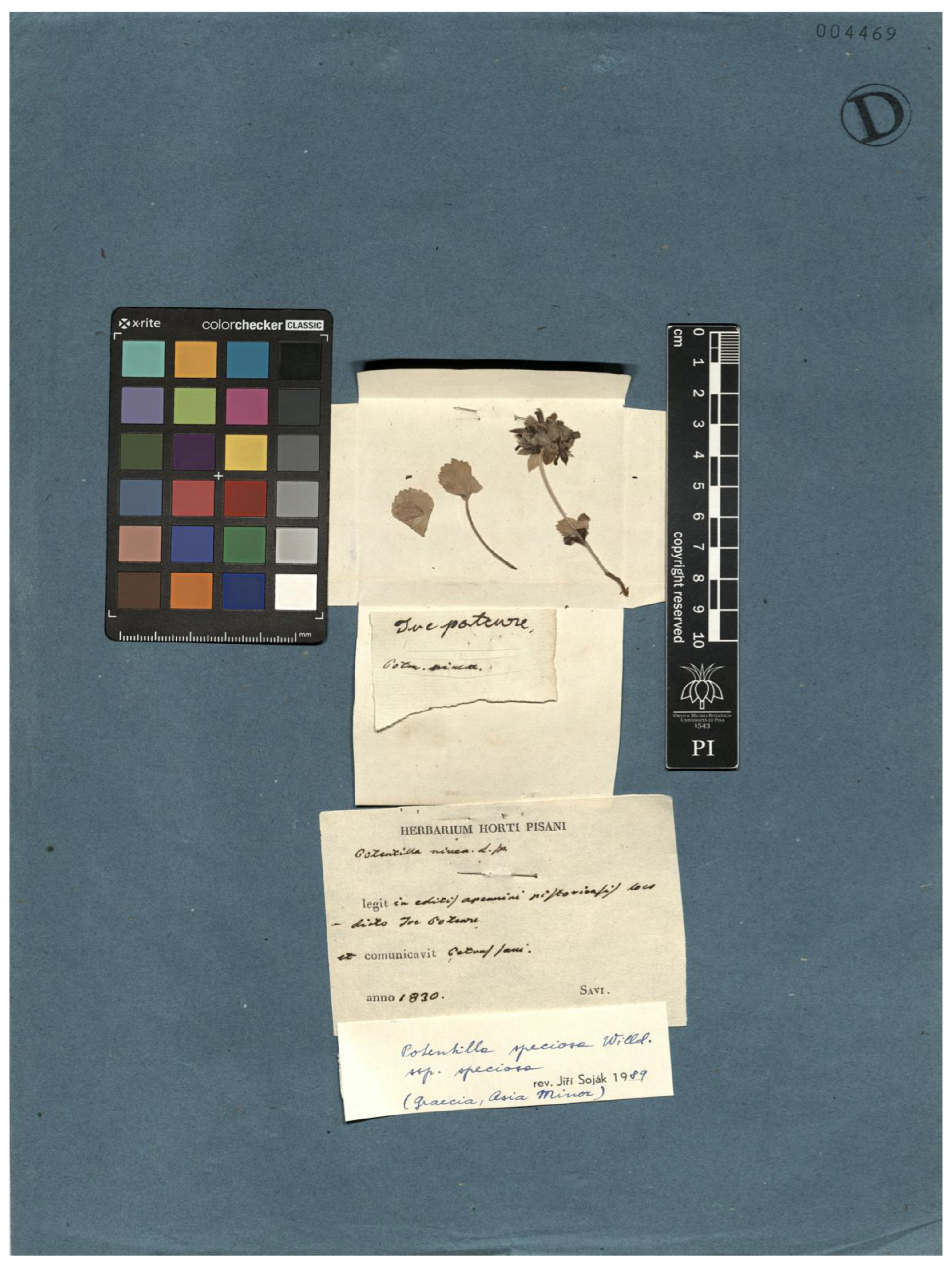
Figure A4.
Lower image, Table 6.
Figure A4.
Lower image, Table 6.
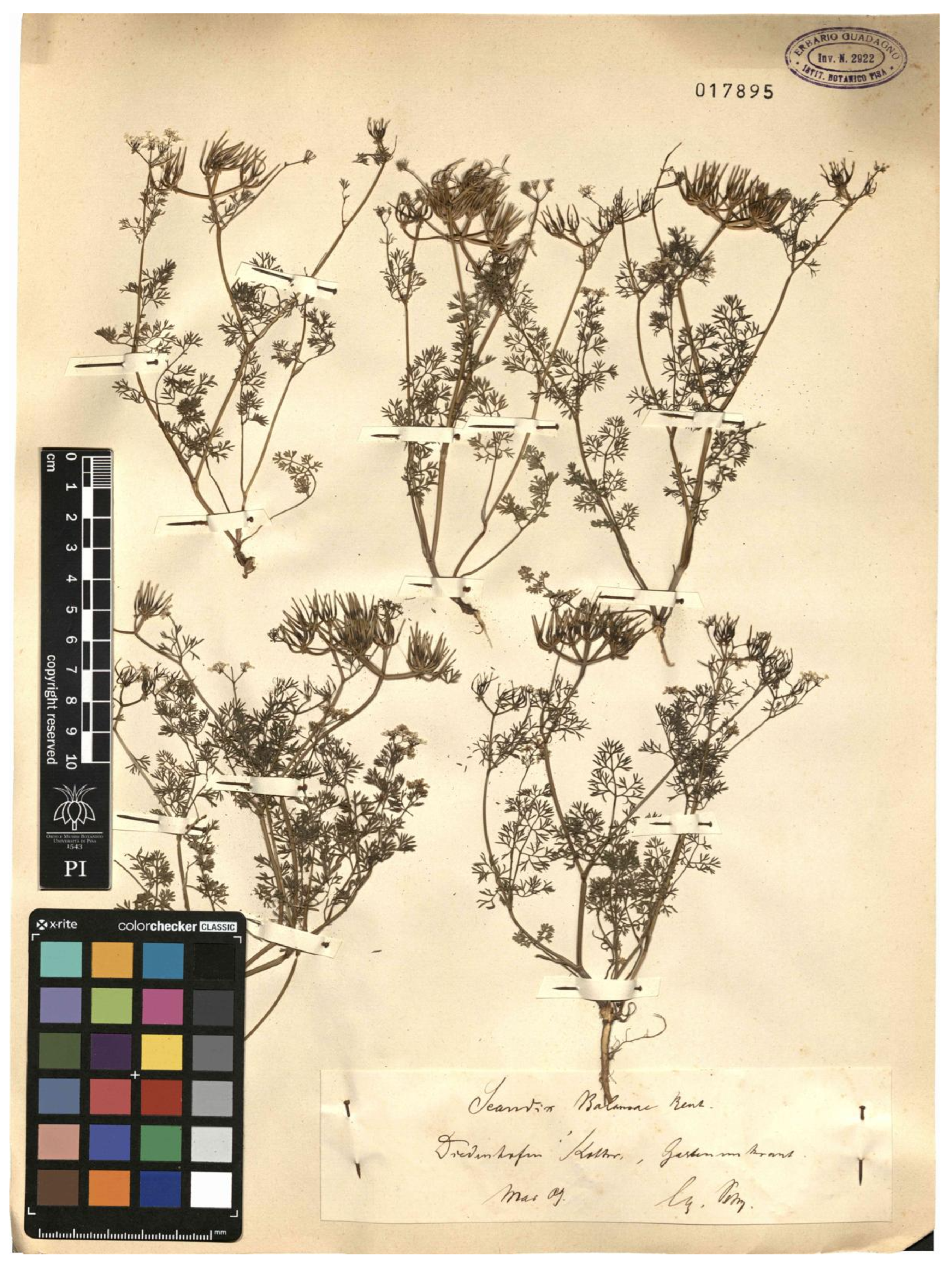
Figure A5.
Upper image, Table 7.
Figure A5.
Upper image, Table 7.
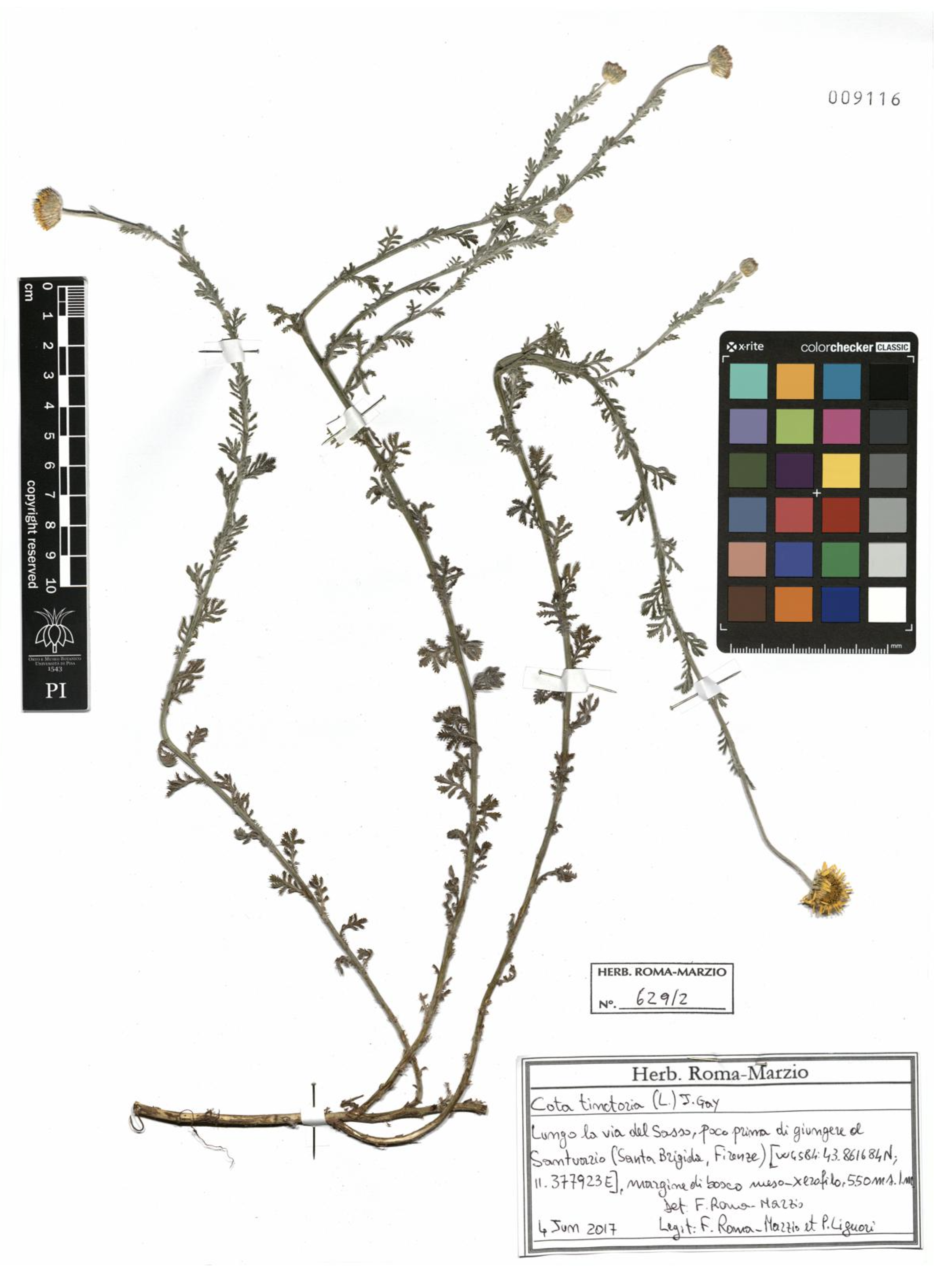
Figure A6.
Lower image, Table 7.
Figure A6.
Lower image, Table 7.
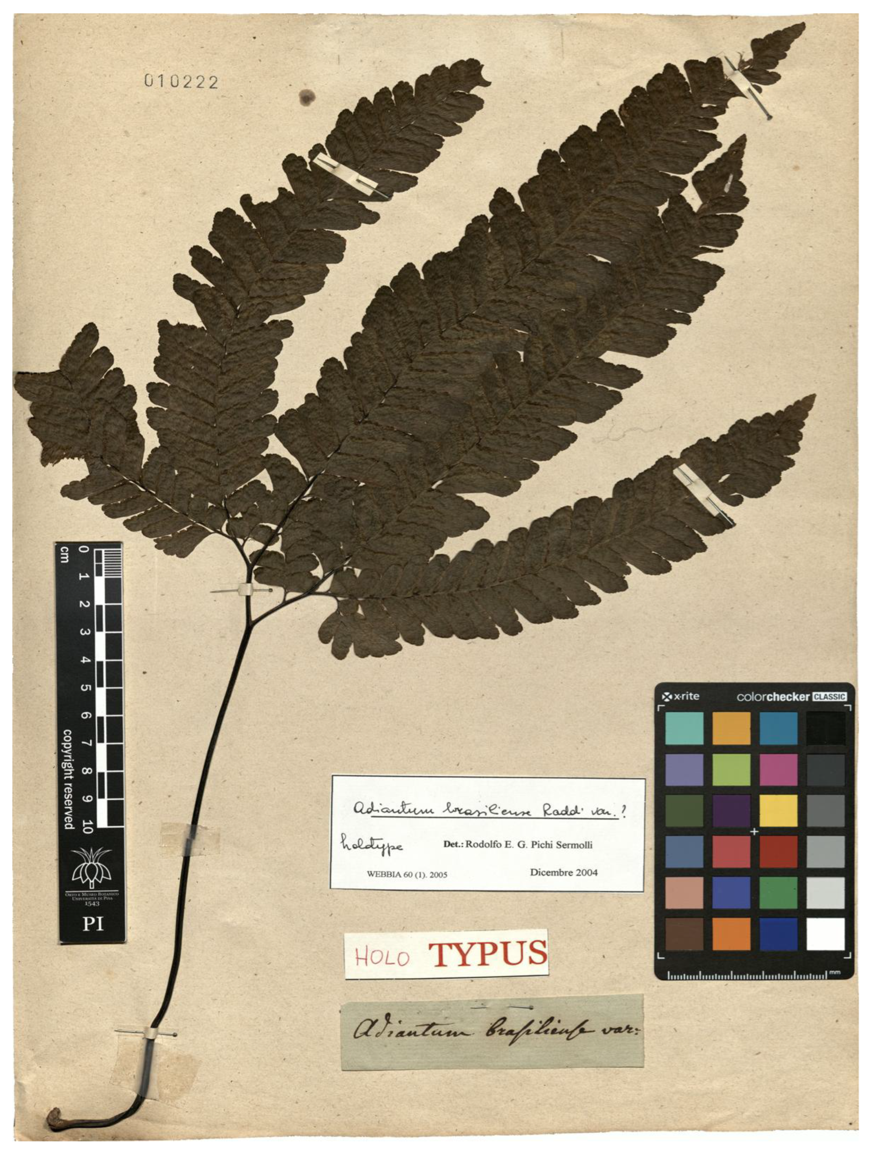
Figure A7.
Upper image, Table 8.
Figure A7.
Upper image, Table 8.
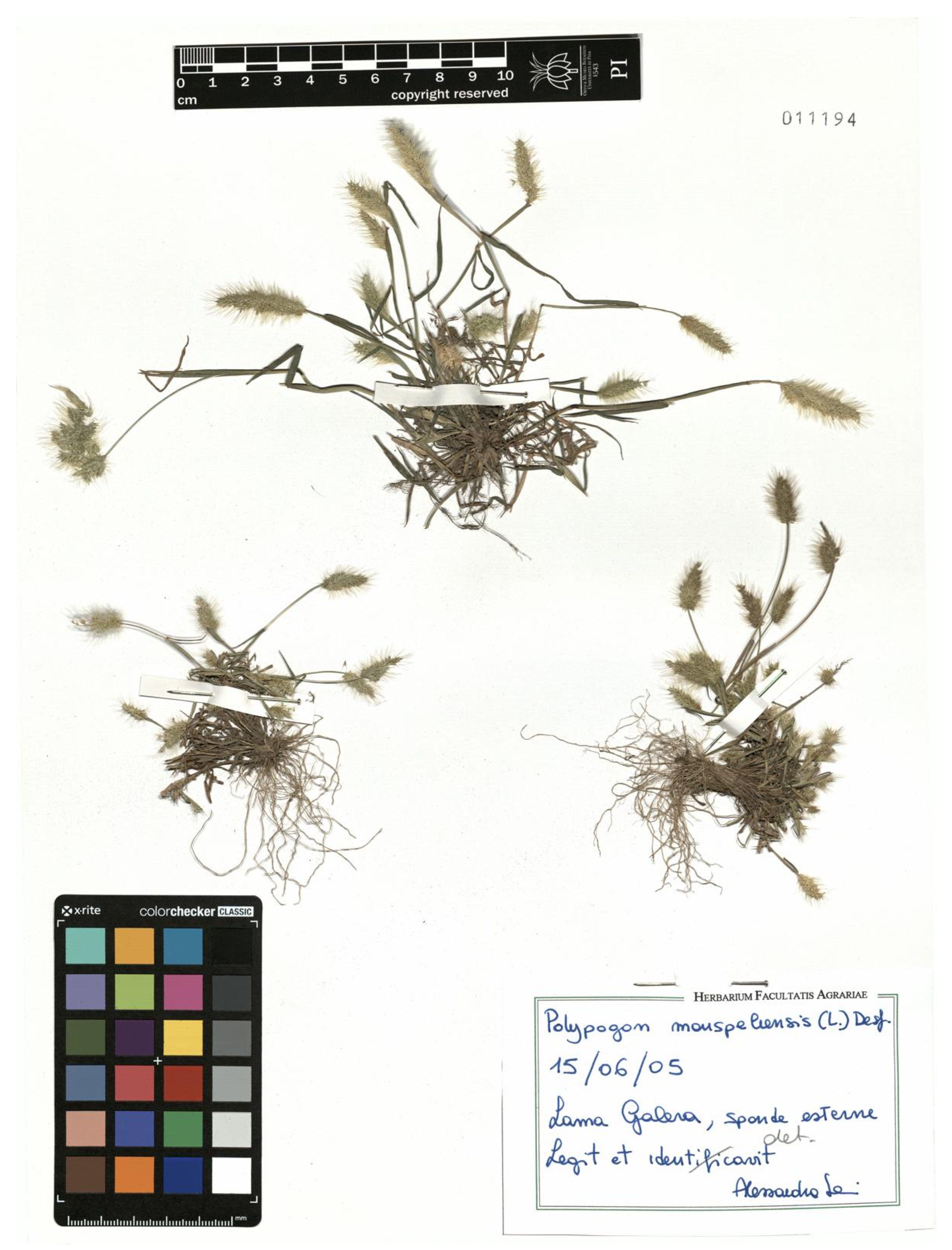
Figure A8.
Lower image, Table 8.
Figure A8.
Lower image, Table 8.
References
- Ariño, A.H. Approaches to Estimating the Universe of Natural History Collections Data. Biodivers. Informatics 2010, 7, 81–92. [Google Scholar] [CrossRef]
- Davis, C.C. The Herbarium of the Future. Trends Ecol. Evol. 2023, 38, 412–423. [Google Scholar] [CrossRef]
- Meineke, E.K.; Davies, T.J.; Daru, B.H.; Davis, C.C. Biological Collections for Understanding Biodiversity in the Anthropocene. Philos. Trans. R. Soc. B 2018, 374, 20170386. [Google Scholar] [CrossRef]
- Lane, M.A. Roles of Natural History Collections. Ann. Mo. Bot. Gard. 1996, 83, 536–545. [Google Scholar] [CrossRef]
- Lister, A.M. Natural History Collections as Sources of Long-Term Datasets. Trends Ecol. Evol. 2011, 26, 153–154. [Google Scholar] [CrossRef]
- Hedrick, B.P.; Heberling, J.M.; Meineke, E.K.; Turner, K.G.; Grassa, C.J.; Park, D.S.; Kennedy, J.; et al. Digitization and the Future of Natural History Collections. BioScience 2020, 70, 243–251. [Google Scholar] [CrossRef]
- Lendemer, J.; Thiers, B.; Monfils, A.K.; Zaspel, J.; Ellwood, E.R.; Bentley, A.; LeVan, K.; Bates, J.; Jennings, D.; Contreras, D.; et al. The Extended Specimen Network: A Strategy to Enhance US Biodiversity Collections, Promote Research and Education. BioScience 2020, 70, 23–30. [Google Scholar] [CrossRef] [PubMed]
- Hardisty, A.R.; Ellwood, E.R.; Nelson, G.; et al. Digital Extended Specimens: Enabling an Extensible Network of Biodiversity Data Records as Integrated Digital Objects on the Internet. BioScience 2022, 72, 978–987. [Google Scholar] [CrossRef]
- De Smedt, S.; Bogaerts, A.; De Meeter, N.; Dillen, M.; Engledow, H.; Van Wambeke, P.; Leliaert, F.; Groom, Q. Ten Lessons Learned from the Mass Digitisation of a Herbarium Collection. PhytoKeys 2024, 244, 23–37. [Google Scholar] [CrossRef]
- Nelson, G.; Ellis, S. The Impact of Digitization and Digital Data Mobilization on Biodiversity Research and Outreach. Biodiversity Information Science and Standards 2018, 2, e28470. [Google Scholar] [CrossRef]
- Martellos, S.; Zardini, M.; Seggi, L.; Conti, M.; Trabucco, R. Digitization of the Lichenotheca Veneta by Vittore Trevisan. Heritage 2024, 7, 7298–7308. [Google Scholar] [CrossRef]
- Mudge, M.; Malzbender, T.; Chalmers, A.; Scopigno, R.; Davis, J.; Wang, O.; et al. Image-Based Empirical Information Acquisition, Scientific Reliability, and Long-Term Digital Preservation. In Eurographics 2008 — Tutorials; Roussou, M., Leigh, J., Eds.; The Eurographics Association: Crete, Greece, 2008. [Google Scholar]
- Wieczorek, J.; Bloom, D.; Guralnick, R.; Blum, S.; Döring, M.; Giovanni, R.; Robertson, T.; Vieglais, D. Darwin Core: An Evolving Community-Developed Biodiversity Data Standard. PLoS One 2012, 7, e29715. [Google Scholar] [CrossRef]
- Sweeney, P.; Starly, B.; Morris, P.; Xu, Y.; Jones, A.; Radhakrishnan, S.; Grassa, C.; Davis, C. Large-Scale Digitization of Herbarium Specimens: Development and Usage of an Automated, High-Throughput Conveyor System. Taxon 2018, 67, 165–178. [Google Scholar] [CrossRef]
- Thiers, B.; Tulig, M.; Watson, K. Digitization of the New York Botanical Garden Herbarium. Brittonia 2016, 68, 324–333. [Google Scholar] [CrossRef]
- Barber, A.; Lafferty, D.; Landrum, L.R. The SALIX Method: A Semi-Automated Workflow for Herbarium Specimen Digitization. Taxon 2018, 62, 581–590. [Google Scholar] [CrossRef]
- Beaman, R.S.; Cellinese, N.; Heidorn, P.B.; Guo, Y.; Green, A.M.; Thiers, B. HERBIS: Integrating Digital Imaging and Label Data Capture for Herbaria. In Proceedings of the Botany 2006: Botanical Cyberinfrastructure, Chico, CA, USA, 15–19 July 2006. [Google Scholar]
- Granzow-de la Cerda, I.; Beach, J.H. Semi-Automated Workflows for Acquiring Specimen Data from Label Images in Herbarium Collections. Taxon 2010, 59, 1830–1842. [Google Scholar] [CrossRef]
- Heidorn, P.B.; Wei, Q. Automatic Metadata Extraction from Museum Specimen Labels. In Proceedings of the International Conference on Dublin Core and Metadata Applications, Berlin, Germany, 22–26 September 2008; pp. 57–68. [Google Scholar]
- Haston, E.; Cubey, R.; Pullan, M.; Atkins, H.; Harris, D. Developing Integrated Workflows for the Digitisation of Herbarium Specimens Using a Modular and Scalable Approach. ZooKeys 2012, 209, 93–102. [Google Scholar] [CrossRef]
- Johaadien, R.; Torma, M. "Publish First": A Rapid, GPT-4 Based Digitisation System for Small Institutes with Minimal Resources. BISS 2023, 7, e112428. [Google Scholar] [CrossRef]
- Alkamli, S.; Alabduljabbar, R. Understanding Privacy Concerns in ChatGPT: A Data-Driven Approach with LDA Topic Modeling. Heliyon 2024, 10, e39087. [Google Scholar] [CrossRef]
- Takano, A.; Cole, T.C.H.; Konagai, H. A Novel Automated Label Data Extraction and Database Generation System from Herbarium Specimen Images Using OCR and NER. Sci. Rep. 2024, 14, 112. [Google Scholar] [CrossRef]
- Vaswani, A.; Shazeer, N.; Parmar, N.; Uszkoreit, J.; Jones, L.; Gomez, A.N.; Kaiser, L.; Polosukhin, I. Attention Is All You Need. In Proceedings of the Advances in Neural Information Processing Systems, Long Beach, CA, USA, 4–9 December 2017; Volume 30. [Google Scholar] [CrossRef]
- Vilalta, R.; Giraud-Carrier, C.; Brazdil, P.; Soares, C. Inductive Transfer. In Encyclopedia of Machine Learning; Springer: Boston, MA, USA, 2011. [Google Scholar] [CrossRef]
- Tsai, Y.H.H.; Bai, S.; Liang, P.P.; Kolter, J.Z.; Morency, L.P.; Salakhutdinov, R. Multimodal Transformer for Unaligned Multimodal Language Sequences. In Proceedings of the 57th Annual Meeting of the Association for Computational Linguistics, Florence, Italy, 28 July–2 August 2019; pp. 6558–6569. [Google Scholar] [CrossRef]
- Li, M.; Lv, T.; Chen, J.; Cui, L.; Lu, Y.; Florencio, D.; Zhang, C.; Zhoujun, L.; Wei, F. TrOCR: Transformer-Based Optical Character Recognition with Pre-Trained Models. In Proceedings of the Thirty-Seventh AAAI Conference on Artificial Intelligence and Thirty-Fifth Conference on Innovative Applications of Artificial Intelligence and Thirteenth Symposium on Educational Advances in Artificial Intelligence, Washington, DC, USA, 7–14 February 2023; Volume 37, No. 11. pp. 13094–13102. [Google Scholar]
- Kim, G.; Hong, T.; Yim, M.; et al. OCR-Free Document Understanding Transformer. In Computer Vision–ECCV 2022; Lecture Notes in Computer Science; Springer: Cham, Switzerland, 2022; Volume 13688. [Google Scholar] [CrossRef]
- Bräuchler, C.; Schuster, T.M.; Vitek, E.; Rainer, H. The Department of Botany at the Natural History Museum Vienna (Herbarium W) – History, Status, and a Best Practice Guideline for Usage and Requests. Ann. Naturhist. Mus. Wien Ser. B 2021, 123, 297–322. [Google Scholar]
- Rainer, H.; Berger, A.; Schuster, T.M.; Walter, J.; Reich, D.; Zernig, K.; et al. Community Curation of Nomenclatural and Taxonomic Information in the Context of the Collection Management System JACQ. Biodiversity Information Science and Standards 2023, 7, e112571. [Google Scholar] [CrossRef]
- Roma-Marzio, F.; Maccioni, S.; Dolci, D.; Astuti, A.; Magrini, N.; Pierotti, F.; et al. Digitization of the Historical Herbarium of Michele Guadagno at Pisa (PI-GUAD). PhytoKeys 2023, 234, 107–125. [Google Scholar] [CrossRef] [PubMed]
- Park, S.; Shin, S.; Lee, B.; Lee, J.; Surh, J.; Seo, M.; Lee, H. CORD: A Consolidated Receipt Dataset for Post-OCR Parsing. In Proceedings of the Workshop on Document Intelligence at NeurIPS, Vancouver, BC, Canada, 14 December 2019. [Google Scholar]
- Hwang, A.; Frey, W.R.; McKeown, K. Towards Augmenting Lexical Resources for Slang and African American English. In Proceedings of the 7th Workshop on NLP for Similar Languages, Varieties and Dialects, Barcelona, Spain, 13 December 2020; pp. 160–172. [Google Scholar]
- Hong, T.; Kim, D.; Ji, M.; Hwang, W.; Nam, D.; Park, S. BROS: A Pre-trained Language Model Focusing on Text and Layout for Better Key Information Extraction from Documents. In Proceedings of the AAAI Conference on Artificial Intelligence, Philadelphia, PA, USA, 22 February–1 March 2022; Volume 36, No. 10. pp. 10767–10775. [Google Scholar]
- Xu, Y.; Li, M.; Cui, L.; Huang, S.; Wei, F.; Zhou, M. LayoutLM: Pre-Training of Text and Layout for Document Image Understanding. In Proceedings of the 26th ACM SIGKDD Conference on Knowledge Discovery and Data Mining, Virtual Event, CA, USA, 6–10 July 2020; pp. 1192–1200. [Google Scholar]
- Xu, Y.; Xu, Y.; Lv, T.; Cui, L.; Wei, F.; Wang, G.; Zhou, L. LayoutLMv2: Multi-Modal Pre-Training for Visually-Rich Document Understanding. In Proceedings of the 59th Annual Meeting of the Association for Computational Linguistics and the 11th International Joint Conference on Natural Language Processing, online, 1–6 August 2021; pp. 2579–2591. [Google Scholar]
- Yosinski, J.; Clune, J.; Bengio, Y.; Lipson, H. How Transferable Are Features in Deep Neural Networks? In Proceedings of the Advances in Neural Information Processing Systems, 2014, Vol. In Proceedings of the Advances in Neural Information Processing Systems, Montreal, QC, Canada, 8–13 December 2014; Volume 27. [Google Scholar] [CrossRef]
- Zhang, K.; Shasha, D. Simple Fast Algorithms for the Editing Distance Between Trees and Related Problems. SIAM J. Comput. 1989, 18, 1245–1262. [Google Scholar] [CrossRef]
- Lin, C.Y. ROUGE: A Package for Automatic Evaluation of Summaries. In Proceedings of the Text Summarization Branches Out, Barcelona, Spain, 25–26 July 2004; pp. 74–81. [Google Scholar]
- Zhong, X.; ShafieiBavani, E.; Jimeno Yepes, A. Image-Based Table Recognition: Data, Model, and Evaluation. In Computer Vision – ECCV 2020; Springer: Cham, Switzerland, 2020; Volume 12366. [Google Scholar] [CrossRef]
Figure 2.
Training loss curves of training from scratch (dotted lines) and fine-tuning (continuous line) with images at a resolution of 1200×1600. Training loss curves track the decrease in cross-entropy loss during training. Even with longer training if compared to fine-tuning, the training from scratch loss never decreases enough, evidencing a poorer performance.
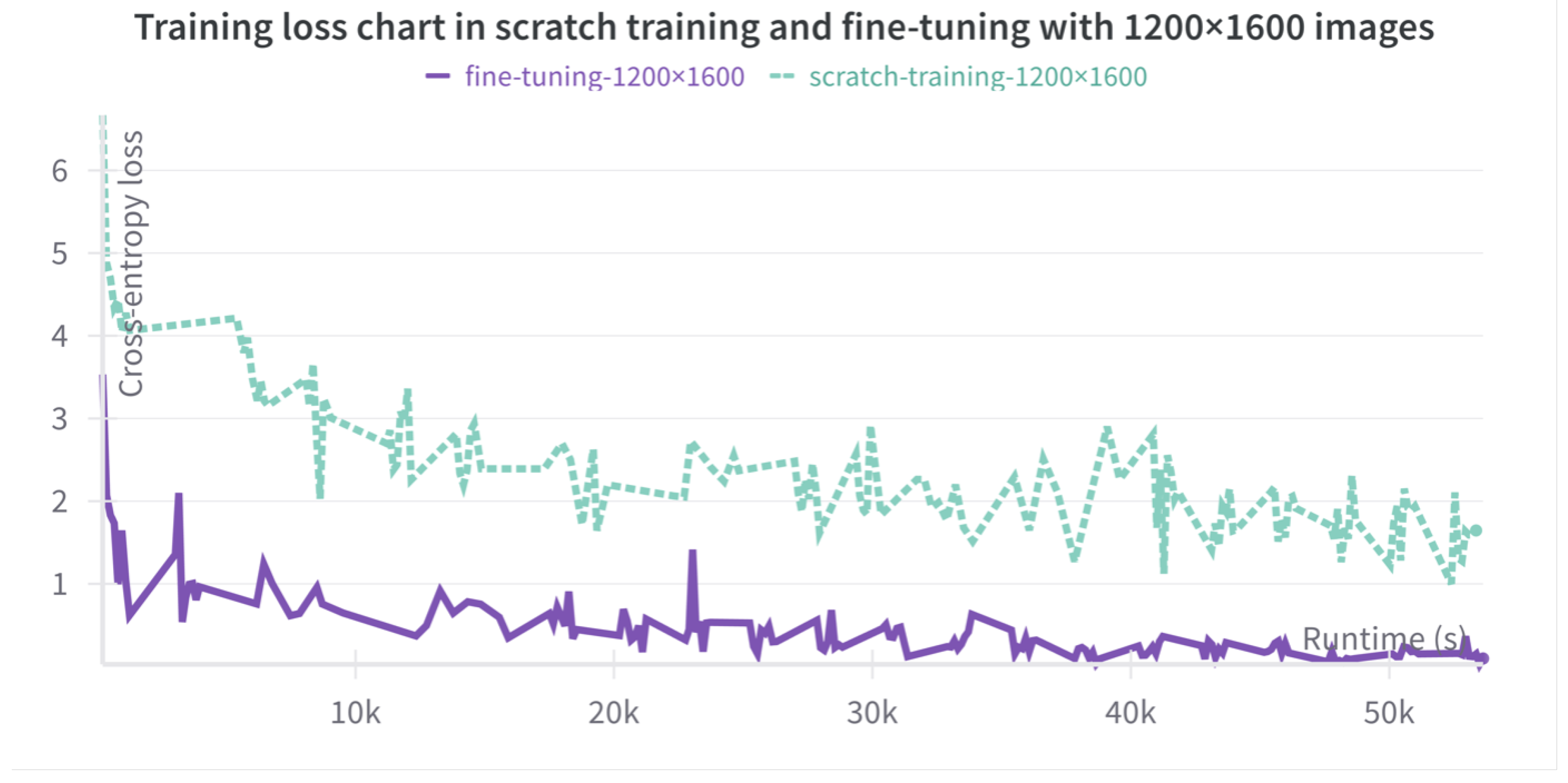
Figure 3.
Violin distribution chart of the evaluation on the test set of 1200×1600 images. The 25th and 75th percentiles respectively are 0.702 and 0.952. The median value and the average value have been reported in Table 3 and Table 4. More than 75% of test images achieved an accuracy score of more than 0.7. Test images with low accuracy scores are rare in the test set.
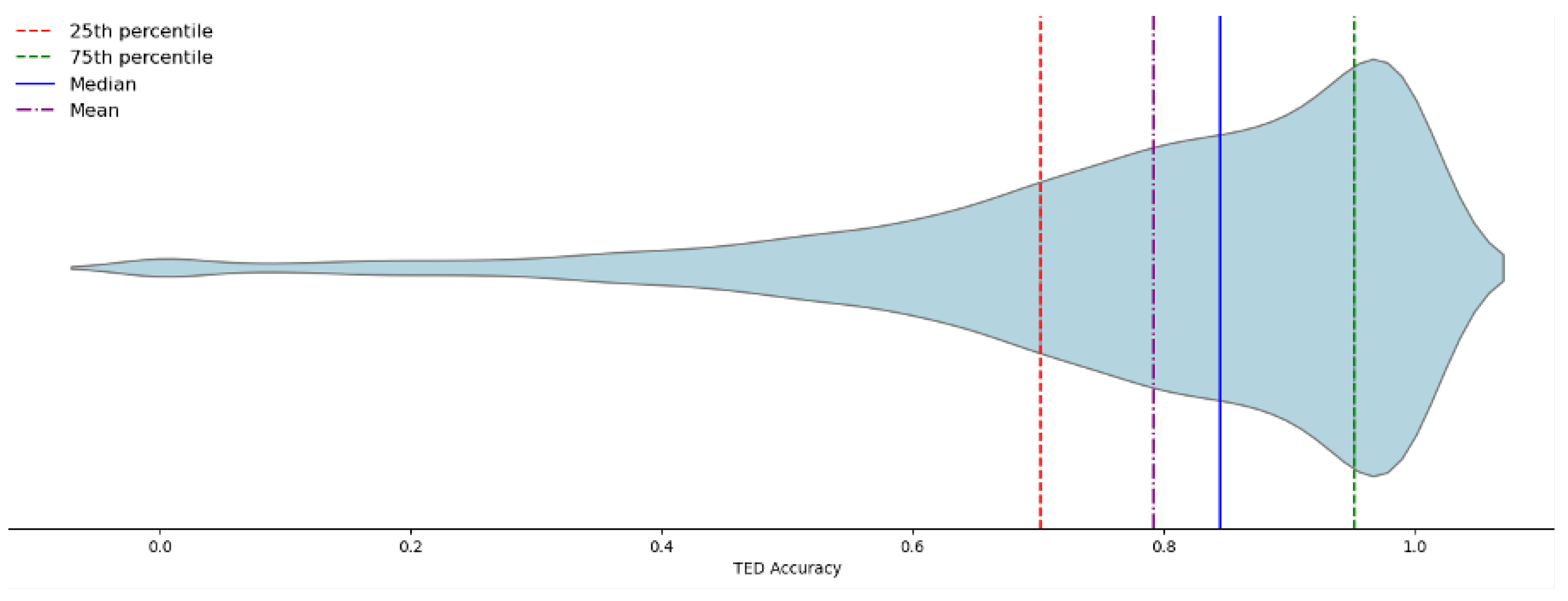

Table 1.
Comparison of the capabilities of different base models on the mainstream benchmark CORD dataset. Four features have been selected for the comparison of base models: (1) Text recognition, i.e., OCR shouldn’t be a bottleneck for text recognition; (2) Multi-lingual support, i.e., the base model should be able to deal with different languages; (3) Complex format support, i.e., the capability of accurate recognition in various document formats; (4) CORD score i.e., the Tree Edit Distance (TED) accuracy in CORD benchmark.
| (1) Text Recognition | (2)Multi-lingual Support | (3) Complex Format Support | (4) CORD Score (Tree-based edit distance Accuracy) [28] | |
|---|---|---|---|---|
| BERT [33] | External OCR | Yes | No | 65.5 |
| BROS [34] | OCR | No | No | 70.0 |
| LayoutLM [35] | OCR | No | Yes | 81.3 |
| LayoutLM v2 [36] | OCR | Yes | Yes | 82.4 |
| TrOCR [27] | OCR-free | No | No | NA |
| Donut [28] | OCR-free | Yes | Yes | 90.9 |
Table 2.
Batch size selected for three fine-tuning variations. The batch size is limited by the 64GB graphics memory and is correlated with the storage size of one image. Thus, the larger the resolution is, the smaller the batch size is.
Table 2.
Batch size selected for three fine-tuning variations. The batch size is limited by the 64GB graphics memory and is correlated with the storage size of one image. Thus, the larger the resolution is, the smaller the batch size is.
| 600×800 | 960×1280 | 1200×1600 | |
|---|---|---|---|
| Batch size | 10 | 8 | 5 |
Table 3.
Runtime and testing TED accuracy of three versions Donut fine-tuning with an image resolution of 600×800, 960×1280, and 1200×1600. Three variations were fine-tuned with the same Leonardo HPC system with four NVIDIA Ampere A100-64 GPUs to ensure the runtime was comparable among them. The test datasets used for testing TED accuracies of all fine-tuning versions are the same and kept apart from the training.
| Runtime (s) | Average Testing TED Accuracy | Median Testing TED Accuracy | Standard Deviation of Testing TED Accuracy | |
|---|---|---|---|---|
| 600×800 | 38,715 | 0.607 | 0.629 | 0.254 |
| 960×1280 | 59,027 | 0.750 | 0.806 | 0.227 |
| 1200×1600 | 55,119 | 0.788 | 0.851 | 0.218 |
Table 4.
Runtime and TED accuracies of training from scratch and fine-tuning with images at a resolution of 1200×1600. Both approaches (training from scratch and fine-tuning) used the same test dataset and hyperparameters for the evaluation.
Table 4.
Runtime and TED accuracies of training from scratch and fine-tuning with images at a resolution of 1200×1600. Both approaches (training from scratch and fine-tuning) used the same test dataset and hyperparameters for the evaluation.
| Runtime (s) | Validation TED accuracy | Average Testing TED accuracy | Median Testing TED accuracy | Standard deviation of testing TED accuracy | |
|---|---|---|---|---|---|
| Scratch Training | 54,729 | 0.697 | 0.181 | 0.202 | 0.110 |
| Fine-tuning | 55,119 | 0.929 | 0.788 | 0.851 | 0.218 |
Table 5.
Recognition examples with zero scores from the fine-tuned model with 1200×1600 images. Complex labels containing a lot of additional information, biased ground truth, and images containing more than one specimen produce the worst TED accuracy scores. However, these scores could sometimes be interpreted as “false negatives” (see text). In red, in which the ground truth and the prediction differ; in green, in which both match.
| Specimen (Figure A1, Figure A2) | Ground truth | Recognition | Accuracy score |
|---|---|---|---|
 |
 |
 |
0 |
 |
 |
 |
0 |
Table 6.
Recognition examples with low scores from the fine-tuned model with 1200×1600 images. Images containing more than one label and untidy handwriting can produce poor TED accuracy scores. In red, in which the ground truth and the prediction differ; in green, in which both match.
Table 6.
Recognition examples with low scores from the fine-tuned model with 1200×1600 images. Images containing more than one label and untidy handwriting can produce poor TED accuracy scores. In red, in which the ground truth and the prediction differ; in green, in which both match.
| Specimen (Figure A3, Figure A4) | Ground truth | Recognition | Accuracy score |
|---|---|---|---|
 |
 |
 |
0.204 |
 |
 |
 |
0.231 |
Table 7.
Recognition examples with high scores from the fine-tuned model with 1200×1600 images. Labels containing minor additional information or special characters, and images containing tidy handwritings, normally result in quite good results in TED accuracy scores. In red, in which the ground truth and the prediction differ; in green, in which both match.
| Specimen (Figure A5, Figure A6) | Ground truth | Recognition | Accuracy score |
|---|---|---|---|
 |
 |
 |
0.899 |
 |
 |
 |
0.844 |
Table 8.
Recognition examples with full scores from the fine-tuned model with 1200×1600 images. Specimen sheets with one label alone, hosting little to no additional information and very clean handwriting (or typewritten), normally result in very high TED accuracy scores. In red, in which the ground truth and the prediction differ; in green, in which both match.
| Specimen (Figure A7, Figure A8) | Ground truth | Recognition | Accuracy score |
|---|---|---|---|
 |
 |
 |
1.0 |
 |
 |
 |
1.0 |
Disclaimer/Publisher’s Note: The statements, opinions and data contained in all publications are solely those of the individual author(s) and contributor(s) and not of MDPI and/or the editor(s). MDPI and/or the editor(s) disclaim responsibility for any injury to people or property resulting from any ideas, methods, instructions or products referred to in the content. |
© 2025 by the authors. Licensee MDPI, Basel, Switzerland. This article is an open access article distributed under the terms and conditions of the Creative Commons Attribution (CC BY) license (http://creativecommons.org/licenses/by/4.0/).
Copyright: This open access article is published under a Creative Commons CC BY 4.0 license, which permit the free download, distribution, and reuse, provided that the author and preprint are cited in any reuse.


