Submitted:
26 November 2025
Posted:
02 December 2025
You are already at the latest version
Abstract
Based on the Muskat-Leverett two-phase filtration equations, a model problem of water and air movement in melting snow is considered, taking into account the external heat flow. The maximum principle and the finite-velocity lemma for perturbations are proven for water saturation. An algorithm for numerically studying the self-similar problem is presented. Calculations of the temperature and water saturation distributions by depth are presented. The significant influence of the specified flux at the boundary and the thermal conductivity coefficient on the temperature field in the snow layer is demonstrated, which is important for predicting melting and hydrothermal processes in snow and ice covers. A theorem on the existence of a weak solution to this problem is formulated. A literature review is provided on mathematical models of multiphase filtration in porous media, taking into account phase transitions (melting, sublimation) and external heat fluxes.
Keywords:
snow
; melting
; heat flow
; inhomogeneous medium
; phase transitions
; multiphase filtration
; porous medium
1. Introduction
Recently, various snow cover models have become increasingly popular. They are used to solve problems related to avalanche movement, the contribution of snow cover to runoff formation in river basins, and the spread of pollutants in melting snow. The thermal balance and regime of the earth’s surface are shaped by a powerful natural factor—solar radiation flux. Accounting for solar radiation flux is important during snowmelt, as it allows for more accurate predictions of the thermal regime of the snow-ice cover and the thermodynamic processes within it. Models typically use surface temperature as a boundary condition, which ignores important physical processes occurring in the uppermost layer of snow. Solar radiation flux significantly influences the thermal balance of the snow and ice surface, where intense processes such as melting, evaporation, and other processes occur in the near-surface layer under the influence of radiation, exerting a decisive influence on the dynamics of the underlying snow cover and the thermal regime. Snow and ice are light-scattering media over a fairly wide range of the solar radiation spectrum, so their optical properties must be taken into account.
One way to account for heat flux in snowmelt modeling is to specify it for the boundary layer on the snow surface. This method for determining heat flux is presented in the work [1], where a condition for heat exchange with the atmosphere was specified at the upper boundary of the soil (or snow cover), while a geothermal heat flux was introduced at the lower boundary. The boundary condition at the snow-soil boundary determined the equality of temperatures and heat fluxes. The work included calculations to assess the influence of various factors on the snow surface temperature and the development of a method for determining the thermal stability of the snow cover and the effective thermal conductivity of snow based on the temperature of the upper soil layer.
Another method is the partial reflection of shortwave radiation from the snow surface and its partial penetration into the snow layer. In many studies, this process is presented in the form of Bouguer’s law [2], which takes into account such important optical properties as the scattering coefficient, the attenuation coefficient, and albedo. The albedo for snow, where the attenuation coefficient reaches 30–60 m−1, reaches limit values close to 100 [2]. Thus, freshly fallen snow is characterized by the highest albedo value A>90[2]. A good description of the reflectivity of snow cover is presented in the work [3], which also proposes a model for calculating the albedo based on air temperature and total solar radiation data, which can be used in the absence of observations. In [4], a one-dimensional multiphase model of snow cover was considered, in which the change in heat content for each phase is described by a heat flux equation accounting for convection, thermal conductivity, solar radiation, and phase transitions.
The heat flux in [5] to describe heat and moisture exchange in snow was defined based on P.P. Kuzmin’s method. The flux accounted for direct and diffuse shortwave radiation, longwave radiation from the atmosphere, longwave radiation from snow, turbulent heat exchange, heat exchange during evaporation, and heat input with liquid precipitation. To model the hydrothermal regime of snow cover at subzero temperatures, a heat source was used due to the absorption of shortwave radiation flux within the snowpack, based on the Bouguer-Lambert law. Problems of heat and mass transfer in melting snow and ice cover without taking into account an external heat source were considered in works [6,7,8,9,10,11].
In the paper [12], a heat and moisture exchange model was developed that calculates all components of the heat and water balance on land, as well as state variables (effective landscape surface temperature, soil temperature, soil moisture content, amount of frozen water in the soil, albedo, etc.). Here, the transfer of shortwave radiation within the snowpack is taken into account in the temperature equation, the radiation intensity varies with depth according to the Bouguer-Lambert law, and an empirical relationship is proposed for determining the attenuation coefficient. For the albedo coefficient, the relationship from [13] was used, taking into account the aging of the upper snow layer.
The process of radiative snowmelt is described in detail in the paper [14]. Experimental studies were conducted to examine the influence of the radiation component on the snowmelt process and changes in snow cover albedo. The paper [15] compares two parameterizations for solar radiation transfer in sea ice. The first assumed exponential radiation decay with constant transmittance and attenuation coefficients. The second employed a two-layer scheme for solar radiation penetration into ice, simulating the near-surface transition layer. Numerical experiments were conducted to simulate the seasonal evolution of the snow-ice cover thickness and the vertical temperature profile within it.
2. Statement of the Problem
Melting snow is considered as a three-phase medium consisting of water (), air (), and ice (). The process is described using the mass conservation equation for each phase, the generalized Darcy law, and the energy conservation equation for melting snow [5,16,17,18]:
Here t is the time; is the velocity of the i-th phase; - the reduced density related to the true density and the volume concentration by the relation (the condition is a consequence of the definition of ); is the intensity of the transition of mass from the j-th to the i-th component in unit volume per unit time; are the filtration rates of water and air; is the porosity of snow; , – water and air saturation (, , ); – permeability tensor, – relative phase permeabilities (), – dynamic viscosity, – phase pressures, – capillary pressure , is the gravity acceleration vector; – temperature of the environment (, ); – heat capacity of the i -th phase at constant volume; – specific heat of fusion of ice; – thermal conductivity of snow (, , , [5]).
3. Self-Similar Solution to the Problem
We introduce the final values of temperature , and (ice melting point). Let . We assume that for all the following relations hold: when , when , for . Here, , are the given parameters. In addition, it is assumed that the porous medium is homogeneous (); (these conditions do not affect the generality of the results), in the coordinate system the vector , the functions included in the system (1) - (3) depend on . Eliminating in (1) , we obtain the system of equations
For the system (4) - (7) consider the following problem: snow occupies the area of , . At , there is no water (, ), the air is stationary () and the temperature is set to (below the melting point ice); at the velocities of water and air are known (, ), the air pressure is () and the boundary condition is set ( is the heat transfer coefficient, is the atmospheric air temperature, Q is the set heat flow). Assuming that all the sought functions depend only on the variable (c is an unknown constant) from (4) - (7) we obtain
The sought functions are , , , and the constant c. The solution to problem (8) - (13) is constructed as follows. We find the constant c and obtain representations for the filtration rates and temperature by integrating equations (8), (9) and (10). Using these representations and (10), we arrive at an equation for the saturation of . Investigation of the solvability of the problem for completes the construction of the solution to the problem (8)-(13). In the following, we use the notation .
Definition 1. A weak solution to the problem (8)–(13) is the function , , , and a fixed parameter c if:
- 1) the function has a continuous derivative and satisfies the equationand the conditions , , ;
- 2) the function has a continuous derivative with weight (), which satisfies the equationand the conditions , ;
- 3) the functions satisfy the equalitiesand the conditions , ;
- 4) the functions satisfy the equalitiesand the condition .
Determination of filtration rates
Representation for Temperature
Considering (14), (15) under the conditions (13), for unknown parameters c, , (, ), we obtain the following nonlinear system of equations
From the equation for temperature: then the system can be rewritten as:
here
For from (21) we obtain
Here , , , .
For from (21) we obtain
Here The solvability of this problem is proved in detail in [6]. Thus, for a given function , the representation (21) and its special cases (22), (23) determine the temperature for all .
The system solution for unknown parameters , , is divided into three stages:
1. Let , then , and .
To find , we consider the options and use the flow condition on the boundary.
If , then , - the solution is nonphysical.
If , then and - the solution is nonphysical.
For the case , we substitute c into and get:
This is the quadratic equation for :
where
,
,
. Here are given parameters, and the parameters must be subject to conditions so that the following relations are satisfied:
- If , then there are no real roots.
- If and , then there are no solutions.
-
If and , then the solution is:here must satisfy the condition .
-
If , then there are two roots:, which
- –
- for must satisfy the condition ;
- –
-
for must satisfy the inequalitiesand .
, which- –
- for is not a solution;
- –
-
for must satisfy the inequalitiesand .
2. Let , then , .
To find , we consider the options and use the flow condition on the boundary.
If , then , - the solution is nonphysical.
If , then and - the solution is nonphysical.
For the case , we substitute c into and get:
This is the quadratic equation for :
where
,
,
.
Here are given parameters, and the parameters must be subject to conditions so that the following relations are satisfied:
- If , then there are no real roots.
- If and , then there are no solutions.
-
If and , then the solution is:here must satisfy the condition .
-
If , then there are two roots:, which
- –
- for must satisfy the condition ;
- –
-
for must satisfy the inequalitiesand .
, which- –
- for is not a solution;
- –
-
for must satisfy the inequalitiesand .
3. Let and , then , .
To find , we consider the options and use the flow condition on the boundary.
If , then , - the solution is nonphysical.
If , then and - the solution is nonphysical.
For the case , we substitute c into and get:
This is the quadratic equation for :
where
,
,
.
Here are given parameters, and the parameters must be subject to conditions so that the following relations are satisfied:
- If , then there are no real roots.
- If and , then there are no solutions.
-
If and , then there is a solution:where must satisfy the condition .
-
If , then there are two roots:, which
- –
- for must satisfy the condition ;
- –
-
for must satisfy the inequalitiesand .
, which- –
- for is not a solution;
- –
-
for must satisfy the inequalitiesand .
Determination of saturation and pressure
From (10) and (16) we have
Eliminating and from these relations using the second equation in (10), we obtain
Following [6], we set: , . For , the relative phase permeabilities are defined as follows: for , for , for . Here we have the constants .
The function for and for and is assumed. Using the equation for temperature (17), we represent the equation for saturation in the form
where for , for , for ,
Equation (24) is considered for and the condition , that is, for the Cauchy problem is considered, and the condition must be justified.
To find the pressures and , we consider the equality following from Darcy’s laws (the first equations in (10))
If the functions and are found, then the filtration rates and pressures are determined by formulas (16), (26).
Let us assume that the functions , , , , satisfies the following conditions ():
Theorem 1.
The function is monotone in and , . There exists a point such that for all .
Consider the problem
The solvability of this problem is proved in detail in [6].
Let , . For , instead of (27), we consider the problem
Lemma 1. If is a solution problem (28) and , then .
Proof of Lemma 1.
The function is continuous on the interval and, therefore, there exists a value . Therefore, we can consider the problem
where
Lemma 2. Let be a solution to problem (29) and let the condition , be satisfied. Then there exists a point such that for all . If and additionally , then .
Proof of Lemma 2.
From (29) it follows
Here
We have
where , , . Using the representation (26) for , we obtain
where
Integrating equation (30) over from an arbitrary value to , we obtain
Here with and for . The last integral converges by the assumptions of Lemma 2, so for all , where satisfies the condition
Then it follows from the definition of that for . Let , (in this case satisfies the first equation in (29)). If is a solution of (29), then, by Lemma 1, the functions are continuous in . Let us consider a small neighborhood of the point , assuming that at the point , the inequality holds. For from equation (30) we obtain
by choosing accordingly. Then , i.e. and, therefore, . Repeating this process, at the k -th step we obtain , , . When k reaches a value for which the inequality is satisfied, using (31), we obtain , . The lemma is proved. □
4. Numerical Investigation
In the one-dimensional self-similar case, the system (1-3) is written in the form (8-13). Equations (7) for and (24) for s, which will be calculated numerically, will take the form:
Since the coefficient can turn to zero, then when dividing by it, is added and is taken.
Algorithm for numerical solution of self-similar problem
Let us introduce a grid , , h — step along the spatial coordinate.
We approximate the Newton’s boundary condition:
Equation (32) is approximated by an implicit Runge-Kutta scheme of fourth order accuracy [20]
where , , ,
.
From here
To find the nonlinear equations (32-33) were solved by successive approximations with an inner cycle over k:
1) assuming for the first approximation, was taken equal to , then was found from (36);
2) in the next iteration , was substituted into (34), where was found from the boundary condition;
3) steps 1-2 are repeated until the conditions and , where , are satisfied.
The velocity c is substituted in the equation for the temperature (32), which is considered to be the Runge-Kutta method of the 4th order of accuracy.
The numerical algorithm for the temperature equation was verified by computational experiments. To simplify the calculations, was taken as a trial temperature function. An exact solution for this equation was analytically found. Runge’s rule was applied: three calculations were performed on grids with steps , , .
The equation for water saturation (33) is also approximated by an implicit Runge-Kutta scheme of fourth order accuracy
where , , ,
.
is calculated using the formula , taking into account the found .
Figure 1 shows the results of the numerical modeling of temperature and water saturation with depth for the following parameters: , , , , , , , , , . The graph of the porosity function is shown in Figure 2.
Figure 3 shows the effect of a given heat flux Q on the temperature at the boundary. It is evident that with increasing Q, the temperature of the upper snow layer also increases. Water saturation remains unchanged.
The results of modeling temperature variations with depth as a function of thermal conductivity are presented in Figure 4. The graph shows that thermal conductivity directly influences snow heating: the higher the value of , the more intense the snow heating. Minor changes in water saturation are observed.
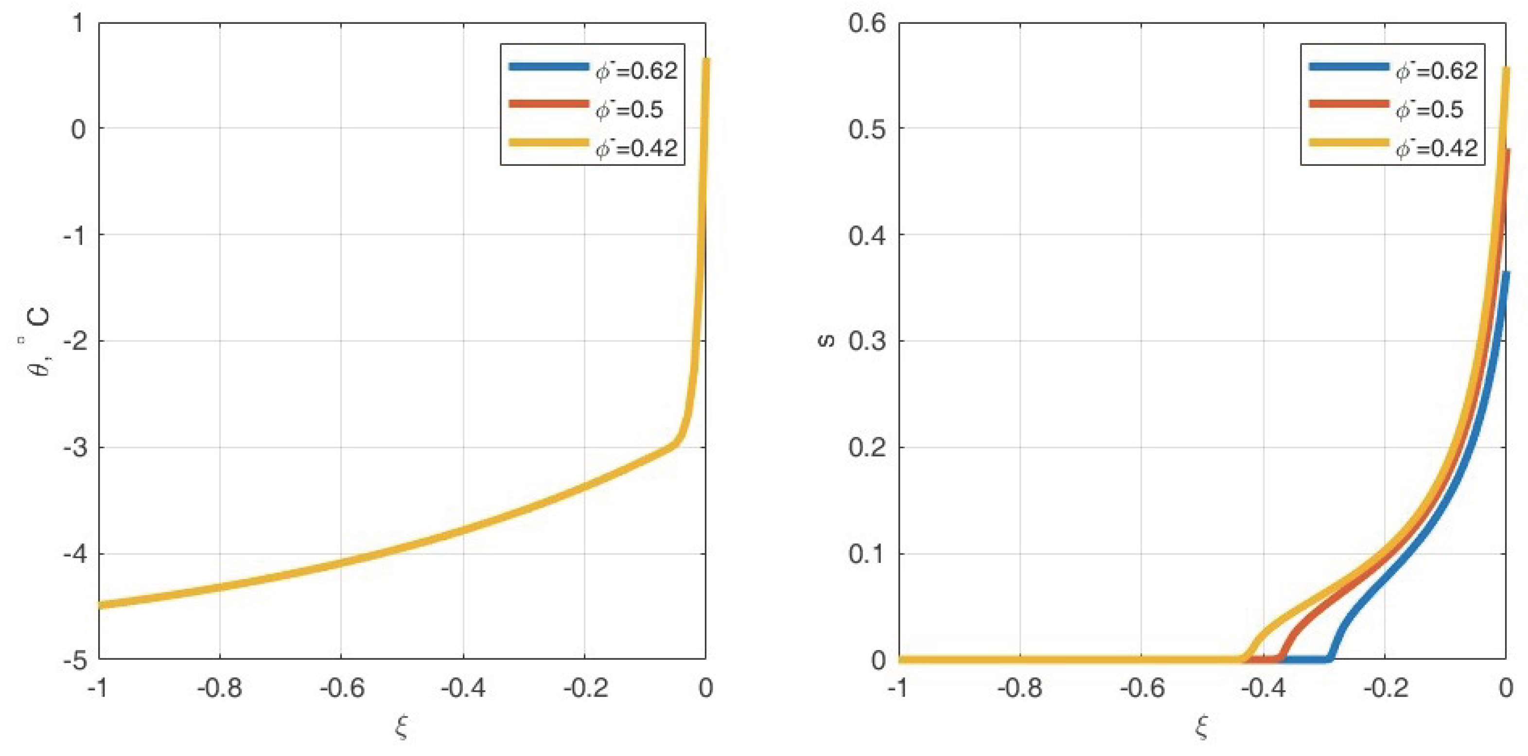
The specified porosity influences water saturation at the boundary (Figure 5), as is evident from the formula for . The calculations were performed with the specified parameters , , and three different values of . The temperature remains unchanged.
5. Conclusions
An exact self-similar solution to the problem of heat and mass transfer in snow and ice cover is constructed, taking into account variable porosity and phase transitions. The solution takes into account the influence of solar radiation flux at the boundary. For water saturation, the maximum principle and the lemma on the finite propagation velocity of disturbances are proven. A theorem on the existence of a weak solution to the problem is formulated. A numerical study of the problem of heat and mass transfer in snow is conducted, taking into account the external heat flux. The results of numerical modeling of temperature and water saturation are presented. The influence of a given heat flux at the boundary and the thermal conductivity coefficient on the temperature distribution over depth is demonstrated. The program is written in C++.
The work was carried out in accordance with the State Assignment of the Russian Ministry of Science and Higher Education entitled ‘Modern models of hydrodynamics for environmental management, industrial systems and polar mechanics’ (Govt. contract code: FZMW-2024-0003).
Appendix A

Table A1.
Parameter values.
| Parameter | Value |
|---|---|
| true density of water, | 1000 [] |
| true density of air, | 1.2928 [] |
| true density of ice, | 925 [] |
| heat capacity of water at constant pressure, | 4187 [] |
| heat capacity of air at constant pressure, | 1005 [] |
| heat capacity of ice at constant pressure, | [] |
| specific heat of melting of ice, | 335000 [] |
| boundary value of temperature, | 268.15 [K] |
| freezing point of water, | 270.15 [K] |
| melting point of ice, | 273.15 [K] |
| water filtration rate, | |
| air filtration rate, | |
| air pressure, | 1.0332 [kg/ms2] |
| filtration tensor, | 10−9[m2] |
| dynamic viscosity coefficient of water, | 0.17865 [kg/ms] |
| relative phase permeability of water, | 1 |
| relative phase permeability of air, | 1 |
| acceleration vector of gravity, | 9.8 [m/s2] |
| snow porosity at temperature , | 0.62 |
| snow porosity at temperature , | |
| snow porosity, | |
| thermal conductivity of snow, | [kg m/s3 K] |
| snow density, | +30 (1-) |
| reduced relative phase permeability of water, | |
| reduced relative phase permeability of air, |
References
- Kotlyakov V. M., Sosnovsky A. V. Evaluating the Thermal Resistance of Snow Cover by Ground Temperature// Water Resources — 2021. — Vol. 61, No. 2, P. 195 — 205. [CrossRef]
- Krass M. S., Merzlikin V. G. Radiation thermophysics of snow and ice — Leningrad: Gidrometeoizdat. 1990. — p. 261. [in Russian].
- Trofimova E. B. Reflectivity of snow cover // Proceedings of the All-Russian scientific and methodological conference—2014— pp. 1498 — 1500. [in Russian].
- Trofimova E. B. Reflectivity of snow cover. // Proc. IV All-Union Hydrological Congress. (USSR, M.)— 1976 — Vol 6. [in Russian].
- Kuchment, L. S. Formation of River Runoff. Physico-Mathematical Models. M. — 1983.
- Papin A. A. Solvability of the model problem of heat and mass transfer in melting snow // Journal of Applied Mechanics and Technical Physics. 2008. Vol. 49. No. 4. pp. 13-23. [CrossRef]
- Papin A.A. Boundary value problems of two-phase filtration // Publishing house of Altai State University. Barnaul, 2009, p. 220. [in Russian].
- Korobkin A.A., Papin A.A., Khabakhpasheva T.I. Mathematical models of snow and ice cover. Altai State University Publishing House, 2013. ISBN 978-5-7904-1515-6 [in Russian].
- Sibin A. N., Papin A. A. Heat and mass transfer in melting snow // Journal of Applied Mechanics and Technical Physics. 2021. Vol. 62. No. 1. P. 96-104. [CrossRef]
- Sibin A. N., Papin A. A. Modeling the movement of dissolved salt in melting snow // Journal of Applied Mechanics and Technical Physics. – 2024. – Vol. 65, No. 1. – P. 50-60. [CrossRef]
- Sibin A.N., Papin A.A. Mathematical modeling of filtration in media with variable porosity: monograph. – Barnaul: Publishing house of Altai State University, 2022. – 115 p. ISBN 978-5-7904-2591-2 [in Russian].
- Shmakin A. B., Turkov D. V., Mikhailov A. Yu. Model of snow cover with inclusion of layered structure and its seasonal evolution // Earth’s Cryosphere. — 2009 — Vol. 13, No. 4. — pp. 69 — 79. [in Russian]. in Russian.
- Dickinson R. E., Williamson D., Henderson-Sellers A. Biosphere–atmosphere transfer scheme (BATS) for the NCAR community climate model. —Boulder, Colorado. 1986. — P. 69.
- Gritsuk I. I., Debolskiy V. K., Maslikova O. Ya., Ponomarev N. K., Sinichenko E. K. Experimental study of the influence of solar radiation on the intensity of snow melting // Bulletin of RUDN, series Engineering research. — 2015. — No. 1. — p. 83 — 90.
- Zavyalov D. D., Solomakha T. A. Parameterization of solar radiation absorption by snow-ice cover in a thermodynamic model of the Azov Sea ice // Marine Hydrophysical Journal. —2021 — Vol. 37, No. 5. — p. 538 — 553. [CrossRef]
- Daanen, R. P., Nieber J. L. Model for coupled liquid water flow and heat transport with phase change in a snowpack // Journal of Cold Regions Engineering. — 2009. — Vol. 23, No. 2. — P. 43–68. [CrossRef]
- Tokareva M. A., Papin A. A. Boundary Value Problems for Filtration Equations in Poroelastic Media — Barnaul: Altai University Press, 2020. — P. 142.
- Papin A. A., Tokareva M. A. Problems of heat and mass transfer in the snow-ice cover // Polar Mechanics 2018. IOP Conf. Series: Earth and Environmental Science. — 2018. — Vol. 193. — P. 1–8. [CrossRef]
- Hartman F. Ordinary differential equations. — M.: MIR, 1970. [in Russian].
- Samarsky A. A., Gulin A. V. Numerical methods // Moscow: Nauka. Ed. in chief of physical and mathematical literature, 1989. — 432 p. [in Russian].
Figure 1.
Change in temperature and water saturation
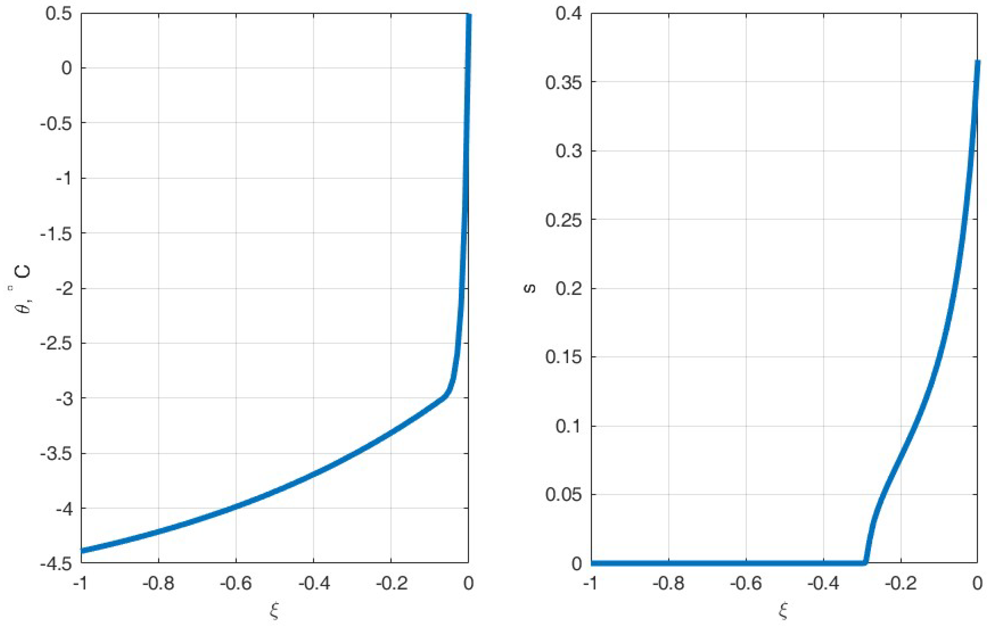
Figure 2.
Change in porosity.
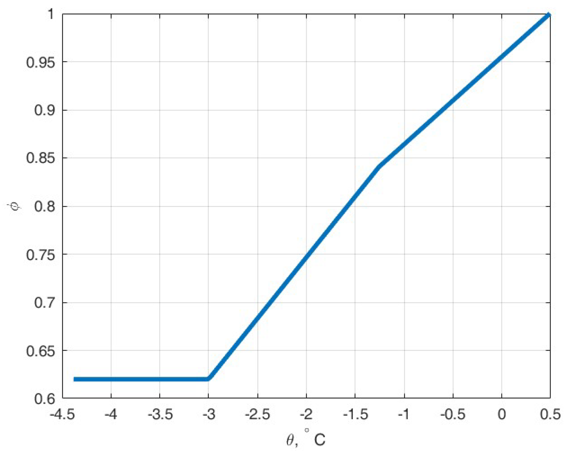
Figure 3.
Effect of heat flux Q on boundary temperature at , , , .
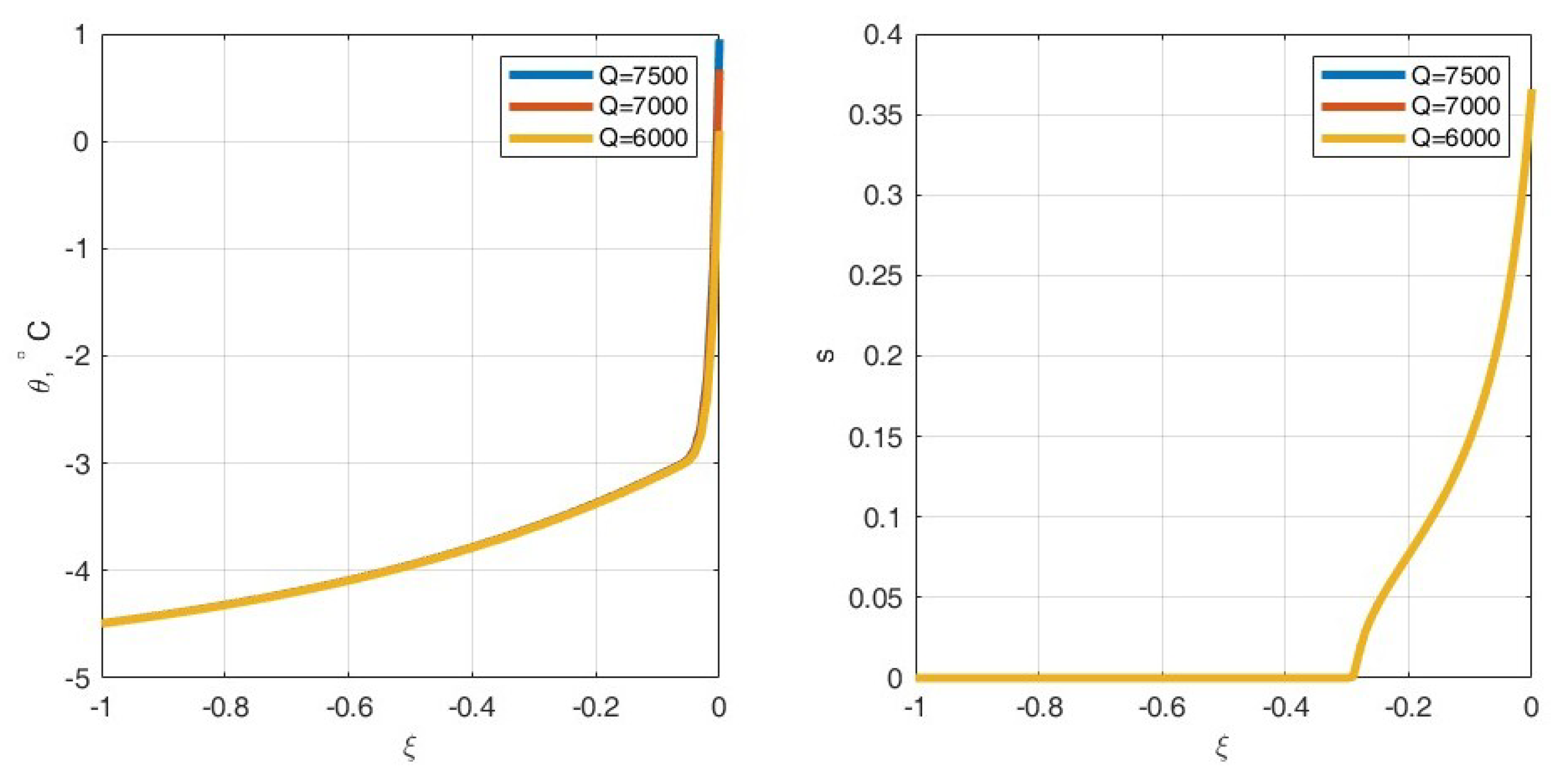
Figure 4.
Effect of thermal conductivity coefficient on temperature at , ,
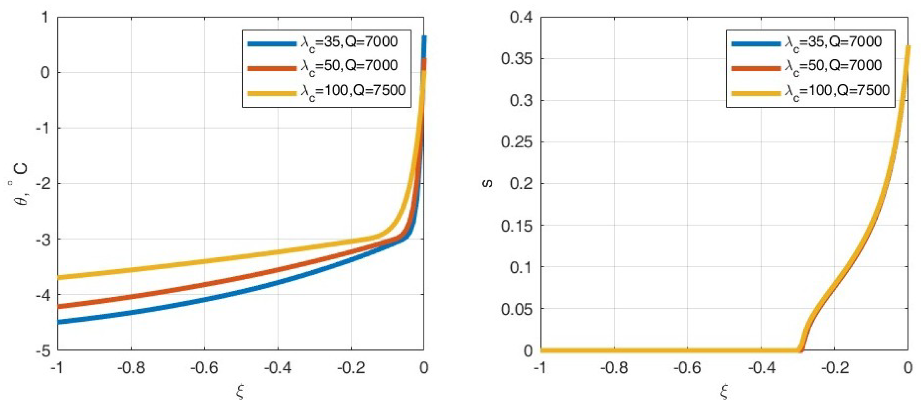
Figure 5.
Results of numerical modeling of temperature and water saturation changes for different values of
Figure 5.
Results of numerical modeling of temperature and water saturation changes for different values of
Disclaimer/Publisher’s Note: The statements, opinions and data contained in all publications are solely those of the individual author(s) and contributor(s) and not of MDPI and/or the editor(s). MDPI and/or the editor(s) disclaim responsibility for any injury to people or property resulting from any ideas, methods, instructions or products referred to in the content. |
© 2025 by the authors. Licensee MDPI, Basel, Switzerland. This article is an open access article distributed under the terms and conditions of the Creative Commons Attribution (CC BY) license (https://creativecommons.org/licenses/by/4.0/).
Copyright: This open access article is published under a Creative Commons CC BY 4.0 license, which permit the free download, distribution, and reuse, provided that the author and preprint are cited in any reuse.


