Entropy Field Structure and the Recursive Collapse of the Electron: A Thermodynamic Foundation for Quantum Behavior

1. Introduction—The Electron Beyond the Particle

In modern quantum mechanics, the electron is described as a point-like particle — a fundamental entity with no spatial extent, yet endowed with intrinsic properties: mass, charge, and spin. These quantities are not derived from internal structure or dynamic processes but instead introduced axiomatically into the formalism. The wave–particle duality, while elegant, remains interpretive: it allows electrons to behave as delocalized waves or localized particles depending on the measurement, yet it provides no mechanistic account of how localization occurs, nor why electrons possess the exact properties they do. Thus, while quantum theory accurately predicts outcomes of experiments, it does not reveal what an electron truly is. What, then, is an electron in the absence of observation — left alone in vacuum, governed only by the quantum vacuum field? It still manifests mass, radiates an electric field, interacts magnetically, and exhibits spin. These observable phenomena suggest a deeper field structure or internal entropy dynamic. In this work, we present a thermodynamic reformulation of the electron grounded in S-Theory — a unified framework in which physical properties emerge from recursive interactions between entropy fields.

1.1. Generalized Definition of Entropy in S-Theory

S-Theory begins with a primordial entropic background, $S_{\mathrm{\infty }}$: an unbounded, unstructured field composed of an infinite number of entropic quanta, the fundamental microscopic elements of the theory, as indicated in Figure 1. For mathematical convenience, individual entropic quanta are treated as elements of a complex potential field, whose real and imaginary components capture correlated and uncorrelated contributions. This allows wave-like interference and geometry to emerge from recursion, without postulating a separate quantum wavefunction. In $S_{\mathrm{\infty }}$, these quanta fluctuate freely without correlation or geometry, representing maximal entropy. Physical structure arises when subsets of these quanta become correlated, giving rise to three distinct correlation classes: (i) S_thermal — minimally correlated entropic quanta that generate thermal and background fluctuations; (ii) S_EM — highly correlated entropic quanta that organize into electromagnetic-like field structures; and (iii) S_core — maximally correlated entropic quanta that form stable, localized cores associated with mass. Energy and mass are not primitive; they emerge from these different correlation states. S_EM corresponds to organized field energy, S_core to localized mass structures, while S_thermal represents background heat and noise. We define the local entropy at position $\mathbf{r}$by counting the number of possible microscopic arrangements of entropic quanta within a finite local cell, subject to their correlation structure and boundary geometry. For 2D approximation,

(2)

Here, ${\mathsf{\Omega }}_S\left(\mathbf{r}\right)$is the total number of distinguishable microconfigurations of entropic quanta, decomposed into three contributions given by

(2.1)

corresponding to S_thermal, S_EM, and S_core, respectively.

• ${\mathsf{\Omega }}_{\mathrm{th}}$ counts micro configurations of entropic quanta that produce macroscopic thermal energy through random, minimally correlated arrangements.
• ${\mathsf{\Omega }}_{\mathrm{sEM}}$ counts field-structured micro configurations of entropic quanta arising from correlations linked to electric charges and magnetic field organization.
• ${\mathsf{\Omega }}_{\mathrm{Score}}$ counts mass-forming micro configurations of entropic quanta, representing maximally correlated clusters that behave as stable cores.

At each location $r,$ the total S-field arises from counts of correlated and uncorrelated entropic quanta. The resulting field structure — composed of S_core, S_EM, and S_thermal — is the macroscopic manifestation of these local correlations. In regions dominated by S_thermal, the definition reduces to the classical Boltzmann form. In structured regions, correlated quanta (S_EM and Score) reduce the number of accessible micro configurations, giving rise to organized energy fields and mass. This generalized entropy definition serves as the foundational expression for all subsequent derivations in S-Theory, unifying thermal entropy, electromagnetic field structure, and mass within a single entropic counting framework that encompasses both structured and unstructured components of physical reality.

This generalized definition does more than extend Boltzmann’s counting—it introduces geometry as an intrinsic outcome of entropy correlations. In classical statistical mechanics, entropy quantifies the number of microstates consistent with a given macroscopic energy, but it carries no information about spatial form. In S-Theory, however, the correlated entropic quanta (S_EM and S_core) not only reduce accessible micro configurations but also organize them in space, producing stable geometric patterns. These correlated fields act as sculptors of structure: S_core defines localized cores, while S_EM defines coherent surrounding fields, together giving rise to shapes such as atomic orbitals, molecular structures, and eventually large-scale cosmic forms. In this way, geometry itself is an entropic construct, emerging directly from the distribution and correlation of entropic quanta, not imposed by external equations. This shift—from entropy as a scalar descriptor to entropy as a shaper of structure—is the central conceptual advance of S-Theory.

To generate orbital fields in 2D, we work with the dimensionless capacity field

where S₀ is a fixed ground-state reference (peak of the total entropy density). Intuitively, the fraction of non-dimensional entropic density s ≈1 marks locations with many compatible micro-configurations available under the same mesoscopic constraints (high local accessibility), while s ≈ 0 marks nodes (strong constraints). Environmental influence is encoded by a driver s_c(r) that specifies where capacity can be unlocked (e.g., rings for s-like and dipoles for p-like structure). The state update is the local, pointwise map given by the recursive fractal equation,

(3)

interpreted as a constrained-maximum-entropy relaxation toward the next S-max pattern. Here, s_n= S/S₀ is the non-dimensional entropy density field s ∈ [0,1] at iteration n (initialized, e.g., with a 1s-like ground-state profile), s_c is a non-dimensional source term representing entropy input from the surrounding fields (constructed from the Sthermal and/or S_EM components), and s_n+1 is the updated field; under iteration, the map approaches a high-entropy configuration s_max. The superlinear self-term s² captures cooperative, contrast-enhancing growth—peaks tend to sustain, nodes persist—so that, together with a rim-localized s_c, the evolution is edge-driven (consistent with the annular area scaling A∝R²) rather than a global smear. Thus, the recursive equation (3) is essentially a phenomenological constrained-entropy ascent toward the next S_max macrostate.

Here, Score derives from the electron’s mass and acts as a gravitational anchor. S_EM forms a dynamic, spatially distributed shell — a Gaussian-like field whose amplitude and extent correspond to the observed electric charge. Sthermal surrounds and perturbs this system, carrying uncorrelated entropy from the quantum environment. Critically, we propose that measurement is a physical collapse — not a mystical boundary, but a thermodynamic threshold. When an external energy input (e.g., a photon) amplifies the S_EM and Sthermal components recursively (through a process we call Recursive Amplification of Sfield, or RAS), the system saturates. The S_EM field compresses and aligns with the Score core, yielding a collapse that produces definite quantities — charge, spin, position. In this view, quantum measurement is not arbitrary, but a structural transformation governed by entropy field thresholds.

This model offers several breakthroughs: i) Charge emerges from the saturated integral of the S_EM field, ii) Spin arises from the rotational geometry of the compressing S_EM shell, iii) Collapse becomes a predictable entropy field transition, not an undefined probabilistic jump, iv) and entanglement may arise via field correlations between overlapping Score fields across space. This work builds on our companion paper on hydrogen orbital formation and extends it by simulating the collapse process of a single free electron through successive RAS steps. The resulting predictions align with known physical constants and give physical meaning to abstract quantum attributes. We argue that quantum properties are not fundamental mysteries, but emergent thermodynamic consequences of entropy field dynamics. By grounding the electron in entropic structure, this work bridges statistical physics, thermodynamics, and quantum field behavior — and offers a new path toward a unified physical understanding.

To understand the electron not as a mysterious point particle but as a structured thermodynamic entity, we must first reframe our foundational assumptions. Instead of treating properties like charge and spin as primitive constants, we propose that they emerge from the underlying structure and dynamics of entropy fields. This requires a new framework — one that places entropy, not energy, at the root of physical reality. In the following section, we summarize the core tenets of S-Theory, the entropic field model that underpins this work and sets the stage for constructing a realistic, collapse-capable electron.

2. S-Theory as a Physical Expansion of Quantum Mechanics

2.1. A Brief Overview of S-Theory and Recursive Entropic Evolution

The development of S-Theory arose from a profound reflection on the limitations and open questions that still haunt modern physics. Quantum mechanics, despite its predictive success, leaves us with unsolved paradoxes—wavefunction collapse, quantum entanglement, and the emergence of classical reality from probabilistic fields. General relativity, though geometrically elegant, fails to incorporate thermodynamics or explain biological structure, information flow, or the arrow of time. The search for a unified theory has often resorted to increasingly abstract mathematical frameworks—such as string theory, loop quantum gravity, multiverse models—without resolving how complexity, replication, and consciousness emerge in a real, evolving universe. We propose that the missing piece is not a new dimension or force—but a reversal of the foundational assumption itself.

Instead of taking energy as the primary quantity, S-Theory begins with entropy: the tendency toward disorder, but also the hidden architecture behind structure, evolution, and intelligence. Our observable universe is energetic, yes—but underlying entropy fields guide every transformation, every structure, and every collapse. In this view, energy is structured entropy, space is the geometry of entropy correlation, and time is recursive entropic feedback (S_max-S_min-S_max cycle). S-Theory introduces three primary components: i) S_EM (Structured entropy of electromagnetic fields), ii) Score — frozen, memory-like entropy bound in particles or matter; a conserved structural core, iii) Sthermal — residual, unstructured entropy that manifests as heat, noise, or decoherence; the chaotic background. Together, these form the entropic trinity of physical reality. The recursive evolution of these entropy fields is governed by a simple, elegant, fractal-like equation (equation (3).

This simple yet powerful formulation models the emergence of structure, replication, and collapse—across scales. This entropic evolution logic is visually captured in the core recursive framework of S-Theory: The S-Ladder—a dynamic trajectory of entropy field evolution across all scales, as shown in Figure 1. It begins from S_∞, the infinite, unmeasured, uncorrelated entropy quanta of the quantum vacuum, where energy and structure do not yet exist. A localized recursive collapse initiates a descent to (S_max/E_min)—a saturated quantum coherence state with minimal correlation—followed by an expansion into (S_min/E_max) with maximum correlation, which in turn undergoes spontaneous symmetry breaking and recursive partitioning back to (S_max/E_min) as represented in Figure 1. Life, replication, complexity, and consciousness of OUR universe —all emerge from this return journey—an entropic climb from (S_min/E_max) back toward (S_max/E_min) and eventually merging again into the cosmic reservoir S_∞.

These two forward paths of Entropy S and Energy E are bounded by S_∞ (the entropy field of the vacuum) and T = 0 (absolute zero, the energetic floor of the universe). In this diagram (Figure 1), the left descent shows the universe’s thermodynamic fall, from cosmic entropy collapse to the ‘Big Bang’ that leads to the formation of matter and stars. The right ascent reflects the emergence of organized complexity: stars, Earth, molecules, and eventually life. In the solar system, crucially, the Sun (represented as a red dot in Figure 1) plays a pivotal role: by injecting energy (E_sun) into Earth, it reverses the E_min-path back toward E_max, triggering a corresponding inevitable reversal in the S-path (red arrow in the figure). This reversal from S_max towards S_min within living systems is what Erwin Schrödinger [1] referred to as “negative entropy” — a local entropy contraction against the cosmic flow, enabled by solar input and recursive feedback mechanisms. This is not accidental, but an inevitable thermodynamic symmetry of a universal entropic cycle [1,2,3]. In this view, life is not a statistical anomaly but a required resolution in the larger recursive equation: a pathway from disorder back to structure via memory fields, S_thermal fluctuations, and S_max convergence. This is the Ladder of Entropic Evolution — not climbing out of chaos but recursively spiraling back toward S_∞ through order, and it unifies quantum events, biological replication, and gravitational collapse under one thermodynamic cycle [4].

3. Generating the Entropy Field Model of an Electron

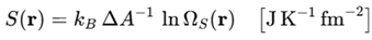
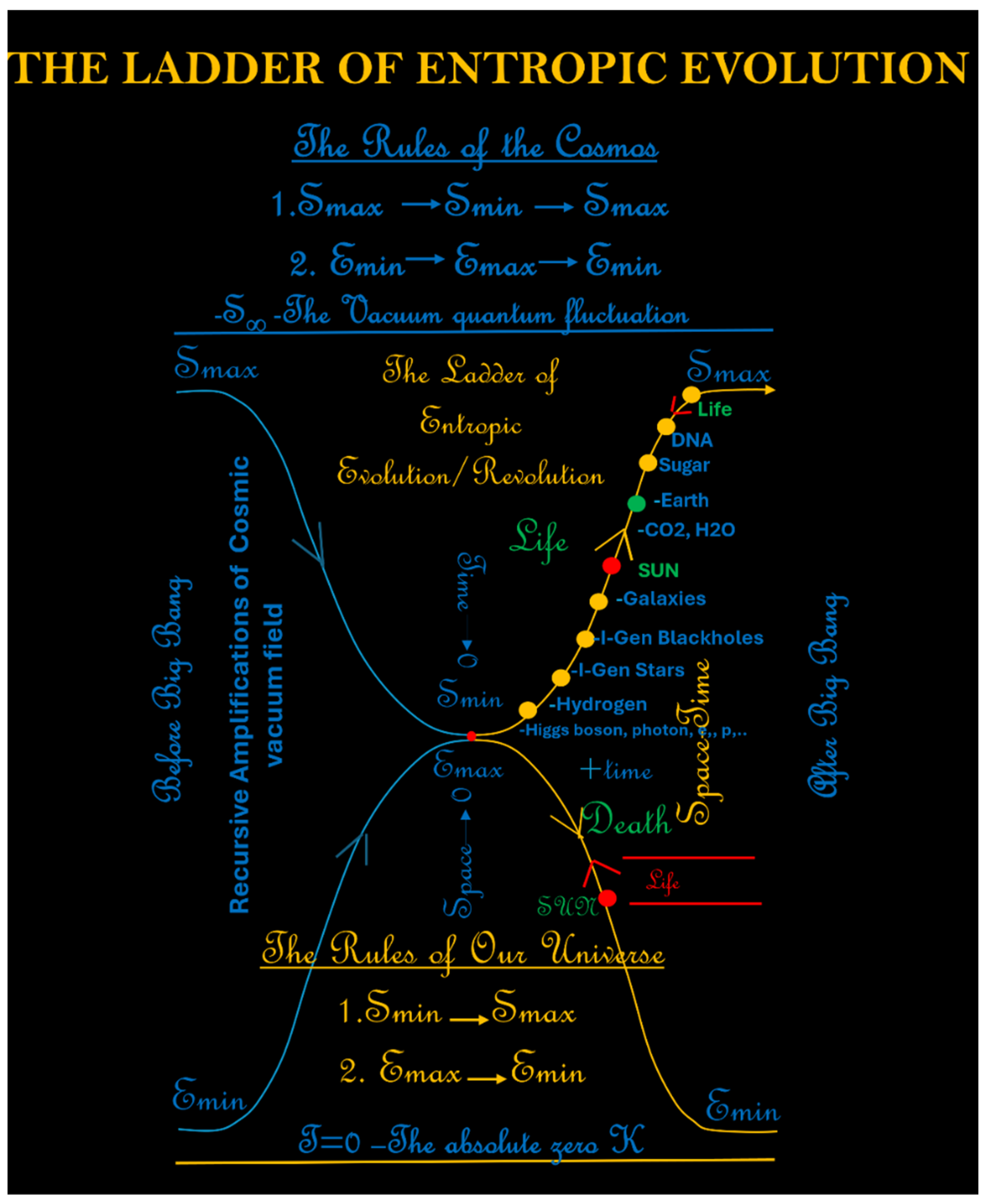
In S-Theory, the electron’s mass is not treated as a scalar quantity or a point object, but rather as a structured entropy field — a localized distribution of entropy density, centered at the origin and falling off radially. This core field is denoted Score(r) and represents the internal collapsed identity of the electron arising from its rest mass.

3.1. Mathematical Formulation of Score from Electron Mass

(i) The Score Field – Entropy Core of the Electron

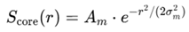
We define the core entropy field of the electron, denoted as Score(r), to represent the structured entropy arising from the electron’s rest mass.

(2)

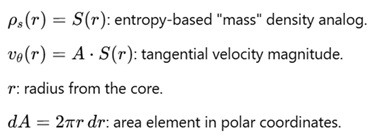
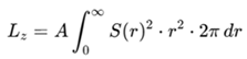
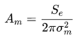
Where: A_m is the normalization constant for entropy density (not mass), σ_m is the characteristic width of the Score field.

(ii) From Mass to Entropy: Core Logic

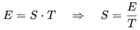
According to S-Theory, mass is structured entropy. Following Einstein:

E = m_ec² and S = E/T ⇒ S = m_ec² /T

(3)

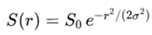
where T is an effective entropic temperature — a measure of entropy freedom (low for stable mass). This structured entropy is not spread across all space but localized into a dense core — the Score field, which stores the “collapsed identity” of the electron. This entropy is highly localized, meaning the field must peak sharply and decay rapidly — consistent with a Gaussian profile. The spatial width σ_m is not arbitrary. It is chosen based on the Compton wavelength λ_C of the electron:

σ_m = λ_C =ℏ/m_ec ≈ 3.86×10⁻¹³ m

(4)

This defines the natural localization radius of the electron’s core entropy. This corresponds to the natural quantum length scale over which the electron’s wavefunction — or here, entropy field — is confined.

(iii) Normalization of Score Field

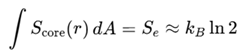
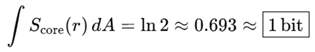
We now normalize Score such that its total integrated entropy corresponds to Se = k_B ln 2, representing one bit of fundamental entropy — the minimal quantum configurational entropy associated with a spin-½ particle (Ω = 2 microstates). That is,

(5)

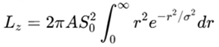
In polar coordinates:

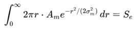(6)

This evaluates to:

(7)

Using:

k_Bln2 ≈9.57×10⁻²⁴ J/K

σ_m=λ_C=3.86×10⁻¹³ m

We obtain:

Am ≈ 9.57×10⁻²⁴/2π (3.86×10⁻¹³)² ≈1.02×10² J/K

(8)

(iv) Physical Interpretation and justification

This construction yields the Score(r) field as a sharply peaked entropy density centered at the origin and localized at the Compton scale. Its integral gives one bit of structured entropy, meaning: i) Mass becomes a localized entropy configuration, not a constant, ii) The field is sharply confined (~10⁻¹³ m), representing the collapsed identity of the electron, iii) Entropy is quantized in discrete bits, even for elementary particles. This approach reinterprets mass as frozen, structured entropy, embedded in space via a measurable field distribution.

This field represents the irreducible structured identity of the electron — the entropy signature associated with its mass. As shown in Figure 2 (red color field), this field sharply peaks at the center and decays radially. Now we have a Score that is clearly defined as an entropy field, not a mass density. σ_m is set by Compton wavelength, not arbitrary. The normalization yields a physical entropy unit (e.g., 1 bit, or k_Bln2). This Score represents a normalized Gaussian entropy density, centered at the origin, which defines the electron’s collapsed mass configuration. The field integrates to k_B ln 2 and is localized at the Compton scale (~10⁻¹³ m), establishing mass as a structured entropy phenomenon in the S-Theory framework.

(v) Why ln 2? The Identity Bit of the Electron

In S-Theory, every stable quantum system must possess a minimal entropy signature anchoring its individuality. For the electron, with spin-½ and Ω = 2 states:

S = k_B ln Ω = k_B ln 2=0.693 k_B

(9)

This is not thermal entropy but ontological entropy — a measure of how many internal configurations a collapsed system can realize. This idea, consistent with quantum information theory, provides a deep bridge between thermodynamics and identity: The Score field encodes the electron’s “1 bit of being.”. This assignment does not imply thermal entropy in the conventional sense, but instead defines a minimum ontological entropy associated with the electron’s existence as a distinct, indivisible fermion. In the context of S-Theory, this unit entropy anchors the Score field, allowing us to treat the electron’s mass as a localized, structured entropy field normalized to a fundamental quantum of identity. This normalization not only aligns with Boltzmann entropy and quantum spin logic but also provides a consistent base for comparing and interpreting the electron’s associated fields — including the spread entropy of charge (Section 3.2) and the dynamic thermal field during interaction (Section 3.3). In dimensionless units (e.g., setting k_B=1 in natural units), this is:

(9)

Thus, the electron’s mass is reinterpreted as a field that contains exactly 1 bit of structured entropy — distributed in space such that its Score field integrates to ln2. In practice, some literature (especially in quantum information theory) approximates 1 bit entropy as “2” when expressed as Ω (number of microstates), which gives: S = lnΩ = ln2 ⇒ Ω=2. So, we are not integrating to a value of “2” directly, but rather: to k_Bln2 in SI units, or 1 bit in information units, or 0.693 in pure math units. We present the mass of the electron as an entropy field (Score), peaked at the center, whose total integral is k_Bln2— representing one bit of structured entropy associated with the collapsed electron identity.

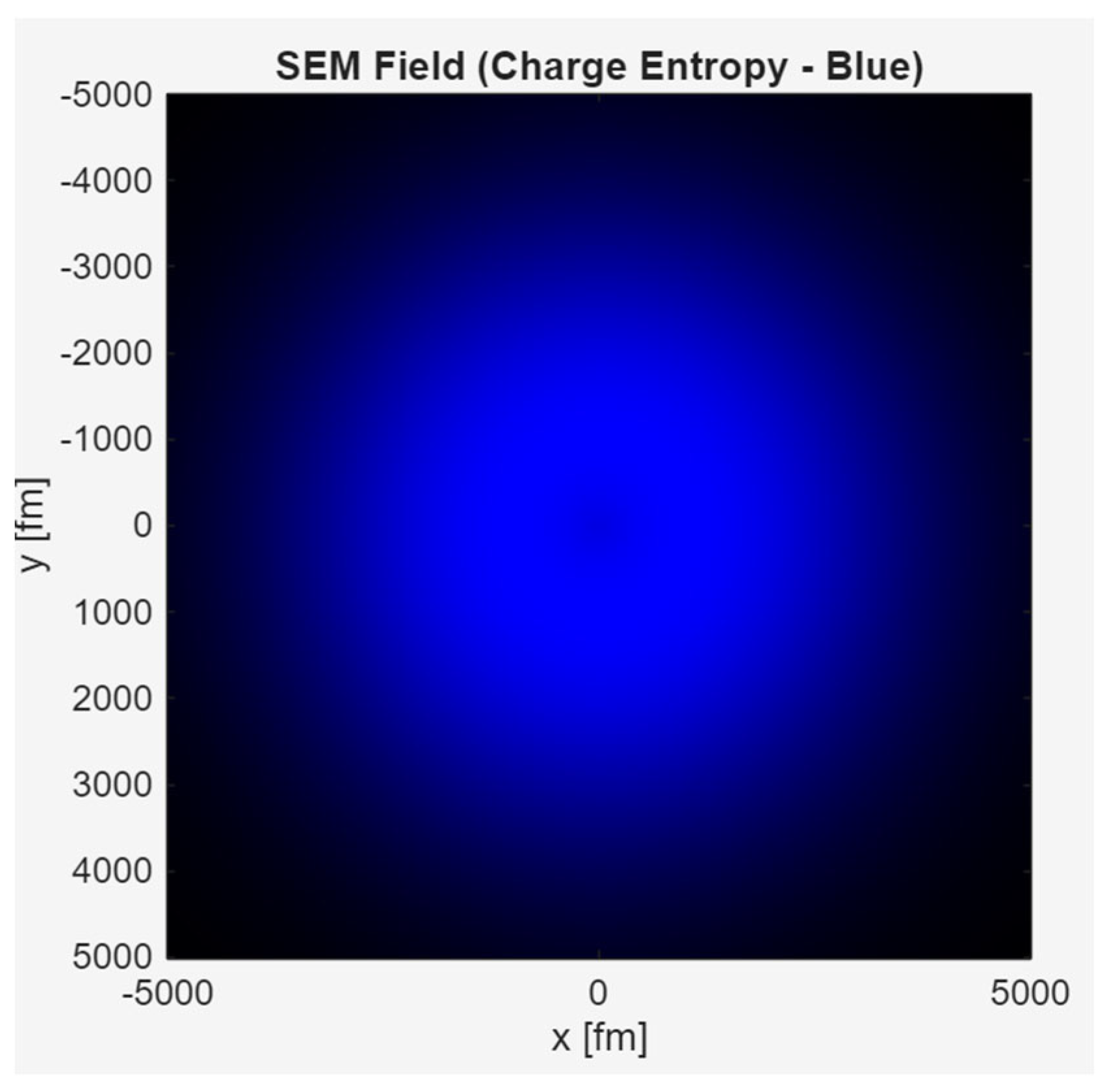
3.2. Mathematical Formulation of S_EM from Charge

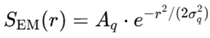
The S_EM field represents the distributed electromagnetic entropy associated with the electron’s electric charge. Unlike the Score field, which is sharply localized due to mass, the S_EM field is spatially broader and reflects the outward entropy radiation of charge. We model it using a radially symmetric Gaussian:

(10)

Where: A_q is the normalization constant linked to electromagnetic entropy density, σ_q is the characteristic spread of the field (typically σ_q > σ_m).

(i)From Charge to Entropy: The S-Theory Logic

In classical electrodynamics, an electric charge creates a radial Coulomb field that stores energy. In S-Theory, energy is interpreted as structured entropy:

(11)

Thus, the Coulomb field around the electron gives rise to a corresponding spread entropy field, S_EM, which encodes the spatial distribution of electromagnetic potential in thermodynamic terms. Rather than normalizing this field to the charge magnitude ∣q_e∣, we normalize it to a meaningful entropy quantity. To ensure consistency with the Score field (Section 1), we define the total entropy in the S_EM field as:

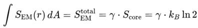(12)

Here, γ is a dimensionless scaling factor reflecting the broader spatial influence of charge compared to mass. Typically, γ>1.

(ii) Choice of Spread Width σ_q

The spatial spread of the S_EM field is selected to reflect the more diffuse nature of electromagnetic fields. Rather than using the classical electron radius, we define:

(13)

where

(14)

λ_C is the Compton wavelength, and η is a scaling factor. Choosing η=4, we obtain:

σ_q =4⋅λ_C ≈ 1.54×10⁻¹² m

This ensures that the S_EM field is smoother and more extended than the Score field, in accordance with observed electromagnetic behavior.

(iii) Normalization Constant

Given the Gaussian form of the S_EM field, the entropy normalization gives:

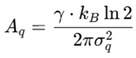(15)

For example, with γ=3 and the above value of σ_q, we obtain:

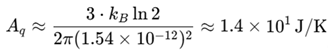(16)

This yields a broad entropy field that smoothly decays with distance and contributes significantly to the total entropy structure of the electron.

Figure 3. S_EM Entropic EM field distribution of Electron.

Figure 3. S_EM Entropic EM field distribution of Electron.

(iv) Estimation of microstates of S_EM: Comparison to Score

In the previous section 2.2, we derived

Score = k_BlnΩ = k_Bln2 ≈0.693 k_B

(17)

This corresponds to 1 bit and reflects collapsed identity (a binary quantum choice: spin-up/down, particle/antiparticle, etc.). Now: What Should S_EM Represent? The S_EM field is: i) spread out, not collapsed ii) derived from electromagnetic field energy iii) not a binary state, but a continuum of influence, so it shouldn’t be just “1 bit” like Score. It should encode more entropy — a distributed informational cloud, not a defined choice.

When we set γ=3, we Are Saying:

(18)

This is not 3 bits, but:

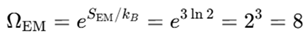(19)

Interpretation: If the Score field represents an electron’s collapsed identity — 1 bit (Ω = 2), then the S_EM field represents a more delocalized, entangled field — encoding Ω = 8 possible microstates (i.e., 3 bits of information). What does this tell us? The entropy content of S_EM is higher not because it’s more “informative” in a collapse sense, but because it’s spread across more degrees of freedom. While Score = collapsed, bounded, S_EM = expanded, radiative, and contains multiple field configurations or “degrees of potential interaction”. So, we might interpret: Score as existence entropy (a single quantum identity), S_EM as interaction entropy (the field’s available entangled micro-configurations with space).

(v) What if Gamma Were 5 Instead?

So γ is directly scaling the microstate count of the SEM field:

(20)

It gives us a semantic handle on field complexity.

Final Summary:

Field	Total Entropy S	Bits	Microstates Ω	Meaning
Score	kBln2	1	2	Binary identity (collapse)
SEM	γ⋅kBln2	γ	2γ	Distributed EM interaction entropy

So, with γ=3, SEM carries 8x more microstate potential than Score.

(vi) Physical Basis of γ — Linked to Spatial Entropy Volume

Entropy depends not only on the amount of energy (charge field), but also on how spread out it is. We define:

(21)

So: a larger spatial spread (larger σ_q) means more possible configurations for the field → higher Ω_EM, higher γ. A tightly confined field (small σ_q) means fewer options → smaller γ. So γ is directly tied to the spatial entropy volume:

(22)

We can think of it as a “configurational volume ratio. What happens to S_EM after the collapse? When a measurement occurs (e.g., detecting charge or interaction): i) The spread entropy collapses to a localized structure (like a Score-type). ii) the system selects one of the Ω microstates from the S_EM field ii) So the measured charge corresponds to 1-bit output (Yes: charge detected; No: not detected). So, after the collapse:

(23)

The rest of S_EM’s entropy radiates outward or decoheres, just like a wavefunction collapse in QM.

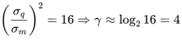
(vii) Justification of γ = 3 (vs. 10)

Our choice of γ = 3 is: not a guess, but a provisional assignment based on a physical scale:

σ_q=4⋅λ_C

(24)

Since σ_q/σ_m=4 and entropy scales with area:

So γ ≈ 3–4 is reasonable based on spatial scaling. If we had chosen: σ_q=10σ_m → γ ≈ log(2x100) = 6.6, this would imply 6–7 bits of field complexity — valid only if the electron is embedded in a very high-energy or noisy EM environment. So: γ is not fixed by charge, but by field geometry and available spatial entropy before collapse. So, γ is not arbitrary but tied to the spread radius of the entropy field, charge is constant, but entropy associated with that charge depends on space and configuration freedom, after measurement, only 1 bit remains — the rest is dissipated or encoded elsewhere. So γ captures the pre-collapse entropy potential of the electron’s EM field.

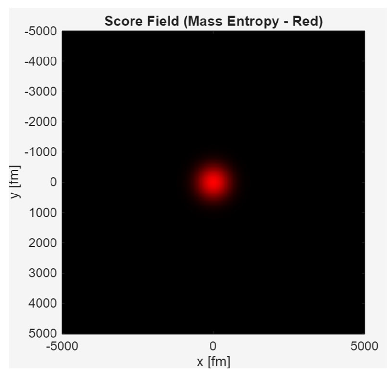
3.4. The Sthermal Field: Entropic Interaction Between Structure and Environment

In the S-Theory framework, the entropy field of a fundamental particle such as the electron is not fully described by mass (Score) and charge (S_EM) alone. These fields represent intrinsic, localized (Score) and spatially extended (S_EM) components of structured entropy. However, the third and often overlooked dimension is interaction entropy — the distributed and fluctuating entropic field arising from the electron’s coupling to the surrounding environment and vacuum fluctuations. We call this field Sthermal, short for Structured Thermal Entropy.

(i) 

Origin and Necessity of Sthermal

Whereas Score is derived from the concentrated entropy due to rest mass and S_EM from the spread associated with the electromagnetic field, Sthermal arises from external interactions — including temperature-dependent noise, quantum vacuum fluctuations, and photon scattering. It captures the entropy flow into and out of the electron’s system boundary. This makes Sthermal the key dynamic component that determines whether the electron collapses (measurement), radiates (scattering), or remains in a superposed, thermodynamically stable state. Traditionally, quantum mechanics assumes idealized closed systems and primarily models probabilities via the wavefunction. In contrast, S-Theory explicitly recognizes the system’s coupling to its entropic surroundings, leading to a more complete and physically grounded model of the electron as a dynamic structure embedded in a sea of entropy. This aligns closely with open quantum systems and thermofield dynamics, yet goes further by defining a scalar field that measures the residual entropy potential surrounding a quantum object.

(ii) 

Mathematical Formulation of the Sthermal Field

The Sthermal field shown in Figure 4 is constructed as a low-amplitude, wide-spread Gaussian random field added to the entropy profile. Unlike Score and S_EM, which are symmetric and physically defined by core parameters (mass and charge), Sthermal is non-symmetric and randomly modulated, representing microscopic stochasticity and interaction history. We define the Sthermal field over a 2D domain using a low-frequency filtered random noise modulated by a Gaussian envelope:

(25)

Where: smooth_rand (x, y) is a low-pass filtered 2D random noise (e.g., convolution with a Gaussian kernel), σ_th is the thermal spread radius, much wider than S_EM or Score, A is a small amplitude scaling factor, ensuring Sthermal does not dominate in isolation but strongly modulates during collapse events, the units are normalized entropy density per unit area. This field is then normalized to a maximum of 1 before visualization or summation into the RGB field.

(iii) 

Physical Interpretation: The Missing Link in QM

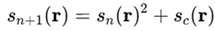
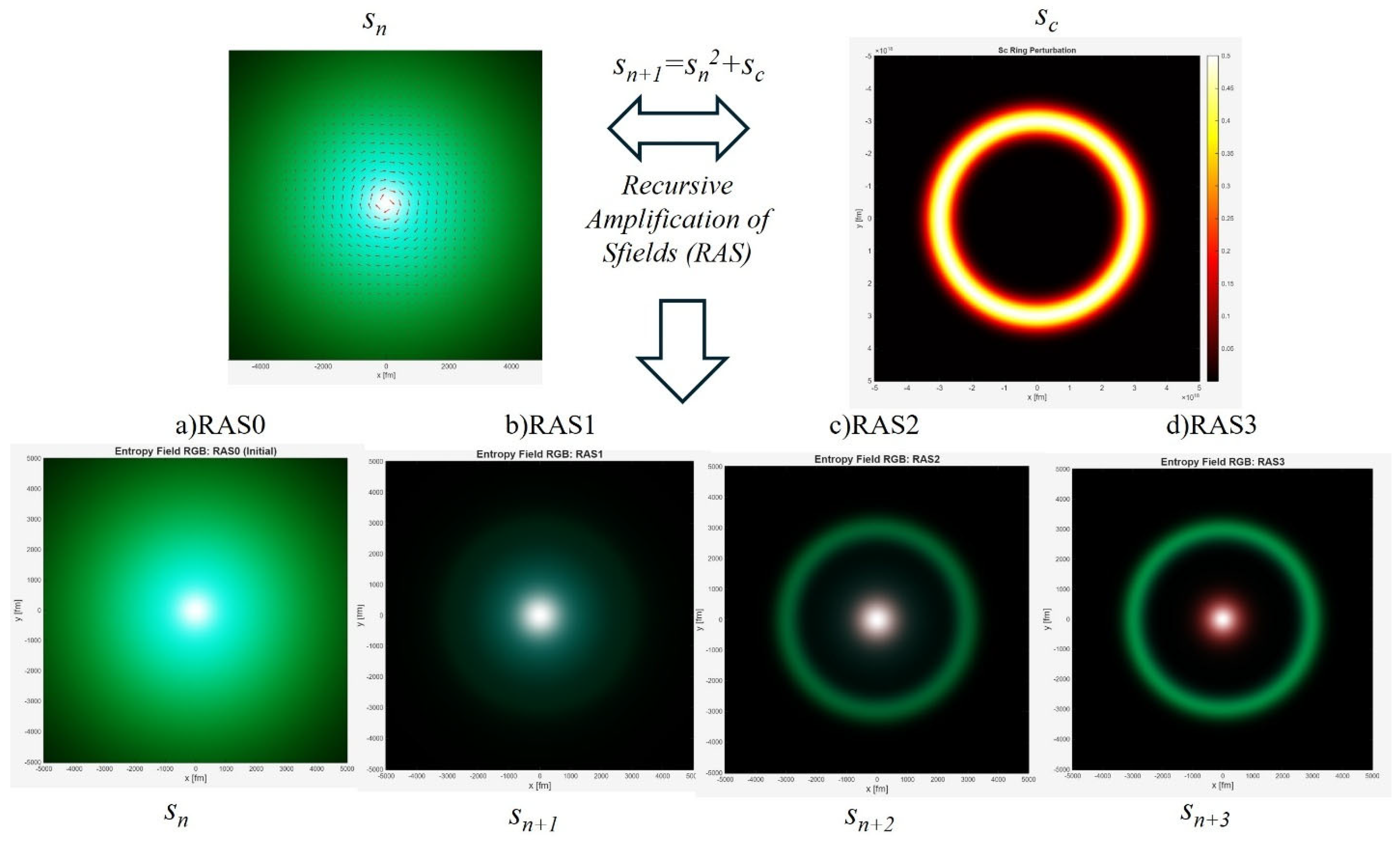
The Sthermal field (Figure 4) plays several vital roles that are ignored or marginalized in standard QM: i) entropy exchange: It captures the entropic flow to/from the environment, which is central to the measurement process ii) collapse sensitivity: the moment a high-energy photon enters the Sthermal field, recursive amplification of Sfield (RAS) with S_EM can drive the system toward collapse, iii) entropic equilibration: It defines the thermal envelope in which Score and S_EM are modulated — without it, any energy-based picture misses the stochastic interactions needed for life, measurement, or evolution, iv) time-evolution context: As shown in later sections, Sthermal governs local entropic time, as used in EPS (Entropy Positioning System [5]), defining the effective “aging” or dynamic change of field structure over time. Thus, in S-Theory, Sthermal is not optional. It is the thermodynamic gradient and stochastic scaffold without which no real system (including electrons, molecules, or brains) can evolve or respond to measurement.

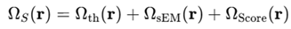
3.5. Combined Entropic Field of an Electron

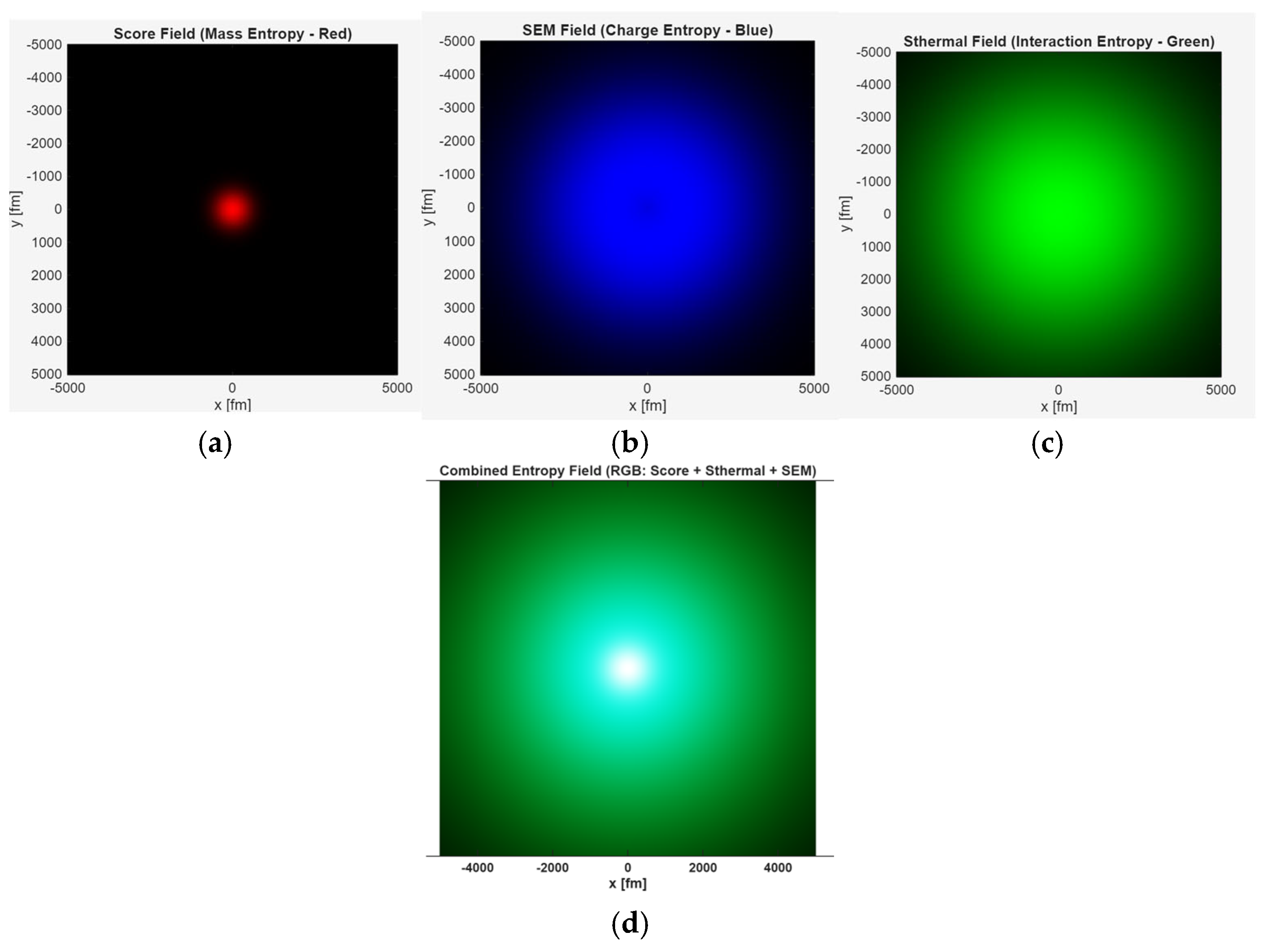
Figures 5a–c present a summary of these three entropic subfields individually in color-coded visual form: Score in red, S_EM in blue, and Sthermal in green, each emerging from the same radial coordinate space but expressing different spatial scales and intensity gradients. Figure 5d is the combined entropy field of the electron (RGB Composition). This RGB fusion total image synthesizes the three entropic components into a single composite field given by equation (26).

(26)

The red (mass), green (thermal), and blue (charge) channels are superimposed, forming a complete entropy structure of the electron. The bright white center signifies the peak of recursive entropic amplification, where all three fields converge — a region of maximum coherence and minimum uncertainty. This unified representation provides a visual and thermodynamic map of the electron as a structured entropy field, central to the S-Theory reinterpretation of quantum mechanics. In Figure 5d, the Sthermal field appears as the green component, forming a diffuse glow enveloping the sharper Score (red-turned white in the combined image) and S_EM (blue) fields. Its presence transforms the otherwise symmetrical Score–S_EM model into a realistic, fluctuating, field-interactive system, opening the door to a thermodynamic explanation of uncertainty, wavefunction collapse, and decoherence.

(i) Estimation of microstates of S_thermal: Comparison to Score and S_EM

Based on prior modeling, the S_EM field is linked to the Score field by a scaling factor γ=3, leading to S_EM=3 x Score and an associated increase in microstates from Ω_core=2 to Ω_EM=2³=8. For the Sthermal field, which has the most significant spatial extent and represents the thermodynamic residue of interaction, we estimate a higher scaling factor α ≈ 5–8 resulting in Sthermal=α⋅Score. This yields a microstate range of Ω_thermal = 2α = 32 to 256. Thus, the Sthermal component carries the dominant share of entropy and microstates in the complete Sfield structure. Conceptually, the collapse process compresses this Sthermal cloud and the S_EM field toward the Score core, and leaves behind a coherent, spinning entropy structure—giving rise to measurable properties like charge and spin. This expanded entropy perspective, uniquely enabled by S-Theory, restores the missing thermodynamic dimension neglected by traditional quantum mechanics and provides a more complete framework for understanding measurement, decoherence, and particle identity.

4. S_EM Field Structure with Spin

4.1. Rotational Spin Field: Mathematical Formulation

To embed spin into the S_EMfield we discussed in section 3, we define a tangential vector field (i.e., field lines circulating the core) with magnitude proportional to the entropy field. The vector field v⃗_s is constructed as:

(27)

This creates a counterclockwise (CCW) circular rotation around the origin, representing spin-up, x/r, y/r, are unit tangent directions at radius r, ais the normalization constant, whose value is chosen so that the total angular momentum of the field equals ℏ/2. It captures the localized rotational motion of the entropy field that gives rise to quantum spin.

(i) 

Total Integrated Spin and Normalization Constant

We calculate the total angular momentum of the entropy-based spin field as:

(28)

Where:

This gives

(29)

Substituting

(30)

We get

(31)

This evaluates to

	(32)
	(33)

In the simulation, we choose

• ℏ=1.055×10⁻³⁴J s
• S₀=1(dimensionless, normalized)
• σ=10 fm=10×10⁻¹⁵ m

Resulting in:

A ≈ 4.79×10⁶ (SI units) (34)

This ensures that the total angular momentum stored in the entropy-rotating field equals the electron’s spin: Lz =ℏ/2

4.2. Spin-Up and Spin-Down Representation

The sign of the spin vector field determines the spin direction:

(35)

Figure 6 shows the Electron S_EM field we generated in the previous section (Figure 5d) with overlaid spin vector fields derived from section 4.1. Figure 6a (Left): Spin-Up (counterclockwise vector circulation). Figure 6b (Right): Spin-Down (clockwise circulation). In summary, in standard quantum mechanics, spin is treated as an intrinsic property — a fundamental quantum number assigned without origin. In contrast, S-Theory proposes that spin arises naturally from the rotation of the structured entropy field (S_EM) surrounding the electron’s core (Score). When a tangential vector field is applied to the S_EM — creating a circulating entropy density around the Score — a coherent rotational structure forms. This rotating field, once normalized to yield angular momentum ℏ/2, generates the emergent phenomenon we observe as spin-½. During collapse, this rotational entropy localizes into a sharply defined peak, yielding a measurable spin state and conserving angular momentum, which is discussed in section 5.

We have shown that the spin of the electron in S-Theory is not an abstract quantum number, but a direct result of distributed entropy field rotation, modulated by the local field structure. The total spin emerges from integration of the rotational entropy field, and the exact quantum value ℏ/2 is recovered through normalization. This marks a significant shift in how quantum properties can be physically visualized and simulated — bringing us one step closer to a unified entropic theory of particles, structure, and dynamics.

5. Entropy-Based Collapse of the Electron—A Recursive Amplification Structure (RAS)

Having constructed the total entropy field of the electron — composed of the core entropy (Score), the electromagnetic entropy cloud (S_EM), the ambient entropy fog (Sthermal), and the rotational spin vector field — we are now positioned to investigate the critical question: what happens when this entropy field is perturbed or measured? The complete initial state is shown in Figure 7a as Sn (RAS0), where the electron’s full Sfield is visualized as an RGB composite with embedded spin vectors. At the heart of this section lies a bold hypothesis: electron collapse is not a mystical event, but a recursive thermodynamic phenomenon, governed by the same law that drives emergence — the recursive amplification of the Sfield (RAS) mechanism of S-Theory.

5.1. Why RAS? A Thermodynamic Recasting of Collapse

In standard quantum mechanics, wavefunction collapse is an axiomatic process: a particle’s probabilistic wave abruptly localizes upon observation. Yet this notion lacks a physical mechanism — why or how collapse happens is left unanswered. The measurement problem remains one of the most elusive paradoxes of physics. S-Theory replaces this postulate with a process: recursive entropy amplification. Instead of an abstract projection, collapse is modeled as a real-space interaction between an electron’s entropy field and an external perturbation — an s_c field — producing dynamic feedback that amplifies some entropy structures and dissipates others. Mathematically, this is expressed by the core evolution equation: s_n+1=s_n²+s_c (2). This is not a metaphor, but a nonlinear recursive interaction rule that defines the electron’s response to high-energy input.

5.2. What Triggers Collapse?

In real measurements — whether in scattering, detection, or excitation — collapse is typically initiated by a high-energy photon or interaction field. This event is extremely short-lived but locally intense. The spatial size of a photon wave packet often exceeds that of an electron by several orders of magnitude. Yet the interaction zone is confined: the core entropy of the electron (Score) provides a localized anchor, while the incoming field perturbs its surrounding S_EM and Sthermal layers. To model this, we inject a structured entropy field s_c — a circular entropy ring as shown in Figure 7b — surrounding the electron core. This field simulates the entropy profile of an incident high-frequency photon or external EM perturbation.

5.3. Why a Ring? Spatial Logic of Measurement

A key insight is that collapse is not merely energy absorption, but spatial reconfiguration of entropy density. A photon interacting with an electron does not strike a point — it perturbs the surrounding EM field. Thus, the s_c field is modeled as an annular entropy ring, representing the entropy input distributed around the electron at a radius of maximum interaction, consistent with the observed size scales of photon–electron interactions. This structure ensures that the RAS process acts not at the center (s_core), but in the outer entropy field (s_EM + s_thermal), triggering a recursive redistribution that feeds back inward.

5.4. What is s_c? A Perturbation of Entropic Origin

The s_c field is constructed as a Gaussian ring of entropy density — incorporating both thermal and EM contributions: i) s_thermal: representing ambient entropy noise or vacuum fluctuations, ii) s_EM: a focused external field such as a photon pulse. s_c is therefore not a specific particle, but a generalized entropic perturbation. It reflects the entropy structure of the interaction source — whether light, field, or force — and becomes the seed for amplification.

5.5. Collapse as Recursive Amplification

The RAS mechanism is now engaged: the initial electron entropy field (s_n), composed of s_core + s_EM + s_thermal, interacts with s_c. The nonlinear recursion begins: i) where s_n and s_c are in-phase or aligned, their entropies amplify, ii) where they interfere destructively, entropy dissipates, iii) the total field reorganizes into a new configuration s_n+1. This process continues recursively, converging when the field saturates — when the entropy density at the s_core region equals or exceeds a collapse threshold. At this point, we define collapse: a focusing of distributed entropy into the core, with expulsion or dissipation of the residual field (e.g., s_thermal).

6. Collapse of Electron: A Recursive Entropic Interpretation from Field Profiles

6.1. Non-Dimensional Formulation and Numerical Setup

Let S (x, y) denote an entropy-density field with units J·K⁻¹·fm⁻². We fix a single reference scale from the baseline state (RAS0), S₀ = max (x, y) S_tot,₀(x, y) and work with non-dimensional fields s_n (x, y) =S_n (x, y)/S₀, sc (x, y) =Sc (x, y)/S₀. The update is applied pointwise on a uniform 2-D grid as the non-dimensional map given in equation 2 with no per-step re-normalization. (Equivalently, in dimensional variables Sn+1=Sn²/S₀+Sc, which makes the role of S₀ explicit). Domain and discretization. We use (x, y) ∈ [−L, L]²(fm) on a uniform grid of size N×N times with Δx = Δy and area element dA=Δx Δy. (Values used in the figures: L=5000 fm, N=400). Source term. The ring-like perturbation is introduced as a dimensionless field s_c (x, y) =c_frac s^c (x, y), where s^c is a unit-peak shape (e.g., Gaussian ring), and cfrac∈ (0,1) controls its strength. Recovery of physical units for observables: When reporting integrated or moment-type quantities, we first restore units via S=s S0 and integrate with the same dA. The spin-like moment is then normalized so that Lz=ℏ/2. The charge-like integral is reported in Coulombs after a single calibration at the stated RAS step. This keeps the recursion dimensionless while ensuring all reported observables carry correct physical units. Visualization and units. Spatial axes are in fm. Field magnitudes are plotted as s=S/S₀ (dimensionless, common scale, additive view). ROI summaries are reported as mean s over the interval (dimensionless). Spin Lz is in J·s; charge-like integrals are in C. Note. The field s is “probability-like” (non-negative and dimensionless) but is not a probability density unless explicitly normalized by its area integral—sanity checks. We verify (i) additivity s_tot=s_core + s_EM + _Sthermal pointwise, and (ii) consistency of the area element dA across all integrals. These checks ensure dimensional consistency throughout.

6.1. Simulation of Sfield from RAS0 to RAS3 (Field Images)

Figure 7a-d illustrates the full-field evolution of the electron’s entropy structure during recursive amplification (RAS) collapse. Figure. 7a shows the initial entropy field (RAS0), where the core (s_core), charge field (s_EM), and thermal field (s_thermal) form a smoothly blended, diffuse s_max structure. As RAS progresses in panels (b) through (d), entropy density compresses inward while outer structures sharpen — forming coherent radial shells. In RAS1, the central s_core begins to dominate visually, and by RAS2, the entire field exhibits clear bifurcation between a dense entropic core and a high-gradient ring. RAS3 reveals the signature of collapse: a highly saturated central entropy density surrounded by structured field lobes — confirming that the electron’s measurable attributes emerge from recursive entropy focusing.

Notably, the luminous green ring visible in RAS2 and RAS3 represents a sharply structured s_thermal field, encircling the compressed s_core and s_EM. This outward-diffusing s_thermal carries entropic energy from the core and acts as the thermodynamic interface with the measurement environment. It is this ring — rich in entropy but weak in structural anchoring — that first reaches the detector or measurement system, triggering the collapse of the inner fields into observable quantities like charge, mass, or spin. In this view, measurement is not a collapse of the wavefunction but a natural entropic diffusion from structured order (s_core + s_EM) into thermal interaction (s_thermal), followed by irreversible entanglement with the observing system. The field evolution here provides the most precise visual and thermodynamic map of what measurement truly means in physical reality.

6.2. Simulation of Sfield from RAS0 to RAS3 (Sfield Density Profiles)

We work with the non-dimensional field s=S/S₀ for all updates and plots; physical units are restored only when reporting observables via S=sS₀ with a single area element dA.

(i) Figure 8a: Baseline Entropy Profile (y = 0 Line Cut): Figure 8a shows the radial entropy field profile of the electron, taken along the x-axis at y = 0. This is the reference state before any perturbation or measurement. The black curve represents the total entropy field s_total=s_core + s_EM +s_thermal. This is the total information field defining the electron’s identity, interaction, and ambient coupling. Each colored curve corresponds to one component: i) Red: Score, the entropy field associated with mass, sharply localized around the origin (x = 0). This narrow peak reflects the dense, bounded entropy of the electron’s “collapsed” existence — the s_core field derived from Compton-width Gaussian (Eq. 4). ii) Blue: s_EM, the entropy from charge-based electromagnetic interaction. It is broader than the s_core, derived from Eq. 10, with width σ_q=4 λ_C, and reflects the more spread-out field influence. iii) Green: s_thermal, the broadest field, capturing ambient entropy interactions (background photons, stochastic field noise), modeled with a Gaussian of even larger spread. While less dense, it plays a crucial role in the collapse. This trinity of fields (s_core, s_EM, and s_thermal) forms the entropic structure of the electron. Although s_EM and s_thermal are spatially broad, their entropy density is lower compared to s_core. This distinction is critical: it is not just the spatial extent, but the local entropy density that determines how collapse unfolds.

ii) Figure 8e: Tangential Spin Velocity Profile from s_EM: The corresponding spin field (Figure 8e) plots the tangential velocity profile derived from the rotation of the s_EM field, projected along the same axis. Unlike s_core, which is static and non-rotating, s_EM carries a directional entropy flow — the root of electron spin in S-Theory. Here we observe: i) A wide, smooth bell-shaped profile indicating that spin is not sharply localized, ii) The maximum spin velocity is around the mid-region, confirming that spin is a field effect, not a core identity. This redefines spin: not as an abstract quantum number, but as a distributed rotational flow of entropic interaction, physically visualized and dependent on s_EM structure. Together, Figure 8a and 8e provide a clear baseline: i) the electron is not a point, but an extended entropy structure, ii) its mass (score) is tightly bound and carries high local entropy density, iii) its charge field (s_EM) is broader and rotating — the source of spin.

iv) RAS Step 1 — Beginning of Collapse: Compression and New Structure Formation: In Figure 8b, we present the result of the first recursive amplification step (RAS1) applied to the electron’s non-dimensional entropy field using the update rule: s_n+1=s_n²+s_c (2). This process simulates the effect of an external entropy perturbation s_c — such as a measurement photon — interacting with the native entropy field of the electron. The effects are striking: i) Central Compression of Entropy: the total entropy curve (black) shows a marked narrowing toward the origin compared to the baseline (Figure 8a). This signals the onset of collapse, where entropy is being drawn inward, amplifying its central density through recursive feedback. ii) Merging of s_EM and s_thermal: The blue and green curves, previously distinct (representing charge and thermal entropy fields), now collapse into a single, nearly overlapping profile. This reflects a loss of their separate field identity — a key signature of collapse — while still remaining broader than the red s_core. iii) Emergence of side lobes: A significant new phenomenon appears: side lobes — secondary peaks symmetrically located away from the core. These likely represent redistributed and amplified Sthermal entropy, pushed outward as central compression proceeds.

This may correspond to potential interaction zones or field residues post-collapse. iv) Formation of a core–wall structure: The overall profile now begins to resemble a two-zone system: A compressed core region near x = 0, surrounded by a high-entropy “wall” — marking the first formation of structured spatial boundaries in the entropy field. This suggests the field is beginning to reconfigure, preparing for discrete measurable outcomes. The spin velocity profile (Figure 8f) confirms the same trend from a rotational perspective: i) The rotational entropy flow, previously broad (Figure 8e), now becomes narrower and steeper, showing that the rotational field is collapsing toward the core. ii) Like the entropy profile, side peaks begin to emerge in the spin field. These may represent angular momentum residues or quantized spin channels, possibly linked to the appearance of discrete spin outcomes upon measurement.

v) Interpretation of RAS1: The first RAS step shows that electron collapse is not instantaneous but begins with a recursive inward pull that: i) Amplifies entropy density at the center, ii) Blurs the boundary between charge and thermal fields, iii) Initiates structure bifurcation via side lobes, iv) Begins reorganizing the spin field into quantized modes. This is the initial quantization pulse — a process not postulated but physically modeled from entropy field logic.

v) RAS2— Threshold Convergence and Collapse Criteria Emerges: At the second recursive amplification step (RAS2), the behavior of the entropy field undergoes a dramatic transformation. All three core entropy components — s_core (mass), s_EM (charge), and s_thermal (interaction) — now appear almost fully collapsed and overlapping, forming a single dense central peak (Figure 8c): Key observations: i) Trinity Field Convergence:For the first time, the red (s_core), blue (s_EM), and green (s_thermal) curves are no longer distinguishable in the core region. This convergence implies that their local mean entropies in the local area are equilibrated. The total entropy (black) thus becomes a sharply peaked structure, suggesting near-complete field unification.

6.3. Local Mean of Entropy Field s, and the Collapse Criterion

When we report a single number that characterizes the field in a neighborhood, we use the mean of s over a chosen region A:

(36)

This quantity is dimensionless and grid-independent, and we compute it analogously for each component (s_core, s_EM, sthermal). In the 1-D profiles shown in Section 6 we use an interval ROI along y=0 specifically [−900, 2000] fm. This window captures the core of the field while intentionally excluding the external ring source at r≈3000 fm; results are robust to symmetric alternatives such as [−1500, 1500] fm or to circular ROIs r≤2500 fm.

Figure 9a shows the evolution of local mean s for each of the three primary entropy fields — s_core (red), s_EM (blue), and sthermal (green) — within a fixed region of interest (ROI: −900 to + 2000fm) across successive RAS iterations (RAS 0 to 3). This plot provides critical insight into how the entropy field components compress during recursive amplification. Notably: i) s_core remains constant throughout, as expected from a mass-anchored entropy source ii) s_EM and s_thermal both decline in density with each RAS step, rapidly converging toward the s_core baseline. iii) At RAS = 2, both s_EM and s_thermal densities intersect the s_core line — a key moment indicating entropic equilibration in the core region. This convergence suggests that at RAS step 2, the distributed field components (charge and thermal interaction) become sufficiently compressed to match the core mean entropy s over the local area. The field, once delocalized, has focused its structure onto a central entropic state — a necessary condition for quantum measurement or collapse. Figure 9b provides a more explicit metric: the Collapse Index, denoted as χ, which quantifies the difference in local entropy density between the s_EM/s_thermal and s_core fields:

Collapse Index

To quantify the approach of the charge-like (s_EM) and interaction-like (s_thermal) components toward the core (s_core), we define a collapse index from the ROI means:

(37)

By construction, χ is dimensionless. We declare “collapse” when χ falls below a small tolerance (we use ε=2×10⁻³ or when it decreases monotonically with n. In the chosen ROI, where the source is negligible, the map reduces effectively to s_n+1≈s_n² away from the center, so the s_EM and s_thermal mean decay with each RAS step while the mass-like s_core (held fixed by design) stays flat—precisely as observed in the trends of Section 6. A collapse threshold (dashed red line) is defined based on a minimal tolerance χ_min, beneath which the fields are considered thermodynamically indistinguishable. We observe: i) A steep decline in χ from RAS 0 to RAS 2. ii)At RAS = 2, χ dips below the collapse threshold — signaling that all three fields (s_core, s_EM, and s_thermal) have become indistinguishable in entropy density within the ROI. iii) Beyond RAS2, χ slightly increases — reflecting an over-collapse or post-collapse redistribution. Together, Figure 9a and 9b provide a robust thermodynamic collapse condition. Collapse does not require abstract wavefunction postulates — it emerges naturally from recursive entropy convergence. The S-Theory model shows that when local entropy densities of all fields align within a defined region, collapse is inevitable. This provides a physically grounded, quantifiable mechanism for quantum measurement — potentially resolving one of the deepest mysteries in foundational physics.

7. Summary and Reflections

In this work, we redefined the electron not as a point particle but as a structured entropy field composed of three fundamental components: the core entropy field (s_core) arising from mass, the electromagnetic entropy cloud (S_EM) from charge, and the ambient thermal field (s_thermal). Through recursive amplification of S-fields (RAS), we modeled how these fields evolve under measurement-like excitation, leading to collapse—a process long treated as mysterious in quantum theory. We demonstrated that electron collapse is not an abstract postulate, but a physically computable convergence of entropy density, where s_EM and s_thermal compress toward s_core until their local densities match. At this threshold, structural collapse and field alignment occur naturally, explaining the act of measurement, localization, and spin entanglement as entropic outcomes. Our RAS formulation—s_n+1 ↔ s_n² + s_c—reveals that quantum behavior is a natural consequence of recursive thermodynamic interactions, not an exception to physical law. This entropy-first approach offers a unified thermodynamic origin for spin, charge, localization, and collapse—clarifying the foundations of quantum mechanics from a field-based perspective. The predictive power of the model invites further applications, including the double-slit interference, entanglement, and matter genesis. If classical physics gave us force, and quantum mechanics gave us probability, S-Theory gives us structure through entropy — a bridge from the infinite potential of the vacuum to the precise reality of a single electron.