
Submitted:
27 November 2025
Posted:
01 December 2025
You are already at the latest version
Abstract
We present a general procedure to describe the dynamics of N degenerate quantized fields interacting resonantly with a two–level atom, all coupled with the same strength, within the rotating–wave approximation. Starting from the analysis of the two and three field cases, we generalize the method by identifying dynamical invariants that lead to a factorized form of the time–evolution operator. A unitary transformation reduces the problem to an effective Jaynes–Cummings Hamiltonian, where only one field interacts with the atom and the remaining modes contribute as free fields. Assuming initially coherent fields and an atomic superposition, we compute the atomic inversion and the mean photon number, revealing vacuum Rabi oscillations with a frequency determined by an effective coupling constant that exceeds the individual atom–field coupling, as well as the characteristic collapse-revival behavior.
Keywords:
multimode Jaynes–Cummings model
; dynamical invariants
; vacuum Rabi oscillations
; collapse and revival phenomena
1. Introduction
The interaction between atoms and quantized electromagnetic fields constitutes one of the fundamental pillars of quantum optics. The quantum Rabi model [1,2] describes the interaction between a two–level atom and a single quantized cavity mode. In the weak–coupling and near–resonant regime, the rotating–wave approximation allows one to neglect the counter–rotating terms, leading to the Jaynes–Cummings model [3,4,5], the most fundamental exactly solvable model capturing the essential physics of radiation–matter interaction, including spontaneous and stimulated emission, Rabi oscillations, the collapse–revival phenomenon [6,7], and the generation of nonclassical states of light, among others [8,9,10,11].
Over the years, these models have been generalized in several directions. For instance, the interaction with multiple atoms [12,13], described by the Dicke model [14,15] and its rotating–wave counterpart, the Tavis–Cummings model [16]. Other extensions consider atoms with N energy levels interacting with the field [17,18,19,20], or systems in which both the quantized field and the atom are influenced by an external classical field [20,21,22]. Generalized Jaynes–Cummings models have also been proposed to include intensity-dependent couplings [23] or multiphoton interactions between the field and the atom [24,25].
Additionally, several studies have examined the interaction of a single two–level atom with multimode quantized fields [26,27], including analyses of systems involving two and three field modes coupled to the atom [28,29,30]. It has been shown, for instance, that the interaction of a two–level atom with two degenerate field modes can be mapped, through an appropriate symmetry transformation, onto an effective single–mode Jaynes–Cummings model, which admits an exact analytical solution [31,32]. Alternatively, the same system can be reduced to an effective one–quasi-mode Jaynes–Cummings model [28,33].
As part of the effort to explore multimode generalizations, in this work we describe a general procedure to analyze the dynamics of N degenerate quantized fields interacting resonantly with a two–level atom, all coupled with the same strength. In contrast to Ref. [34], where different coupling strengths were considered, we focus on the case of identical atom–-field couplings, which enables a systematic generalization of the model. We first examine in detail the cases of two and three quantized fields interacting with the atom, from which the structure of the general method naturally emerges. We employ an operator approach based on the identification of dynamical invariants that provide a systematic way to construct the factorized form of the time–evolution operator. By applying a unitary transformation, we move to a reference frame in which only one field remains coupled to the atom, while the others contribute solely through their free–field Hamiltonians; that is, the resulting Hamiltonian corresponds to a Jaynes–Cummings model with an effective coupling constant larger than the individual one, plus the free-field terms of the decoupled modes. We then compute the atomic inversion and the time evolution of the mean photon number for one of the fields, assuming that the fields are initially in coherent states and the atom is prepared in a superposition state. The results exhibit vacuum Rabi oscillations with a frequency determined by the effective coupling constant, as well as the characteristic collapse and revival phenomena.
2. A Two–Level Atom Interacting with N Quantized Fields
Let us consider a single two–level atom interacting with N quantized electromagnetic modes, each confined in its own cavity and all sharing the same frequency. Every mode is coupled to the atom with identical strength, so that each atom–field pair is governed by a Jaynes–Cummings–type interaction within the rotating–wave approximation, as illustrated in Figure 1. The field modes do not interact among themselves; their only coupling is mediated through the single atom. Under these conditions, the dynamics of the atom–multimode field system is captured by the Hamiltonian [26] ()
where the k-th field mode, of frequency , is described by the annihilation and creation operators and . The operators , , and denote the usual Pauli matrices acting on the atomic two–level system, with the atomic transition frequency and g the atom–field coupling strength.
2.1. Invariant approach
In order to solve the dynamics of our system, we apply an invariant approach that allows us to factorize the evolution operator. Therefore, we look for operators that satisfy [35]
Since the rotating-wave approximation is assumed, as in the Jaynes–Cummings model, the total number of excitations, denoted by , is conserved
It is straightforward to show that another invariant is
and it could be understood as representing the total number of excitations, but now considering a collective field mode. It is important to emphasize that, for the operators given in Equations (3) and (4) to be invariants, the fields must have the same frequency and identical coupling to the atom. We define the operators
which satisfy the commutation relations
that is, they close an algebra under the commutation operation. In terms of these constants of motion and operators, the Hamiltonian of the system (1) can be written as
where is the atom-field detuning. For simplicity, we consider the on-resonance case, for which the evolution operator corresponding to the Hamiltonian above can be written as
where the factor only contributes an overall phase. It is not difficult to show that
factorizes the exponential above, which can be done by applying the Wei–Norman theorem [36]. To establish a general procedure for determining the atomic inversion and the mean photon number in the case of a two-level atom interacting with N quantized field modes, we first analyze in detail the particular cases of and , which provide the foundation for extending the method to the general case.
3. Two Quantized Fields Interacting with the Atom
First, we consider a two-level atom interacting with two quantized field modes. The corresponding Hamiltonian in this case is given by [28,34]
where the invariants given in Equations (3) and (4) are evaluated for . To obtain an evolution operator applicable to an initial condition, we move to a different reference frame, where the system is described by the state vector , through the following transformation
where is a displacement-like operator defined as
where is a real parameter, and the Wei–Norman theorem [36] has been employed to express the operator in factored form. We find that the Schrödinger equation in the new frame can be written as
and consequently, the evolution operator takes the form
where is given by Equation (9) with . On the other hand, the annihilation operators corresponding to both fields transform as follows
Using the results from Equations (15) and (16), we find that the operators involved in the evolution operator, Equation (9), transform as follows: the excitation number operator remains unchanged
while the operators , , and transform as
Therefore, the Hamiltonian in the new frame can be written as
By choosing an appropriate value of , we can eliminate the operators associated with one of the fields. Specifically, setting eliminates field 2, whereas eliminates field 1. For , the Hamiltonian becomes
which can be identified as the Jaynes–Cummings Hamiltonian with an effective coupling constant , larger than the individual atom–field coupling, plus the free Hamiltonian of a quantized field. A similar transformation procedure was reported in Ref. [34], where the interaction of a two-level atom with two field modes of different coupling strengths was considered. In contrast, in the present work the couplings are assumed to be identical, a condition required for the invariants previously defined to remain constant in time. Since the Jaynes–Cummings model is well known [3,4,5], its corresponding evolution operator can be readily written. The evolution of the state in this new frame is given by
where
with . To obtain this matrix expression, the exponential operators were expanded in a power series, expressing the Pauli operators in their matrix form in the atomic basis, and after performing the corresponding simplifications, the final result was obtained. Transforming back to the original frame, the evolution of the system is given by
with .
3.1. Atomic Inversion and Average Photon Number
The system is assumed to be initially prepared in the state
where is the normalization constant, and are complex coefficients, and and denote coherent states of the fields entangled with the atomic excited state and the ground state , respectively. The index labels the two fields under consideration.
A quantity of particular interest in the study of atom–field interactions is the atomic inversion, which characterizes the population difference between the excited and ground states of the atom. It reflects the exchange of energy between the atom and the quantized fields and is obtained from the expectation value of the operator , namely
To evaluate this quantity, we first apply the operator to the initial state, obtaining
where , , and are coherent states with
and , are Fock states. By applying the evolution operator we obtain
Finally, by applying the operator to the result in Equation (30) and performing the necessary calculations, we obtain
It is worth emphasizing that, for a single field interacting with a two-level atom, the Rabi frequency depends on the atom–field coupling constant [5,37]. When two fields are present, this frequency increases and depends on the effective coupling , reflecting the collective enhancement of the interaction strength. In Figure 2, the time evolution of the atomic inversion is shown for the case and coupling constant , with the fields initially prepared in coherent states. The solid colored lines represent the analytical results obtained from Equation (31), while the dashed curves correspond to the numerical solutions of the Schrödinger equation for the Hamiltonian in Equation (10). In the case , where both fields are initially prepared in the vacuum state, Rabi oscillations appear, revealing the periodic exchange of excitations between the atom and the quantized fields. In contrast, for , , , , and for , , , , the dynamics become more elaborate; however, as expected, both initial conditions lead to the same dynamical behavior. Finally, for and , the atomic inversion exhibits the well-known collapse and revival phenomenon, arising from the quantized nature of the two field modes and their collective coupling to the atom.
Following the same procedure, we compute the time evolution of the average photon number in field 1, which is given by
where the photon number operator corresponding to field 1 transforms under the action of as
Thus, the average photon number in field 1 is given by
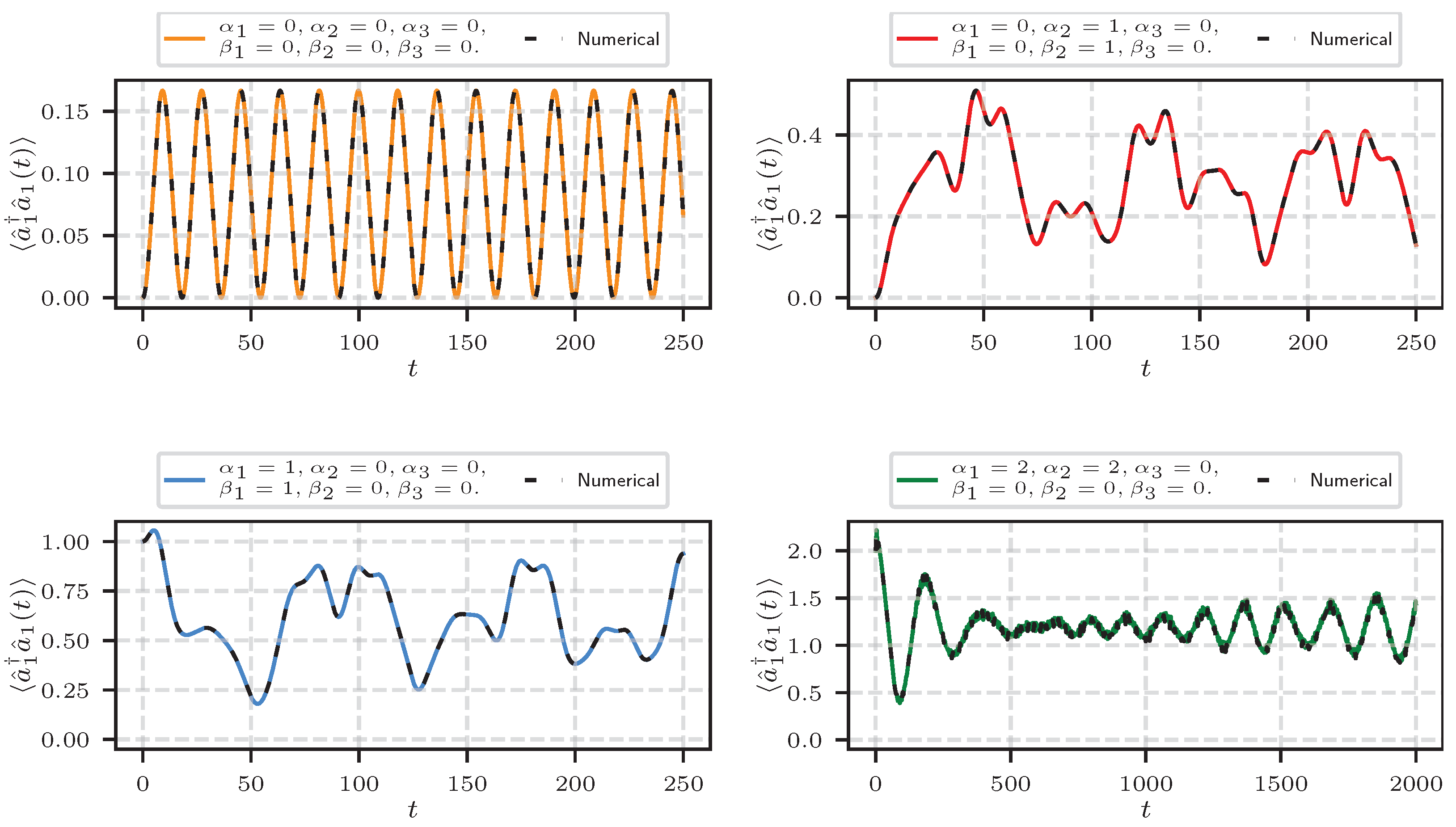
In Figure 3, we show the time evolution of the mean photon number in field 1 for the same parameters as in Figure 2. The solid lines correspond to the analytical results from Equation (34), while the dashed curves represent the numerical solutions of the Schrödinger equation. For vacuum initial states (), Rabi–type oscillations appear, reflecting the exchange of excitations between the atom and the fields. For larger coherent amplitudes, the dynamics become more intricate and exhibit oscillations characteristic of collapse and revival phenomena, in agreement with the behavior of the atomic inversion.
4. Three Quantized Fields Interacting with the Atom
We now consider the case of three quantized fields interacting with a two–level atom. The Hamiltonian describing this system is given by
where the invariants given in Equations (3) and (4) are evaluated for . Similarly to the case, we apply a unitary transformation to move to a new reference frame where all field operators, except those associated with field 1, are eliminated. In this transformed frame, the Schrödinger equation can be solved more straightforwardly. The transformation is defined as
where
Under this transformation, the operators , , and transform according to
From these results, it follows that the invariants transform in the following way
and the operator is transformed as
Finally, the Hamiltonian in the transformed frame takes the form
By setting , the interaction terms involving fields 2 and 3 vanish, and the Hamiltonian reduces to
Through this transformation, we obtain an effective Jaynes–Cummings Hamiltonian for a single field, characterized by an effective coupling constant , together with the free-field Hamiltonian of the remaining quantized modes (2 and 3). Since the evolution operator associated with this Hamiltonian is already known, the evolution of the system in the original frame can be expressed as
with .
4.1. Atomic Inversion and Average Number of Photons
We assume that the system is initially prepared in the state
To determine the system’s evolution, we first apply the operator to the initial state. Before doing so, however, it is convenient to express this operator in factored form. This procedure follows directly by analogy with the case, Equation (12), since the operators involved satisfy the same commutation relations. In particular, because obeys the relation , the same method can be applied here, yielding
where
The last exponential in this expression can be factorized analogously to Equation (48), since the involved operators form a closed algebra under the commutator. Hence, the Wei–Norman theorem[36] can be applied, yielding
where , and
Once the operator has been factorized, and after performing the necessary algebraic manipulations while taking into account that
we obtain the atomic inversion
and the average number of photons
where
with . As observed, when three quantized fields interact with the atom, the Rabi frequency depends on the effective coupling constant , which is larger than the individual atom–field coupling and also greater than that obtained in the two–field case. This enhancement results from the collective action of multiple fields coupling to the same atomic transition. Hence, increasing the number of fields is expected to further enhance the effective coupling and the corresponding oscillation frequency, leading to faster Rabi oscillations. In Figure 4 and Figure 5, we present the temporal evolution of the atomic inversion and the average photon number, respectively. The amplitudes of fields 1 and 2 are chosen to be the same as in the case, while field 3 is initially prepared in the vacuum state. This configuration enables a direct comparison of the system’s dynamics for and , allowing us to identify the specific influence of the additional quantized mode on the atom–field interaction.
As we can see, the dynamics of the atomic inversion resemble those observed in the case where two fields interact with the atom. We observe Rabi oscillations with a higher frequency, as well as collapses and revivals that occur more rapidly than in the case . This behavior indicates that the presence of a third field, even when initially in the vacuum state, modifies the effective coupling between the atom and the radiation modes, leading to a faster exchange of energy between the atomic and field subsystems. In the framework of the Jaynes–Cummings model, it is well known that the revival time of the atomic inversion [6], , depends inversely on the atom–field coupling constant and on the square root of the average photon number. Specifically, it is given by
where g denotes the atom–field coupling constant. This relation, valid in the regime of large coherent-state amplitudes and for long evolution times, shows that an increase in the coupling strength leads to a shorter revival time—consistent with the faster revivals observed when three fields interact with the atom. On the other hand, for the average photon number we observe a similar dynamics to that found in the case . The main difference is that, in the subplot where the collapse and revival phenomena were clearly observed for the case, such behavior becomes much less pronounced when the third field is included. Although a gradual decrease in the oscillations can still be seen—reminiscent of the collapse dynamics—the subsequent rephasing that characterizes the revivals is no longer clearly distinguishable. This suggests that the presence of a third field, even when initially in the vacuum state, alters the redistribution of excitations among the modes, thereby modifying the conditions under which rephasing can occur.
5. Generalization to N Fields
Following the same reasoning employed in the cases and , we now outline the procedure used to generalize these specific scenarios to the case of N quantized fields interacting with a two–level atom. To this end, we apply the corresponding generalized transformation
where
The reason for defining in this manner is that the operator satisfies the commutation relation , which allows us to write
and, together with the fact that the operators resulting from are products of the form , where each satisfies the same commutation relations, they therefore close an algebra under the commutation operation. This property allows us to decouple the exponential by means of the Wei–Norman theorem[36] and, consequently, to factorize the operator so that it can be consistently applied to the initial condition of the system.
Under this transformation, the relevant operators transform as follows
where . From these results, it follows that the invariants transform as
and the operator transforms as
Therefore, the Hamiltonian of the system in the new reference frame is given by
If we set
all fields except field 1 are eliminated, and in this way we obtain the Hamiltonian
which corresponds to a Jaynes–Cummings Hamiltonian with an effective coupling constant , plus the free Hamiltonian of the remaining fields. Since the evolution operator associated with this Hamiltonian is already known, the atomic inversion and the mean photon number can be readily obtained by applying the corresponding operators when the initial state is composed of coherent field states. The main challenge arises from the fact that, as N increases, the number of algebraic manipulations required grows significantly. Moreover, as the number of interacting field modes N increases, the parameter tends toward , leading to an effective coupling constant . This suggests that the atom–field interaction strength, and consequently the Rabi frequency, increase with N, reflecting a collective enhancement effect resulting from the simultaneous coupling of multiple quantized fields to the atom.
6. Conclusions
We have presented a general and unified procedure to describe the dynamics of N degenerate quantized fields resonantly interacting with a single two–level atom within the rotating–wave approximation. By identifying an appropriate set of dynamical invariants, the full evolution operator can be systematically factorized, allowing the multimode Hamiltonian to be mapped; through a suitable unitary transformation, onto an effective Jaynes–Cummings form. A central outcome of this construction is the emergence of an effective coupling constant that increases monotonically with the number of interacting fields. This scaling encapsulates a genuine collective enhancement: as additional degenerate modes participate coherently in the interaction, the atom experiences a progressively stronger effective coupling, reflected in an amplified Rabi frequency and a more pronounced dynamical response.
The explicit implementations for the cases of two and three quantized fields illustrate the structure and transparency of the general method. These examples reveal how the invariants, unitary reduction, and effective Hamiltonian emerge in a natural and hierarchical fashion, providing a clear pathway for extending the analysis to an arbitrary number N of degenerate modes. For initially coherent field states and an atom prepared in a superposition of its internal levels, we computed the atomic inversion and mean photon number, observing vacuum Rabi oscillations as well as the characteristic collapse–revival phenomenon. Overall, the procedure developed here not only generalizes the Jaynes–Cummings model to a multimode scenario while preserving its essential physical content, but also demonstrates how the collective increase in the effective coupling strength enriches the dynamical behavior. This framework provides a robust foundation for exploring more elaborate multimode quantum-optical configurations and for analyzing cooperative atom–field effects in increasingly complex quantum architectures.
Author Contributions
All authors contributed equally to each of the requirements necessary for the elaboration of this manuscript. All authors have read and agreed to the published version of the manuscript.
Funding
This research received no external funding.
Data Availability Statement
No new data were created or analyzed in this study.
Acknowledgments
Marco Antonio García-Márquez thanks the Secretariat of Science, Humanities, Technology and Innovation (SECIHTI) and the National Institute of Astrophysics, Optics and Electronics (INAOE) for the doctoral scholarship.
Conflicts of Interest
The authors declare no conflict of interest.
References
- Rabi, I.I. Space Quantization in a Gyrating Magnetic Field. Phys. Rev. 1937, 51, 652–654. [Google Scholar] [CrossRef]
- Braak, D. Integrability of the Rabi Model. Phys. Rev. Lett. 2011, 107, 100401. [Google Scholar] [CrossRef] [PubMed]
- Jaynes, E.; Cummings, F. Comparison of quantum and semiclassical radiation theories with application to the beam maser. Proceedings of the IEEE 1963, 51, 89–109. [Google Scholar] [CrossRef]
- Shore, B.W.; Knight, P.L. The jaynes-cummings model. Journal of Modern Optics 1993, 40, 1195–1238. [Google Scholar] [CrossRef]
- Larson, J.; Mavrogordatos, T. The Jaynes–Cummings Model and Its Descendants; 2053-2563, IOP Publishing, 2021. [CrossRef]
- Eberly, J.H.; Narozhny, N.B.; Sanchez-Mondragon, J.J. Periodic Spontaneous Collapse and Revival in a Simple Quantum Model. Phys. Rev. Lett. 1980, 44, 1323–1326. [Google Scholar] [CrossRef]
- Narozhny, N.B.; Sanchez-Mondragon, J.J.; Eberly, J.H. Coherence versus incoherence: Collapse and revival in a simple quantum model. Phys. Rev. A 1981, 23, 236–247. [Google Scholar] [CrossRef]
- Meystre, P.; Zubairy, M. Squeezed states in the Jaynes-Cummings model. Physics Letters A 1982, 89, 390–392. [Google Scholar] [CrossRef]
- Guo, G.C.; Zheng, S.B. Generation of Schrödinger cat states via the Jaynes-Cummings model with large detuning. Physics Letters A 1996, 223, 332–336. [Google Scholar] [CrossRef]
- Anaya-Contreras, J.A.; Ramos-Prieto, I.; Zúñiga-Segundo, A.; Moya-Cessa, H.M. The anisotropic quantum Rabi model with diamagnetic term. Frontiers in Physics 2025, Volume 13 - 2025. [Google Scholar] [CrossRef]
- Campos-Uscanga, A.; Rodríguez, E.B.; Martínez, E.P.; Bastarrachea-Magnani, M.A. Magic States in the Asymmetric Quantum Rabi Model. arXiv, 2025; arXiv:quant-ph/2508.00765. [Google Scholar]
- Asbóth, J.K.; Domokos, P.; Ritsch, H. Correlated motion of two atoms trapped in a single-mode cavity field. Phys. Rev. A 2004, 70, 013414. [Google Scholar] [CrossRef]
- Roversi, J.A.; Vidiella-Barranco, A.; Moya-Cessa, H. Dynamics of two atoms coupled to a cavity field. Modern Physics Letters B 2003, 17, 219–224. [Google Scholar] [CrossRef]
- Dicke, R.H. Coherence in Spontaneous Radiation Processes. Phys. Rev. 1954, 93, 99–110. [Google Scholar] [CrossRef]
- Braak, D. Solution of the Dicke model for N = 3. Journal of Physics B: Atomic, Molecular and Optical Physics 2013, 46, 224007. [Google Scholar] [CrossRef]
- Tavis, M.; Cummings, F.W. Exact Solution for an N-Molecule—Radiation-Field Hamiltonian. Phys. Rev. 1968, 170, 379–384. [Google Scholar] [CrossRef]
- Abdel-Hafez, A.M.; Obada, A.S.F.; Ahmad, M.M.A. N-level atom and (N-1) modes: an exactly solvable model with detuning and multiphotons. Journal of Physics A: Mathematical and General 1987, 20, L359. [Google Scholar] [CrossRef]
- Kochetov, E. A generalized N-level single-mode Jaynes-Cummings model. Physica A: Statistical Mechanics and its Applications 1988, 150, 280–292. [Google Scholar] [CrossRef]
- Bužek, V. N-level Atom Interacting with Single-mode Radiation Field: An Exactly Solvable Model with Multiphoton Transitions and Intensity-dependent Coupling. Journal of Modern Optics 1990, 37, 1033–1053. [Google Scholar] [CrossRef]
- Kumar, N.; Chatterjee, A. Nonclassicality in a dispersive atom–cavity field interaction in presence of an external driving field. International Journal of Modern Physics B 2024, 38, 2450415. [Google Scholar] [CrossRef]
- Vidiella-Barranco, A.; Magalhães de Castro, A.S.; Sergi, A.; Roversi, J.A.; Messina, A.; Migliore, A. Analytical Solutions of the Driven Time-Dependent Jaynes–Cummings Model. Annalen der Physik 2025, 537, e00148. [Google Scholar] [CrossRef]
- Bocanegra-Garay, I.A.; Hernández-Sánchez, L.; Ramos-Prieto, I.; Soto-Eguibar, F.; Moya-Cessa, H.M. Invariant approach to the driven Jaynes-Cummings model. SciPost Physics 2024, 16, 007. [Google Scholar] [CrossRef]
- Buck, B.; Sukumar, C. Exactly soluble model of atom-phonon coupling showing periodic decay and revival. Physics Letters A 1981, 81, 132–135. [Google Scholar] [CrossRef]
- Sukumar, C.; Buck, B. Multi-phonon generalisation of the Jaynes-Cummings model. Physics Letters A 1981, 83, 211–213. [Google Scholar] [CrossRef]
- Singh, S. Field statistics in some generalized Jaynes-Cummings models. Phys. Rev. A 1982, 25, 3206–3216. [Google Scholar] [CrossRef]
- Papadopoulos, G.J. Energetics of radiation and a two-level atom in an ideal resonant cavity. Phys. Rev. A 1988, 37, 2482–2487. [Google Scholar] [CrossRef] [PubMed]
- Abdalla, M.; Ahmed, M.; Obada, A.S. Multimode and multiphoton processes in a non-linear Jaynes-Cummings model. Physica A: Statistical Mechanics and its Applications 1991, 170, 393–414. [Google Scholar] [CrossRef]
- Wildfeuer, C.; Schiller, D.H. Generation of entangled N-photon states in a two-mode Jaynes-Cummings model. Phys. Rev. A 2003, 67, 053801. [Google Scholar] [CrossRef]
- Abdalla, M.S.; Ahmed, M.M.A.; Obada, A.S.F. Some statistical properties of the interaction between a two-level atom and three field modes. Laser Physics 2015, 25, 065204. [Google Scholar] [CrossRef]
- Seke, J. Extended Jaynes–Cummings model. J. Opt. Soc. Am. B 1985, 2, 968–970. [Google Scholar] [CrossRef]
- Dutra, S.M.; Knight, P.L.; Moya-Cessa, H. Discriminating field mixtures from macroscopic superpositions. Phys. Rev. A 1993, 48, 3168. [Google Scholar] [CrossRef]
- Benivegna, G. Quantum effects in the transient dynamics of a many mode Jaynes-Cummings model. Journal of Modern Optics 1996, 43, 1589–1601. [Google Scholar] [CrossRef]
- Larson, J. Scheme for generating entangled states of two field modes in a cavity. Journal of Modern Optics 2006, 53, 1867–1877. [Google Scholar] [CrossRef]
- Benivegna, G.; Messina, A. New Quantum Effects in the Dynamics of a Two-mode Field Coupled to a Two-level Atom. Journal of Modern Optics 1994, 41, 907–925. [Google Scholar] [CrossRef]
- Sakurai, J.J.; Napolitano, J. Modern Quantum Mechanics, 3 ed.; Cambridge University Press, 2020.
- Wei, J.; Norman, E. On global representations of the solutions of linear differential equations as a product of exponentials. Proceedings of the American Mathematical Society 1964, 15, 327–334. [Google Scholar] [CrossRef]
- Gerry, C.; Knight, P. Introductory Quantum Optics; Cambridge University Press, 2004.
Figure 1.
A two-level atom interacting with N quantized cavity field modes of equal frequency via identical Jaynes–Cummings couplings. The modes are mutually uncoupled and interact only through the atom.
Figure 1.
A two-level atom interacting with N quantized cavity field modes of equal frequency via identical Jaynes–Cummings couplings. The modes are mutually uncoupled and interact only through the atom.
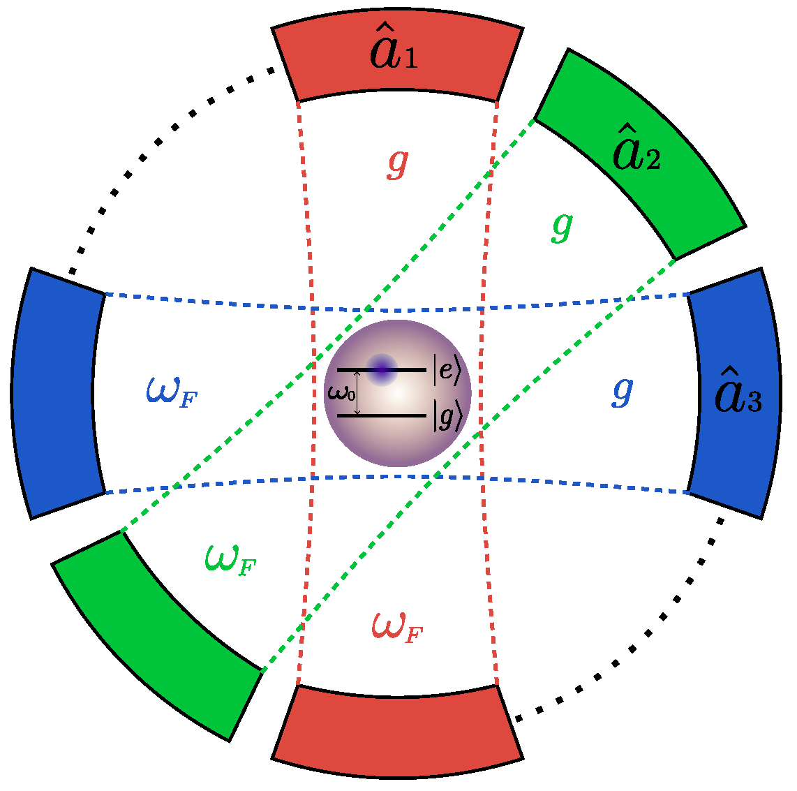
Figure 2.
Time evolution of the atomic inversion for various amplitudes of the initial coherent field states. The parameters used are and . Solid colored lines denote the analytical results, and dashed curves correspond to the numerical simulations.
Figure 2.
Time evolution of the atomic inversion for various amplitudes of the initial coherent field states. The parameters used are and . Solid colored lines denote the analytical results, and dashed curves correspond to the numerical simulations.
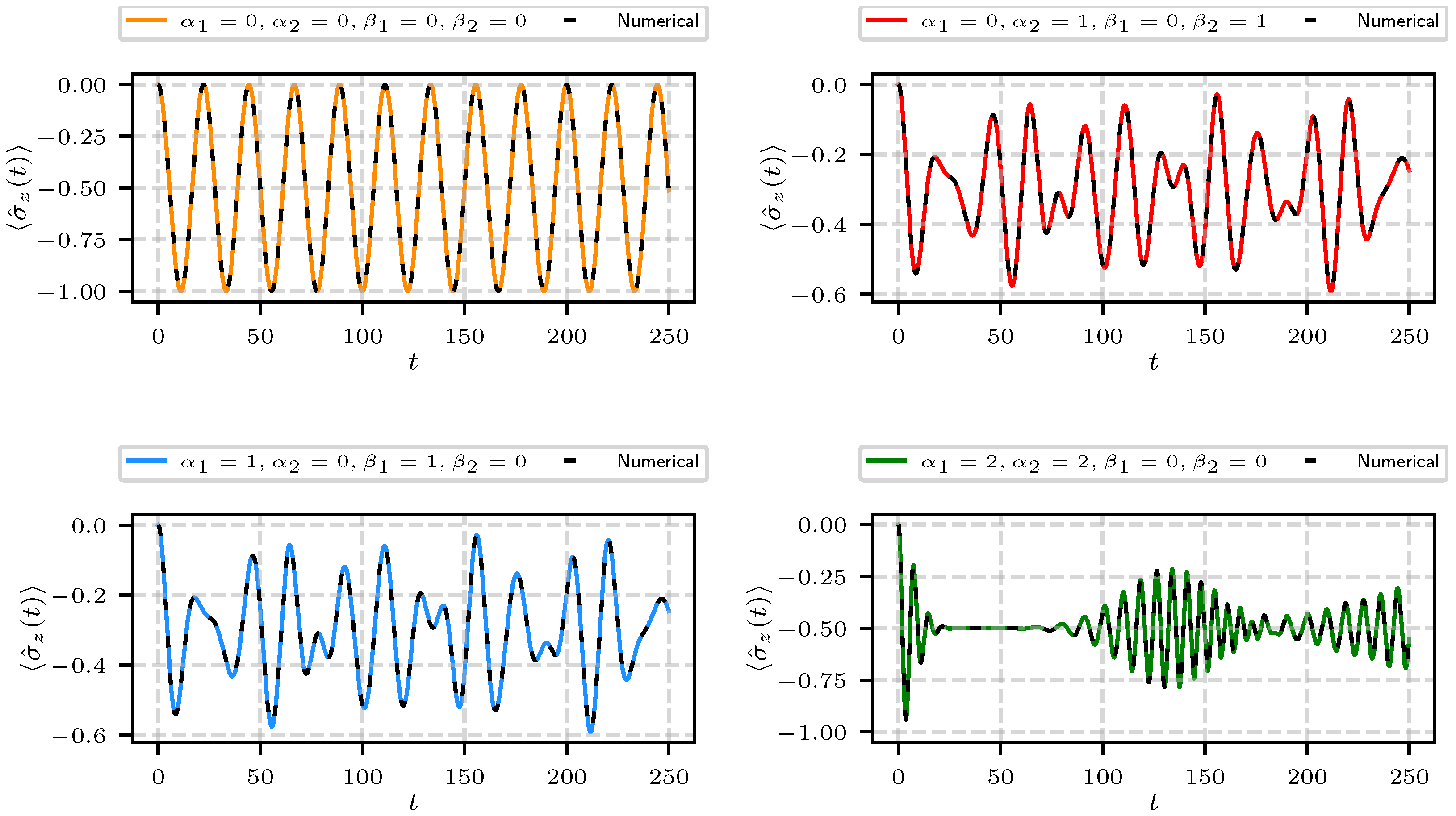
Figure 3.
Time evolution of the mean photon number in field 1 for various amplitudes of the initial coherent field states. The parameters used are and . Solid colored lines denote the analytical results, while dashed curves correspond to the numerical simulations.
Figure 3.
Time evolution of the mean photon number in field 1 for various amplitudes of the initial coherent field states. The parameters used are and . Solid colored lines denote the analytical results, while dashed curves correspond to the numerical simulations.
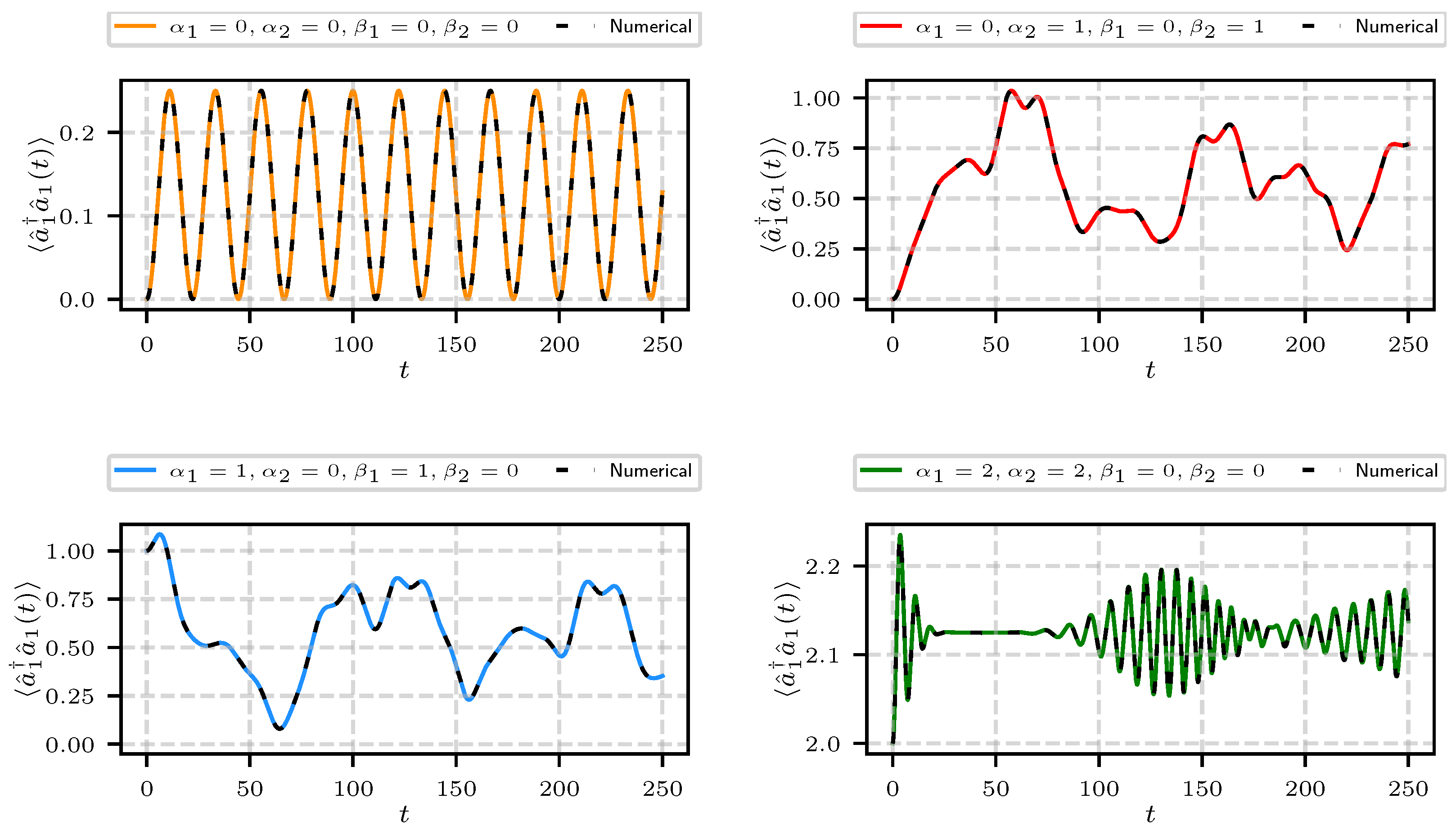
Figure 4.
Time evolution of the atomic inversion for the case of three quantized fields interacting with a two-level atom, for various amplitudes of the initial coherent field states. The parameters used are and . Solid colored lines denote the analytical results, and dashed curves correspond to the numerical simulations.
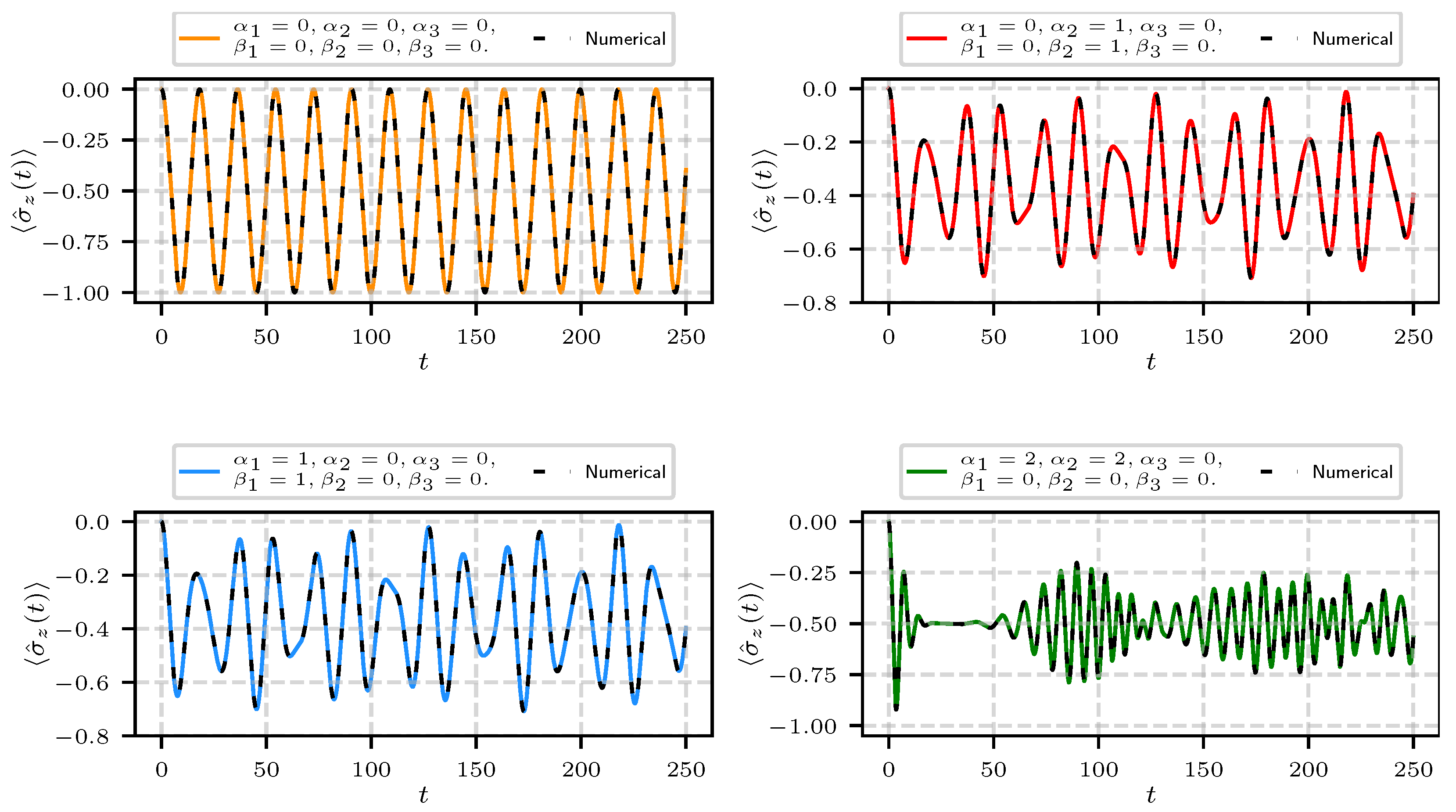
Figure 5.
Time evolution of the average photon number in field 1 for the case of three quantized fields interacting with a two-level atom, for various amplitudes of the initial coherent field states. The parameters used are and . Solid colored lines denote the analytical results, and dashed curves correspond to the numerical simulations.
Disclaimer/Publisher’s Note: The statements, opinions and data contained in all publications are solely those of the individual author(s) and contributor(s) and not of MDPI and/or the editor(s). MDPI and/or the editor(s) disclaim responsibility for any injury to people or property resulting from any ideas, methods, instructions or products referred to in the content. |
© 2025 by the authors. Licensee MDPI, Basel, Switzerland. This article is an open access article distributed under the terms and conditions of the Creative Commons Attribution (CC BY) license (http://creativecommons.org/licenses/by/4.0/).
Copyright: This open access article is published under a Creative Commons CC BY 4.0 license, which permit the free download, distribution, and reuse, provided that the author and preprint are cited in any reuse.


