Submitted:
27 November 2025
Posted:
28 November 2025
You are already at the latest version
Abstract
Single-phase-to-ground faults occur frequently in distribution networks, and traditional localization methods have limitations such as insufficient feature extraction and poor topological adaptability. This paper proposes a two-stage localization method integrating the node classification matrix and the improved binary particle swarm optimization (IBPSO) algorithm: the node classification matrix achieves rapid initial localization, while IBPSO performs error correction. Simulation verification based on the IEEE 33-bus model shows that the method achieves a localization accuracy of 96%, which is 19% higher than that of the node classification matrix and 2% higher than that of IBPSO. It still maintains an accuracy of over 95% under scenarios of 1-3 node distortions, topological switching, and 5000Ω high-impedance faults, and is compatible with existing FTU (Feeder Terminal Unit) devices. This method effectively balances localization speed and robustness, providing a reliable solution for the rapid isolation of distribution network faults.
Keywords:
distribution network
; fault location
; improved binary particle swarm algorithm
; node classification matrix
; topology adaptability
1. Introduction
Distribution networks serve as the hub connecting transmission systems and power users, with their safe and stable operation directly impacting national economic development and residents' quality of life. Statistics show that single-phase-to-ground faults account for as high as 70%-80% of distribution network faults [1]. This type of fault is characterized by small ground current and transient symmetry of system voltage, and can theoretically operate for a short time. However, overvoltage in non-fault phases is prone to causing arc discharge, accelerating the insulation aging of equipment, and even expanding into phase-to-phase short circuits [2]. With the large-scale integration of distributed generation (photovoltaic, energy storage), the dynamic changes of distribution network topology have intensified. Traditional localization methods are facing three major challenges: difficulty in identifying high-impedance faults, sensitivity to node information distortion, and poor topological adaptability. Thus, a more reliable localization scheme is urgently needed.
Existing distribution network fault localization technologies can be divided into four categories, but all have significant drawbacks and struggle to meet the requirements of complex operating conditions. Matrix-based methods These methods construct topological matrices and fault information matrices based on graph theory [3], quickly matching fault sections through matrix operations with high computational efficiency . However, such methods have low localization accuracy for terminal sections [4] and rely on the integrity of FTU data. Intelligent optimization-based methods They transform the localization problem into a 0-1 integer programming problem. For example, the traditional BPSO algorithm searches for the optimal solution through particle iteration, with robustness superior to matrix-based methods. Nevertheless, traditional BPSO is prone to falling into local optima and fails to utilize topological prior information. Full-space search results in more than 9 iterations and a localization time exceeding 200ms [5], making it difficult to meet real-time requirements. Signal analysis-based methods These methods extract fault features through zero-sequence current/voltage [6], featuring strong specificity. However, they depend on the density of measurement nodes, require re-calibration of feature thresholds when topology changes, and have poor adaptability.Deep learning-based methods Emerging models such as CNN and LSTM in recent years improve accuracy through data-driven approaches. But they require massive fault samples and suffer from poor model interpretability . Meanwhile, they are sensitive to output fluctuations of distributed generation, with accuracy decreasing by 15% when sample distribution shifts [16], leading to great difficulties in engineering application.
To address the aforementioned issues, the principles of the node classification matrix algorithm and the improved binary particle swarm optimization (IBPSO) algorithm are analyzed first. A fault localization workflow is then proposed, followed by the introduction of a novel localization method that integrates the node classification matrix with the improved binary particle swarm.This approach demonstrates significant advantages over traditional algorithms in terms of localization speed, fault tolerance, and global optimization capability.
2. Fault Section Location Algorithm Based on Node Classification Matrix
2.1. Algorithm Principles
Traditional matrix-based algorithms struggle to pinpoint faults in terminal line segments. Furthermore, complex matrix calculations are required for their normal operation. This makes computations cumbersome for distribution networks with multiple nodes and complex topology. To address these issues, a fault segment localization method based on a node classification matrix is proposed.This method constructs a network topology matrix describing the distribution network topology based on graph theory, thereby generating a fault path matrix and a fault determination matrix. When a fault occurs, the upstream node among the nodes at both ends of the faulted section is the faulty node, while the downstream node is the healthy node. The section between them constitutes the fault path. By retrieving the corresponding matrix element in the fault determination matrix for this path, rapid and accurate fault section localization is achieved.
Assuming there are N nodes on the line, the line's topological structure can be represented by an Nth-order matrix, defined as shown in Equation(1):
Where: D represents the network topology matrix, and di.j denotes the element in the i row and j column of D. When nodes i and j are electrically connected on a line and current flows from i to j, di.j=1. When there is no electrical connection between nodes i and j or current flows from j to i, di.j=0.
The node classification matrix S is a row matrix of size 1×N, where its elements are determined by node types. During single-phase ground faults in distribution networks, node states fall into only two categories: faulty nodes and healthy nodes. Therefore, node classification results can be expressed using discrete integer values of 0 or 1. If calculations indicate that the i node is the fault node upstream of the fault, it is denoted as si=1; otherwise, it is denoted as 0. The node classification matrix S and the si formula are shown in Equations (2) and (3):
The fault path matrix B is an N×N matrix, defined by Equation(4), representing the upstream paths of fault points. It is jointly determined by the network topology matrix and node classification results. The element bi.j in B corresponds to row i and column j. If the segment between node i and node j has a topological connection and lies on the fault upstream path, bi.j=1; otherwise, the segment is a non-fault path, denoted as bi.j=0. The specific generation steps are as follows: Query the element si in the node classification matrix S. When si=0, node is a healthy node downstream of the fault, and all connected downstream segments are non-fault paths. Therefore, set all entries in row i of the topology matrix D to 0. When si=1, the node is a faulty node upstream of the fault. Query the elements in row i of . If only one element di.j=1 exists in this row, it proves that faulty node i is connected to only one segment, and the line segment between nodes i and j must be the fault path, and di.j=1. If multiple elements in the row are 1, this indicates the node is connected to multiple segments. Compare the zero-sequence current transient energy matrices at the start of each segment; the largest value corresponds to the fault section, and di.j=1, while the others are set to zero.
The fault diagnosis matrix G can simultaneously represent both the node classification results and the fault path matrix. The element gi.j in G, located at row i and column j, is obtained by filling the main diagonal of the fault path matrix B with values from the node classification matrix S. The expression is shown in Equation(5):
2.2. Fault Section Identification Process
Precise fault section localization can be achieved by analyzing the state characteristics of nodes at both ends of the fault path. Specifically, for nodes i and j at the two ends of the fault section, where node i (upstream) is the faulty node and node j(downstream) is the healthy node, and the topology between nodes i and j is in a connected state and constitutes the fault path, the following fault section identification process is established based on this characteristic:
First, scan the elements along the main diagonal of the matrix to locate the first non-zero element gi.i. The node corresponding to this element, i is identified as the initial fault node. Next, check whether any other non-zero elements gj.j=1 exist in the row containing the fault node i. If present, this confirms an active electrical connection exists between nodes i and j, forming the fault current path. Further validate node j status. If gj.j=0, node j is healthy, confirming the fault section lies between nodes i and j. If gj.j=1, continue searching downstream nodes.
3. Improved Binary Particle Swarm Algorithm for Fault Section Localization
3.1. Algorithm Principles
The node classification information and distribution network topology information described earlier are both represented by “1” and “0”. Therefore, the section localization problem can be viewed as an optimization problem with 0-1 discrete constraints, making it suitable for modeling and solving using the Binary Particle Swarm Optimization (BPSO) algorithm. The traditional BPSO algorithm maps the velocity vector to the probability of the position taking the value 1 via a Sigmoid function. Its position update formulas are given as Equations (6) and (7).
However, the traditional BPSO algorithm has difficulties in searching for optimal solutions over a large range and is highly prone to falling into local optima. To address this issue, the traditional BPSO algorithm is improved by introducing a genetic mutation mechanism and a dynamic inertia weight strategy.This approach assigns particles with a certain probability to the locally optimal and globally optimal particles within the particle swarm, while mutating other particles with a specific probability. During the later stages of iteration, when particles begin to cluster locally, methods such as selective crossover are employed to enhance diversity among particles. This facilitates the search for superior solutions across a broader domain. The improved iteration process is outlined as follows:
Where, Equation(8) represents the genetic component, Equation(9) represents the mutation component, and bf denotes the mutation factor during the iteration process.
Following the traditional algorithm's method of setting inertial weights to decrease linearly, the parameters for the coefficient of variation are set as follows:
Where,t represents the current iteration count, T denotes the maximum iteration count, bfmax signifies the maximum mutation factor, and bfmin indicates the minimum mutation factor.
3.2. Fault Section Location Process
Let L(i)(i=1,2,3,…,m) denote the status of the i section. When a section fails, set L(i)=1; when section i is not in a fault state, set L(i)=0. The specific constraints are shown in Equation (11):
The node classification status code N(i) is consistent with the definition of the node classification matrix described above. If node i is a faulty node, then N(i)=1 ; if node i is a healthy node, then N(i)=0. The formula is as follows:
Next, to match the classification status of each node based on the section status code—that is, to determine the expected value for partitioning the node classification results—a target function must be further constructed. As noted above, when a single-phase ground fault occurs in a section, the node upstream of the fault is the faulty node, while the downstream node remains healthy. Based on this, the target function relationship is established as follows:
Where: represents the objective function for node i, Lx denotes the state of the downstream segment of node i, and indicates the logical OR operation. For the terminal node of a line, which is necessarily downstream of a fault, the objective function is directly set to 0.
The principle of fault section localization based on the IBPSO algorithm is as follows: Compare the difference between the expected classification information of a node obtained through the objective function calculation and its actual classification information. The smaller the difference, the more reasonable the interpretation of the fault information becomes, and the better the fault section matches the actual fault section. The fitness function is shown in Equation (14):
In the formula, Ij represents the expected classification information of node j determined by the objective function, Ij denotes the actual classification information of node j , N is the total number of nodes, M is the total number of segments, and ω2 is the penalty coefficient for function misclassification, typically set to ω2=0.5. The solution corresponding to the algorithm's optimal fitness is the state assigned to each segment. The segment marked as “1” in the segment status code corresponding to the minimum fitness value is the faulty segment.
4. Location Algorithm Based on Integration of Node Classification Matrix and Improved Binary Particle Swarm Optimization
The integration of the node classification matrix and the Improved Binary Particle Swarm Optimization (IBPSO) algorithm is not a simple combination of the two methods, but rather a collaborative framework constructed based on their complementary characteristics and the inherent patterns of distribution network fault location.The section localization method based on the node classification matrix has the advantages of clear operations and simple implementation. However, when node classification information is distorted, this method is prone to misjudgment, resulting in the overlap between true fault sections and false fault sections. In contrast, the fault location method based on the IBPSO algorithm, despite its higher computational complexity, can effectively mitigate the impact of node classification distortion. Accurate identification of fault sections is still achievable even under such abnormal conditions.
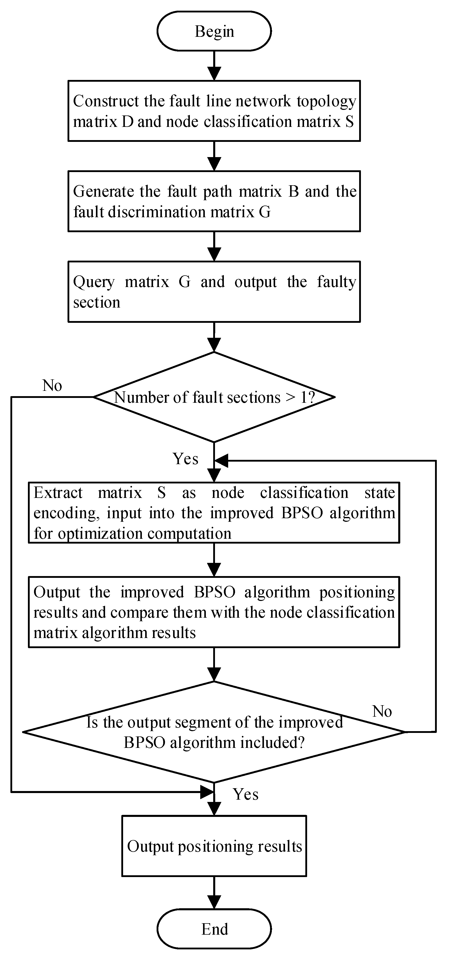
The rapidity of the node classification matrix compensates for the insufficiency in real-time performance of BPSO, and the robustness of BPSO addresses the matrix's sensitivity to information distortion. The two thus form the theoretical basis for efficiency-accuracy complementarity.Therefore, this section integrates the strengths of both approaches, proposing a hybrid location algorithm combining the node classification matrix with the IBPSO to enhance the reliability of location results. The core concept of this algorithm is as follows: First, perform rapid initial localization using the node classification matrix algorithm. If its output indicates multiple faults, initiate the IBPSO algorithm for secondary localization and error correction. Then, verify the secondary localization results against the output of the node classification matrix algorithm. If the fault section identified by the former is contained within the latter's set of multiple segments, it indicates that false fault sections have been successfully eliminated. Finally, the localization results are output.
Figure 1.
Flow chart of fault section location method.
5. Simulation Verification and Analysis
Construct the simulation model according to Figure 2, where nodes are numbered 1-33 and segments are labeled L1-L32. Set the particle dimension to 32, the number of particles to 20, and the maximum iteration count to 50 (convergence is permitted before iteration termination). The learning factors are c1=c2=2.1,the particle dimension is d=7 and the maximum velocity is Vmax=4 Initial inertia weight coefficient ω1=0.9 maximum mutation factor bfmax=0.2.
5.1. Fault Section Location Under Typical Conditions
L28 was set to experience a single-phase ground fault with an initial fault angle of 90°and a transition resistance of 10Ω. No distortion was observed in the node classification results. At this point, the node classification matrix S is [1 1 1 1 1 1 0 0 0 0 0 0 0 0 0 0 0 0 0 0 0 0 0 0 0 1 1 1 0 0 0 0 0], and the fault path is segment L1, L2, L3, L4, L5, L25, L26, L27, and L28. The fault determination matrix G is presented in Figure 3. Querying reveals the fault occurred between nodes 28 and 29, thus correctly outputting the fault section as L28.
Simulation results with altered fault conditions and locations are shown in the table below:
As shown in Table 1, when node classification information remains unchanged, altering other conditions does not affect the correct output of segment localization results. Furthermore, localization can be achieved solely through the first-step algorithm based on the node classification matrix, without requiring an IBPSO algorithm supplemented by iterative operations. The results are reliable, and the localization process is simple and fast.
5.2. Fault Section Location Based on IBPSO Algorithm
A single-phase ground fault was set in section L8 with an initial fault angle of 90° and a transition resistance of 10Ω. Meanwhile, a single-point distortion was introduced in the node classification results: node 3 (upstream of the fault) changed from 1 to 0. At this point, the node classification matrix S is [1 1 0 1 1 1 1 1 0 0 0 0 0 0 0 0 0 0 0 0 0 0 0 0 0 0 0 0 0 0 0 0 0], and the fault determination matrix G is shown in Figure 4:
Upon inquiry, the output fault sections are L2 and L8. Due to multiple fault sections being output, the enhanced BPSO algorithm is initiated. The node classification matrix is extracted as node classification information encoding input into the enhanced BPSO algorithm for optimization computation. The output results are: [0 0 0 0 0 0 0 1 0 0 0 0 0 0 0 0 0 0 0 0 0 0 0 0 0 0 0 0 0 0 0 0 0], confirming fault section L8. The fitness curve evolution is shown in Figure 5. The segment output by the IBPSO algorithm matches the segment output by the node classification matrix algorithm, confirming that segment L2 is a false fault section. The true fault section L8 is thus identified.
Secondly, multi-point distortion simulation verification was conducted by changing the fault section to L31. Distortion nodes were set at upstream nodes significantly affecting the location results: nodes 3, 4, and 27. All three nodes changed from 1 to 0. At this point, the node classification matrix is [1 1 0 0 1 1 0 0 0 0 0 0 0 0 0 0 0 0 0 0 0 0 0 0 0 1 0 1 1 1 1 0 0]. Due to space constraints, the specific form of the fault determination matrix is not shown here. The matrix query results indicate the fault sections as L2, L26, L31. Secondary localization was performed using an IBPSO algorithm, with the convergence curve shown in Figure 6. The output result is [0 0 0 0 0 0 0 0 0 0 0 0 0 0 0 0 0 0 0 0 0 0 0 0 0 0 0 0 0 0 1 0 0], confirming fault section L31. After result verification, the final correct output was segment L31.
Multiple simulations were conducted by altering the fault location, node distortion position, and number of nodes. The results are shown in Table 2.
The simulation results demonstrate that when single-point or multi-point distortion occurs in node classification information, the node classification matrix algorithm may initially identify multiple fault sections. However, after error correction via the IBPSO algorithm, accurate fault location can still be achieved. The method presented in this chapter exhibits excellent fault tolerance and high accuracy.
5.3. Fault Section Location in Distribution Networks with Topology Changes
During actual operation of distribution networks, frequent switching operations can alter the network topology. Consider the distribution network model shown in Figure 2: if the section between nodes 7 and 8 is disconnected and the section between nodes 18 and 22 is connected, simulating with these modified fault conditions and locations yields the fault location results presented in Table 3.
As shown in Table 3, the proposed method can still achieve accurate fault section location even when the distribution network topology changes.
5.4. Verification of Performance Advantages of Fusion Algorithms
In the distribution network model shown in Figure 5, simulations were conducted using three algorithms: the node classification matrix algorithm, the IBPSO algorithm, and the proposed fusion algorithm (integrating the node classification matrix with the IBPSO). The advantages of the fusion algorithm in location accuracy and speed were then compared.Assuming a fault occurs in section L12, with 100 simulation runs conducted. For each run, the number of randomly distorted nodes was set between 0 and 3. The positioning performance of each algorithm is summarized in the table below:
As shown in Table 4, the node classification matrix-based algorithm demonstrates a significant advantage in computational speed, completing fault section localization within 1.32ms. However, it is highly prone to localization errors when node classification information is distorted, achieving only 77% localization accuracy. The IBPSO algorithm demonstrates strong fault-tolerant performance and high accuracy, but suffers from slower localization speed due to its higher iteration count, averaging 202.5ms. The proposed fault localization model in this chapter, which integrates the node classification matrix with the IBPSO algorithm, achieves an average processing time of 16.1ms and a correctness rate of 96%. By combining the strengths of both approaches, it offers superior performance with balanced accuracy and speed advantages.
To further validate the advantages of the proposed hybrid algorithm over the IBPSO algorithm in terms of computational speed, Figure 7 presents a comparison of the minimum number of iterations achieved by each method at the conclusion of each simulation run across 100 simulations.
In Figure 10, Algorithm 1 refers to the IBPSO algorithm, while Algorithm 2 denotes the fusion algorithm. As shown by the curves, the proposed fusion algorithm can complete segment localization without iterations in most cases. Its average iteration count is significantly lower than that of the single IBPSO algorithm, demonstrating a marked advantage in localization speed.
To further validate the accuracy advantages of the fusion algorithm over the single-node classification matrix algorithm and mitigate the randomness associated with single-fault locations, simulations were conducted with fault sections set to L3, L27, and L17. Random node distortions were introduced with distortion counts of 1 and 3. Each fault condition was simulated 100 times. The positioning accuracy rates for the fusion algorithm and the single-node classification matrix algorithm are summarized in the table below:
Analysis of Table 5 reveals that as the number of node distortions increases, the localization accuracy of the node classification matrix algorithm decreases. In contrast, the fusion algorithm consistently maintains high accuracy under varying fault locations and node distortion counts, demonstrating superior fault tolerance performance.
6. Conclusion
This paper proposes a fault section localization method for distribution networks that integrates a node classification matrix with an improved binary particle swarm algorithm. The main conclusions are as follows:
(1)This paper proposes a dual-dimension-driven method for constructing the node classification matrix, which integrates topological features and node states. It addresses the problems of traditional matrix-based algorithms, namely the difficulty in locating terminal sections and cumbersome computation under complex topologies.
(2)This paper designs a synergistically improved BPSO algorithm integrating genetic mutation and dynamic inertia weight, which overcomes the shortcomings of traditional BPSO—weak global search capability and proneness to local optima. It can still stably converge to the optimal solution in scenarios with node information distortion, providing a reliable optimization tool for error correction.
(3)This paper proposes a two-stage fusion architecture with both rapidity and robustness, and verifies the algorithm's engineering applicability under scenarios of node distortion, topological changes, and high-impedance faults.
This paper still has aspects to be improved: first, it has not fully considered the impact of output fluctuations of distributed generation (photovoltaic /energy storage) on node classification results; second, in large-scale distribution networks such as the IEEE 123-node system, the computational efficiency of the algorithm needs further optimization.
Abbreviations
The following abbreviations are used in this manuscript:
| IBPSO | Improved binary particle swarm optimization |
| FTU | Feeder Terminal Unit |
| BPSO | Binary Particle Swarm Optimization |
References
- Jinian,P.;Juan,L.;Xiuru,W.et.al. Distribution network fault self-healing scheme based on network partition and flexible resource aggregation.Frontiers in Energy Research.2025;pp.131538033-1538033.
- Pirmani,K.S.; Fernando,P.S.W.;Mahmud,A.M. Single line-to-ground fault current analysis for resonant grounded power distribution networks in bushfire prone areas.Electric Power Systems Research.2024;pp.237110883-110883.
- Wang,C.;Feng,L.;Hou,S.et.al. A Method for Single-Phase Ground Fault Section Location in Distribution Networks Based on Improved Empirical Wavelet Transform and Graph Isomorphic Networks.Information.2024,15(10),650-650.
- Seyed.;Hossein.;Mortazavi,et.al. An analytical fault location method based on minimum number of installed PMUs. International Transactions on Electrical Energy Systems. 2015,26,253-273.
- Wang,H.;Huang,C.;Yu,H,et.al. Method for fault location in a low-resistance grounded distribution network based on multi-source information fusion. International Journal of Electrical Power & Energy Systems. 2021,125: 106384.
- Lan,J.;Zhu,G.;Qin,F.et.al. A fault section location method based on zero mode current traveling wave for high-resistance grounding of distribution network.2020 Asia Energy and Electrical Engineering Symposium (AEEES). Chengdu, China,IEEE, 2020;pp.602-606.
- Degano;Iván,L.;Fiaschetti,L.;Lotito,P.A. Location of faults based on deep learning with feature selection for meter placement in distribution power grids. International Journal of Emerging Electric Power Systems. 2024, 25(5),657-666.
- Paulo,A.;Madson,C.Fault location approach for distribution systems based on modern monitoring infrastructure. IET Generation, Transmission & Distribution. 2018, 12(1),94-103.
- Song,G.;Ma,Z.;Li,G.et.al. Phase current fault component based single-phase earth fault segment location in non-solidly earthed distribution networks. International Transactions on Electrical Energy Systems.2015, 25(11),2713-2730.
- Cai,B.;Huang,L.;Xie,M.Bayesian networks in fault diagnosis. IEEE Transactions on Industrial Informatics.2017, 13(5),2227-2240.
- Wang,C.;Feng, Hou,S.et.al. A method for single-phase ground fault section location in distribution networks based on improved empirical wavelet transform and graph isomorphic networks. Information. 2024, 15(10),650.
- Jangdoost,A.;Keypour,R.;Golmohamadi,H. Optimization of distribution network reconfiguration by a novel RCA integrated with genetic algorithm. Energy Systems. 2020, 12(3),1-33.
- Xu,G.;Guo,Z. Resilience enhancement of distribution networks based on demand response under extreme scenarios. IET Renewable Power Generation. 2024, 18(1),48-59.
- Zhang,S.;Li,L.; Zhao,H.et.al. The optimization strategy of loop closing operation in self-healing distribution network. Applied Mechanics and Materials. 2014, 519-520,1375-1378.
- Shen,Q. A novel method of fault line selection in low current grounding system using multi-criteria information integrated. Electric Power Systems Research,2022, 209,108010.
- Yang,D.; Lu,B.; Lu,H. High-resistance grounding fault detection and line selection in resonant grounding distribution network. Electronics.2023, 12(19),21.
- Pang,Q.;Wang,Y.;Wang,Y.et.al. Earth fault location for non-directly grounded distribution networks. IEEE Transactions on Power Delivery. 2024(2),706-717.
- Zhang,Z.;Li,Y.;Wang,Z.et.al. A data-driven impedance estimation and matching method for high impedance fault detection and location of distribution networks. International Journal of Electrical Power & Energy Systems.2025, 165,110499.
- Aljohani,A.; Habiballah,I. High-Impedance Fault Diagnosis: A Review. Energies.2020, 13(23), 6447.
- Tong,X.;Zhang,S. Grey relational degree based fault section location and type recognition method for distribution network. Automation of Electric Power Systems.2019, 43(4), 113-118+145.
Figure 2.
Distribution network of IEEE33-node system.
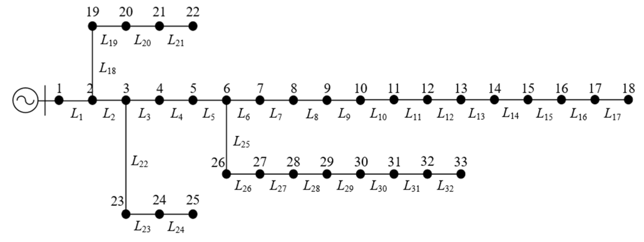
Figure 3.
Fault diagnosis matrix of L28 fault.
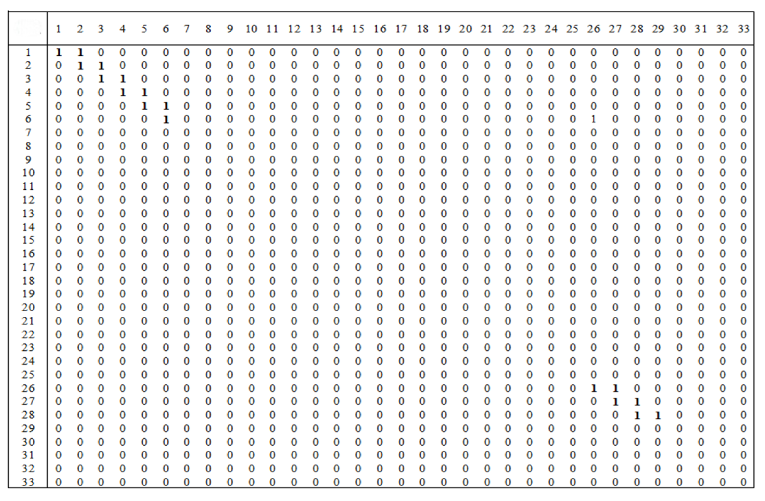
Figure 4.
Fault diagnosis matrix of L8 fault with node 3.
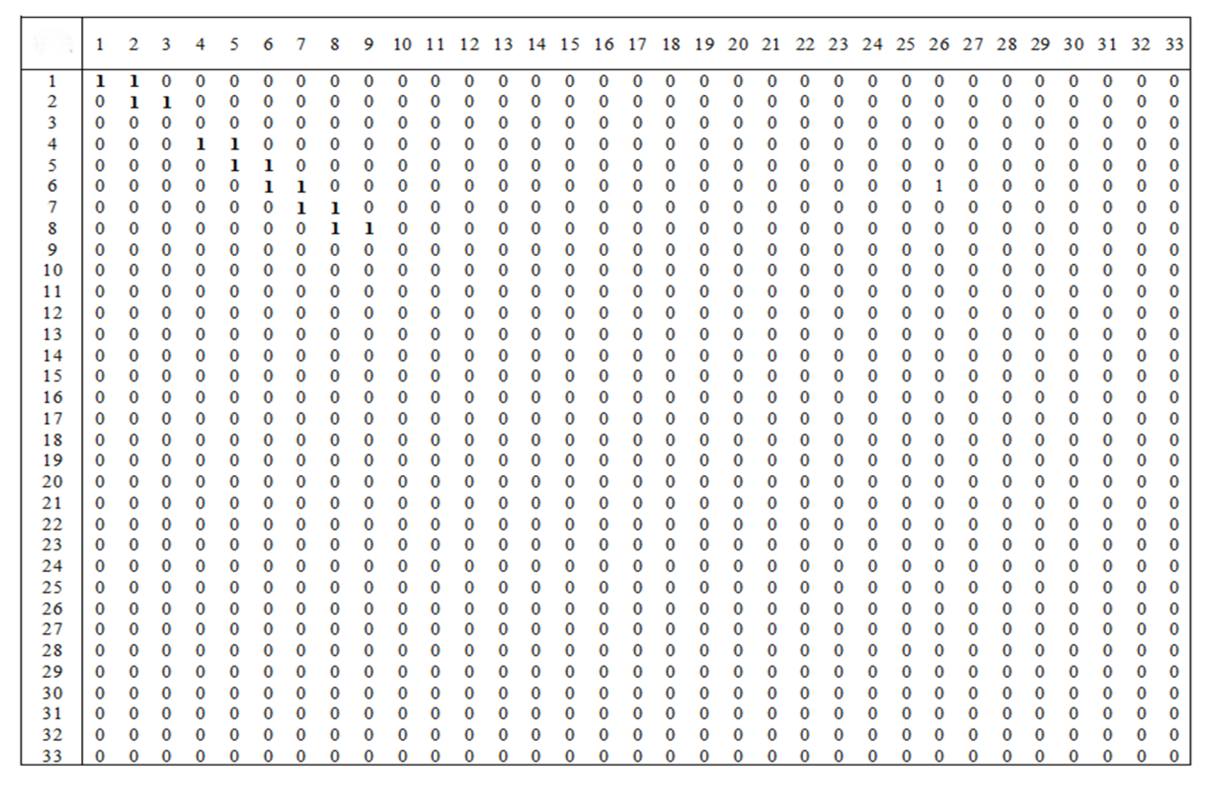
Figure 5.
Fitness curve of L8 fault with node 3 distortion.
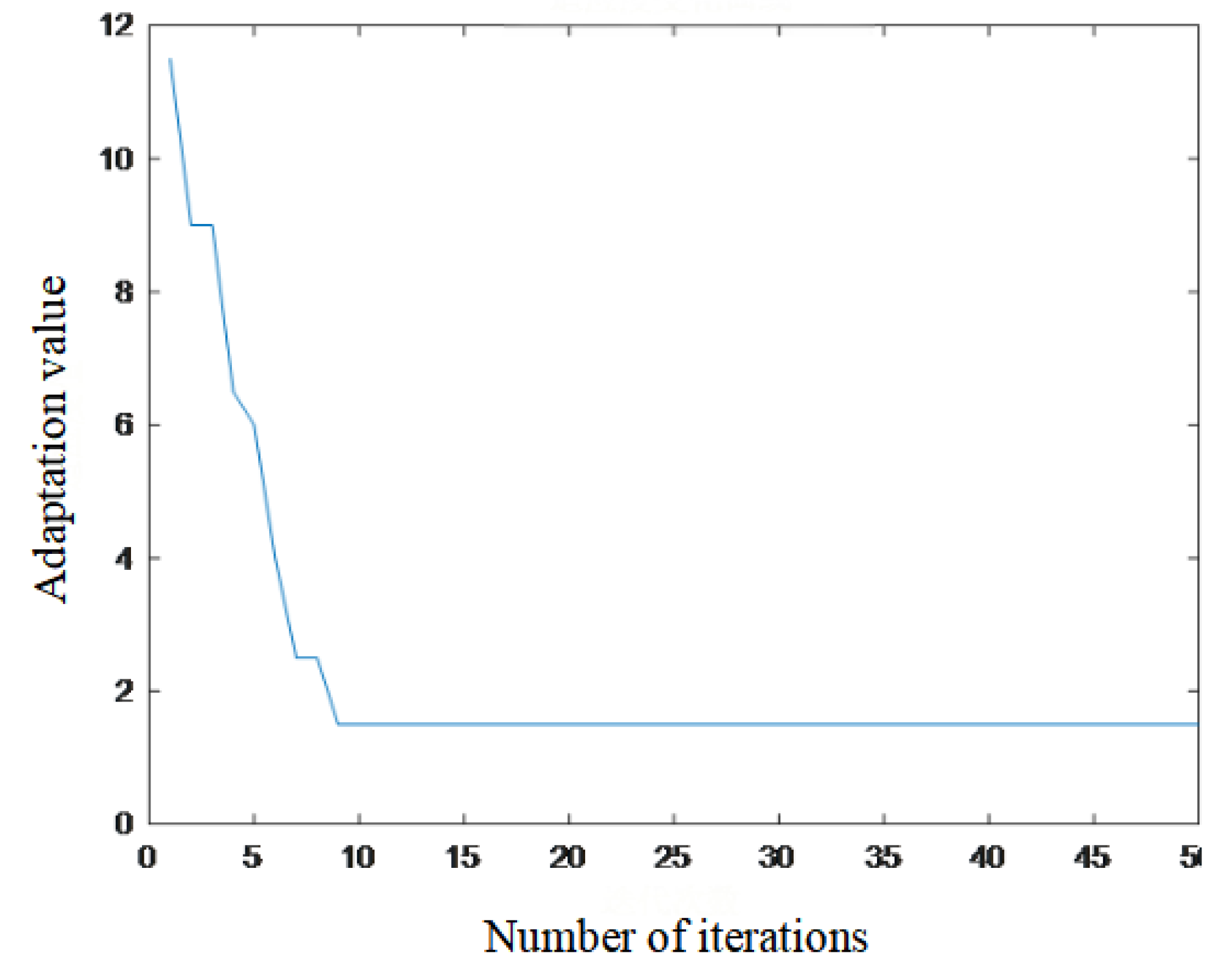
Figure 6.
Fitness curve of L31 fault with node 3, node 4 and node 27 distortions.
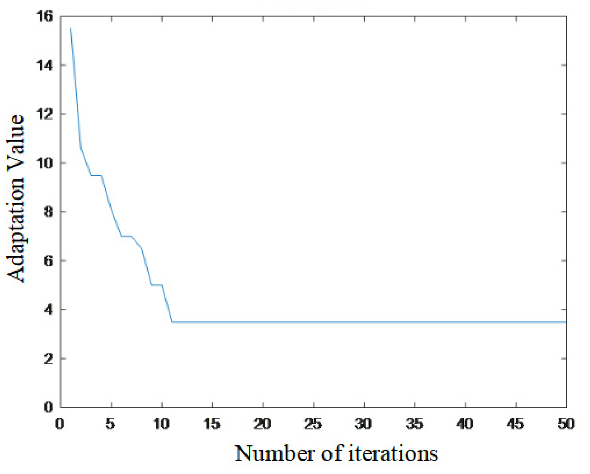
Figure 7.
Comparison of the number of optimization iterations of the IBPSO algorithm and the fusion algorithm.
Figure 7.
Comparison of the number of optimization iterations of the IBPSO algorithm and the fusion algorithm.
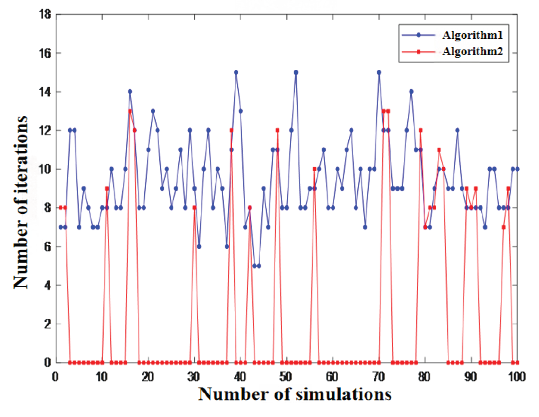

Table 1.
Fault section location results in multiple scenarios.
| Fault Location | Fault condition | Result | ||
| L3 | 0.01 | 0 | [1 1 1 0 0 0 0 0 0 0 0 0 0 0 0 0 0 0 0 0 0 0 0 0 0 0 0 0 0 0 0 0 0] | L3 |
| L7 | 20 | 30 | [1 1 1 1 1 1 1 0 0 0 0 0 0 0 0 0 0 0 0 0 0 0 0 0 0 0 0 0 0 0 0 0 0] | L7 |
| L17 | 30 | 45 | [1 1 1 1 1 1 1 1 1 1 1 1 1 1 1 1 1 0 0 0 0 0 0 0 0 0 0 0 0 0 0 0 0] | L17 |
| L20 | 100 | 90 | [1 1 0 0 0 0 0 0 0 0 0 0 0 0 0 0 0 0 1 1 0 0 0 0 0 0 0 0 0 0 0 0 0] | L20 |
| L26 | 1000 | 30 | [1 1 1 1 1 1 0 0 0 0 0 0 0 0 0 0 0 0 0 0 0 0 0 0 0 1 0 0 0 0 0 0 0] | L26 |
Table 2.
Fault section location results under various node distortions.
| Fault Location | Distortion Node | Node Classification Matrix Result | IBPSO Result | Result | |
| L6 | 13 | [1 1 1 1 1 1 0 0 0 0 0 0 1 0 0 0 0 0 0 0 0 0 0 0 0 0 0 0 0 0 0 0 0] | L6 | - | L6 |
| L11 | 10 | [1 1 1 1 1 1 1 1 1 0 1 0 0 0 0 0 0 0 0 0 0 0 0 0 0 0 0 0 0 0 0 0 0] | L9、L11 | L11 | L11 |
| L21 | 2、26 | [1 0 0 0 0 0 0 0 0 0 0 0 0 0 0 0 0 0 1 1 1 0 0 0 0 1 0 0 0 0 0 0 0] | L1、L21 | L21 | L21 |
| L23 | 16、28 | [1 1 1 0 0 0 0 0 0 0 0 0 0 0 0 1 0 0 0 0 0 0 1 0 0 0 0 1 0 0 0 0 0] | L23 | - | L23 |
| L14 | 4、7、22 | [1 1 1 0 1 1 0 1 1 1 1 1 1 1 0 0 0 0 0 0 0 1 0 0 0 0 0 0 0 0 0 0 0] | L3、L6、L14 | L14 | L14 |
Table 3.
Fault section location results under changes in distribution network topology.
| Fault Location | Fault condition | Result | ||
| L5 | 0.01 | 0 | [1 1 1 1 1 0 0 0 0 0 0 0 0 0 0 0 0 0 0 0 0 0 0 0 0 0 0 0 0 0 0 0 0] | L5 |
| L6 | 20 | 30 | [1 1 1 1 1 1 0 0 0 0 0 0 0 0 0 0 0 0 0 0 0 0 0 0 0 0 0 0 0 0 0 0 0] | L6 |
| L9 | 30 | 45 | [1 1 0 0 0 0 0 0 0 1 1 1 1 1 1 1 1 1 1 1 1 1 0 0 0 0 0 0 0 0 0 0 0] | L9 |
| L20 | 100 | 90 | [1 1 0 0 0 0 0 0 0 0 0 0 0 0 0 0 0 0 1 1 0 0 0 0 0 0 0 0 0 0 0 0 0] | L20 |
| L28 | 1000 | 30 | [1 1 1 1 1 1 0 0 0 0 0 0 0 0 0 0 0 0 0 0 0 0 0 0 0 1 1 1 0 0 0 0 0] | L28 |
Table 4.
Comparison of the positioning performance of the fusion algorithm and basic algorithms.
| Algorithm Type | Number of simulations | Average time required/ms | Average number of iterations | Accuracy rate/% |
| Node Classification Matrix Algorithm | 100 | 1.32 | - | 77 |
| The IBPSO Algorithm | 100 | 202.5 | 9.45 | 94 |
| Fusion Algorithm | 100 | 16.1 | 2.24 | 96 |
Table 5.
Comparison of the positioning accuracy of node classification algorithm and fusion algorithm.
Table 5.
Comparison of the positioning accuracy of node classification algorithm and fusion algorithm.
| Fault Section | Number of Random Node Distortions | Accuracy rate/% | |
| Node Classification Matrix Algorithm | Fusion Algorithm | ||
| L3 | 1 | 83 | 100 |
| 3 | 77 | 97 | |
| L27 | 1 | 82 | 99 |
| 3 | 74 | 96 | |
| L17 | 1 | 80 | 98 |
| 3 | 72 | 95 | |
Disclaimer/Publisher’s Note: The statements, opinions and data contained in all publications are solely those of the individual author(s) and contributor(s) and not of MDPI and/or the editor(s). MDPI and/or the editor(s) disclaim responsibility for any injury to people or property resulting from any ideas, methods, instructions or products referred to in the content. |
© 2025 by the authors. Licensee MDPI, Basel, Switzerland. This article is an open access article distributed under the terms and conditions of the Creative Commons Attribution (CC BY) license (http://creativecommons.org/licenses/by/4.0/).
Copyright: This open access article is published under a Creative Commons CC BY 4.0 license, which permit the free download, distribution, and reuse, provided that the author and preprint are cited in any reuse.


