
Submitted:
29 September 2025
Posted:
30 September 2025
You are already at the latest version
Abstract
Micro-Phasor Measurement Units (µ-PMUs) have emerged as advanced devices for power system monitoring; nevertheless, their high-cost limits large-scale deployment. To address this, optimization algorithms can be employed for their optimal placement (OµPP). This research investigates two optimization techniques for OµPP, aiming to minimize µ-PMU placement costs while maintaining maximum observability. Three cases are analysed: Case 1 (OµPP under normal conditions), Case 2 (OµPP with a single µ-PMU outage), and Case 3 (OµPP considering Zero Injection Buses, ZIBs). Particle Swarm Optimization (PSO) and Grey Wolf Optimization (GWO) are used to solve this problem. MATPOWER version 8.0 is used to obtain the IEEE 33 and 69 distribution bus systems for the case studies. Results show that GWO outperforms PSO in reducing the number of µ-PMUs while ensuring observability, especially in larger systems, while PSO is more effective in smaller systems. Voltage estimation from µ-PMU data is conducted using the WLS algorithm, with three noise levels (0.01, 0.02, 0.04) considered to assess the impact of measurement noise. The findings indicate that increasing µ-PMU placement, as in Case 2, improves voltage estimation accuracy and stability, while a reduced number of µ-PMUs, as in Case 3, shows large deviations and instability under higher noise levels. This analysis highlights the trade-off between cost and reliability in achieving effective monitoring.
Keywords:
distribution systems
; Grey Wolf Optimizer
; maximum observability
; optimal µ-PMU placement
; Particle Swarm Optimization
; voltage estimation
1. Introduction
The Distribution Networks (DNs) have become more prone to transients due to the increasing inclusion of renewable generation, distributed energy sources (DERs), electric vehicles (EVs), and demand-side management (DSM) technologies [1,2]. Although these developments promote sustainability and efficiency, they are also increasing the complexity, variability, and uncertainty of electrical distribution networks. Traditional monitoring and control techniques, which have largely been designed for transmission networks, are generally inadequate for the distribution level, where uneven loads, radial topologies, and prosumers pose significant challenges due to bidirectional energy flows. Supervisory control and data acquisition (SCADA) systems are employed for monitoring and controlling the power networks. However, the latency in SCADA systems, the increased complexity of DNs, and unsynchronized data measurements from SCADA systems hinder the correct state estimation of DNs [3,4,5]. An essential requirement for addressing these issues, situational awareness has become a crucial requirement for the reliable operation of distribution systems. The real-time measurement and monitoring of power systems provide an accurate understanding of the state of the power system for its smooth operation [6,7]. One of the most effective technologies that enables high-level monitoring and situational awareness in modern networks is the micro-phase measurement unit (µ-PMU). It derives from the commonly used phasor measurement units (PMUs) that are utilized in transmission systems; µ-PMUs provide high-precision measurements of voltage and current phasors at the distribution level, with precise timing made possible by GPS synchronization in microseconds. Compared to traditional SCADA systems, µ-PMUs offer superior temporal resolution and accuracy, enabling advanced functions such as fault detection, topology identification, state estimation, and the integration of DERs. Despite these benefits, the installation and maintenance costs of µ-PMUs are a barrier to their implementation, making it impossible to equip every bus in the distribution system with the devices. As a result, the optimal placement of µ-PMUs (OµPP) has emerged as an important research field. The objective of OµPP is to determine the minimum number of µ-PMUs and their best locations that ensure observability, reliability, and resilience, while minimizing costs. Finding the best location is a complex mixed optimization problem, especially in large distribution systems where the network configuration is radial and a greater number of measurements is required for robustness against noise, data errors, or device failures [8,9,10,11,12,13]. Over the years, various optimization techniques have been used, which are mainly divided into mathematical programming methods and heuristic/metaheuristic algorithms. In the preliminary studies, the determination of the optimal location of the PMU is primarily carried out using mathematical programming formulations, such as integer linear programming (ILP), mixed-integer linear programming (MILP), and nonlinear programming (NLP). These methods are appealing because they can provide mathematically correct solutions under well-defined constraints. For example, ILP considers the observation as a set covering problem, where binary decision variables indicate whether a PMU is installed at a bus or not. MILP expands this setup to account for additional aspects such as redundancy and cost functions. Although these methods are theoretically rigorous, they have significant limitations in their practical application. First, the solution space grows combinatorially with the size of the system, making ILP and MILP computationally infeasible for large-scale systems such as IEEE 69 or 118 bus networks [14,15,16]. Second, and more importantly, these methods often rely on theoretical assumptions of perfect measurements. For example, mathematically, a minimal solution may not provide enough additional features, which can result in a loss of observability if a µ-PMU fails. Due to these challenges, researchers have adopted heuristic and metaheuristic algorithms. Unlike exact mathematical programming, meta-optimization algorithms aim to find practically optimal solutions in a reasonable time, even in large, nonlinear, and non-convex search spaces. Their main advantage is that they are flexible, as they can easily integrate practical constraints, such as redundancy requirements and equipment costs, while maintaining scalability for large systems. Furthermore, they are less likely to generate misleading results, as they rely on population-based or adaptive search mechanisms that better capture the irregular nature of systems [17,18].
The importance of optimal placement goes beyond just observation capability. The correct voltage estimation is one of the most important outcomes of implementing µ-PMU. State estimation is the foundation of system monitoring, allowing operators to know the complete bus voltages that describe the operational state of the system. Conventional distribution state estimation methods heavily rely on measurements obtained from SCADA data and load forecasts, both of which face low accuracy and limited resolution. In contrast, µ-PMU provides real-time, high-resolution phase data, significantly enhancing the reliability of estimation. However, due to cost limitations, µ-PMUs cannot be deployed everywhere, and their effectiveness mainly depends on the placement strategy [19,20,21]. When placed optimally, they ensure that critical buses are directly measured, while others can be evaluated using the network's equations and constraints. Placement strategies that consider redundancy further enhance resilience, allowing for error detection and accuracy in the presence of noise or incorrect measurements. The weighted least squares (WLS)[22] method is generally used to estimate voltage, and studies have consistently shown that, in the case of better installation locations, WLS estimates are close to the results of reference power flow, where typically the errors are less than 0.1 p.u. This demonstrates that the accuracy of voltage estimates not only depends on the estimation algorithm but is also closely related to where and how the µ-PMUs are installed. This study builds on these insights by investigating OµPP in 33- and 69-bus distribution systems using PSO and GWO under three scenarios: normal operating conditions, a µ-PMU failure, and the inclusion of ZIBs. In addition to analyzing observation and excessive penetration, the study evaluates the performance of the algorithm in terms of convergence behavior, computation time, and scalability. It validates the effectiveness of the locations through voltage estimates under different noise levels. The main contributions of this article are as follows;
- Two state-of-the-art optimization techniques are utilized to determine the OPP while considering practical constraints. A single µ-PMU outage and ZIBs are considered practical constraints for a comprehensive study.
- ZIBs aid in reducing the required number of µ-PMUs while ensuring observability; hence, strategically placing µ-PMUs by leveraging ZIBs reduces µ-PMUs. Therefore, this condition is explored in this study to decrease the number of µ-PMUs and hence the overall placement cost. When a single µ-PMU fails to operate at a specific bus, it may cause a loss of critical data. Therefore, a case study examining a single µ-PMU failure and its potential impact on cost is also considered.
- After the placement, the WLS algorithm is employed for voltage estimation to ensure that strategically installed µ-PMUs measure the voltage estimation correctly for all case studies.
- Different noise levels are introduced via a change in standard deviations (STDs) to simulate more realistic conditions for the presence of noise in the system to evaluate the impact of noise levels on the state estimation.
The rest of the article is arranged in this manner: Section 2 provides a comprehensive mathematical problem formulation and mathematical modeling of optimization algorithms. Section 3 briefly discusses the methodology. Section 4 provides the results of simulations, while Section 5 provides a detailed discussion about the behavior of both algorithms in terms of convergence and computation time, Section 6 discusses voltage estimation through WLS and its comparison with true voltages obtained from power flow analysis, Section 7 provides an overview of impact of different noise levels on voltage estimation, Section 8 provides an overall discussion while Section 9 concludes the article.
2. Literature Review
Researchers have used various techniques to arrive at the OPP, which range from analytical and mathematical programming methods to heuristic and metaheuristic methods [23]. In ref. [9] Integer linear programming (ILP) is employed for optimal PMU placement (OPP), considering some practical constraints like ZIBs for transmission networks. The authors established that the number of PMUs increases as the topology of the power network changes. In ref. [24] Genetic Algorithm (GA) is employed to achieve the full observability of the IEEE 57 bus system. A smaller number of PMUs is reported while ensuring maximum observability. The authors in ref. [25], employed a greedy search algorithm to obtain a smaller number of PMUs while ensuring maximum observability. In ref. [26], a network compression method is proposed, and a tabu search algorithm is used to reduce the number of PMUs while ensuring the maximum observability. Multiple Optimization techniques can also be hybridized to harness the computational strengths of these approaches, enabling more effective solutions to multiobjective optimization problems. In ref. [27] a hybrid PSO-GSA algorithm is proposed to solve the OPP problem while ensuring full observability. Different practical constraints are considered, and the proposed technique is employed on different case studies. In ref. [28] OPP problem is formulated considering PMU channel cost and risk of operation (RoOP) and solved using ILP. ZIBs are also considered in the formulation, and full observability is ensured. In ref. [29] a new graph theory-based OPP algorithm is proposed to resolve scalability issues while ensuring full observability, taking into account practical constraints like ZIBs. Recently, some studies have focused on PMU installation strategies that are clearly more accurate for voltage estimation in active distribution networks. Salehi et al. proposed a framework based on accuracy in the UK 77-bus test system in ref. [30], in which a multi-objective genetic algorithm (MOGA) was used. Their method reduces the error between actual and estimated voltage profiles, taking cost constraints into account. The results showed that, although a reduced number of PMUs, if placed strategically, can reduce estimation errors to less than 0.5 p.u. Additionally, the study highlighted the importance of additional PMUs, as they mitigate the detrimental effects of erroneous or corrupt input data. Some other contributions have emphasized uncertainty quantification and robustness. Romero et al. in ref. [31] employed a Bayesian optimal experimental design (OED) framework in reference, which directly incorporated the uncertainty of the grid parameter into the placement problem. Their results in the IEEE 14 and 118 bus systems showed that the best design significantly reduced the estimated discrepancy compared to random locations. Building on this, Peng et al. in ref. [32] developed a mixed-integer semidefinite programming (MISDP) model for µ-PMU placement, which was solved through an improved boundary division technique. Their results in IEEE systems showed the overall improvement and scalability of this approach, surpassing both the accuracy and computation duration of conservative and convex techniques. Mishra and de Callafon in ref. [33] extended the problem to networks with partially known admittance parameters, proposing a method that guarantees observability and minimizes noise-induced variance. Their method, which was tested on the 14-bus IEEE network, showed a 10% better performance compared to unconventional designs. Peng et al. in ref. [34] employed the greedy algorithm–based method incorporating information entropy and Monte Carlo–based fault simulations to evaluate PMU placements. Simulated studies revealed significant improvements, with the estimated state error reduced from 1.6% to 0.2% and the loss of observation remaining above 90%. This demonstrates that focusing solely on observation, without considering loss dynamics or redundancy, leads to ineffective solutions. With these works, mixed-integer semidefinite programming methods were also proposed to rigorously include completely loose conditions, which improved the accuracy of state estimates, but require large computational needs. In ref. [35] Tangi and Gaonkar developed a PMU-based voltage estimation framework for active distribution networks. By using numerical linear programming for optimal location, their approach ensured full observability with the minimum number of PMUs in the IEEE 33, 69, and 119 bus test systems. The placement strategy was validated based on the results of forward and backward power flows, showing a nearly perfect match. However, zero injection buses were ignored in the analysis, ensuring that all nodes are included in the estimation process. Their work emphasized that the optimal placement of PMUs not only reduces costs but also enhances the practical performance of active distribution networks under the integration of renewable energies.
3. Methodology
3.1. Mathematical Formulation of µPMU Placement
In this section, a mathematical model for the OµPP problem is presented, with an emphasis on maximizing the observability with the fewest possible µ-PMUs to reduce the cost. The formulation includes three case studies: Normal Condition, Consideration of ZIBs, and Single µ-PMU outage.
3.1.1. Objective Function
The primary objective of the OµPP is to minimize the number of µ-PMUs to reduce the cost while ensuring the observability of all buses. The objective function is given as;
Subject to In equation 1, N represents the total number of buses in the power system, is the binary decision variable, which can be 1 or 0, showing whether a µ-PMU is placed at the specific bus, and c is the cost of each µ-PMU. A represents a connectivity matrix showing the connection of buses.
The connectivity matrix is a square symmetric matrix that can also be written as
X is a matrix and represents the binary decision variable for installing µ-PMU, and b is the observability matrix, which is the minimum bus observability necessary for each bus.
3.1.2. Case Studies
In this article, different case studies are presented to thoroughly test the proposed approach, ensuring the power system stays fully observable under different conditions, such as normal operation, a single µ-PMU failure, and the presence of Zero Injection Buses (ZIBs).
Observability Under Normal Conditions
Under normal conditions, each bus must be either directly or indirectly observable by at least a single µ-PMU.
where, represents the set of buses connected to the bus (entailing bus itself). This condition ensures that each bus is either directly or indirectly observable.
Observability Considering Zero Injection Buses
Zero injection buses are buses with no connected load or generator; zero current injection, active power (Pd) and reactive power (Qd) measurements are also zero at these buses. ZIBs can be manipulated to reduce the required number of µ-PMUs while ensuring observability. As the sum of currents is zero and the line impedances are negligible, the voltage and current at the adjacent buses to ZIB can be calculated using Kirchhoff's current and voltage laws. A way of appending the ZIBs in OPP formulation is as follows.
In equation 7, represent the ZIBs, and is the set of adjacent buses to the bus , including itself.
Observability During Single µ-PMU Outage
To ensure that the network remains observable even if a PMU fails, the effectuation condition is that each bus must be observed by two µ-PMUs either directly or indirectly. The single µ-PMU outage condition can be formulated as;
In equation 8, for each bus if there is no PMU placed on the bus, it must be observable by a µ-PMU on the neighboring buses. This ensures that even if a µ-PMU at the bus fails, the bus remains observable through a second µ-PMU.
3.2. System Observability Redundancy Index
SORI is an analysis used to determine the robustness and redundancy of the PMU placement configuration. SORI determines how well a system is observed using PMUs. Mathematically, SORI can be determined as;
N is the total number of buses in the system under consideration. To get the mean value, we can divide SORI by the total number of buses in the system.
3.3. Optimization Algorithms
To solve the OµPP problem, this article employs two state-of-the-art optimization algorithms, PSO and GWO, leveraging their unique strengths in global exploration and local exploitation to achieve an efficient and robust solution.
3.3.1. Particle Swarm Optimization
PSO is a population-based optimization algorithm inspired by the social behavior of bird flocks. It is widely used in solving problems related to optimization. A set of particles is first initialized by placing random particles in the search space. The particles change their place with a specific set velocity, and the position of the particle determines the placement of the µ-PMU. Both the velocity and position of particles are initiated randomly within the bounds of the µ-PMU placement problem, i.e. either µ-PMU is to be placed or not. The particles progress toward the best solution at each iteration based on the experience of their previous position. In the algorithm, pbest is the personal best experience of a particle, and gbest is the global best solution. The velocity of each particle is updated based on the previous position of the particle, the cognitive component (how close it is to its personal best solution), and the social component (how close it is to the global best solution). The equation for velocity is given as;
is the inertia weight that controls the impact of the previous velocity, and are cognitive and social coefficients, respectively, and and are the random values between 0 and 1. The position is updated as per equation 12.
The position is then clamped to the binary domain via equation 13;
By using 0.5 as a threshold value, binary quantization is performed to convert the continuous values into binary numbers. It divides the binary values into two equal parts, such that values greater than 0.5 to 1 and less than 0.5 to 0. This thresholding ensures that optimization works in a continuous search space; however, the placement decision remains binary as per the OPP problem requirement 0.5 is chosen as it is the midpoint between 1 and 0.
3.3.2. Grey Wolf Optimization
GWO is also an optimization technique that is inspired by the hunting behavior of grey wolves. It simulates the social hierarchy within a wolf pack, where alpha, beta, and delta wolves guide the entire pack during the hunt. For the OPP problem, GWO aims to find the optimal µ-PMU placement by utilizing the social hierarchy and collective intelligence of the grey wolf pack. Each wolf represents a solution for µ-PMU placement, where the position of the wolf is the binary vector of values (0 or 1). The number of wolves is predefined, and the position of each wolf is initialized randomly within the search space. The wolves update their positions based on the position of alpha, beta, and delta wolves (the best, second-best, and third-best) solutions. The equation for the position is given as;
In equation 15, A =2 × a × rand () – a, where a decreases linearly from 2 to 0. , , and represent the distance between the current position of wolves and their distance from alpha, beta, and delta wolves, respectively.
where , , and are the coefficients that control the movement of wolves.
3.4. Fitness Function
The fitness function evaluates how well a µ-PMU placement satisfies the observability constraints with the minimum number of µ-PMUs.
is the placement of µ-PMU on the bus (1 if placed or otherwise 0), and is the penalty factor for unobserved buses.
Here, shows the number of µ-PMUs that are directly or indirectly observing the bus , if it is zero, a penalty is imposed in the fitness function.
3.5. Filtration
A filtration process is employed for all three case studies to remove the redundant µ-PMUs after evaluating their placement. The primary purpose of filtration is to ensure that each bus in the system is observable with the minimum possible µ-PMUs. It ensures that the final µ-PMU placement avoids over-coverage to reduce the cost while maintaining observability. In normal conditions, the filtration consists of two passes, in the first pass, the process marks all the buses as observed, either a µ-PMU is placed on the bus, or it is connected to the bus on which a µ-PMU is already placed. In the second pass, the filtration process rigorously checks if any µ-PMU is redundant, and if a bus is covered by multiple µ-PMUs and no unique observation is achieved from an extra µ-PMU, it is removed. In case of a single µ-PMU outage at a certain bus, some critical data might be lost; therefore, it is necessary to have other PMUs observing that bus. In the first pass of the filtration process, all buses are marked as observed if they are either directly monitored by a µ-PMU or indirectly observable through neighbouring buses. This ensures that even if a µ-PMU fails at a specific bus, the system can maintain observability through alternative observation paths. The second pass explores any redundant PMUs, removes them, and adds additional µ-PMUs for loss of coverage if necessary. In the case of ZIBs, the same method is followed as in normal conditions; however, the filtration process focuses on placing the µ-PMU adjacent to ZIBs, because the voltage, current, and phase angles at ZIBs can be calculated using Kirchhoff’s laws.
3.6. State Estimation Using MATPOWER and WLS Algorithm
State estimation is a crucial parameter for estimating the power flows, voltage magnitudes, and angles for the smooth operation of power systems. In this article, for the true estimation of voltage magnitudes and angles, MATPOWER power flow is employed. The estimation of voltages and currents is performed using the WLS method, and the real values of the angles and magnitudes for the parameters are extracted from the estimated results obtained after implementing the WLS algorithm. The update principle adjusts the state vector to align it with the noisy measurements. The process is repeated until the residuals are minimal, providing accurate estimates of real system conditions.
The power flow equations used to calculate the true values of voltage magnitudes and angles are given as;
In (18) and (19), and are active and reactive powers, and are the voltage magnitudes of buses and , and are the voltage angles at buses and , and are the conductance and susceptance between buses and , respectively.
The WLS method [22] is a very effective approach to estimate the state of unsupervised buses. It uses existing measurements and assigns weights based on their accuracy, improving the accuracy and stability of the electrical system state estimation. The objective is to identify the magnitude of the voltage, the phase angle, and the power flow of those buses that are being monitored, using the available measurements, which include the power flow and the voltage magnitude of the monitored buses. A nonlinear measurement function can be used to represent the PMU measurement model, as shown in equation (20).
The measurement function h(x), which is based on the current state vector x, generates expected measurement values. The noise in the measurement is represented as e, while z is the measurement vector. By mapping the state vector x in the measurement space, this function determines the magnitude of the expected voltage, the voltage angle, and the magnitude of the current for a specific state. The predicted values for the magnitude of the voltage, the voltage angle, and the magnitude of the current are provided through equations (21) and (22).
The current magnitude , and current angle on the branch between bus and bus j can be calculated from (23), (24), and (25).
In equation (23), the branch entry between buses and is represented as . The voltage values at buses i and j are represented in equation (23) as and , respectively. The phase angle of the current flowing through the branch is represented in equation (24) as . Equation (26) defines the residual vector , which represents the difference between the vector of observed measurements and the values of estimated measurements . This vector captures the errors or discrepancies between the actual measurement and the expected measurement.
In equation (26), the measured vector with noise, which represents the actual measurements obtained from the PMUs and is affected by noise, is denoted as z. The measurement function, corresponding to the expected measurements according to the current state vector, is presented as h(x). The Jacobian matrix H, as shown in equation (27), includes partial derivatives that demonstrate how changes in the state variables (such as voltages and angles) affect the measurements. These partial derivatives show the sensitivity of the measurements to changes in the state variables and provide an estimate of the estimated values. The nonlinear measurement function is linearized around the current state estimate using this matrix.
The weight matrix W in equation (28) represents the level of confidence in the data. It is a diagonal matrix where each measurement is assigned the inverse value of the variance. Measurements with higher noise receive a lower weight, while measurements with higher confidence (and lower noise) receive a higher weight. In the basic case, the standard deviation (std) is set to 0.01 p.u.
In the literature, the values of the different standard deviations (STDs) are evaluated to determine their effect on the state estimates [36]. To ensure that the most reliable measurements have a more significant impact on the final state estimates, the weight matrix W assigns more weight to measurements with lower uncertainty. Measurements with lower standard deviations receive more weight, indicating less noise, while measurements with higher standard deviations receive less weight, indicating more noise. This approach improves the accuracy of state estimates by reducing the effect of noise or uncertain measurements. By minimizing dependence on erroneous information and emphasizing the more precise measurements, this method ensures a more reliable estimation process. In the WLS stage, the state vector x is updated iteratively to minimize the total sum of the weighted squared residuals.
Δx is calculated using (30).
In Eq. (30), H is the Jacobian matrix, calculated in Eq. (27). W is the weight matrix, calculated in Eq. (28), and r represents the measurement error, or the remaining vector, derived in Eq. (26). The algorithm proceeds repeatedly as long as the update step , as shown in Eq. (31), is quite small, indicating that the estimates have become constant. The limit is set at a small price to ensure harmony, usually 10−6. The update vector criterion serves as the basis for the consistency criteria, determining when the algorithm is sufficiently integrated into an accurate state approximation.
This error has been added by applying these standard deviations (voltage value, voltage angle, current value, and current angle) described in the algorithm as () to reflect real-world conditions. In this part of the algorithm that uses ZIBs, adopting the WLS method for voltage estimation ensures that the effect of zero injection is captured accurately. As a result, highly precise and reliable state estimates are obtained, effectively modelling the behavior of this system while also considering the effects of these specific buses.
3.7. Procedures For Placement Of µ-PMUs
- The placement of µ-PMUs in a radial distribution system consists of multiple steps elucidated in detail in this section.
- In the first step, data regarding IEEE bus systems is uploaded from MATPOWER version 8.0 onto the MATLAB program. IEEE 33 and 69 distribution systems are represented in Figure 1.
- In the second step, a connectivity matrix is formed based on the connections between buses in both distribution systems.
- After the formation of the connectivity matrix, initial parameters for both algorithms are initialized, and the fitness function is defined. The main objective of the fitness function is to reduce the number of PMUs while ensuring full observability for all cases. Three case studies are performed for both the 33 and 69 bus systems, i.e., under normal conditions, with Zero Injection buses, and a single PMU outage. ZIBs are identified to leverage them to reduce the PMUs for network observability.
- Simulations are performed, and as the fitness criteria are achieved, the program stops and generates a binary vector consisting of 0’s and 1’s indicating on which buses PMUs are installed. The flowcharts for both PSO and GWO are shown in Figure 2.
- WLS algorithm is employed on selected buses via both algorithms for voltage estimation, and different noise levels are introduced for validating the placement of PMUs.
4. Simulations & Results
This section describes the optimal placement of µ-PMUs under different conditions. The simulations are performed in MATLAB 2018 on a Dell 12th Gen Intel (R) Core (TM) i5-1235U @ 1.30 GHz and 16 GB RAM. The simulations are conducted on both IEEE 33 and 69 distribution bus systems.
4.1. Case 1: OµPP Under Normal Conditions
Under normal operating conditions, the IEEE 33-bus system requires a maximum of 11 µ-PMUs to ensure complete observability. Complete observability is achieved with 11 µ-PMUs from both PSO and GWO algorithms. The value of SORI is 34, with a mean value of 1.0303, indicating that every bus is being observed by at least one µ-PMU on average. This demonstrates the efficiency of GWO in achieving observability with fewer PMUs while maintaining a high level of redundancy.
A total of 25 µ-PMUs are placed by the PSO algorithm for the IEEE 69 Bus system for complete observability, while with GWO, 24 µ-PMUs are obtained. The value of SORI for PSO is 76 with a mean value of 1.1014, and GWO had a SORI of 70 with a mean value of 1.014, which is slightly lower than PSO; however, it also indicates that each bus is being observed by at least one µ-PMU. Figure 3 and Figure 4 show the placement of µ-PMUs for both algorithms, indicating that even though GWO has placed a lower number of PMUs, it has still achieved complete observability.
Table 1 provides detailed information on the PMU placements, costs incurred, and other critical metrics for the case study.
4.2. Case 2: OµPP With A Single µPMU Outage
Under the condition of a single µ-PMU outage, the number of required µ-PMUs increases to ensure system reliability. In this scenario, each bus must be observed by at least two µ-PMUs to maintain complete observability. This redundancy ensures that if one µ-PMU fails, the system remains fully observable, as the other µ-PMUs continue to collect data either directly or indirectly from the affected bus. For the 33-bus system, both the PSO and GWO algorithms yielded a total of 25 PMUs under the single µ-PMU outage condition, as shown in Figure 5. The SORIs for PSO and GWO are 72 and 71, respectively, with mean SORI values of 2.1818 and 2.1515.
Similarly, for the 69-bus system, both algorithms resulted in 53 µ-PMUs, with SORI values of 156 for PSO and 155 for GWO, and mean SORI values of 2.261 and 2.246, respectively. Figure 6 illustrates the placement of µ-PMUs, which clearly shows that each bus is observable by a sufficient number of PMUs, ensuring that the bus remains observable even if a PMU fails.
The SORI values indicate that each bus is observed by a minimum of two µ-PMUs, ensuring system reliability and observability even in the event of a µ-PMU failure. This redundancy guarantees uninterrupted monitoring and enhances overall resilience. Table 2 below shows the buses on which PMUs are placed and other critical metrics for case study 2.
4.3. Case 3: OPP Considering ZIBs
ZIBs can be leveraged to reduce the number of µ-PMUs. In the IEEE 33 Bus system of the MATPOWER version, there are no ZIBs; hence, the number of µ-PMUs remains the same as in normal conditions, which is 11. For the IEEE 69 Bus system, 20 buses are identified as ZIBs, and hence, they can be leveraged to reduce the required number of µ-PMUs. In the case of PSO, the optimization results indicate that a total of 18 µ-PMUs are required, achieving an SORI of 79 and a mean value of 1.1449. On the other hand, GWO demonstrates improved efficiency, requiring only 17 µ-PMUs with an SORI of 71 and a mean value of 1.029. Figure 7 shows the OPP for both PSO and GWO algorithms considering ZIBs. This comparison highlights the superior performance of GWO in reducing the number of µ-PMUs while maintaining system observability. Both methods effectively leverage ZIB properties to optimize placement, but GWO achieves a more cost-effective solution with fewer devices and a slightly lower redundancy level. The mean values confirm that all buses remain observable by at least one µ-PMU, ensuring reliable monitoring across the network. Table 3 provides a summary of µ-PMUs placed in case 3.
The comparative analysis revealed that GWO performed better than the other optimization techniques, achieving a lower number of PMUs while ensuring complete observability. The comparison with existing techniques also revealed almost similar results, which are presented in Table 4.
4.4. Comparison of PSO and GWO
In this section, the performance of both PSO and GWO is assessed based on two critical factors, computation time and convergence of all case studies. These two factors are considered essential for evaluating the efficiency and effectiveness of algorithms in solving optimization problems. The total number of particles/wolves is taken to be 100, and each algorithm is run for 1000 iterations.
4.4.1. Computation Time
The efficacy of an algorithm is determined by some key parameters, and computation time is one of the key parameters that determines the efficiency of the algorithm in terms of processing time. The computation time is determined for all the case studies, which is presented in Table 5. The results of the analysis of the computational time show a clear distinction between the performance of PSO and GWO as the size of the electricity system increases. Although PSO works significantly faster on smaller systems (33 buses), the computational time increases dramatically when applied to larger systems (69 buses), to more than 577 seconds for the 69-bus system in Case Study 1, compared to GWO's 212 seconds. This suggests that PSO may be struggling with scalability, with the increased complexity of larger systems requiring more iterations and processing time. On the contrary, GWO shows a more stable and gradual increase in computational time, which means that larger systems are processed more efficiently. While GWO scales better, its performance is not completely free of inefficiencies, as seen in Case Study 2, where it took 5.26 seconds for the 69-bus system, which is slightly higher than the 3.31 seconds of PSO in the same case. PSO is more efficient for smaller systems, but can become computationally expensive as the system size increases, while GWO is found to be more consistent at different scales, albeit at higher computational costs for medium and large systems. Table 5 presents the time taken by each algorithm for different case studies.
The analysis from the Table 5 provides a clear overview of each algorithm and also suggests that the choice between these algorithms should depend on the specific requirements of the application: PSO may be suitable for real-time and smaller-scale optimization tasks, while GWO may be a better choice for systems on a larger scale where accuracy and robustness overcome computational time limitations. The result for case study 3 also reveals that PSO takes comparatively lower time than GWO to converge to a solution for the 69-bus system. This also shows that PSO faces a scalability issue. It works efficiently with smaller systems, but GWO shows a stable convergence for larger systems.
4.4.2. Convergence Behavior
In Case Study 1, which evaluated the 33- and 69-bus systems, the PSO algorithm demonstrated rapid convergence in the smaller system. In the 33-bus system, the number of μ-PMUs placed quickly stabilized in the initial iterations, indicating that PSO is highly efficient in identifying a viable solution for smaller systems, as depicted in Figure 8 (a). However, the algorithm showed minimal sophistication after the initial convergence, as it crashed quickly, suggesting that while PSO is fast, it may not be exploring the search space thoroughly enough to further refine the solution. However, the performance of the 69-bus system showed a different trend, as shown in Figure 9 (a). The PSO showed significant fluctuations in the number of PMUs issued, especially after the initial placements. These fluctuationssuggest that PSO is struggling to maintain an optimal solution as the complexity of the system increases. Despite the initial convergence rate, the tendency of PSOs to be stuck in local optima on larger systems limits overall effectiveness in achieving optimal placement, as it takes much longer for the algorithm to stabilize μ-PMU placement.
In Case Study 2, the 33-bus system again highlighted the efficiency of PSO, as shown in Figure 10(a). The algorithm showed rapid convergence, and the number of PMUs placed quickly stabilized. As in case study 1, the initial rapid convergence of PSO was followed by limited additional refinement, suggesting that it may not be able to fully explore the solution space for optimal placement in smaller systems. For smaller systems, GWO also shows similar behavior and converges quickly. However, GWO started from the minimum number of PMUs and increased the number of μ-PMUs before arriving at an optimal solution. This demonstrates GWO's ability to better explore the search space and avoid premature convergence to a local optimum, as shown in Figure 10 (b). Although PSO was faster, GWO's stable and gradual approach resulted in a more reliable placement over a more extended period, highlighting its robustness for an optimal solution.
For the 69-bus system in Case Study 2, PSO again showed large fluctuations in the number of μ-PMUs placed, indicating that it is struggling to cope with the increasing complexity of the system. The PSO algorithm showed rapid but erratic convergence, with several oscillations in the μ-PMU placement process. This behavior amplifies the challenges of PSO with large-scale systems, where its tendency to get caught up in local optima becomes more pronounced. On the other hand, the GWO showed a more stable convergence in Case Study 2, showing a smooth progression towards the final solution. The algorithm's ability to place μ-PMUs gradually without large jumps or fluctuations suggests that GWO is better suited to the 69-bus system, depicting more reliable results at the expense of longer computational time. For the same case study, the PSO remained faster but less stable, while the GWO showed consistency and robust performance, especially for larger energy systems where solution optimality and stability are critical. The behavior of both algorithms can be observed in Figure 10 and Figure 11.
Figure 12 (a) represents the convergence for both PSO and GWO applied to the 69-bus system in case study 3. The figures show the number of μ-PMUs placed throughout the iterations. The graph shows that the number of μ-PMUs remains fairly stable across all iterations in the case of PSO, with a sharp increase at the beginning of the process, followed by minimal changes. This indicates a rapid synchronization in the early stages and very few subsequent adjustments afterwards. On the other hand, Figure 12 (b) shows the convergence behavior of the GWO algorithm applied to the same 69-bus system. It can be observed that in the beginning, the number of μ-PMUs increases rapidly and becomes steadier over time, reflecting a more stable convergence pattern. This suggests that although PSO converges comparatively faster, the GWO maintains a more consistent but slower optimization process, potentially better suited for more complex systems with lower placement sensitivity.
In summary, the results in Case Study 1, Case Study 2, and Case Study 3 suggest that while PSO offers faster convergence in smaller systems, it becomes less effective in larger, more complex networks due to its tendency to converge prematurely or get stuck in local minima. GWO, on the other hand, shows more stable and gradual convergence, making it better suited to larger systems, albeit at the cost of longer computational times. The choice between PSO and GWO depends on the size and complexity of the system, with PSO being the preferred choice for speed in smaller systems and GWO being the best choice for larger systems that require robustness and optimality.
5. Voltage Estimation with MATPOWER and the WLS method
The evaluation of voltage estimation is provided using the WLS method to compare with the actual value obtained from MATPOWER's power flow to determine the robustness of the PMU location. For a detailed study, three different case studies with varying numbers of PMUs and bus locations have been considered to determine the accuracy of the PMU placement. Finally, for each case study, two levels of STD noise have been introduced for comparative analysis. Figure 13 presents the results of the voltage intensity estimation after the PMU placement using the PSO and GWO algorithms for the IEEE 33 and 69 bus systems. Figure 13 (a) shows the voltage profile of the IEEE 33 bus system after the PMU location optimization using the PSO and GWO algorithms. The estimated voltage intensities remain very close to the reference values from the MATPOWER power flow analysis, demonstrating that the PMU placement is effective in providing accurate voltage estimates throughout the system. Similarly, figures 13 (b) and (c) show the voltage estimation results for the IEEE 69-bus system, where the PMUs have been placed using the PSO and GWO algorithms, respectively. In both cases, the estimated voltage values are close to the reference values, indicating that the PMU placement using both optimization algorithms ensures reliable voltage estimates. The results confirm that the selected PMU locations are strategically placed to provide accurate voltage estimates, which validates the effectiveness of PMU placement optimization in the 33 and 69-bus systems using PSO and GWO. In Figure 14 (a), for the IEEE 33 bus system, the estimated error remains relatively low in most buses, with deviations that generally stay below 0.1 p.u. Similarly, Fig. 14 (b) and (c) show the voltage estimation error for the IEEE 69-bus system. In both cases, the error stays below 0.1 p.u. for most of the buses, with a few buses showing larger errors, particularly around bus 60 in the case of the 69-bus system. However, these deviations remain within an acceptable limit, indicating that the PMU placements using both optimization algoithms are still effective in providing accurate voltage estimates.
Figure 15 describes the results of the voltage estimation for Case Study 2. In Figure 15 (a), the IEEE 33-bus system with PSO placement shows that the estimated voltage values (orange line) align well with the actual values (blue line) obtained from the power flow analysis, with only minor changes observed. Figure 15 (b) shows similar accuracy for the GWO algorithm in the 33-bus system, where the estimates are quite close to the actual values and there are minor differences. In Figure 15 (c), for the IEEE 69 Bus system, a slight fluctuation between the buses can be observed in the voltage estimation when using PSO, but overall, this estimation is reliable. Similarly, in Figure 15 (d), the GWO algorithm provides a more consistent voltage profile, with fewer variations, indicating better accuracy compared to PSO in large systems. Overall, Figure 14 shows that both PSO and GWO perform well in the correct placement of PMUs for voltage estimation, while GWO, especially in the large IEEE 69 bus system, provides more consistent and precise results.
In Figure 16 (a) and (b), for the IEEE 33-bus system, the estimated losses remain low, often staying below 0.015 p.u., with some deviations around bus 25, which are within an acceptable limit for both PSO and GWO. In Figure 16 (c) and (d), for the IEEE 69-bus system, the error often stays below 0.01 p.u., with a few larger errors near bus 30 in the case of PSO. However, these errors remain acceptable, indicating that both algorithms effectively ensure accurate voltage estimation for both systems
In Figure 17, the estimation of voltage magnitude results for Case Study 3 in the IEEE 69-bus system using PSO and GWO algorithms are shown. In (a), with the PSO placement, significant spikes and errors are found in the WLS estimates, particularly around bus 60. These deviations are due to the limited number of PMUs that are installed, which affects the observability of the system and leads to less accurate estimates. Similarly, in (b), using the GWO algorithm, the voltage estimation also indicates significant errors and instability. This is due to the inadequate number of PMUs placed, resulting in insufficient observability and higher estimation errors. Both cases demonstrate a lack of complete observability.
Figure 18 presents the estimated error in voltage magnitudes obtained using PSO and GWO algorithms with PMUs in the IEEE 69 bus system for Case Study 3. In (a), the PSO algorithm exhibits significant errors in voltage estimates, particularly around bus 60, where the error exceeds 0.25 p.u. The distribution of errors exhibits considerable variance across several buses, primarily due to the limited number of PMUs, which hinders the ability to observe the entire system. Similarly, in (b), with the installation of GWO, the error remains significant, especially at bus 60, where errors also reach approximately 0.25 p.u. Estimated errors in voltage magnitudes at other buses also show considerable fluctuations. These higher errors are primarily due to the smaller number of PMUs and the lack of observation of the entire system, leading to unreliable voltage magnitude estimates.
5.1. Impact Of Variation In Noise Levels On Voltage Estimation
For further investigation of the robustness of placement, varying noise levels were introduced, and the results were compared for each case study. Two levels of noise are introduced, which are 0.02 and 0.04, to observe the effects on estimation, and deviations in estimated values from reference values are observed. In Figure 19, the results of the voltage estimation from MATPOWER power flow and the WLS estimation are presented in case study 1 under different levels of noise for both the IEEE 33 and 69 bus systems. With a low noise level of 0.02 STD, figures 19 (a)-19(c) show that the voltage estimation results remain close to the true values, with only slight deviations in most buses. When the noise level is increased to 0.04 STD, as shown in figures 19 (d)–19(f), the differences between the expected and reference voltages become more evident. Several buses, especially in the IEEE 69-bus system, show significant estimation errors and fluctuations. These large discrepancies underscore the sensitivity of PMU data to high noise levels, which can be exacerbated by faulty or malicious data. Such distortions affect the reliability of state estimates and, as a result, can lead to incorrect conclusions about the operational conditions of the system.
In Figure 20, the voltage magnitude for case study 2 is estimated under different noise levels, for both IEEE 33-bus and 69-bus systems. At a low noise level of 0.02 STD, as shown in Figure 20 (a), 20 (b), 20 (c), and 20 (d), the voltage estimations are closer to the true voltage value. The deviations are minimal, indicating the reliability of data obtained from the strategic placement of PMUs when the measurement noise is relatively small. The estimation errors further exacerbate as depicted in figures 20 (c), 20 (d), 20 (g), and 20 (h); when the noise level rises above 0.04 STD, nevertheless, they are still less severe than in case study 1. Even so, the deviations remain relatively small, especially in the IEEE 69-bus system, where the voltage profiles continue to closely follow the reference values. This highlights how greater measurement redundancy and improved observability can significantly reduce the influence of higher noise levels. A significant reason for the lesser deviations in case study 2 is the strategic placement of more PMUs, as each bus is monitored by at least two PMUs. This additional precaution ensures that measurements are more trustworthy and less impacted by noise or faulty data. Even when some measurements are inaccurate, having several independent observations increases the robustness of the voltage estimation, minimizing big variations and boosting overall state estimation accuracy.
Figure 21 shows the results of Case Study 3 for the IEEE 69-bus system. At a lower noise level of 0.02 STD (Figs. 21 (a) and 21 (b)), placement using either algorithm produces voltage magnitude estimates that largely match true voltage values, while substantial variations arise at numerous buses due to reduced observability. When the noise level rises to 0.04 STD (Figs. 21 (c) and 21 (d)), these discrepancies worsen, resulting in considerable mismatches and instability in the estimated profiles. This demonstrates that Case Study 3 results in reduced observability and measurement redundancy, making the estimation more sensitive to noise and less reliable overall, regardless of whether PSO or GWO is used for placement.
6. Discussion
The results of three case studies have demonstrated that the location of PMUs plays a decisive role in ensuring observability and the accuracy of estimates. In case study 1, complete observability was achieved with a minimum number of μ-PMUs, and both PSO and GWO were effective, with GWO requiring slightly fewer devices in a 69-bus system. This shows that the cost of infrastructure can be reduced through strategic location while still maintaining redundancy. However, when the level of noise increases, significant estimation errors occur in case study 1 due to limited redundancy, especially in large systems. The convergence analysis reveals significant differences between various algorithms. It is observed that the PSO has a fast convergence behavior, especially in small systems, making it suitable for real-time applications. However, in large networks, the PSO has shown instability and sensitivity to local minima. In contrast, the GWO converges more gradually, but with greater stability across all system sizes. This demonstrates that while the PSO is effective for small systems, the GWO is more suitable for large and more complex networks where robustness is needed. Voltage estimation behavior under noisy conditions emphasizes the necessity of redundancy. In Case Study 2, with at least two μ-PMUs per bus, estimation errors remained low even at greater noise levels. These redundancy requirements reinforce the measurement's noise tolerance and the possibility of erroneous data, demonstrating that redundancy requirements are just as crucial as algorithm selection for reliable monitoring. However, Case Study 3 demonstrates the perils of aggressively reducing the PMU count. Although optimization reduced the number of placements, it weakened observability, resulting in substantial variations and unreliable voltage estimates when noise levels increased. These findings show that, while algorithmic efficiency and cost reductions are vital, they should not come at the expense of redundancy and reliability. Overall, the findings underline the importance of balancing computing efficiency, convergence stability, and measurement redundancy in order to achieve accurate and resilient power system monitoring.
7. Conclusion
This work optimized μ-PMU placement using Particle Swarm Optimization (PSO) and Grey Wolf Optimization (GWO) for the IEEE 33- and 69-bus systems, with a focus on observability, convergence, and voltage estimation accuracy. In Case Study 1, both algorithms achieved complete observability in the IEEE 33-bus system with 11 μ-PMUs, while for the IEEE 69-bus system, PSO resulted in 25 μ-PMUs and GWO 24, demonstrating greater efficiency. In Case Study 2, redundancy requirements increased the placements to 25 μ-PMUs for the IEEE 33-bus system and 53 for the IEEE 69-bus system, ensuring observability even under single μ-PMU failure. In Case Study 3, leveraging Zero Injection Buses (ZIBs) in the IEEE 69-bus system reduced the requirement to 19 μ-PMUs for PSO and 18 for GWO. Convergence and voltage estimation analyses provided further insights into algorithm performance. PSO converged faster and performed well in the IEEE 33-bus system, but showed instability and erratic behavior in the 69-bus system. GWO, while slower, converged more smoothly and consistently, proving more effective in larger, complex networks. Voltage estimation results revealed that Case Study 2 achieved the most reliable outcomes, as redundancy minimized deviations even under higher noise levels. By contrast, Case Study 1 suffered greater deviations due to limited redundancy, while Case Study 3, though efficient in terms of fewer μ-PMUs, exhibited larger errors under noise. Overall, PSO is more suitable for smaller systems requiring speed, whereas GWO provides stable and robust solutions for larger systems. Voltage magnitude estimation under different noise levels further highlighted the impact of PMU placement strategies. In Case Study 1, limited redundancy led to larger deviations under high noise levels, particularly in the IEEE-69 system. Case Study 2, with redundant μ-PMU placement, demonstrated much lower estimation errors, confirming that redundancy enhances resilience against noise and insufficient data. Case Study 3, while efficient in terms of fewer μ-PMUs, exhibited reduced observability and higher estimation errors, especially at higher noise levels, emphasizing the trade-off between cost-effectiveness and reliability. Overall, this study demonstrates that optimal μ-PMU placement must balance three dimensions: minimizing device count, ensuring robust observability, and maintaining reliable voltage estimation under uncertainty. PSO is more efficient for smaller systems due to its faster convergence, while GWO proves more effective for larger, complex systems owing to its stability and global search capability. The key contributions of the presented work are the utilization of μ-PMU placement to determine the voltage estimation from placement locations. After the placement of μ-PMUs in all three case studies, voltage is estimated with the WLS algorithm with three different noise levels to determine the impact of noise levels. It is observed that the values from the WLS method were close to reference values from the power flow results. However, as the values of noise are increased, the discrepancies in the estimated values also augment, especially in Case Study 1 and Case Study 3. OµPP is crucial for larger distribution systems, which consist of distributed energy sources and require real-time monitoring. The power grids are evolving into more dynamic and decentralized power systems, necessitating the importance of OµPP. Large power systems are highly intricate; therefore, multiobjective optimization can be employed to satisfy the multiple conflicting objectives for OµPP. Future work will explore multi-objective and hybrid optimization approaches to better balance device count, computational efficiency, and estimation reliability in evolving smart grids. Hybrid optimization methods, combining classical algorithms with AI-based techniques, can also be leveraged to reduce computational burden in larger power systems, which the authors aim to explore in future studies.
Author Contributions
Conceptualization, Asjad Ali, Noor Izzri Abdul Wahab, Mohammad Lutfi Othman, and Rizwan A. Farade; methodology, Asjad Ali, Noor Izzri Abdul Wahab; software, Asjad Ali; validation, Mohammad Lutfi Othman, and Rizwan A. Farade; formal analysis, Husam S. Samkari, and Mohammed F. Allehyani, Mohammad Lutfi Othman; investigation, Asjad Ali, and Noor Izzri Abdul Wahab; resources, Asjad Ali, Noor Izzri Abdul Wahab, and Mohammad Lutfi Othman, Rizwan A. Farade; data curation, Husam S. Samkari, and Mohammed F. Allehyani; writing—original draft preparation, Asjad Ali; writing—review and editing, Noor Izzri Abdul Wahab; visualization, Husam S. Samkari, and Mohammed F. Allehyani; supervision, Noor Izzri Abdul Wahab, Mohammad Lutfi Othman, and Rizwan A. Farade; project administration, Asjad Ali, Noor Izzri Abdul Wahab, and Rizwan A. Farad; funding acquisition, Husam S. Samkari, and Mohammed F. Allehyani. All authors have read and agreed to the published version of the manuscript.
Funding
This research was funded by the Ministry of Higher Education (MOHE) of Malaysia under the Fundamental Research Grant Scheme (FRGS/1/2023/TK07/UPM/02/8).
Institutional Review Board Statement
Not applicable.
Informed Consent Statement
Not applicable.
Data Availability Statement
Data will be provided upon reasonable request.
Acknowledgments
The authors would like to thank the associated institutions for providing a conducive environment for conducting this study.
Conflicts of Interest
The authors declare that they have no conflicts of interest.
References
- Asyikin, N.; Radzi, M.; Member, S.; Zainal, A.M. Active Electric Distribution Network : Applications, Challenges, and Opportunities. IEEE Access 2023, 11, 134655–134689. [Google Scholar]
- Dixit, A.; Chowdhury, A.; Saini, P. A review on optimal placement of phasor measurement unit ( PMU). In System Assurances; Elsevier Inc., 2022; pp. 513–530 ISBN 9780323902403.
- Agudo, M.P.; Franco, J.F.; Tenesaca-Caldas, M.; Zambrano-Asanza, S.; Leite, J.B. Optimal placement of uPMUs to improve the reliability of distribution systems through genetic algorithm and variable neighborhood search. Electr. Power Syst. Res. 2024, 236, 110910. [Google Scholar] [CrossRef]
- Bhattacharjee, R.; De, A. A Novel Bus-Ranking-Algorithm-Based Heuristic Optimization Scheme for PMU Placement. IEEE Trans. Ind. Informatics 2023, 19, 9921–9932. [Google Scholar] [CrossRef]
- Khanam, N.; Rihan, M.; Hameed, S. PMU-data assisted state estimation of distribution network with integrated renewables : a comprehensive review. Bull. Electr. Eng. Informatics 2025, 14, 2456–2470. [Google Scholar] [CrossRef]
- Khanjani, N.; Moghaddas-Tafreshi, S.M. An ILP model for stochastic placement of μPMUs with limited voltage and current channels in a reconfigurable distribution network. Int. J. Electr. Power Energy Syst. 2023, 148, 108951. [Google Scholar] [CrossRef]
- Maji, T.K.; Acharjee, P. Multiple Solutions of Optimal PMU Placement Using Exponential Binary PSO Algorithm for Smart Grid Applications. IEEE Trans. Ind. Appl. 2017, 53, 2550–2559. [Google Scholar] [CrossRef]
- Negi, S.S.; Kishor, N.; Singh, A.K. PMUs data based detection of oscillatory events and identification of their associated variable: Estimation of information measures approach. Sustain. Energy, Grids Networks 2024, 39, 101457. [Google Scholar] [CrossRef]
- Su, H.; Wang, C.; Li, P.; Liu, Z.; Yu, L.; Wu, J. Optimal placement of phasor measurement unit in distribution networks considering the changes in topology. Appl. Energy 2019, 250, 313–322. [Google Scholar] [CrossRef]
- Wang, X.; Xia, T.; Li, Y.; Mao, W. Two-stage optimal PMU placement for distribution systems. Meas. Control (United Kingdom) 2024. [CrossRef]
- Kim, B.H.; Kim, H. PMU Optimal Placement Algorithm Using Topological Observability Analysis. J. Electr. Eng. Technol. 2021, 16, 2909–2916. [Google Scholar] [CrossRef]
- Saleh, A.A.; Adail, A.S.; Wadoud, A.A. Optimal phasor measurement units placement for full observability of power system using improved particle swarm optimisation. IET Gener. Transm. Distrib. 2017, 11, 1794–1800. [Google Scholar] [CrossRef]
- Tapas Kumar Maji, P.A. Multiple Solutions of Optimal PMU Placement Using Exponential Binary PSO Algorithm for Smart Grid Applications Tapas Kumar Maji Parimal Acharjee. IEEE Trans. Ind. Appl. 2017, 53, 2550–2559. [Google Scholar] [CrossRef]
- Fotopoulou, M.; Petridis, S.; Karachalios, I.; Rakopoulos, D. A Review on Distribution System State Estimation Algorithms. Appl. Sci. 2022, 12, 1–21. [Google Scholar] [CrossRef]
- Chung, S. Artificial Intelligence Applications in Electric Distribution Systems : Post-Pandemic Progress and Prospect. Appl. Sci. 2023, 13, 1–16. [Google Scholar] [CrossRef]
- Johnson, T.; Moger, T. A critical review of methods for optimal placement of phasor measurement units. Int. Trans. Electr. ENERGY Syst. 2021, 31, 1–25. [Google Scholar] [CrossRef]
- Bairwa, S.K.; Singh, S.P. PMU Placement Optimization Techniques for Complete Power System Observability. J. Chengdu Univ. Technol. 2021, 26, 1–11. [Google Scholar]
- Netto, M.; Krishnan, V.; Zhang, Y.; Mili, L. Measurement placement in electric power transmission and distribution grids : Review of concepts, methods, and research needs. IET Gener. Transm. Distrib. 2022, 805–838. [Google Scholar] [CrossRef]
- Biswal, C.; Sahu, B.K.; Mishra, M. Real-Time Grid Monitoring and Protection : A Comprehensive Survey on the Advantages of Phasor Measurement Units. Energies 2023, 16, 1–34. [Google Scholar] [CrossRef]
- Swain, A.; Abdellatif, E.; Mousa, A.; Pong, P.W.T. Sensor Technologies for Transmission and Distribution Systems : A Review of the Latest Developments. Energies 2022, 15, 1–37. [Google Scholar] [CrossRef]
- Vijaychandra, J.; Ram, B.; Prasad, V.; Darapureddi, V.K. A Review of Distribution System State Estimation Methods and Their Applications in Power Systems. Electron. 2023, 12, 1–16. [Google Scholar] [CrossRef]
- Meriem, M.; Omar, S.; Bouchra, C.; Abdelaziz, B.; Faissal, E.M.; Nazha, C. Study of State Estimation Using Weighted Least Squares Method. Int. J. Adv. Eng. Res. Sci. 2016, 3, 55–63. [Google Scholar]
- Paramo, G.; Bretas, A.; Meyn, S. Research Trends and Applications of PMUs. Energies 2022, 15, 1–32. [Google Scholar] [CrossRef]
- Venugopal, P.; Devaraj, D.; Isaac, J. Optimal Placement of PMU with Complete Observability using Genetic Algorithm. 2024 IEEE Int. Conf. Intell. Tech. Control. Optim. Signal Process. INCOS 2024 - Proc. 2024; 1–4. [Google Scholar] [CrossRef]
- Jaiswal, V.; Thakur, S.S.; Mishra, B. Optimal placement of PMUs using Greedy Algorithm and state estimation. In Proceedings of the 1st IEEE International Conference on Power Electronics, Intelligent Control and Energy Systems, ICPEICES 2016; 2017; pp. 3–7. [Google Scholar]
- Xu, Q.; Yu, L.; Wang, Y.; Kong, X.; Yuan, X. Optimal PMU Placement for the Distribution System Based on Genetic-Tabu Search Algorithm. 2019 IEEE PES Innov. Smart Grid Technol. Asia, ISGT 2019, 2019; 980–984. [Google Scholar] [CrossRef]
- Laouid, A.A.; Mounir Rezaoui, M.; Kouzou, A.; Mohammedi, R.D. Optimal PMUs Placement Using Hybrid PSO-GSA Algorithm. Proc. - 2019 4th Int. Conf. Power Electron. their Appl. ICPEA 2019 2019, 1, 1–5. [Google Scholar] [CrossRef]
- Mukherjee, M.; Roy, B.K.S. Cost-Effective Operation Risk-Driven µPMU Placement in Active Distribution Network Considering Channel Cost and Node Reliability. Arab. J. Sci. Eng. 2023, 48, 6541–6575. [Google Scholar] [CrossRef]
- Mukherjee, M.; Roy, B.K.S. Optimal μPMU Placement in Radial Distribution Networks Using Novel Zero Injection Bus Modelling. SN Comput. Sci. 2023, 4. [Google Scholar] [CrossRef]
- Salehi, A.; Fotuhi-firuzabad, M.; Fattaheian-dehkordi, S.; Lehtonen, M. A PMU Placement Framework in an Active Distribution Network Based on Voltage Profile Estimation Accuracy. 2023 IEEE PES GTD Int. Conf. Expo. 2023, 92–97. [Google Scholar] [CrossRef]
- Romero, I.; Marcia, R.; Petra, N. Optimal PMU Placement for State Estimation with Grid Parameter Uncertainty. In Proceedings of the IEEE PES Grid Edge Technologies Conference & Exposition (Grid Edge); IEEE, 2025. 1–5.
- Peng, Y.; Wu, Z.; Gu, W.; Member, S. Optimal Micro-PMU Placement for Improving State Estimation Accuracy via Mixed-integer Semidefinite Programming. J. Mod. POWER Syst. CLEAN ENERGY 2023, 11, 468–478. [Google Scholar] [CrossRef]
- Mishra, A.; Callafon, R.A. De Optimal PMU Placement for Voltage Estimation in Partially Known Power Networks. 2023 62nd IEEE Conf. Decis. Control 2023, 455–460. [Google Scholar] [CrossRef]
- Peng, Y.; Wu, Z.; Fang, C.; Zheng, S.; Zhao, J. Optimal PMU Placement in Distribution Networks for Improving State Estimation Accuracy and Fault Observability. IEEE Sustain. Power Energy Conf. 2021, 1413–1418. [Google Scholar] [CrossRef]
- Gaonkar, D.N. Voltage Estimation of Active Distribution Network Using PMU Technology. IEEE Access 2021. [Google Scholar]
- Chen, Y.; Ma, J. A mixed-integer linear programming approach for robust state estimation. J. Mod. Power Syst. Clean Energy 2014, 2, 366–373. [Google Scholar] [CrossRef]
- Khanam, N.; Rihan, M.; Hameed, S. Placement of Micro-PMUs and Voltage Estimation in Radial Distribution Networks with Zero Injection constraints. Conf. Proc. - 13th IEEE Power Energy Soc. Innov. Smart Grid Technol. - Asia, ISGT Asia 2024 2024. [CrossRef]
Figure 1.
IEEE Distribution Bus Systems.

Figure 2.
Algorithm Implementation (A) PSO Algorithm (B) GWO Algorithm.
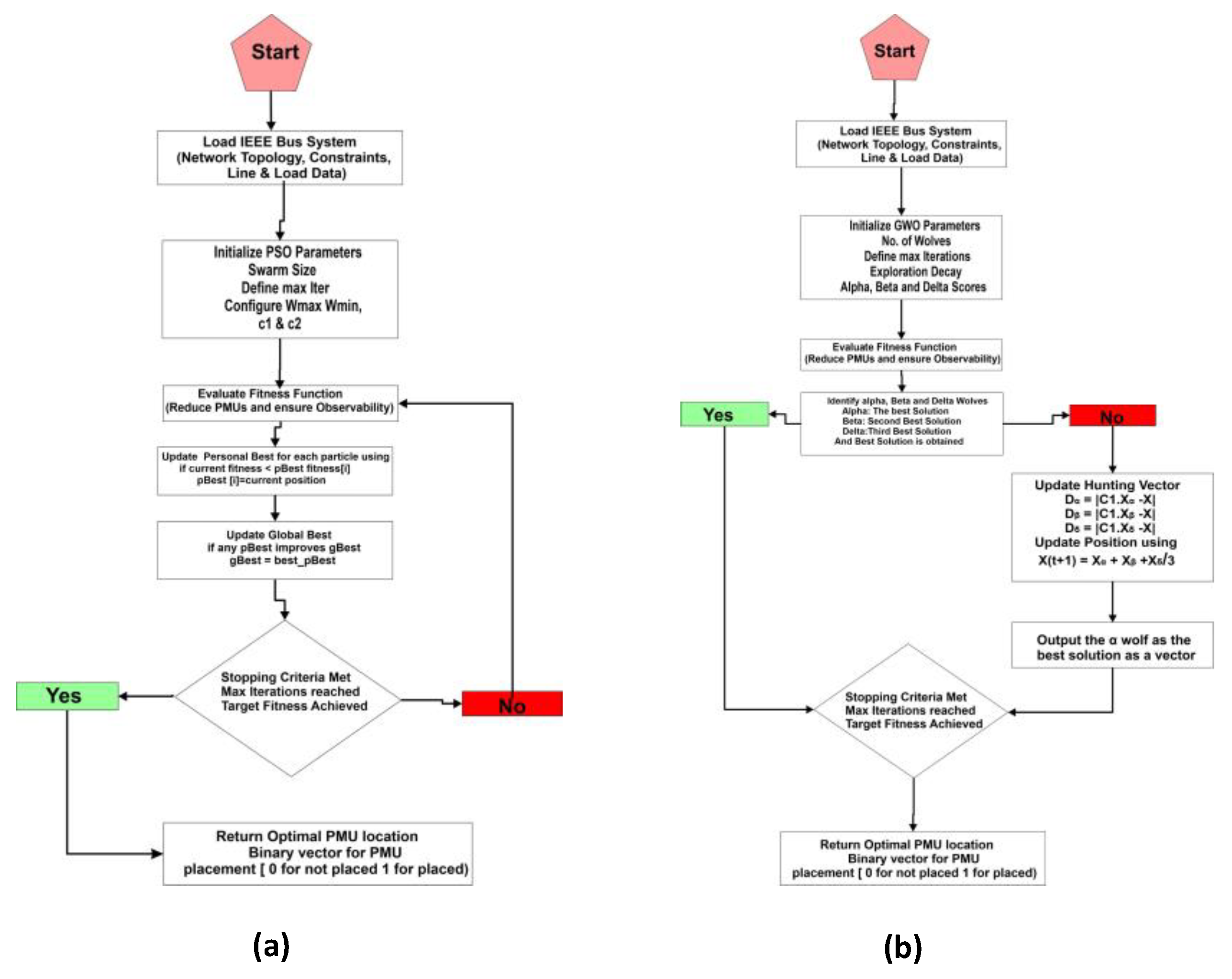
Figure 3.
IEEE 33 Bus System With µ-PMUs Placement for Case 1.
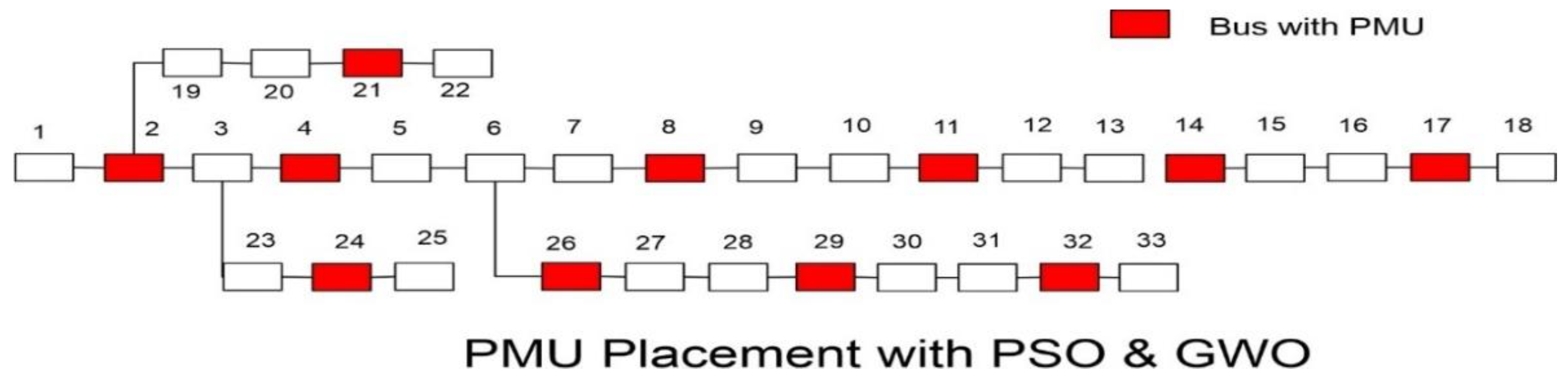
Figure 4.
IEEE 69 Bus System With µ-PMUs Placement for Case 1.
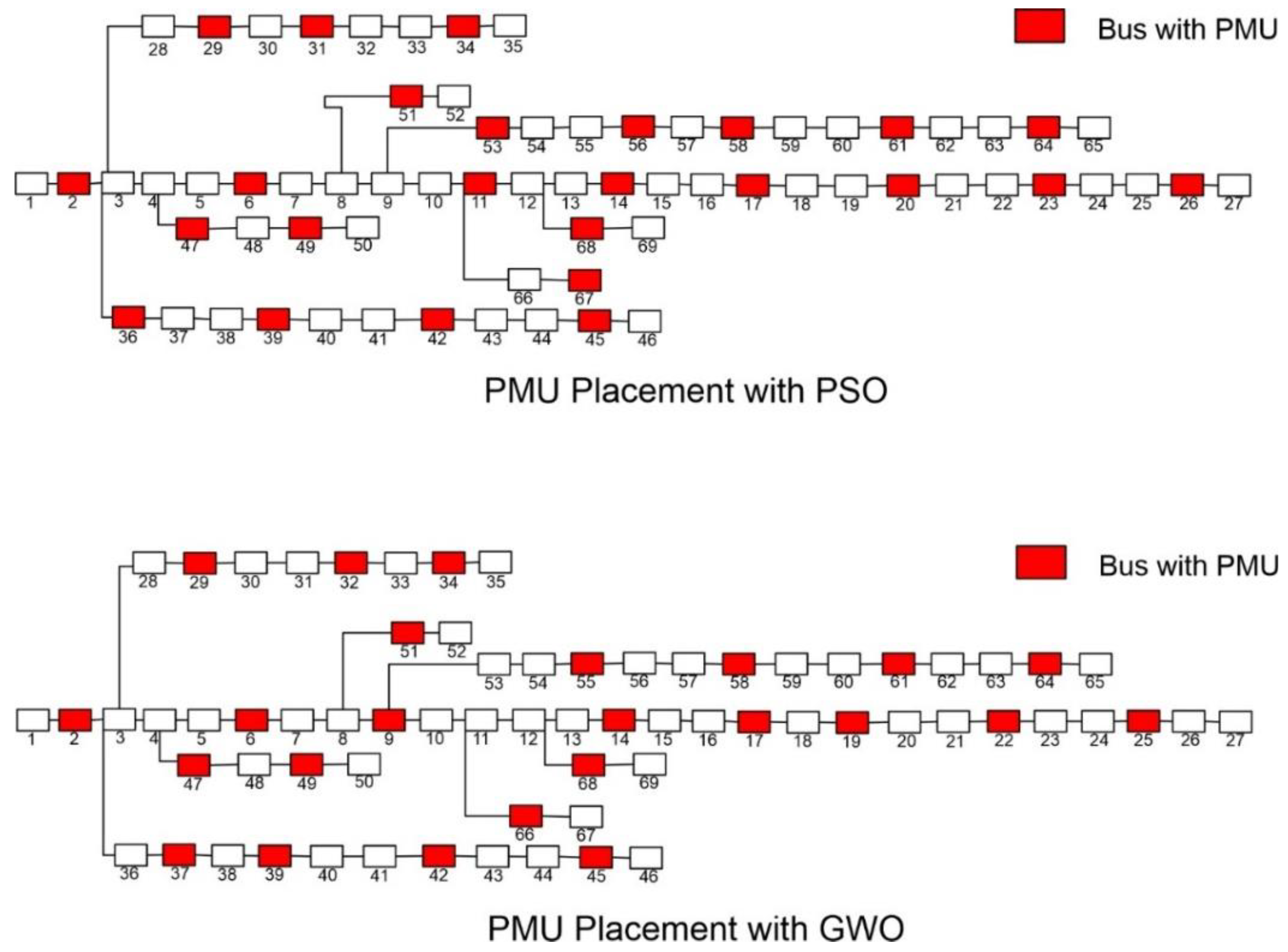
Figure 5.
IEEE 33 Bus System With µ-PMUs Placement for Case 2.
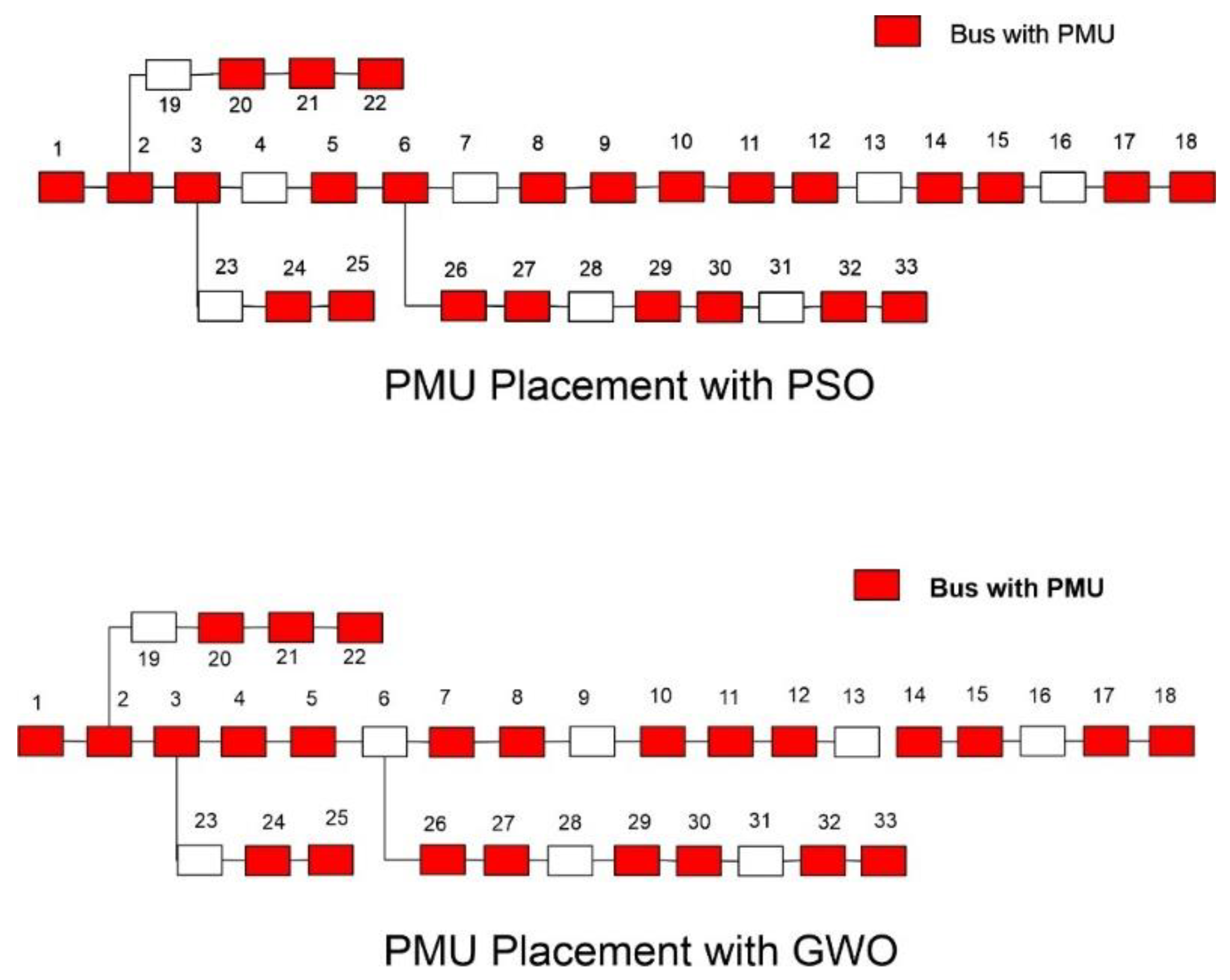
Figure 6.
IEEE 69 Bus System With µ-PMUs Placement for Case 2.
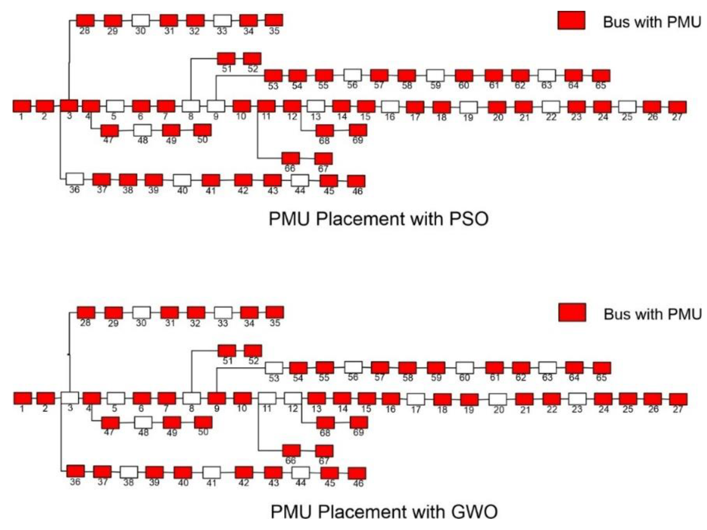
Figure 7.
IEEE 69 Bus System with ZIBs & µ-PMUs Placement for Case 2.
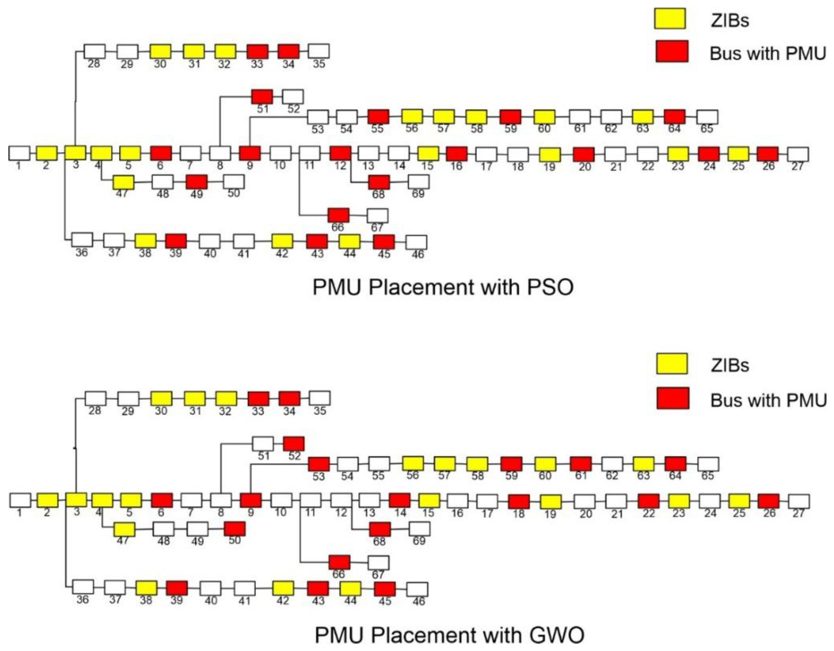
Figure 8.
Case 1 Convergence Graph (a) PSO (b) GWO for 33 Bus System.
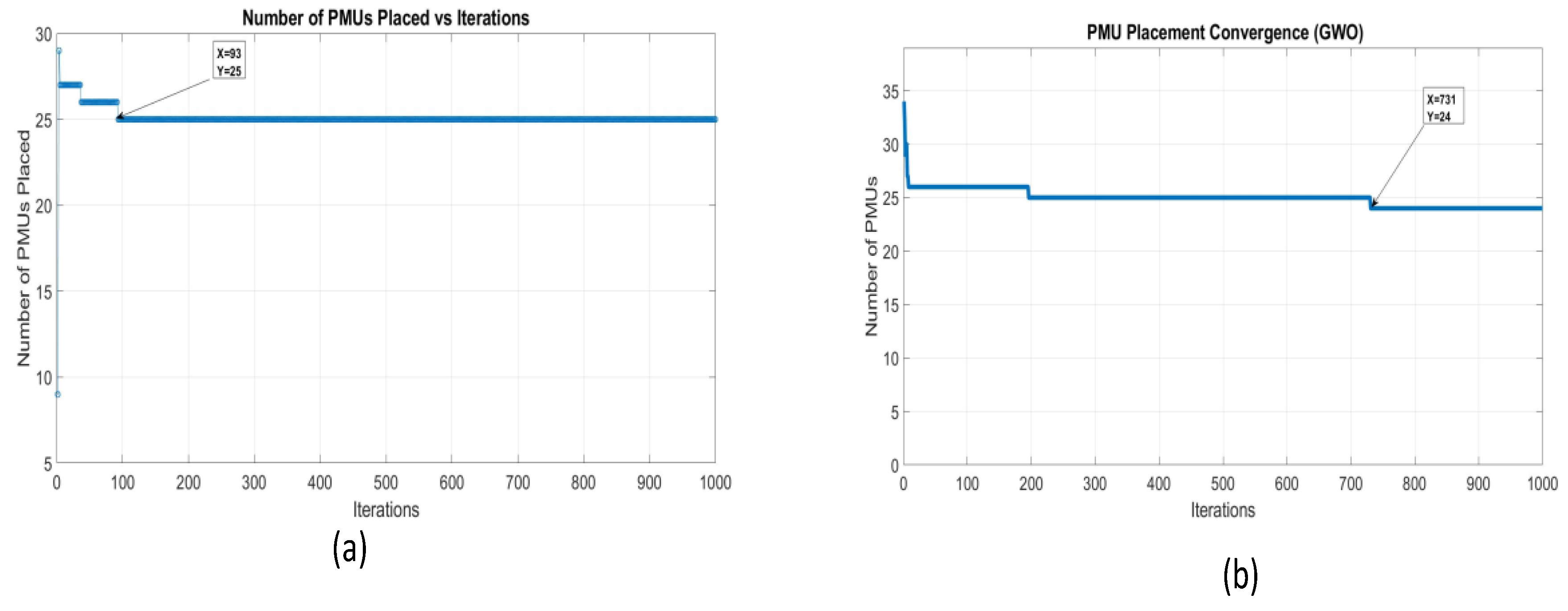
Figure 9.
Case 1 Convergence Graph (a) PSO (b) GWO for 69 Bus System.
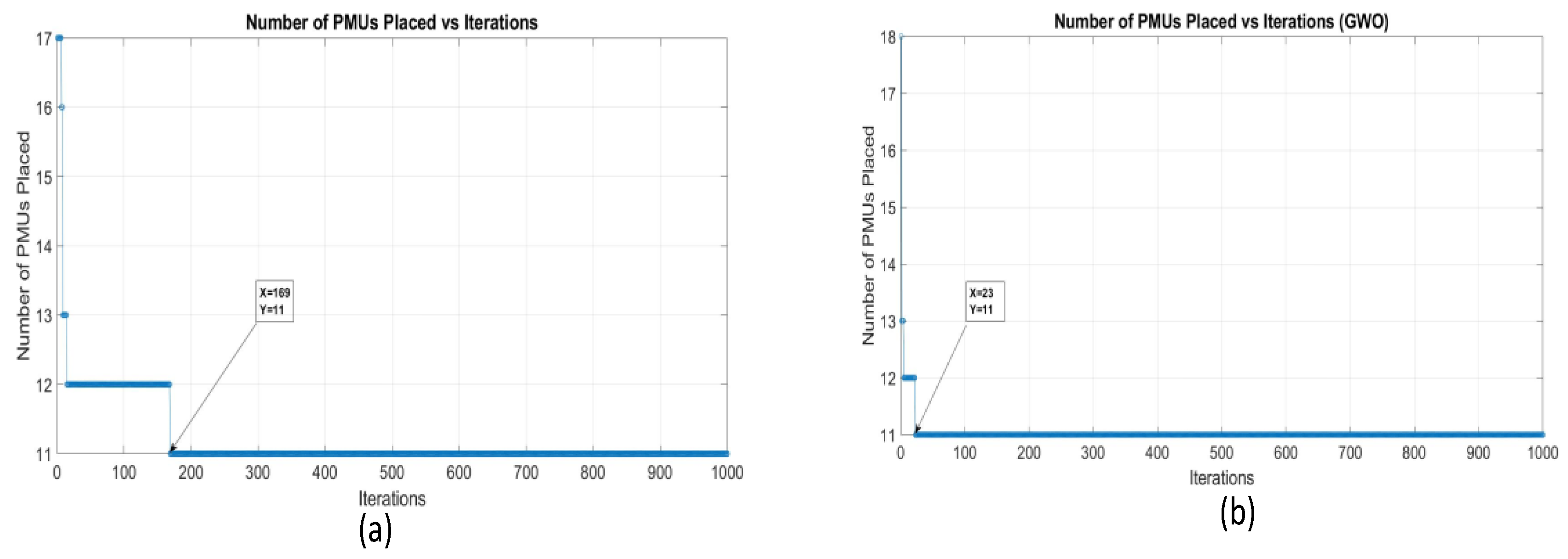
Figure 10.
Case 2 Convergence Graph (a) PSO (b) GWO for 33 Bus System.
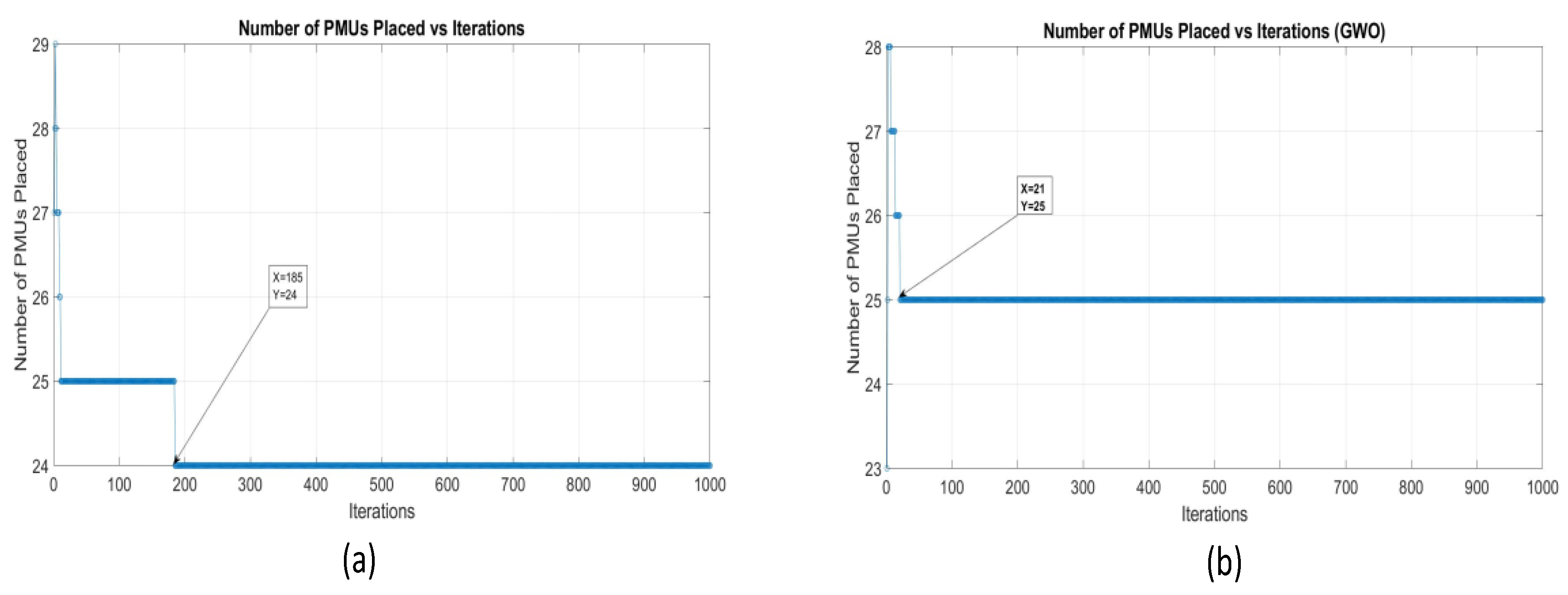
Figure 11.
Case 2 Convergence Graph (a) PSO (b) GWO for 69 Bus System.
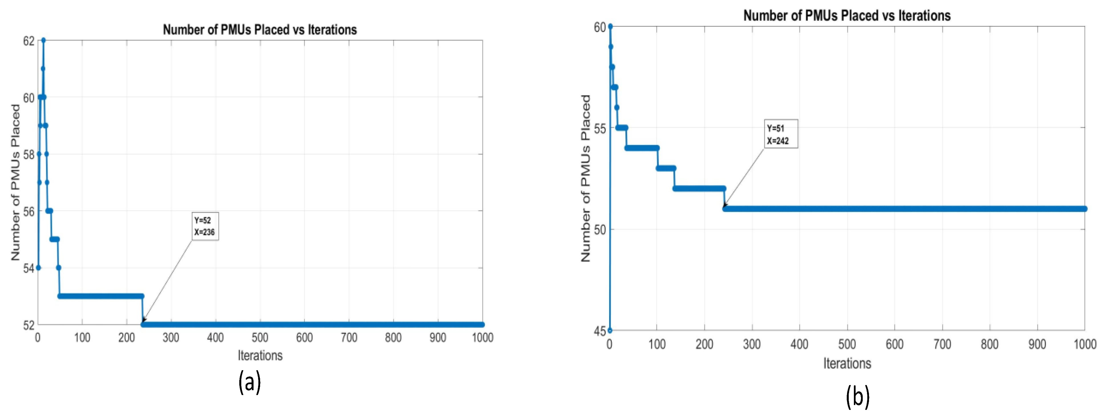
Figure 12.
Case 3 Convergence Graph (a) PSO (b) GWO for 69 Bus System.
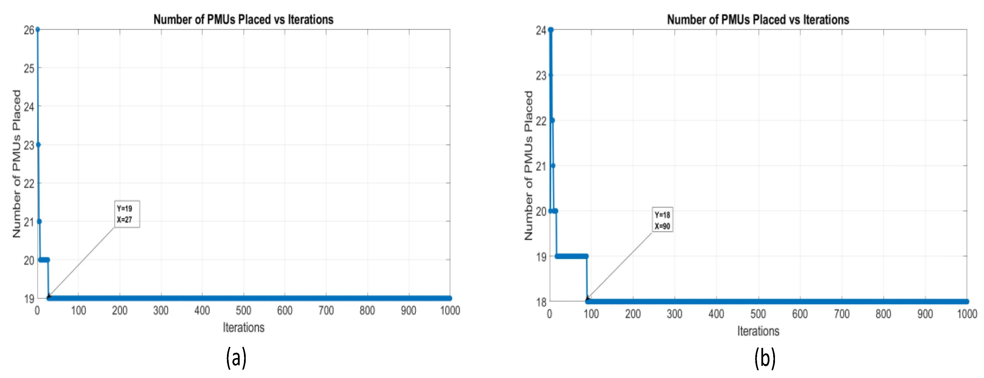
Figure 13.
Voltage Magnitude Estimation for Case Study 1 (a) IEEE 33 bus system PSO&GWO Al-gorithm (b) IEEE 69 Bus System with PSO (c) IEEE 69 Bus System with GWO.
Figure 13.
Voltage Magnitude Estimation for Case Study 1 (a) IEEE 33 bus system PSO&GWO Al-gorithm (b) IEEE 69 Bus System with PSO (c) IEEE 69 Bus System with GWO.
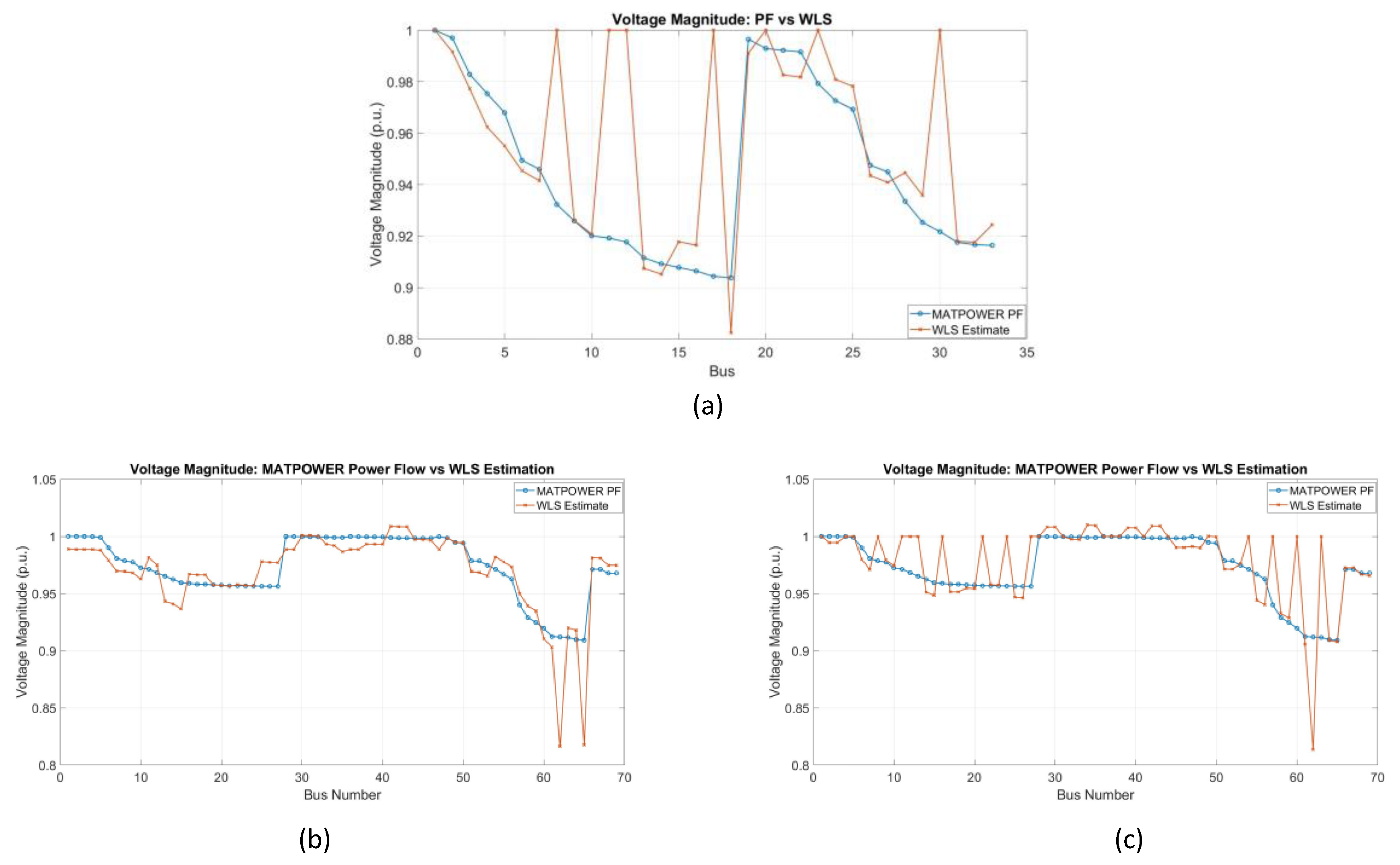
Figure 14.
Voltage Estimation Error for Case Study 1 (a) IEEE 33 bus system PSO&GWO Algorithm (b) IEEE 69 Bus System with PSO (c) IEEE 69 Bus System with GWO.
Figure 14.
Voltage Estimation Error for Case Study 1 (a) IEEE 33 bus system PSO&GWO Algorithm (b) IEEE 69 Bus System with PSO (c) IEEE 69 Bus System with GWO.
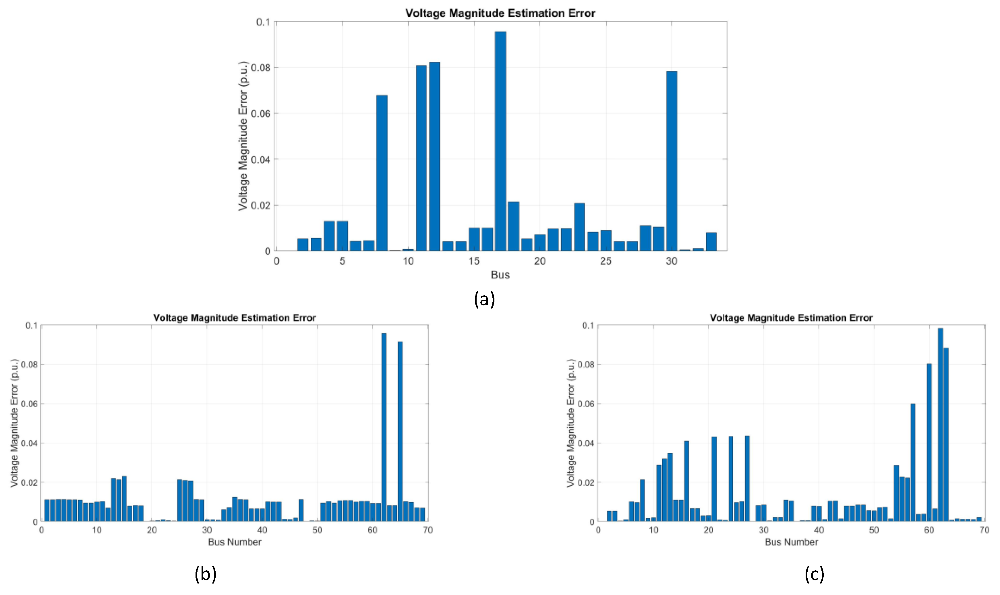
Figure 15.
Voltage Magnitude Estimation for Case Study 2 (a) IEEE 33 bus system with PSO Algorithm (b) IEEE 33 bus system with GWO Algorithm (c) IEEE 69 Bus System with PSO Algorithm (d) IEEE 69 Bus System with GWO Algorithm.
Figure 15.
Voltage Magnitude Estimation for Case Study 2 (a) IEEE 33 bus system with PSO Algorithm (b) IEEE 33 bus system with GWO Algorithm (c) IEEE 69 Bus System with PSO Algorithm (d) IEEE 69 Bus System with GWO Algorithm.
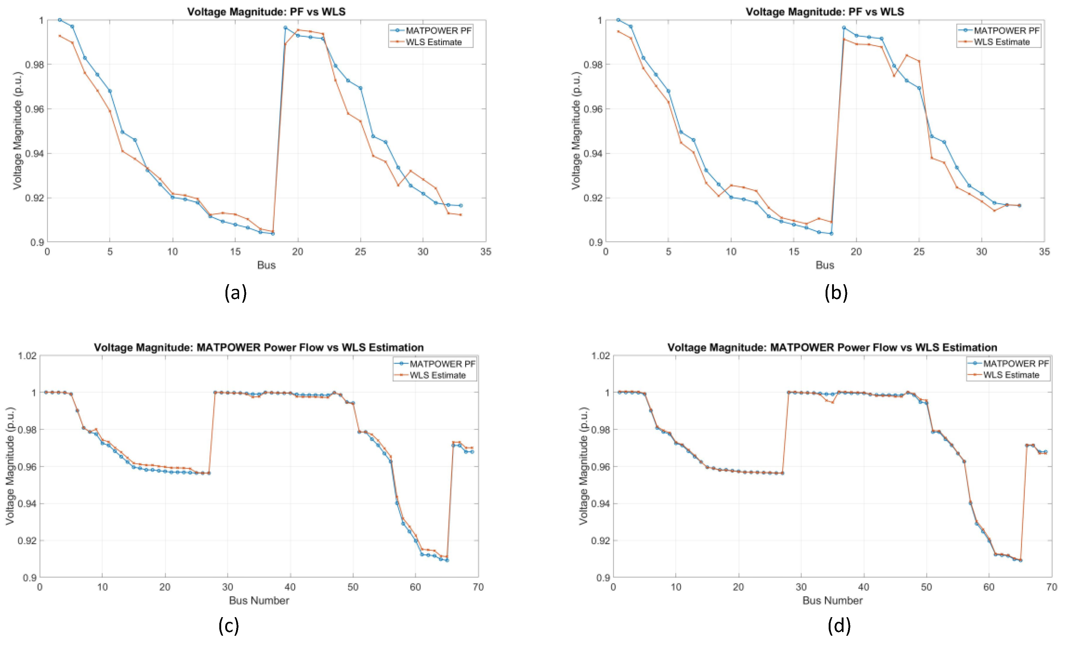
Figure 16.
(a) and (b), (c) and (d).
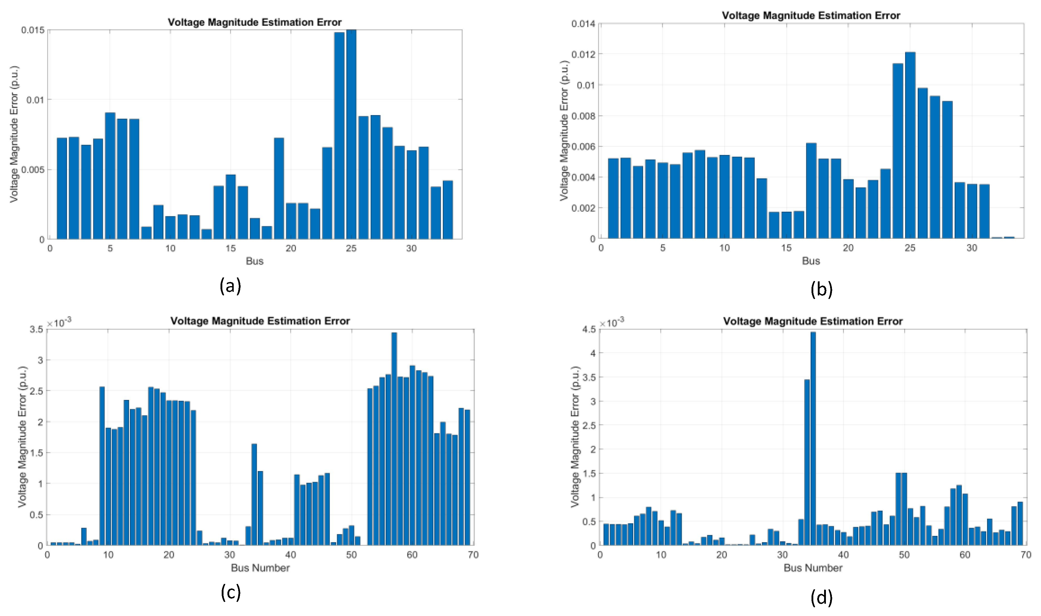
Figure 17.
Voltage Magnitude Estimation for Case Study 3 (a) IEEE 69 Bus System with PSO Algorithm (b) IEEE 69 Bus System with GWO Algorithm.
Figure 17.
Voltage Magnitude Estimation for Case Study 3 (a) IEEE 69 Bus System with PSO Algorithm (b) IEEE 69 Bus System with GWO Algorithm.
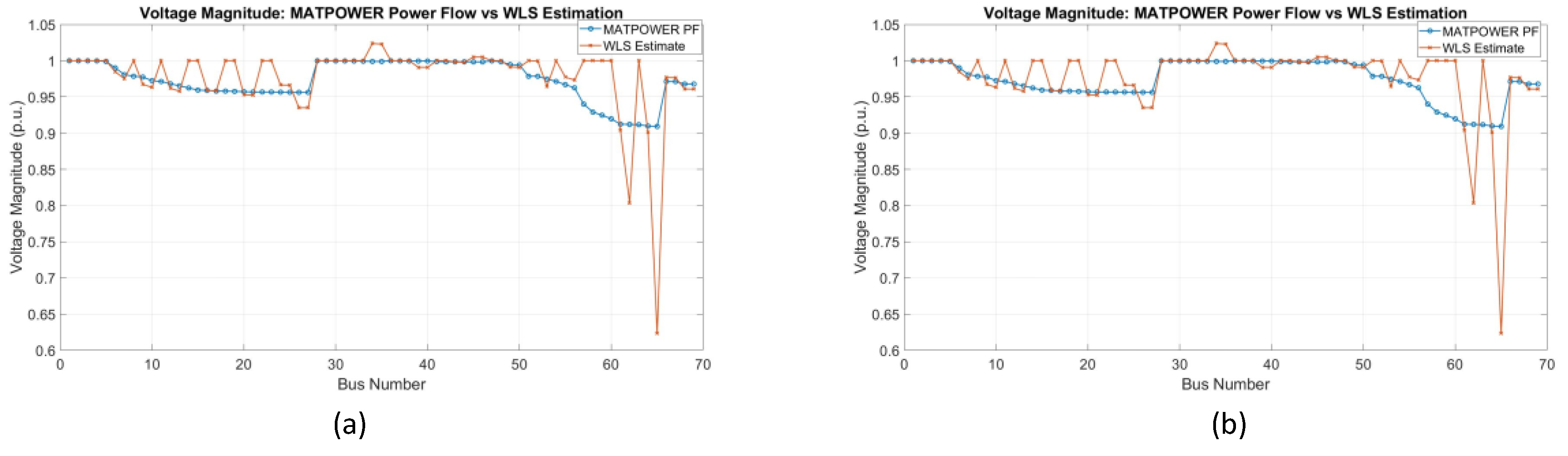
Figure 18.
Voltage Estimation Error for Case Study 3 (a) IEEE 69 Bus System with PSO Algorithm (b) IEEE 69 Bus System with GWO Algorithm.
Figure 18.
Voltage Estimation Error for Case Study 3 (a) IEEE 69 Bus System with PSO Algorithm (b) IEEE 69 Bus System with GWO Algorithm.
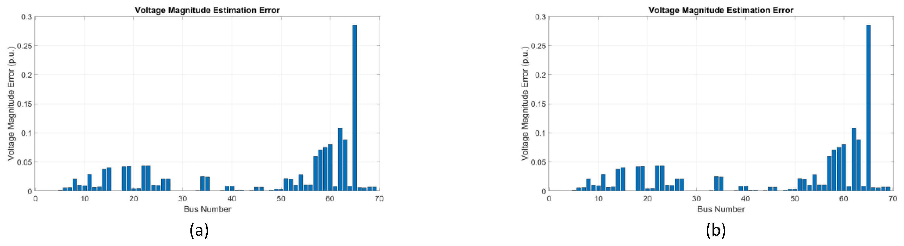
Figure 19.
Voltage Magnitude Estimation for Case Study 1 (a) 0.02 STD in IEEE 33 Bus System with both PSO and GWO Algorithm (b) 0.02 STD in IEEE 69 Bus System with PSO Algorithm (c) 0.02 STD in IEEE 69 Bus System with GWO Algorithm (d) 0.04 STD in IEEE 33 Bus System with both PSO and GWO Algorithm (e) 0.04 STD in IEEE 69 Bus System with PSO Algorithm (f) 0.04 STD in IEEE 69 Bus System with GWO Algorithm.
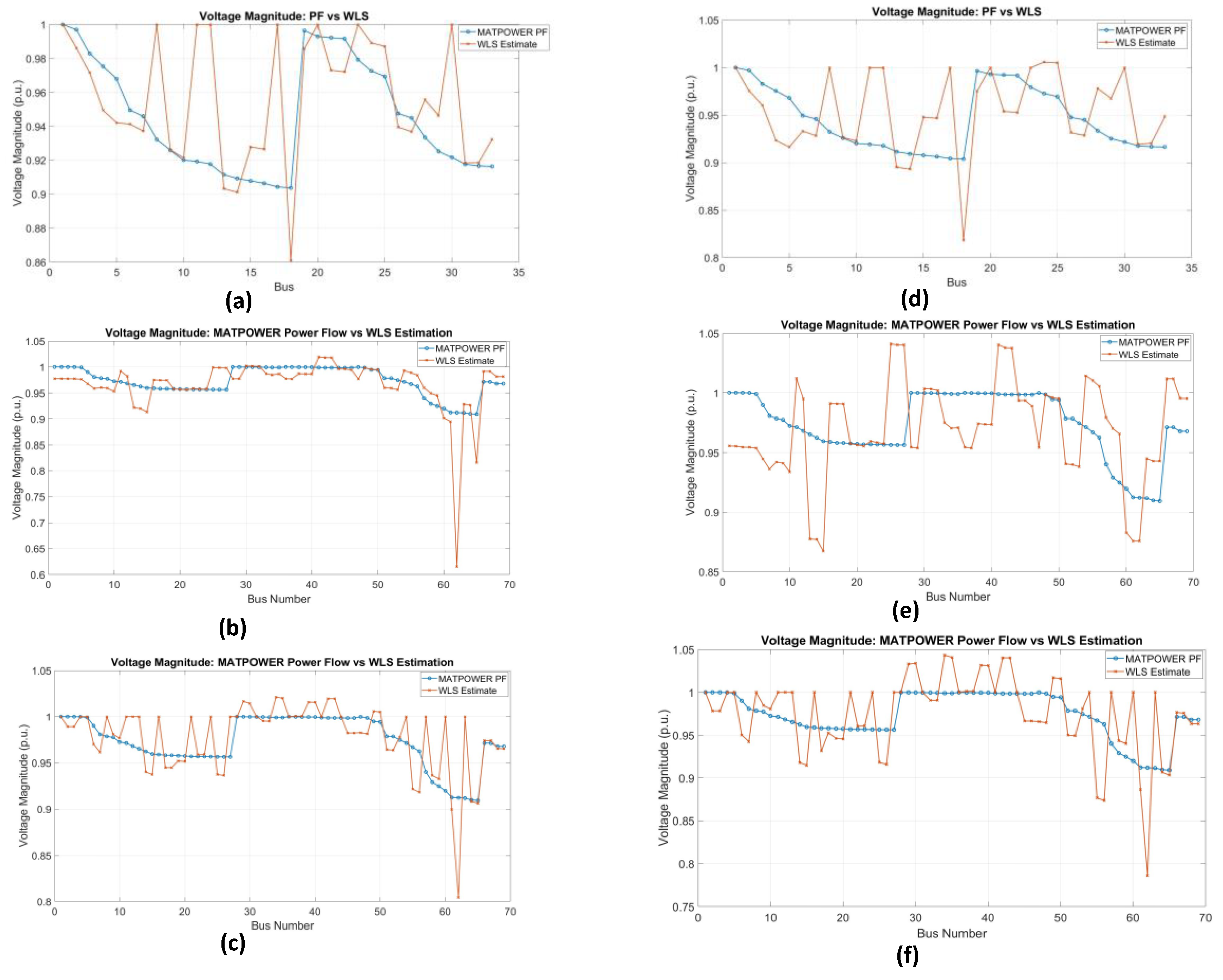
Figure 20.
Voltage Magnitude Estimation for Case Study 2 (a) 0.02 STD in IEEE 33 Bus System PSO Algorithm (b) 0.02 STD in IEEE 33 Bus System with GWO Algorithm (c) 0.04 STD in IEEE 33 Bus System with PSO Algorithm (d) 0.04 STD in IEEE 33 Bus System with GWO Algorithm (e) 0.02 STD in IEEE 69 Bus System with PSO Algorithm (f) 0.02 STD in IEEE 69 Bus System with PSO Algorithm (g) 0.04 STD in IEEE 69 Bus System with PSO Algorithm (h) 0.04 STD in IEEE 69 Bus System with GWO Algorithm.
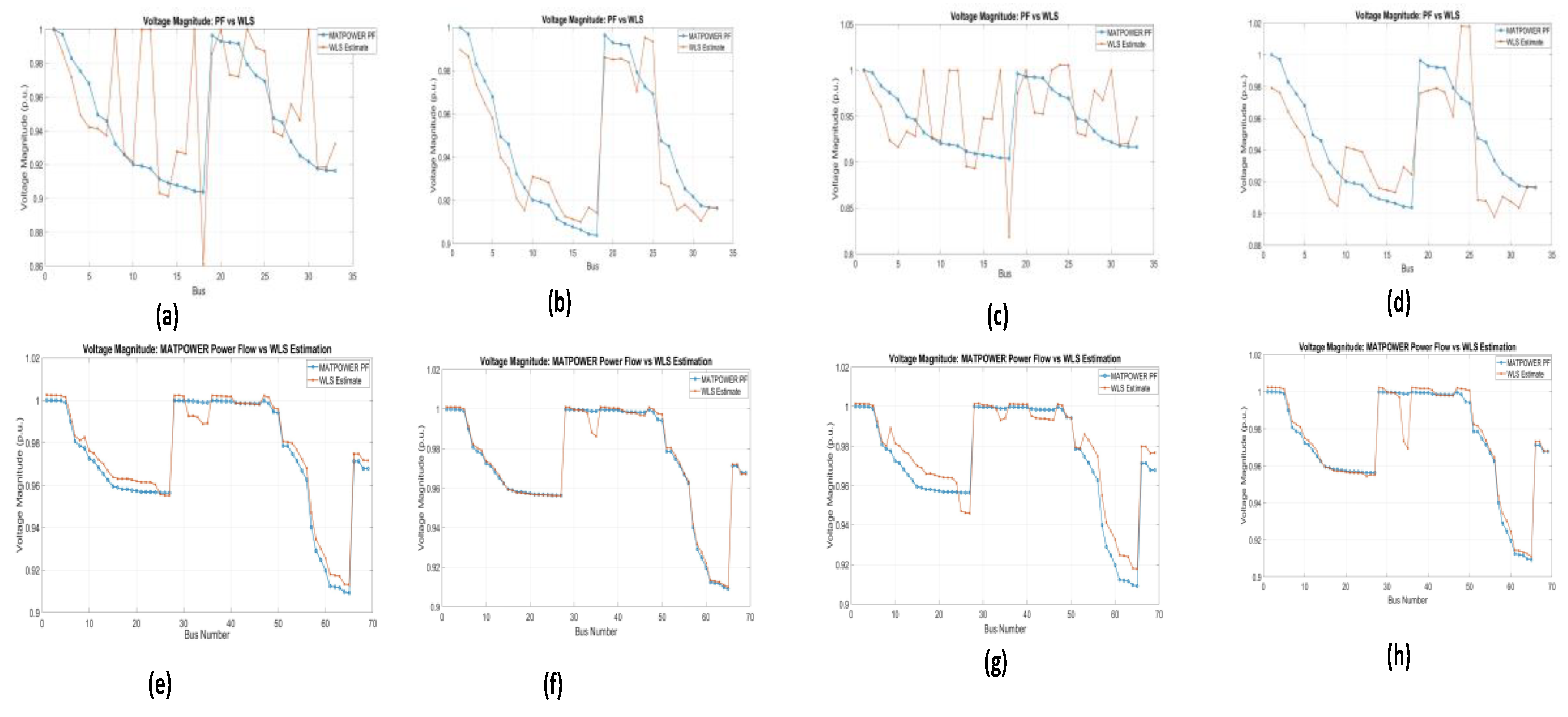
Figure 21.
Voltage Magnitude Estimation for Case Study 3 (a) 0.02 STD in IEEE 69 Bus System PSO Algorithm (b) 0.02 STD in IEEE 69 Bus System with GWO Algorithm (c) 0.04 STD in IEEE 69 Bus System with PSO Algorithm (d) 0.04 STD in IEEE 69 Bus System with GWO Algorithm.
Figure 21.
Voltage Magnitude Estimation for Case Study 3 (a) 0.02 STD in IEEE 69 Bus System PSO Algorithm (b) 0.02 STD in IEEE 69 Bus System with GWO Algorithm (c) 0.04 STD in IEEE 69 Bus System with PSO Algorithm (d) 0.04 STD in IEEE 69 Bus System with GWO Algorithm.
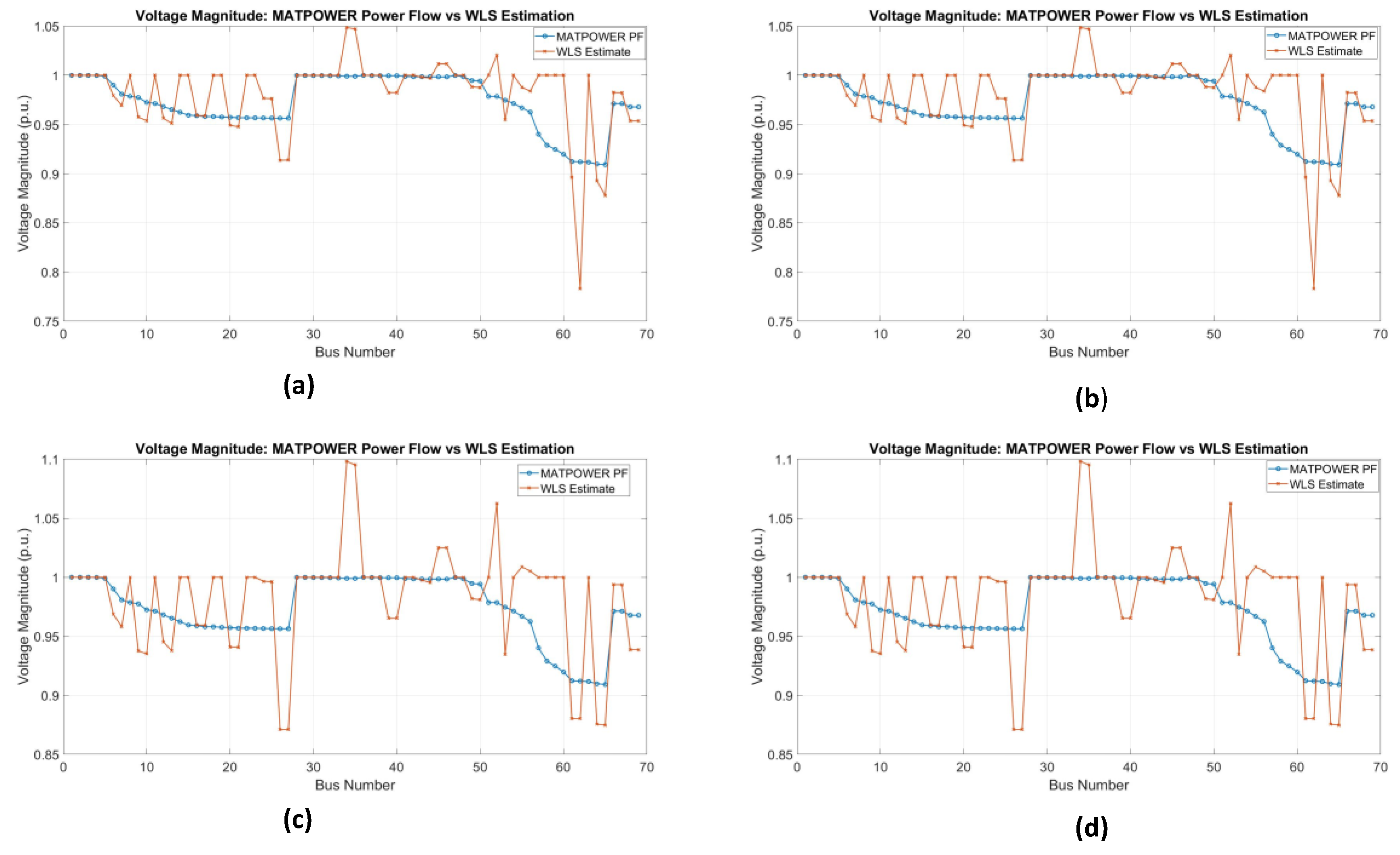

Table 1.
Number of µ-PMUs Placed Under Normal Conditions.
| Techniques | IEEE Bus System | Buses on which µ-PMUs are placed | SORI | Mean of SORI |
|---|---|---|---|---|
|
PSO |
33 |
11 & (2, 4, 8, 11, 14, 17, 21, 24, 26, 29, 32) |
34 |
1.0303 |
|
PSO |
69 |
25 & (2, 4, 6, 9, 14, 17, 20, 23, 26, 28, 31, 34, 36, 39, 42, 45, 49, 51, 55, 58, 61, 64, 66, 68) |
76 |
1.1014 |
| GWO | 33 | 11 & (2, 4, 8, 11, 14, 17, 21, 24, 26, 29, 32) | 34 | 1.0303 |
|
GWO |
69 |
24 & (2, 6, 9, 14, 17,19, 22, 25, 29, 32, 34, 37, 39, 42, 45, 47, 49, 51, 55, 58, 61, 64, 66, 68) |
70 |
1.0145 |
Table 2.
Number of µ-PMUs Placed with A Single PMU Outage.
| Techniques | IEEE bus system | Buses on which µ-PMUs are placed | SORI | Mean of SORI |
|---|---|---|---|---|
|
PSO |
33 |
24 & (1, 2, 3, 5, 6, 8,9, 10, 11, 12, 14, 15, 17, 18, 20, 21, 22, 24, 25, 26, 27, 29, 30, 32, 33) |
70 |
2.1212 |
|
PSO |
69 |
52 & (1, 2, 3, 4, 6, 7, 10, 11, 12, 14, 15, 17, 18, 20, 21, 23, 24, 26, 27, 28, 29, 31, 32, 34, 35, 37, 38, 39, 41, 42, 43, 45, 46, 47, 49, 50, 51, 52, 53, 54, 55, 57, 58, 60, 61, 62, 64, 65, 66, 67, 68, 69) |
152 |
2.2029 |
|
GWO |
33 |
25 & (1, 2, 3, 4, 5, 7, 8, 10, 11, 12, 14, 15, 17, 18, 20, 21, 22, 24, 25, 26, 27, 29, 30, 32, 33) |
72 |
2.1818 |
|
GWO |
69 |
51 & (1, 2, 4, 6, 7, 9, 10, 13, 14, 15, 16, 18, 19, 21, 22, 24, 25, 26, 27, 28, 29, 31, 32, 34, 35, 36, 37, 39, 40, 42, 43, 45, 46, 47, 49, 50, 51, 52, 54, 55, 57, 58, 59, 61, 62, 64, 65, 66, 67, 68, 69) |
146 |
2.1159 |
Table 3.
Number Of µ-PMUs Considering Zero Injection Buses (ZIBs).
| Techniques | IEEE Bus System | Number of ZIBs | Buses on which µ-PMUs are placed | SORI | Mean of SORI |
|---|---|---|---|---|---|
|
PSO |
69 |
20 & (2, 3, 4, 5, 15, 19, 23, 25, 30, 31, 32, 38, 42, 44, 47, 56, 57, 58, 60, 63) | 19 & (6, 9, 12, 16, 20, 24, 26, 34, 39, 43, 45, 49, 52, 55, 61, 64, 66, 68) |
83 |
1.2029 |
|
GWO |
69 |
20 & (2, 3, 4, 5, 15, 19, 23, 25, 30, 31, 32, 38, 42, 44, 47, 56, 57, 58, 60, 63) | 18 & (6, 9, 12, 16, 20, 24, 26, 34, 39, 43, 45, 49, 52, 55, 61, 64, 66, 68) |
77 |
1.115 9 |
Table 4.
Comparative Analysis of PSO & GWO.
| IEEE Test Systems | Case Studies | Nµ-PMUs with PSO | Nµ-PMUs with GWO | [37] MILP |
[9] ILP |
[28] ILP |
[6] ILP |
|---|---|---|---|---|---|---|---|
| 33 | Case 1 | 11 | 11 | 11 | 11 | NR | NR |
| 69 | Case 1 | 25 | 24 | 24 | NR | 24 | 24 |
|
33 |
Case 2 |
25 |
25 |
NR |
NR |
NR |
NR |
| 69 69 |
Case 2 Case 3 |
52 19 |
51 18 |
NR 16 |
NR NR |
NR NR |
NR NR |
| NR means | Not Reported |
Table 5.
Convergence Time for PSO and GWO.
| Case Study | Bus System | Algorithm | Computation Time (seconds) |
|---|---|---|---|
| 1 | 33 | PSO | 1.522581 |
| 1 | 33 | GWO | 2.521862 |
| 1 | 69 | PSO | 577.543879 |
| 1 | 69 | GWO | 212.663388 |
| 2 | 33 | PSO | 1.496152 |
| 2 | 33 | GWO | 1.861462 |
| 2 | 69 | PSO | 3.310082 |
| 2 | 69 | GWO | 5.256499 |
| 3 | 69 | PSO | 4.132528 |
| 3 | 69 | GWO | 19.119925 |
Disclaimer/Publisher’s Note: The statements, opinions and data contained in all publications are solely those of the individual author(s) and contributor(s) and not of MDPI and/or the editor(s). MDPI and/or the editor(s) disclaim responsibility for any injury to people or property resulting from any ideas, methods, instructions or products referred to in the content. |
© 2025 by the authors. Licensee MDPI, Basel, Switzerland. This article is an open access article distributed under the terms and conditions of the Creative Commons Attribution (CC BY) license (http://creativecommons.org/licenses/by/4.0/).
Copyright: This open access article is published under a Creative Commons CC BY 4.0 license, which permit the free download, distribution, and reuse, provided that the author and preprint are cited in any reuse.


