
Submitted:
26 November 2025
Posted:
28 November 2025
You are already at the latest version
Abstract
Groundwater resources management is a critical issue for populations in regions with significant growth. In arid and semiarid regions, where rainfall is scarce, groundwater is often the only source of water for all their needs. Nevertheless, groundwater characterization is virtually unknown in countries with limited infrastructure and resources. A short-term solution is to study groundwater through numerical simulation using the limited available data. We developed a GIS-integrated groundwater flow scheme based on the finite-difference method to numerically simulate a heterogeneous medium using surface geological information. We validate our implementation by comparing it with MODFLOW. We performed groundwater simulations of the Administrative Aquifer in Calera, Zacatecas, Mexico, using homogeneous and heterogeneous media to evaluate flow changes resulting from heterogeneities. We found that numerical simulations show flow barriers in low hydraulic-conductivity zones that coincide with the administrative boundaries of the aquifer; however, in high hydraulic-conductivity zones, the administrative aquifer boundaries do not match the geological limits of the aquifer. This finding gives insight into reconsidering the administrative boundaries of some aquifers in the region for their sustainability, with an integral understanding of groundwater.
Keywords:
groundwater
; modeling
; gis
; finite difference
; administrative aquifer
1. Introduction
Water resources management is a critical issue, particularly in regions where populations are growing. This directly affects the water demand for industrial, agricultural, commercial, and domestic use [1]. This issue is generally addressed without considering environmental implications or presenting sustainable water management, which directly affects regional development.
Recent studies on water availability [2,3] estimate that only % of all the Earth’s water is freshwater, whereas most of it is in the oceans. From the freshwater, nearly 30% is groundwater, 69% is in glaciers and ice caps, and % is in surface water bodies (lakes, rivers, dams, etc.). In arid or semi-arid regions in particular, the greatest availability is in the subsurface. For this reason, groundwater exploitation has increased in Mexico, often with limited knowledge of its features [1]. There are many Mexican cities in semi-arid and arid regions where groundwater constitutes the only drinking water supply [4]. Overall, in Mexico, groundwater comprises almost 40% of the supply, according to the Mexican National Commission on Water [CONAGUA, 5].
Scientific tools have been continually developed within the hydrogeological community [4] to achieve optimal characterization of this vital resource. Such methods involve evaluating groundwater flow directions using chemical and piezometric data, sometimes to determine recharge zones or to analyze the quality of water extracted from the subsoil.
Despite significant contributions in the field of groundwater, there are still regions where water management agencies estimate water budgets using outdated techniques, with limited data, and often without considering a conceptual model that incorporates all the region’s hydrogeological variables [6]. This leads to the misclassification of an administrative aquifer as over-exploited.
Among the elements necessary for the optimal construction of a conceptual hydrogeological model are delineation of the basement, determination of water chemistry, identification of recharge and discharge zones, definition of saturated and unsaturated zones, and determination of subsurface heterogeneities in terms of hydraulic conductivity. For the determination of hydraulic parameters, such as conductivity, analytical techniques have been developed [7] based on ideal solutions that are generally not found in real aquifer scenarios; for example, a homogeneous, infinite-extent aquifer. Numerical techniques for determining this parameter can be statistical or involve a data inversion, which can lead to inadequate models due to the non-uniqueness of inverse problems.
In this work, we developed an integrated scheme that uses geographic information system (GIS) tools to obtain a heterogeneous conductivity model. This scheme was subsequently applied to groundwater modeling to determine the implications for flow systems in a heterogeneous region. Furthermore, a simulation code for confined aquifers was developed that enables direct transition between GIS and groundwater modeling without requiring a graphical interface. This aims to facilitate hydrogeological data inversion with model constraints, based on prior information about surface geology or geophysical data.
This paper is structured into four sections: a description of the study area; an overview of groundwater modeling and GIS integration; groundwater flow results and discussions for homogeneous and heterogeneous media in the Calera Aquifer; and our conclusions.
2. Study Area
The Calera Aquifer is one of the administrative aquifers in the state of Zacatecas established by CONAGUA, which is the Mexican government-dependent organization that manages water in the country. Calera’s boundaries were mainly delimited considering geopolitical factors [5]. It is located on the Mexican Plateau, in the state of Zacatecas, Mexico (Figure 1). Geographically, the aquifer includes 3 of the region’s most populous cities: Zacatecas City (the state’s capital), Fresnillo, and Calera. Within its limits, there is an extensive presence of industrial, mining, commercial, and agricultural activities that, alongside the dense population, make it one of the most studied aquifers in the State. This aquifer’s region is also where we find most of the agricultural activities, predominating irrigation methods by gravity and trickle. Besides, this region is home to one of the most important breweries and one of the most important silver mines in the world.
Most of the research in this aquifer is based on chemical water analyses, from water quality for human consumption [8], water quality for agricultural uses [9], identifying groundwater flow directions [5,10], to determining the presence of recharge zones [11]. Agricultural studies are also available [12], given the extensive use of the soil in the region. However, groundwater modeling studies are scarce. The single study in the region, with 21 piezometric data points, dates back to 1994 [13]; therefore, the data is outdated and unreliable for comparison with modern-day data. Furthermore, geophysical prospecting studies in the region are scarce in the literature. There is a single work that employs Transient-Electromagnetic (TEM) measurements [14], which could lead to a 3D conceptual model in the future.
The main goal of this work is to contribute to the study of water resources in this region by providing a GIS-integrated tool and conceptual models to better understand the aquifer, with the hope of changing the way water is managed in this region and increasing awareness of the water availability problem.
2.1. Hydrogeological background
The Calera aquifer is located in the Sierra Madre Oriental, which is a mountain range in the Mexican Plateau characterized by submarine volcanic and sedimentary deposits. In terms of tectono-stratigraphy, the aquifer lies near the triple junction of the Guerrero Composite, Central, and Oaxaquia Terranes [15], but is mostly within the Central Terrane, where the nature of the basement remains unknown. The geological map in Figure 2 was obtained from shapefiles downloaded from the Mexican Geological Services (SGM).
Regionally, the aquifer presents a horst-graben system [14], with alluvial and lacustrine deposits in the central part of the valley, where almost all well data are located (Figure 2). The sedimentary basin is surrounded at the south by two important geological formations composed of igneous rocks such as Tuff, Rhyolite, and Andesite; the Chilitos Formation [16] at the southwest part of the aquifer and the Zacatecas formation [17] at the southeast, where recharge zones have been identified by isotope analysis [11].
There are no piezometers installed in the region for time-dependent observations, or even for stationary. Usually, all piezometric data are collected with level loggers or conventional water-level meters; hence, there is no information about the well properties in the region. Despite this, water budgets in the aquifer are often performed assuming homogeneous media, without information on the vertical component of flow directions, using simplified groundwater frameworks [7] and, sometimes, a single pumping test experiment with no observation wells.
Static Water Level (SWL) data is available in the CONAGUA databases, which provide a geographical viewer to download piezometric data for a single state and/or administrative aquifer. We downloaded the data within the limits of Figure 2, that is, not only the inner data in the polygon, but also the well data around the aquifer. The database contains sparse information for the years 1996 to 2025, with many missing data points (82.9% are zero). This is due to poorly organized data acquisition campaigns in the region, which occur at irregular intervals and at different well locations.
To estimate the hydraulic head, the well’s surface elevation is needed. For this, we consider the Digital Elevation Model (DEM) of Figure 3 for each data point, then we subtract the elevation from the SWL to obtain the Static Water Elevation (SWE) in meters, as presented in Figure 2, where SWE is shown in the well’s colors. This indicated that groundwater flows from south to north towards the central part of the basin, a hypothesis that will be explored through numerical modeling.
2.2. Digital Elevation Map and Gravity of Calera Aquifer
There are elevation points up to 2700 m.a.s.l. in the aquifer, and lower elevation points on the central part of the basin (2010 m.a.s.l.), as presented on the DEM of Figure 3, obtained from NASA Earthdata free repository. The topography suggests that runoff water flows towards the center of the aquifer, and the recharge zone can be located on the two principal higher parts of the area. The topography is consistent with satellite-gravity data downloaded from the Satellite Geodesy research group at Scripps Institution of Oceanography, at the University of California, San Diego. The higher altitudes in the region, with the higher-density (igneous rocks), produce the highest gravity anomalies on the aquifer. This is an expected feature from a geophysical perspective. There is a negative gravity anomaly in the central part of the medium, where the density is constant (alluvial deposits) and the topography is relatively flat. This could be related to a mass deficit in the medium associated with the presence of extraction wells in the zone (Figure 2); however, at this time, we lack the data to support this hypothesis. Incorporation of additional geophysical information and well logging data is needed.
3. Methodology
3.1. Groundwater Flow Modeling
We consider the partial differential equation for a confined, heterogeneous, and anisotropic aquifer, given by
where is the hydraulic conductivity tensor, is the hydraulic head (m), is the source and/or sink term (s−1), is the specific storage of the porous material (m−1) and t is time (s). For non-orthogonal anisotropy, only the diagonal components of K are considered, therefore, equation (1) can be written as
where , and are the hydraulic conductivities along the x, y and z directions (m/s). Equation 2 is the main equation for groundwater modeling, and can be solved using Finite Difference Methods [FDM, 18] or Finite Element Methods [FEM, 19]; in this paper, we only consider FDM. The discretization of Equation 2 yields the following ODE system
where is hydraulic head (vectorized), is the vector containing all the source-sink terms, and and are matrices obtained from the application of the stencil on the grid (see Appendix A), and include the hydraulic conductivity, specific storage, and boundary conditions [20]. We solve the matrix system of Equation 3 using Biconjugate Gradient Stabilized Method (BiCGSTAB) [21] for the non-symmetric problem.
In practice, the transient-state model (Equation 3) requires time stepping, which can be performed using implicit or explicit methods [22]. To realistically model a transient-state problem, data must be recorded over several time periods, sometimes in logarithmic increments from seconds to days, or from days to years, in well-known piezometric networks, sometimes requiring in situ pumping test data acquisition [7]. Nevertheless, in the Calera aquifer, there are regions where a well datum, i.e., Static Water Level (SWL), is used instead of piezometric monitoring, with data collected every 5 years. Additionally, the z-component information (well screen and casing depths) is never provided. With respect to pumping test data, in our area of study, there is sometimes no observation well for the experiment, leading to measurement errors, and most of the time, only a single pumping test is performed across the entire aquifer region for water budget evaluations. Given the limited data availability, we limit our study to 2D steady-state modeling; hence, equation 2 can be simplified as
Although our implementation is designed for 3D, anisotropic, and steady-state modeling, the 2D simulation is straightforward (see Appendix A).
3.2. Conductivity Model Creation
For the conductivity model, we used the geology of the area of interest (Figure 2), where alluvial deposits are most prevalent in the zone, and volcanic structures surround the southern part of the region. To obtain a conductivity model, Geographical Information System software is needed, such as ArcGIS [23] or QGIS [24]. An alternative for GUI software is Geopandas [25], which has recently become popular among code developers to avoid graphical interfaces [26]. Geopandas is an open-source Python 3 project that manipulates dataframes similarly to the Pandas package, with spatial operations on geometry types (points and polygons). This feature allows us to create a dataframe column with hydraulic conductivity values depending on the rock type in the zone. For this, we take the mean of the range of values of Bear [27] to obtain the hydraulic conductivities presented in Table 1.
We consider mainly 3 hydrogeological environments in our region of study: 1) a high hydraulic conductivity zone for sedimentary deposits (Alluvial and Lacustrine deposits), 2) an intermediate hydraulic conductivity zone for conglomerate, sandstone, and limestone, and 3) a low conductivity region for igneous rocks(mostly rhyolite and andesite) and shale. All zones are based on the mean values of the ranges presented by Bear [27] (see Figure 4a).
The alluvial region consists predominantly of coarse- to medium-grained sands, hence the high-conductivity values. For lacustrine, we set high conductivity values because this is the region where dry lakes and rivers occur in the Calera aquifer. For the intermediate zone, we chose a value that accounts for poor cementation and high porosity. Finally, igneous and non-fractured rocks yielded the lowest conductivity. However, fractured igneous rocks could have conductivities comparable to those of gravel deposits. This would require in situ cartography of faults or fractures in the region, or geophysical data acquisition and processing, such as aeromagnetic or seismic data, to identify fractured rocks. We only consider in this work non-fractured rocks, but the model creation could be easily updated in our workflow if more information becomes available.
To determine the grid resolution, we examine piezometric data in the zone. To change to metric units, we transform the coordinates to WGS 84 Zone UTM 13N. Then, we compute the minimal distance among all well data points in the aquifer, which is 273.31 meters. Using a resolution of 250 meters yields a grid size of , which we considered low-resolution compared with the geology map in Figure 2. Besides, the minimal distance would ignore effects between adjacent wells. For this reason, a resolution of 100 meters was chosen, i.e., at least 1 cell will be computed between piezometric data points. This resolution leads to a grid size of , which is negligible for our computational resources.
We wrote Python code using the Geopandas package to transform the GIS file into a grid matrix (), using the hydraulic conductivity values from Table 1 and an external CSV file. The model obtained using this method is presented in Figure 4b, and resembles the geology in the zone. This implementation provides a fast, accessible way to update the hydraulic conductivity value if additional information becomes available, such as well logging, geophysical inversion, in situ cartography, or even groundwater inverse modeling for K estimation [28]. The same procedure, with the same grid size, was performed to compute the head-constant matrix where the wells are located, to feed the FDM code.
4. Results and discussions
Here, we present the results from 3 experiments: first, we test our implementation on a simple 2D homogeneous model for isotropic and anisotropic media, comparing the results with those of MODFLOW. Second, we simulate groundwater flow in the Calera Aquifer using a homogeneous conductivity model and compare the results with those from MODFLOW. Finally, we test our GIS-integrated groundwater model using FDM, accounting for heterogeneous conductivity.
4.1. Validation of our scheme
The main purpose of this experiment is to validate our FDM implementation by comparing it with simulations using MODFLOW 6 [29,30] for isotropic and anisotropic media with different grid sizes (Figure 5). The 2D domains of the following tests are m and m. For boundary conditions, we set a head-constant value m for , and a discharge rate m3/day in the center of the domain, hence the source term is
In MODFLOW, the boundary conditions are implemented with the CHD package and the sink/source implementation with the WEL package [18]. Since we use a steady-state problem, the time units do not play an important role in the simulations; hence, we set the hydraulic conductivities to m/day. For a grid size of , the results for a homogeneous medium are almost the same using MODFLOW (Figure 5a) and our implementation (Figure 5b), where the contours present hydraulic conductivity circles centered at and . The differences between simulations are negligible, as seen in the percentage error in Figure 5c.
Then, we simulate for an anisotropic medium with m/day and m/day, with the same grid size and boundary conditions. Again, the results are similar using MODFLOW (Figure 5d) and our implementation (Figure 5e). In this example, the head contours clearly exhibit the hydraulic conductivity ellipsoid for an anisotropic medium, as presented by Cherry and Freeze [31], i.e., there is faster convergence to the drawdown point in the center along the y-direction than along the x-direction. The percentage error, Figure 5f, is still negligible (up to %).
Finally, we calibrate our code with a larger grid, , for the same anisotropic media. Because of the higher resolution, the head contours are smoother than in the lower-resolution examples (see Figure 5g and Figure 5h). Although the percentage errors are larger than in the low-resolution examples, they are still negligible (Figure 5i).
We present horizontal and vertical profiles of the head for the anisotropic case, using both lower- and higher-resolution simulations for a more detailed comparison. As shown in Figure 6, the results are indistinguishable. These profiles are not to be compared with pumping-test data, because they are for a steady-state regime and do not account for infinite boundaries [7].
4.2. Calera Aquifer groundwater modeling for homogeneous medium
We performed steady-state groundwater modeling of the administrative aquifer in Calera, Zacatecas, Mexico (Figure 1), using the piezometric information from Figure 2 (Static Water Height) and a homogeneous hydraulic conductivity model with m/day. This consideration allows us to compare the experiment with MODFLOW, where homogeneous media is straightforward to implement. Mathematically and numerically, this setup is a Poisson problem; see Equation 2. We set the known piezometric data as the head-fixed value and applied no-flow boundary conditions on the boundaries in our code and in MODFLOW (using the CHD package).
We present the groundwater results in Figure 7, using a grid of . As in the previous experiment, the results are very similar for both methodologies, showing flow from the center region of the aquifer towards the northeast and southwest regions.
The flow towards NE (inner contour level of 2010 meters) is due to the presence of the deepest water static levels in the region (around 2000 meters). It is consistent with the topography and the gravity anomaly of Figure 3. The flow towards the southwestern part of the model is due to the interaction with the wells in that region (approximately at 22°45’ N and 103°W) for the contour levels 2130 m and outer 2100 m. The simulation results present the highest head value at 23°N and 102.48°W (approximately) on the aquifer, which will be interpreted in the following subsection.
4.3. Calera Aquifer Modeling Heterogeneous Media
With the final calibration of our code, we proceeded to perform groundwater modeling for a heterogeneous medium, taking the hydraulic conductivity model of Figure 4b, based on Table 1. Changing the table values would not require changes to our implementation; hence, it can be easily modified for future work.
Before performing the numerical simulation, we note a head anomaly in the central part of the region in the homogeneous result. This could be interpreted as a point source in the media, such as a recharge zone. However, this finding is not consistent with the topography or previous studies [5,11] in the region. For this reason, we perform an exploratory data analysis of the piezometric information using a box plot, as shown in Figure 8. The box plot presents a single outlier in the CONAGUA database. Since we can not assess the veracity of this outlier (it could be a measurement error or a spring well), we decided to eliminate this datum from the piezometric database.
Then, we perform the modeling using our GIS-integrated code, as shown in the map in Figure 9a, for 2D heterogeneous media. To clarify, we do not set any cells to be inactive in our model; the simulation naturally shows inactive zones in the gray areas, where an umbral NaN is imposed for . This inactive area corresponds to regions with the lowest hydraulic conductivity values (Figure 4), which are associated with non-fractured igneous rocks and shale, especially in the southern part of the model.
We consider this result the most important in our simulation, since geology provides natural limits for an aquifer, which should be necessary to define its administrative delimitation, but this is not always the case.
Hence, geology, through appropriate hydraulic-conductivity models, provides non-interaction zones where wells are separated by low h values, such as the region in the southwest part of the model, which is separated by tuff rocks. In this case, the numerical limit of the aquifer agrees with the administrative one, in combination with the low conductivity of the andesite rocks (southeast). These findings highlight the importance of using heterogeneous rather than homogeneous media in aquifer characterization, as the homogeneous simulation (Figure 7) shows groundwater interactions in zones where, in reality, there are none. On the other hand, in the northern part of the model, there is no numerical barrier in the simulation, which we interpret as a continuity of the geological aquifer outside the administrative aquifer of Calera.
With respect to the lowest contour values of head in the simulation, there is a drawdown zone in the north-center part of the domain, as mentioned in literature on the region and consistent with the mass deficit presented in the gravity anomaly of Figure 3b. This persistent result could support the hypothesis of Bredehoeft [6] that the aquifer is in an equilibrium state; however, z-component information is needed to ascertain this.
5. Conclusions
We developed a FDM groundwater modeling scheme to simulate flow in realistic aquifers. The FDM code was validated by comparing results with those of MODFLOW 6 for simple, homogeneous, and heterogeneous examples with different grid sizes. The scheme is integrated with GIS and provides a quick tool for creating hydraulic conductivity models based on surface outcropping geology, generating grid-sized, heterogeneous models tailored to simulation needs. The main goal of this work was to evaluate groundwater flow patterns in the Calera Aquifer. Using a homogeneous medium, numerical flow simulations can lead to an erroneous interpretation of groundwater movement in the subsoil, which is frequently the case in water-budget evaluations in this area by water-management organizations; namely, homogeneous, 1D, and full-horizontal flow are assumed. When heterogeneities are considered, the flows are more consistent with the geology and piezometry, yielding results similar to those of hydrogeochemical and hydraulic works in the area. In low hydraulic zones, the simulations show numerical flow barriers corresponding to igneous rocks, consistent with the aquifer’s administrative boundary. On the other hand, in high hydraulic-conductivity zones, groundwater interactions are evident in piezometric data outside the aquifer’s administrative limits. We conclude that, geologically speaking, the aquifer does not match the boundaries set by the water organism, which considers only geopolitical factors. We recommend implementing our methodology to define these boundaries to better understand groundwater in the region and to use this vital resource more sustainably. Current limitations arise in the quality and availability of the piezometric data. There are no piezometers in the region, where hydrogeological vertical information is often missing. Even though the code is written for 3D transient, anisotropic, and heterogeneous media, the lack of data constrains us from running more realistic simulations. An important issue is incorporating faults and fractures into the model, which we leave for future work. Also, it is imperative to incorporate additional geophysical data to develop a 3D conceptual model and to perform groundwater modeling that accounts for the vertical component.
Author Contributions
Raúl Ulices Silva-Ávalos developed and tested the GIS integrated algorithm, remodeled and validated according to comments by Hugo Enrique Júnez-Ferreira, who also helped in the composition of the paper. Julian conceived the idea of the problem of groundwater management in the region. Jonas D. De Basabe contributed to the discussions on the Finite Difference implementation and the writing of the manuscript. Luis Gerardo Ortiz-Acuña provided the satellite gravity data in the region, including the processing and the discussions related to the topic. All authors have read and agreed to the published version of the manuscript.
Funding
Not applicable.
Institutional Review Board Statement
Not applicable.
Data Availability Statement
All the data can be downloaded from references within the document, as marked as hyperlinks.
Acknowledgments
Not applicable.
Conflicts of Interest
The authors declare no conflicts of interest.
Abbreviations
The following abbreviations are used in this manuscript:
| MODFLOW | Modular hydrologic flow model |
| FDM | Finite Difference Method |
| DEM | Digital Elevation Model |
| GIS | Geographic Information System |
| CONAGUA | Mexican National Water Commission |
| SWL | Static Water Level |
| SWE | Static Water Elevation |
Appendix A. The Finite Diffence Method
Appendix A.1.
In this appendix, we describe our Finite Difference implementation for a general 3D groundwater flow problem in a heterogeneous, anisotropic medium, in steady state. First, we expand the derivatives in Equation 2 as follows
renaming and , and similarly for x, y, and z, we get
Now, we applied the centered discretization following Spitzer [32], using
where is the grid spacing for the direction. The FD expression for y and z can be easily applied using or for j- or k-indexes, respectively. Equation A3 is also applied to the derivatives , , and from above. Thus, equation (A1) is rewritten as
Arranging the seven terms and applying the FDM to the time derivative, i.e., an implicit formulation, this leads to
where is the previous hydraulic head field, is the time step and is the source term for each t-time. Renaming the coefficients which multiply the terms,
where the letters in the stencil stand for Left, Right, Back, Front, Down, Up, and Center, respectively. thus
and
This discretization results in a system of equations to be solved in the form,
we use Biconjugate Gradient Stabilized Method (BiCGSTAB) [21] for the non symmetrical solution of Equation A8, combinend with large-sparse system storage.
References
- Giordano, M. Global groundwater? Issues and solutions. Annual review of Environment and Resources 2009, 34, 153–178.
- Igor, S. World fresh water resources. Water in crisis: a guide to the world’s. Oxford University Press, Inc, Oxford 1993.
- Sophocleous, M. Global and regional water availability and demand: prospects for the future. Natural Resources Research 2004, 13, 61–75.
- Kinzelbach, W.; Bauer, P.; Siegfried, T.; Brunner, P. Sustainable groundwater management—problems and scientific tools. Episodes Journal of International Geoscience 2003, 26, 279–284.
- Navarro-Solis, O.; González Trinidad, J.; Junez-Ferreira, H.; Cardona, A.; Bautista Capetillo, C. Integrative methodology for the identification of groundwater flow patterns: Application in a semi-arid region of Mexico. Appl. Ecol. Environ. Res 2016, 14, 645–666.
- Bredehoeft, J.D. The Water Budget Myth Revisited: Why Hydrogeologists Model. Groundwater 2002, 40, 340–345, [https://ngwa.onlinelibrary.wiley.com/doi/pdf/10.1111/j.1745-6584.2002.tb02511.x]. [CrossRef]
- Theis, C.V. The relation between the lowering of the Piezometric surface and the rate and duration of discharge of a well using ground-water storage. Eos, Transactions American Geophysical Union 1935, 16, 519–524, [https://agupubs.onlinelibrary.wiley.com/doi/pdf/10.1029/TR016i002p00519]. [CrossRef]
- Navarro, O.; González, J.; Júnez-Ferreira, H.; Bautista, C.F.; Cardona, A. Correlation of arsenic and fluoride in the groundwater for human consumption in a semiarid region of Mexico. Procedia Engineering 2017, 186, 333–340.
- Carrillo-Martinez, C.J.; Álvarez-Fuentes, G.; Aguilar-Benitez, G.; Can-Chulím, Á.; Pinedo-Escobar, J.A. Water quality for agricultural irrigation in the Calera aquifer region in Zacatecas, Mexico. Tecnología y ciencias del agua 2021, 12, 1–58.
- Rivera Armendariz, C.A.; Banning, A.; Cardona Benavides, A. Geochemical evolution along regional groundwater flow in a semi-arid closed basin using a multi-tracing approach. Journal of Hydrology 2024, 632, 130895. [CrossRef]
- González-Trinidad, J.; Pacheco-Guerrero, A.; Júnez-Ferreira, H.; Bautista-Capetillo, C.; Hernández-Antonio, A. Identifying groundwater recharge sites through environmental stable isotopes in an alluvial aquifer. Water 2017, 9, 569.
- Garbrecht, J.; Mojarro, F.; Echavarria-Chairez, F.; Bautista-Capetillo, C.; Brauer, D.; Steiner, J. Sustainable utilization of the Calera aquifer, Zacatecas, Mexico. Applied Engineering in Agriculture 2013, 29, 67–75.
- Hernández, J.E.; Gowda, P.H.; Howell, T.A.; Steiner, J.L.; Mojarro, F.; Núñez, E.P.; Avila, J.R. Modeling Groundwater levels on the Calera aquifer region in central Mexico using ModFlow. Journal of Agricultural Science and Technology B 2012.
- Krienen, L.; Cardona Benavides, A.; Lopez Loera, H.; Rüde, T.R. Understanding deep groundwater flow systems to contribute to a sustainable use of the water resource in the Mexican Altiplano. Technical report, Lehr-und Forschungsgebiet Hydrogeologie, 2019.
- Centeno-García, E.; Guerrero-Suastegui, M.; Talavera-Mendoza, O., The Guerrero Composite Terrane of western Mexico: Collision and subsequent rifting in a supra-subduction zone; 2008; Vol. 436, pp. 279–308. [CrossRef]
- de Cserna, Z. Geology of the Fresnillo area, Zacatecas, Mexico. Geological Society of America Bulletin 1976, 87, 1191–1199.
- Bartolini, C.; Lang, H.; Cantú Chapa, A.; Barboza-Gudiño, R. The Triassic Zacatecas Formation in Central Mexico: Paleotectonic, paleogeo- graphic and paleobiogeographic implications. AAPG Memoir 2001, 75, 295–315.
- Harbaugh, A.W. MODFLOW-2005, the US Geological Survey modular ground-water model: the ground-water flow process; Vol. 6, US Department of the Interior, US Geological Survey Reston, VA, USA, 2005.
- Diersch, H.J.G. FEFLOW: finite element modeling of flow, mass and heat transport in porous and fractured media; Springer Science & Business Media, 2013.
- Asher, M.J.; Croke, B.F.W.; Jakeman, A.J.; Peeters, L.J.M. A review of surrogate models and their application to groundwater modeling. Water Resources Research 2015, 51, 5957–5973, [https://agupubs.onlinelibrary.wiley.com/doi/pdf/10.1002/2015WR016967]. [CrossRef]
- van der Vorst, H.A. Bi-CGSTAB: A Fast and Smoothly Converging Variant of Bi-CG for the Solution of Nonsymmetric Linear Systems. SIAM Journal on Scientific and Statistical Computing 1992, 13, 631–644, [https://doi.org/10.1137/0913035]. [CrossRef]
- Dou, C.; Woldt, W.; Bogardi, I.; Dahab, M. Steady state groundwater flow simulation with imprecise parameters. Water Resources Research 1995, 31, 2709–2719.
- Environmental Systems Research Institute (ESRI). ArcGIS Release 10.1. Redlands, CA, 2012.
- QGIS Development Team. QGIS Geographic Information System. Open Source Geospatial Foundation, 2009.
- Jordahl, K.; den Bossche, J.V.; Fleischmann, M.; Wasserman, J.; McBride, J.; Gerard, J.; Tratner, J.; Perry, M.; Badaracco, A.G.; Farmer, C.; et al. geopandas/geopandas: v0.8.1, 2020. [CrossRef]
- Pulla, S.T.; Yasarer, H.; Yarbrough, L.D. GRACE downscaler: A framework to develop and evaluate downscaling models for GRACE. Remote Sensing 2023, 15, 2247.
- Bear, J. Dynamics of fluids in porous media; Courier Corporation, 2013.
- Poeter, E.P.; Hill, M.C. Inverse models: A necessary next step in ground-water modeling. Groundwater 1997, 35, 250–260.
- Hughes, J.D.; Langevin, C.D.; Banta, E.R. Documentation for the MODFLOW 6 framework. Technical report, US Geological Survey, 2017.
- Langevin, C.D.; Hughes, J.D.; Banta, E.R.; Niswonger, R.G.; Panday, S.; Provost, A.M. Documentation for the MODFLOW 6 groundwater flow model. Technical report, US Geological Survey, 2017.
- Cherry, J.A.; Freeze, R.A. Groundwater; Vol. 370, Englewood Cliffs, NJ: Prentice-Hall, 1979.
- Spitzer, K. A 3-D finite-difference algorithm for DC resistivity modelling using conjugate gradient methods. Geophysical Journal International 1995, 123, 903–914, [https://academic.oup.com/gji/article-pdf/123/3/903/2351337/123-3-903.pdf]. [CrossRef]
Figure 1.
Calera administrative aquifer in Zacatecas, Mexico.
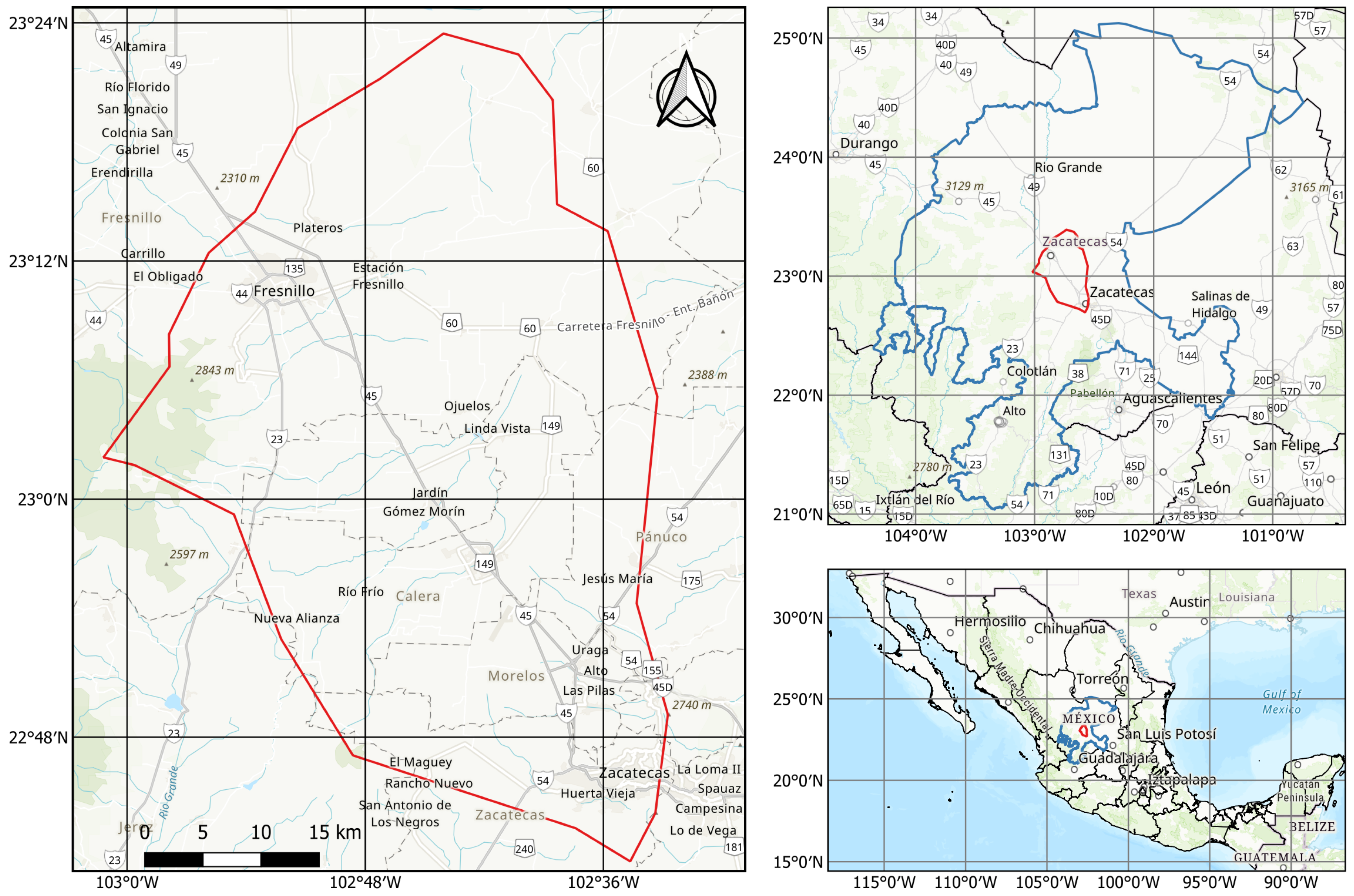
Figure 2.
Geology of the Calera Aquifer and piezometric data (black outlined and blue circles) within the area of study.
Figure 2.
Geology of the Calera Aquifer and piezometric data (black outlined and blue circles) within the area of study.
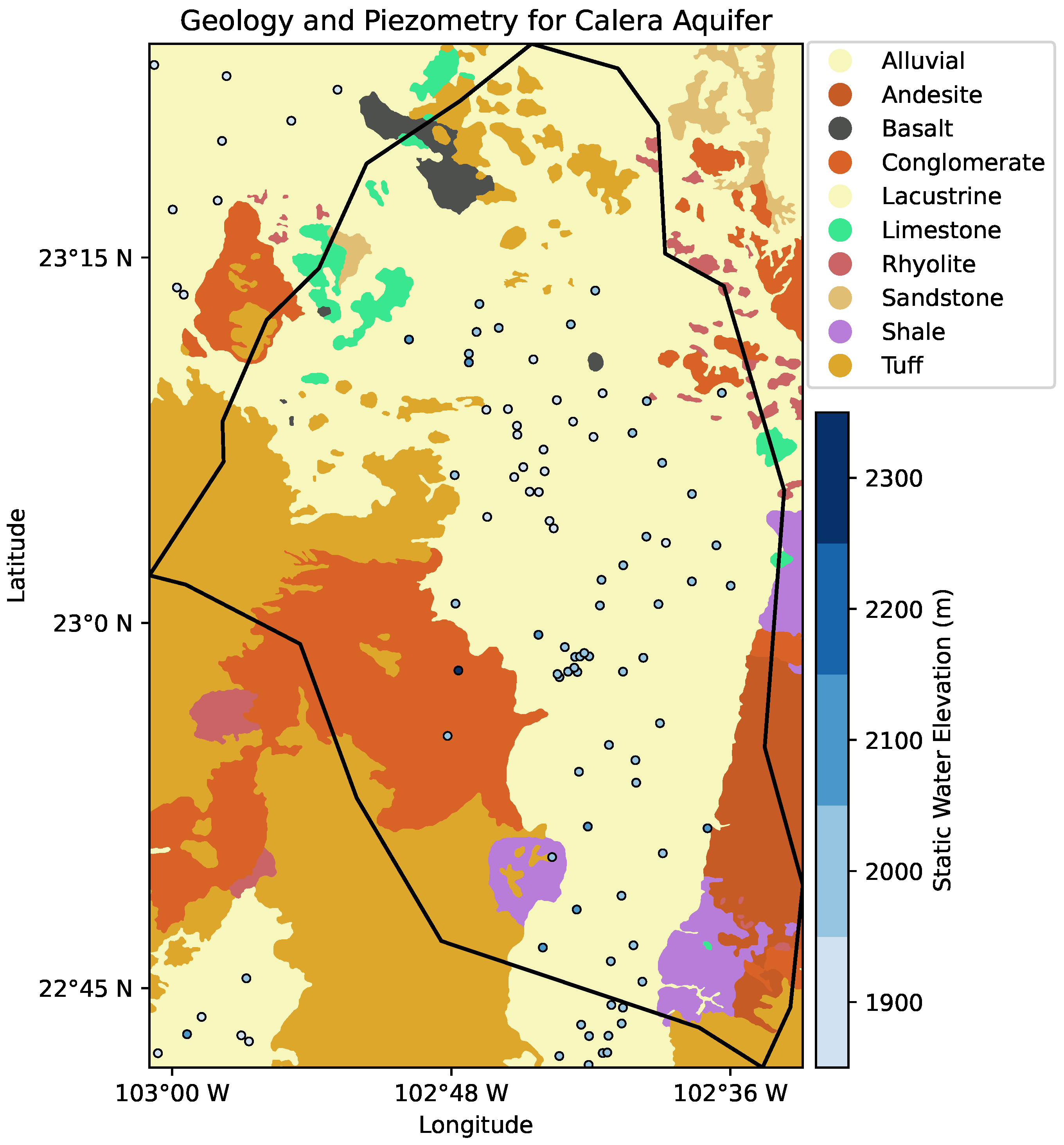
Figure 3.
a) Digital Elevation Model and b) Satellite Gravity Data for the Calera aquifer
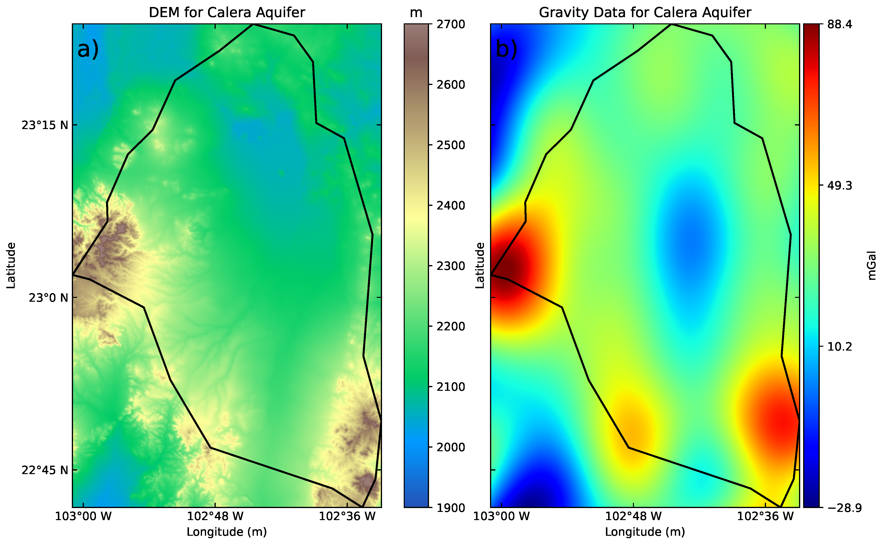
Figure 4.
a) Hydraulic conductivity GIS using the values of Table 1 and b) Hydraulic Conductivity model () using a resolution of 100 meters.
Figure 4.
a) Hydraulic conductivity GIS using the values of Table 1 and b) Hydraulic Conductivity model () using a resolution of 100 meters.
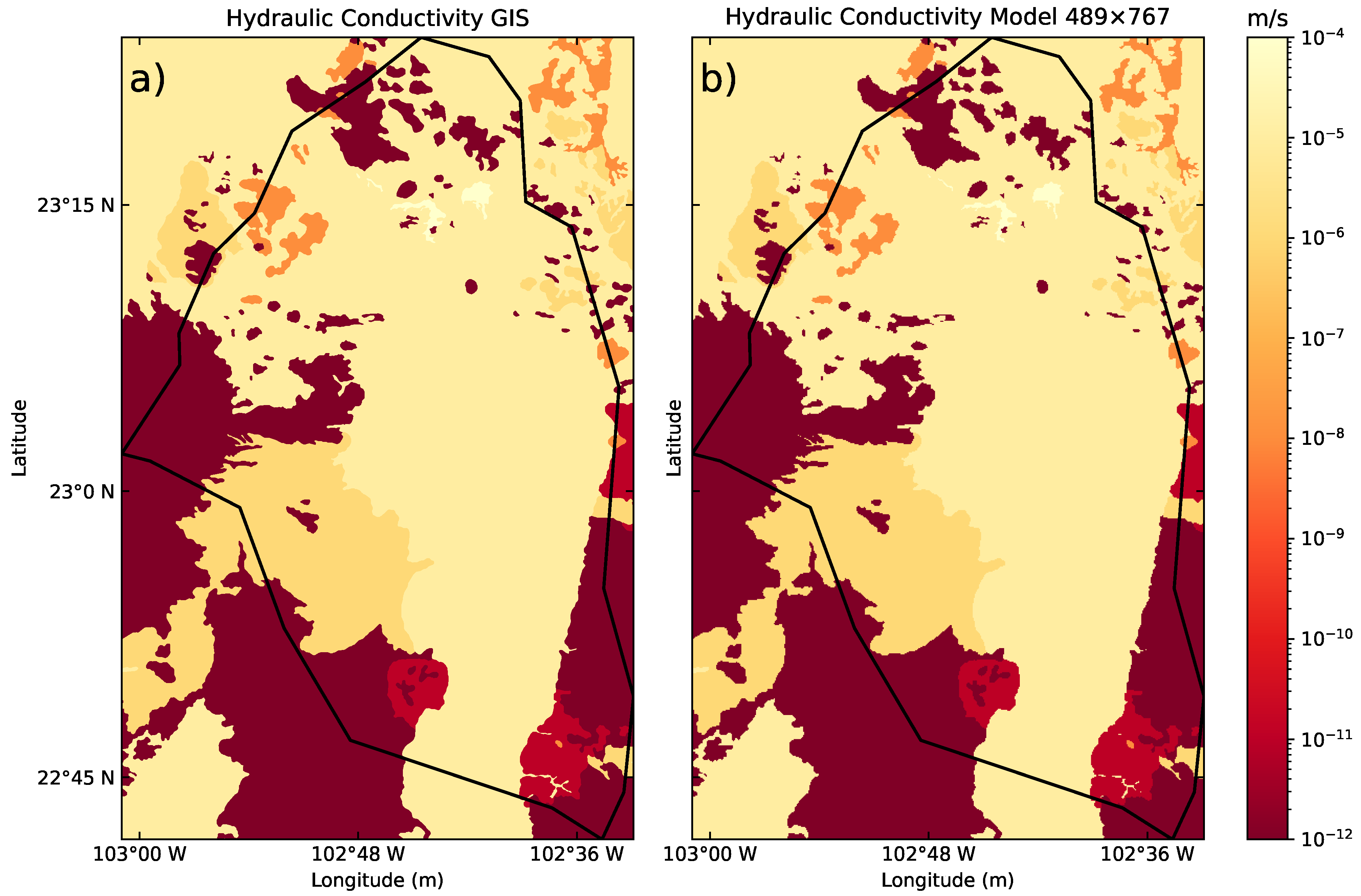
Figure 5.
Numerical head simulation comparing our FDM results with those of MODFLOW for homogeneous media, using isotropic and anisotropic hydraulic conductivity for different grid sizes.
Figure 5.
Numerical head simulation comparing our FDM results with those of MODFLOW for homogeneous media, using isotropic and anisotropic hydraulic conductivity for different grid sizes.
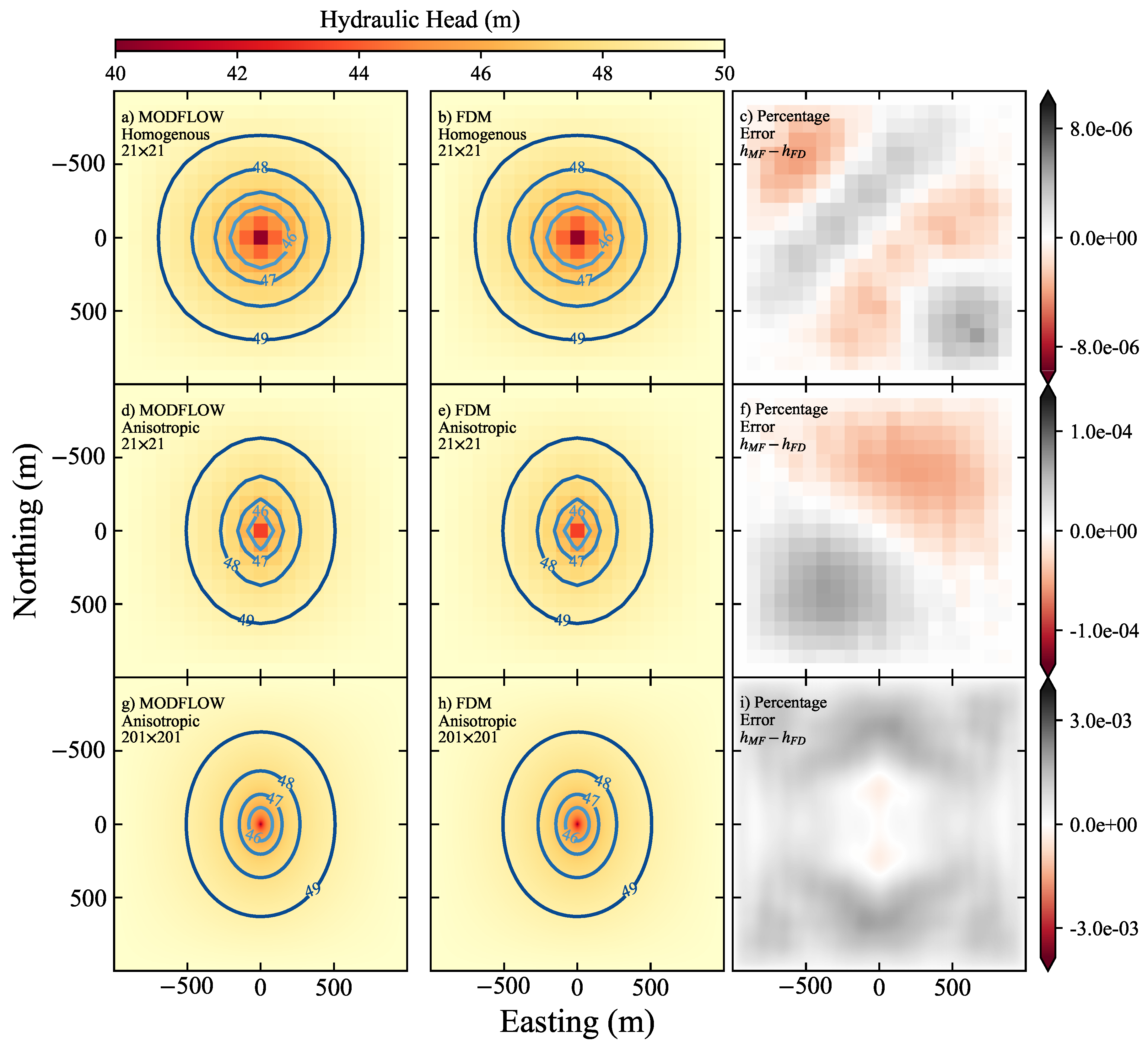
Figure 6.
Vertical and horizontal profile of head results from Figure 5.
Figure 6.
Vertical and horizontal profile of head results from Figure 5.
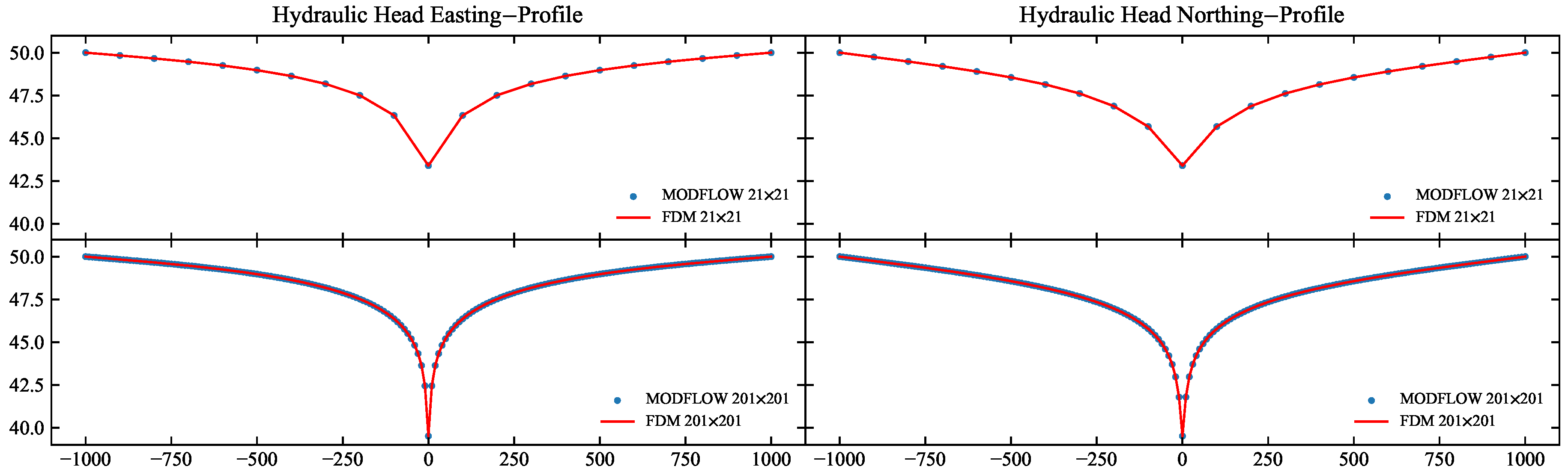
Figure 7.
2D Groundwater simulation for homogeneous media using a) MODFLOW and b) our finite-differences implementation.
Figure 7.
2D Groundwater simulation for homogeneous media using a) MODFLOW and b) our finite-differences implementation.
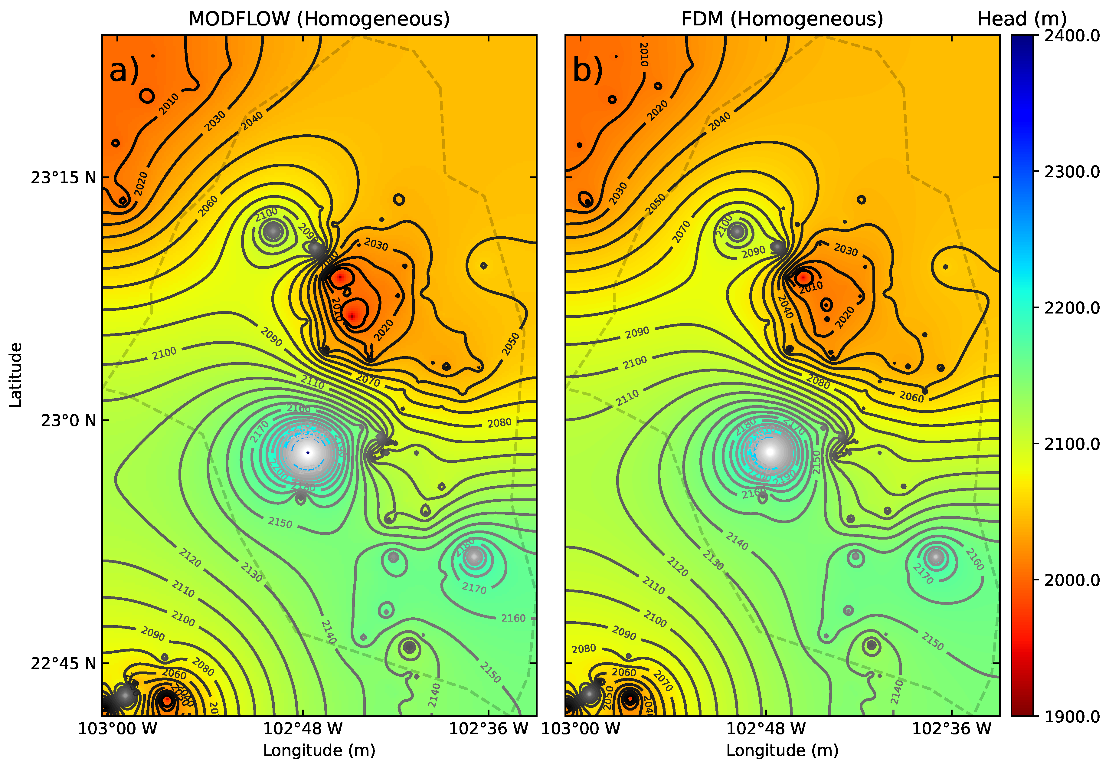
Figure 8.
Exploratory data analysis for the piezometric data.
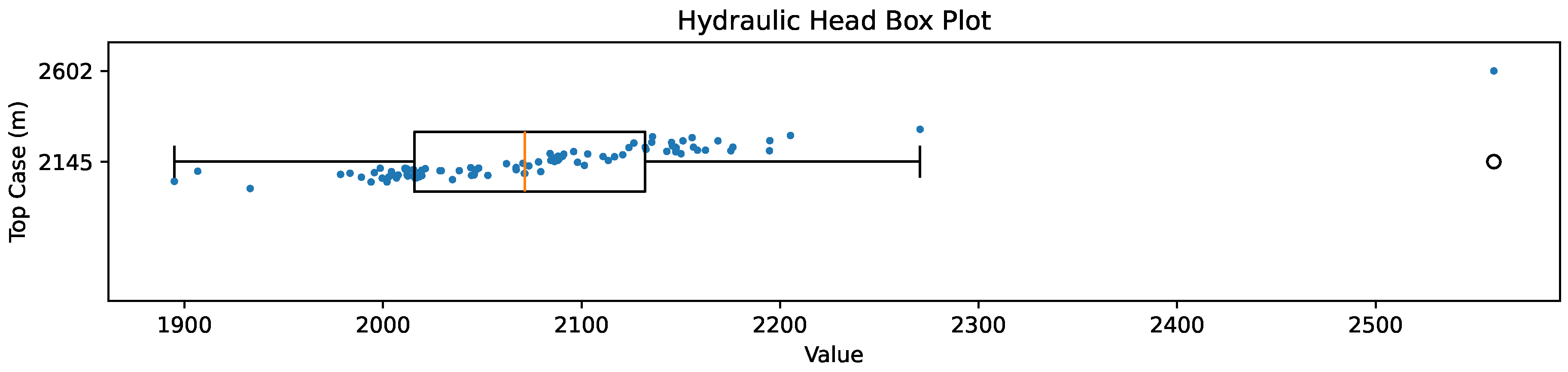
Figure 9.
a) Groundwater modeling on the administrative aquifer of Calera using our FDM implementation for heterogeneous media, and b) Geology and head contours.
Figure 9.
a) Groundwater modeling on the administrative aquifer of Calera using our FDM implementation for heterogeneous media, and b) Geology and head contours.
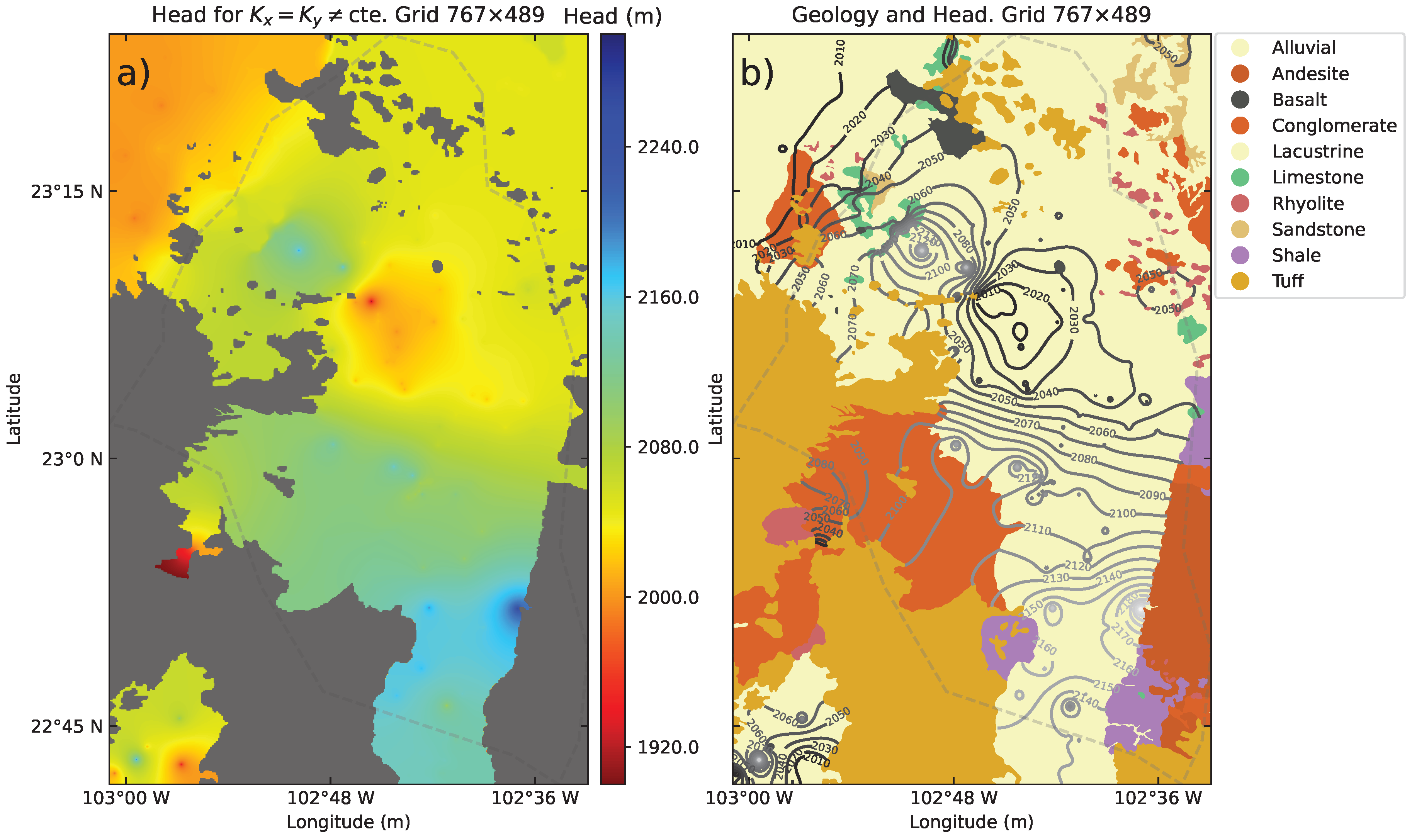

Table 1.
Hydraulic Conductivities for the model construction. Modified from Bear [27]
| Rock | K (m/s) | Rock | K (m/s) |
| Alluvial | Limestone | ||
| Andesite Porfidic | Ryolite | ||
| Basalt | Sandstone | ||
| Conglomerate | Shale | ||
| Lacustrine | Tuff |
Disclaimer/Publisher’s Note: The statements, opinions and data contained in all publications are solely those of the individual author(s) and contributor(s) and not of MDPI and/or the editor(s). MDPI and/or the editor(s) disclaim responsibility for any injury to people or property resulting from any ideas, methods, instructions or products referred to in the content. |
© 2025 by the authors. Licensee MDPI, Basel, Switzerland. This article is an open access article distributed under the terms and conditions of the Creative Commons Attribution (CC BY) license (http://creativecommons.org/licenses/by/4.0/).
Copyright: This open access article is published under a Creative Commons CC BY 4.0 license, which permit the free download, distribution, and reuse, provided that the author and preprint are cited in any reuse.


