
Submitted:
17 November 2025
Posted:
01 December 2025
You are already at the latest version
Abstract
We envision a minimalist way to explain a number of astronomical facts associated with the unsolved missing mass problem by considering a new phenomenological paradigm. In this model no new exotic particles need to be added and the gravity is not modified, it is the perception that we have of a purely Newtonian (or purely Einsteinian) Universe, dubbed Newton-basis or Einstein-basis, actually "viewed through a pinhole", which is "optically" distorted in some manner by a so-called magnifying effect. The κ-model is not a theory but rather an exploratory technique that assumes that the sizes of the astronomical objects (galaxies and galaxy clusters, or fluctuations in the CMB) are not commensurable with respect to our usual standard measurement. To address this problem, we propose a rescaling of the lengths when these are larger than some critical values, say, > 100 pc −1 kpc for the galaxies and ∼1Mpcforthegalaxy clusters. At the scale of the solar system or of a binary star system the κ-effect is unsuspected and undistorted Newtonian metric fully prevails. A key-point of ontological nature rising from the κ-model is the distinction which is made between the distances depending on how they are obtained : a. Distances deduced from luminosity measurements (i.e., the real distances as potentially measured in the Newton-basis, and currently used in the standard cosmological model). b. Even though it is not technically possible to deduce them, the distances which would be deduced by trigonometry. Those "trigonometric" distances are, in our model, altered by the kappa effect, except in the solar environment where they are obviously accurate. In outer galaxies, the determination of distances (by parallax measurement) cannot be carried out and it is difficult to validate or falsify the kappa-model by this method. On the other hand, it is not the same within the Milky Way for which we have valuable trigonometric data (from the Gaia satellite). Interestingly, it turns out that for this particular object there is a strong tension between the results of different works regarding the rotation curve of the Galaxy. At the present time when the dark matter concept seems to be more and more illusive, it is important to explore new ideas, even seemingly very odd, with an open mind. The approach taken here is, however, different from that adopted in previous papers. The analysis is first carried out in a space called Newton-basis with pure Newtonian gravity (the gravity is not modified) and in the absence of dark matter type exotic particles. Then the results (velocity fields) are transported into the leaves of a bundle (observer space) using a universal transformation associated to the average mass density expressed in the Newton-basis. This approach will make it much easier to deal with situations where matter is not distributed centrosymmetrically around a center of maximum density. As examples we can cite the interaction of two galaxies, or the case of the collision between two galaxy clusters in the bullet cluster. These few examples are difficult to treat directly in the bundle, especially we would include time-based monitoring (with evolving κ-effect in the bundle). We will return to these questions later, as well as to the concept of average mass density at a point. The relationship between this density and the coefficient κ, must also be precisely defined.
Keywords:
κ-effect
; anamorphic
; dark matter
; galaxy rotation curve
; galaxy clusters
; bullet cluster
; CMB
; Hoagobject
1. Introduction
Currently the two concurrent most elaborate models which have been built to eliminate the dark matter are:
- -
-
MOND (alternatively seen as a modified inertia or gravity modified theory) of Mordehai Milgrom [9,10]and
- -
- MOG (modified gravity) of John Moffat [11].
Both of these models have known some success in the interpretation of many observational facts at the galactic and galaxy cluster scales. Both have been the subject of numerous publications. Some relativistic versions of MOND also reflect certain aspects of MOG. Nevertheless, any type of modified gravity introduces new particles associated to added scalar and vectorial fields to the Einstein-Hilbert formalism of general Relativity. Then a question comes up : Where are those new particles in the standard model of particle physics ? Introducing new fields in the context of general relativity immediately leads to complete the standard model of the particle physics by quantification. Given the sophistication, the approximations or the ambiguities in the calculations, we must ask ourselves whether such methodology offers a valuable alternative to dark matter. Thus the path of modified gravity could be fraught with unforeseen pitfalls. In any way we believe that modified gravity may one day finally prove to be a false lead in solving the enigma of the missing pseudo-mass. From the outset any modified law of gravity seems to be hardly acceptable for the following simple reason : At millimeter ranges the law of gravity has been tested with a very high accuracy to be the same as between two planets in the solar system (gravitational inverse square law and identical gravitational constant G, cf.for instance [12], although with a huge distance scale factor ). Why should it suddenly be different at the scale of a galaxy (although with a distance scale factor much smaller if we compare the interaction between two stars in a galaxy to that governing the motion of two planets in the solar system)?
Other models have more recently emerged [13–16]. These models spring from altogether different hypotheses, each of them having advantages and disadvantages.
- -
- According to the approach of Verlinde [13], gravity is an emergent phenomenon, starting from a network of qubits which supposedly encode the Universe. Space-time and matter are then treated as a hologram. Dark energy, seen as a property of the network of qubits, interacts with matter to create the illusion of gravity.
- -
- In his approach, Maeder [14,15] wonders whether a part of the difference between the total gravitational mass and the baryonic mass could possibly be explained by exploiting the idea of scale invariance of the empty space.
- -
- A totally different way to eliminate dark matter has been also proposed by Gupta [16]. Unfortunately, the latter model exclusively concerns cosmological items, important questions such as flatness of the galaxy rotation profiles or the mass of galaxy clusters are not considered.
On one hand, up to now all the published models have proposed to change at least one fundamental ingredient in the mainstream physics : inertia, gravity, dynamics, or still to vary the fundamental constants (and even the age of the Universe). On the other hand, we know that, at a "tiny" scale, smaller than a few parsecs (planetary systems, binary stars, stellar black holes or even galactic black holes), the predictions made by the Newtonian dynamics or by general relativity (for high velocities and strong gravitational fields) are verified with incredible precision. Thus, we must check that such exotic remodeling of the well-established laws of physics will not affect our immediate environment (i.e., at the scale of the solar system). By contrast, we show here that the famous ”missing mass conundrum” can also be challenged without loosing any of the well-established principles of the mechanics. Instead of a mechanical origin we rather propose an ”optical” origin [3–8]. In that case the presence of a very huge quantity of (non-baryonic) dark matter could very likely result from an ill-posed problem. This new paradigm (called -effect) appears only when the characteristic dimension of the immense systems studied is much larger than a characteristic length (the domain of galaxies or galaxy clusters ). It is possible that the dimensions of those very huge structures are beyond our direct comprehension, especially if we take for granted at their scale what we know at our small scale. We think that a rescaling of the perceived lengths (and perceived velocities) has to be made. Can we see a kiloparsec as a mere multiple of a meter ? This question is currently posed. This is a kind of relativity which supports some analogy with the Einsteinian relativity where the Lorentz factor () is introduced, expressing how much the measurements of time and length change when the velocity is close to the speed of light. Though the approach assumed in the -model is very elementary, it could eventually and surprisingly solve various astrophysical phenomena. The model is Newtonian, but obtaining a relativistic version is straightforward, it suffices to replace the Newton-basis with a pseudo-Riemannian-basis.
We start from the well-known observational fact that the rotation profile of a spiral galaxy does not match the keplerian profile calculated from the observed density distribution. The observed rotation profile strangely appears as a magnification of the keplerian one. A notable fact is that, following the Sancisi rule, the details of bumps and wiggles are reproduced ([6,17]). Our aim is to reconciliate those profiles thanks to a correspondance principle. We assume a one-to-one correspondance between a domain (called Newton-basis), variable u, where the Newtonian gravity prevails, and a codomain where the observers reside (a leaf of a bundle, variable r). That correspondance should explain the observed non-keplerian profile.
To be more specific, in the Newton-basis a galaxy appears more compact than in the codomain where observers reside, with very tightly winding, quasi-conservative (quasi-solid-body rotation), spiral substructure. By -effect, in the leaves (where the observers reside), the image of this galaxy is distorted by anamorphosis with a strong stretching of the outer regions. The galaxy appears then to have extended untied (and quasi-permanent) arms, antinomically associated to a flat profile for the velocities. This is an example of a phenomenon treated by the -model.
The -effect is not an "optical" illusion as perceived in the classical sense (such as the trivial effect of refraction in any transparent medium), it is rather an effect resulting from some incommensurability between our very tiny instrumentation and the huge size of the galaxies, with the following physical criterion : the larger an object, the lower its average density. Let us eventually note that other proposals as for the dimensionality of very huge systems have been made in the literature [18,19]. In these interesting papers, Varieschi invokes that the dimensionality of galaxies plays a major role, while we suggest a relatively similar idea that it is their size.
The -effect has also some similarities with refracted gravity [20–22] even though in the -model the modification of the gravity is a fictitious procedure. The refracted gravity is a kind of gravitational permittivity of the space, analog to the permittivity known in electromagnetism.
Even though the proposed procedure seems very odd, an idea, as daring as it is, should always deserve careful attention.
This type of new reasoning might offer some help to solve the conundrum of the rotation profiles in the spiral galaxies and also other seemingly very different phenomena.
2. Some Observational Facts
At the present time, a lot of observational facts lead us to conclude that there is a missing mass problem. The four main facts are:
- i.
-
The galaxy rotation profiles :At a large distance from the centre, the rotation profile of a typical spiral galaxy does not decrease as predicted by the newtonian mechanics. The addition of a gigantic spherical halo of dark matter [23], or a modification of the inertia or of the gravity law solves the problem [9–11,24].
- ii.
-
The mass of the galaxy clusters :The mass of galaxy clusters appears generally very high, of an order of about 10 times the visible baryonic mass. Once again, the addition of a halo of dark matter solves the problem, but an adequate modification of the gravity does the job too [25].
- iii.
-
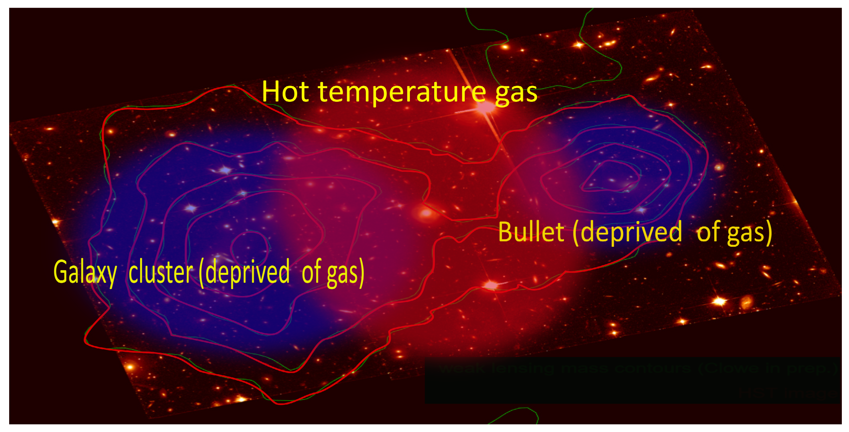
The Bullet cluster :The bullet cluster apparently represents a very rare situation, the lensing diagram is surprinsingly not centered on the baryonic mass (hot temperature gas). The dark matter once again successfully passes the test. By constrast this observation is uneasy to explain in the framework of MOND, whereas MOG manages to do it [26].
- iv.
-
The cosmic microwave background.At the present time : all these observational facts appear definitively understood in the framework of the dark matter paradigm, and not at all by other models, according to the peremptory assertions of dark matter supporters. How is that so certain? Eventually there is the so famous determining test of the cosmic microwave background (CMB) anisotropies. However, it has to be said that both MOG [27] and relativistic MOND [28] easily pass also the latter test.
There exists in facts many models which can explain a wide range of observational facts relative to the missing mass. Dark matter is not the unchallenged leader which is very often described in the literature.
3. Mathematical Background
Let M be a differentiable manifold. A Riemannian metric on M is an application
Where is a definite positive inner product on such that
A -structure on a Riemannian manifold is defined by a smooth function with .
When is a -structure on the manifold
† To each point o of M is associated the Riemannian metric
on M which is a rescaling of the metric g.
† A Riemannian metric on M conformal to g is defined by
Each tangent space is equipped with a set of euclidean norms :
The norms on associated to the different metrics satisfy
Distances :The distances and on M associated to the metrics g and satisfy
and
Connexions :Levi-Civita connexions of and satisfy
and
where and is defined by .
Parallel transport and geodesics :Let be a class curve on M.
A tangent vector field along is an application such that
The g-covariant derivative along is denoted . This operator is defined on class tangent vector fields along by two conditions
† If X is a class tangent vector field defined in a neighborhood of ,
the field along has covariant derivative along satisfying
where is the velocity field of .
† If is a function of class and U a class tangent vector
field along
A tangent vector field U along is g-parallel along when .
For , the parallel transport from to along is the application from to associating to the tangent vector where U is the parallel vector field along such that . It is well-known that is an isometry from to .
A class curve c is a g-geodesic when
It is well-known that when c is a g-geodesic the g-speed, is constant.
As , we have
Let c be a g-geodesics, the g-speed and -speed of c are linked by
The -geodesic are class curves solution to
The -geodesics are a priori altogether different from the g-geodesic curves not even sharing the same supports.
The class curve solutions to
i.e.,
have the same supports than g-geodesics but are parametrized with constant -speed .
-Structure on .
If where is the euclidean metric, for all we have , and are trivial.
In local coordinates, for two tangent vector fields and
:
Let be a class curve and be a class tangent vector field along . If :
A tangent vector field along is parallel when each function is constant.
Let be the parallel transport along from to
Then, when the tangent vector field along is g-parallel, we have
and
The -geodesics and the -geodesics are curves c such as the velocity vector field is parallel along c they are straight lines parametrized with constant velocities , while solutions to
are straight lines parametrized with constant .
4. Applications
Let be a -structure.
- (1)
-
Each trivial cross-sections of the trivial bundleis equipped with the flat Riemannian metrics .For we call o-leaf the trivial cross-section equipped with the metric .
- (2)
- We also get a a priorinon-flat Riemannian metric on
4.1. Postulate of the Kappa-Model
To any point o in the universe we associate a "sitting-observer", O, its phase space is assumed to be euclidean. We assume that the physic locally experienced by a sitting-observer does not depend on its location. For example, two far apart sitting-observers holding hydrogen atom would agree on its size or on its emission spectrum. Therefore an itinerant-standard-meter can be defined using an "apparently" non-deformable object an itinerant-observer would carry while traveling.
 A -effect appears when a sitting-observer uses its local tools of measurement to measure distances between objects located in a region R where the rescaling coefficients is different from its own.
A -effect appears when a sitting-observer uses its local tools of measurement to measure distances between objects located in a region R where the rescaling coefficients is different from its own.4.1.1. Consequences of the Postulate on Metrology
Metrology of distances and consequences
Let E be an earth-based sitting-observer at the location e (the earth).
Let be objects in the Universe, the sitting-observer E interprets the locations of those objects and their possible motions as if they were taking place in the e-leaf, Figure 1.
Technically, there are different ways to estimate distances .
- -
- For close objects (up to about 1 ), the sitting-observer E uses trigonometric parallax methods to estimate radial distances, in other words he uses its local tools and obtains . If and are close enough to e some trigonometry gives the distance i.e the distance in the e-leaf between the "replicas" of and seen by E.
- -
- When an object is located too far away to use parallax methods to evaluate its distance to earth, metric informations are retreived from informations carried by light such as ratios between intrinsic magnitude and observed magnitude (cepheid-method) ; furthermore the number of stars in a given region is not submitted to -effect. In other words the luminosity is not affected by the -effect. Distances measured by those kinds of methods are the distances that an itinerant-observer would get, we denote it and call it photometric distance, they are valid for close galaxies and are distances in the Newton-basis, cfFigure 1. To get an estimate of the distance between two distant objects and , the sitting-observer E has no choice but to use the -effect independant angle and the photometric distances and obtaining that way an "apparent" distance proportional to .
Beside the apparent distance we also have the (non measurable) distances ou 2) in the and -leaves fulfilling the relation
If is a segment located in a region R where the rescaling coefficient is constant we have
Let us now consider and two segments located in two different regions R and where the rescaling coefficients are constant, in R and in . The segments S and have same length in the "Newton-basis" whenever
To any sitting-observer O located at o, S and appear with different lengths :
This induces a distorted perception of the "transverse" shape of distant objects for any sitting-observer as shown in Figure 2 :
Let and be two segments with same length in the Newton-basis located in a galaxy far enought from e so that can be considered as independent of . The ratio of apparent lengths of those segments equals the ratio of rescaling coefficients of the regions containing them. For two regions having same size in the Newton-basis, the region with the lower rescaling coefficient appears wider. As shown in Figure 1, this induces that the shape of obtained by a sitting-observer is anamorphic to its shape in the Newton-basis.
Another effect could be a radial deformation. Assuming that the sitting-observer E measures the radial distances using trigonometric techniques, a region with low rescaling coefficient would appear further away than a region where the rescaling coefficient is higher, even though the photometric distances are the same. Those "trigonometric" distances are fictitious (they are not distances in the Newton-basis) and not measurable because we observe the Universe through a "pinhole" suppressing perspective (such as in the Ames room). To see these effects (if existing) a device of two telescopes separated by more than a few pc would be necessary. Nevertheless this would imply a radial distortion in the leaf of the sitting-observer E. On Figure 3 this distortion is shown in case of a galaxy with decreasing density from its center.
When observing an object with lower density in its central part, like the bullet cluster, the deformation shown in Figure 3 would be reversed : trigonometrically the outer part would appear closer than the central part of such an object.
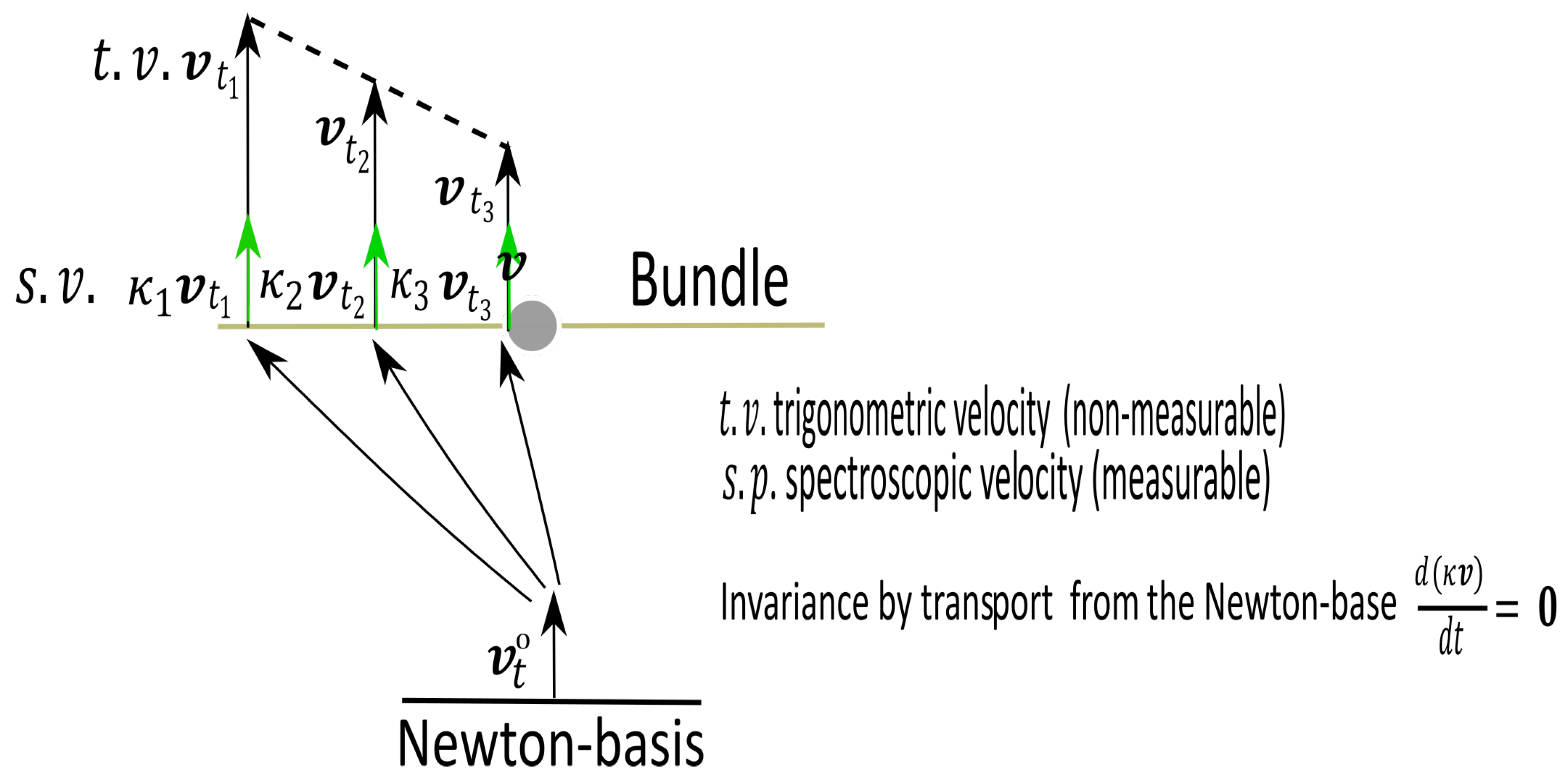
Metrology of velocities
As time is -effect free, frequencies are too, then the spectroscopic measurements of radial velocity, are evaluated as in the Newton-basis.
Transverse velocities are not often technically observable but when and if they were they would be affected by the -effect.
Metrology of masses and densities
We assume that the mass of a given region R of the Universe is unaffected by the -effect. This means that whether a given region is considered in the Newton-basis or in a leaf it has the same mass. On the other hand volumetric mass densities and areal mass densities are, of course, affected by the effect, (with a factor or ).
The -model has no real consequences on what happens on a hidden reality, dubbed Newton-basis. Its consequences are metrologic, not directly perceived at our tiny scale, but yet existing at a very large scale.
According to the -model, measurements of physical quantities which rely in one way or another on the use of a standard meter far away from the observer are affected by the -effect. On the other hand mass, time and luminosity are not submitted to that effect.
As measurement of the areal mass densities are affected by the -effect but spectroscopic velocities are not, the -effect could explain the discrepancy between the keplerian velocity profile predicted by the observed density profile (apparent transverse distances) of spiral galaxies and observed velocity profile (radial velocity), it might also explain the discrepancies as for the evaluation of the dark matter/baryon ratio in the Milky Way, obtained by different methods1. Eventually, the transverse anamorphosis described in Figure 2 might also give an explanation to some anomalous shape observations like the Hoag’s object.
4.1.2. Consequences on the Dynamics
- -
- The usual dynamic equation is changed :
- -
- For a free motion constant we get .
- -
- During a displacement the invariant reference length is . However, a terrestrial observer measures and, if this measurement could be made, he would conclude that the reference length varies in the Universe! (-effect). Obviously this effect is an illusion, the true reference length does not vary (the displacement of an atom does not modify its size).
Some physical quantities are measurable, but others are not.

| measurable | non-measurable |
| Photometric measurement | (fictitious) |
| Spectroscopic velocity measurement | (fictitious) |
| proper motion measurement |
outer region of the galaxy, extragalactic medium.
4.2. Calibration of the Kappa-Effect
We now attempt to reconcile Newtonian mechanics and observations of velocity profiles in the outer rims of spiral galaxies. It happens that the observed velocity profiles do not match the velocity profiles predicted by the apparent distribution of mass. We propose here an adjustment of the -effect so that the velocity distribution and the mass distribution are related in agreement with the effects of Newtonian gravity. The dark matter approach reconciliate observed and predicted velocity profiles by introducing a "missing" mass and consequently modifying the mass distribution, while MOND and MOG approaches modify the Newtonian mechanics. On the other hand the -model approach is different because it modifies the sole perception of geometry, whose consequence is a modification of the mass distribution; but unlike the dark matter model the adjustment of the -effect is directly linked with the observed mass densities.
We request that for objects moving in his immediate vicinity (a few parsecs) a sitting-observer O experiences no discrepancy between predictions of Newtonian gravity and distribution of masses as he measures it, while for far away object (in regions with a rescaling coefficient different from ), the -effect acts and explains the discrepancy between Newtonian predictions and observations.
4.2.1. Mass Distribution and Velocity Profile in a Spiral Galaxy
Mass distribution in a leaf vs mass distribution in the Newton-basis
We assume that to an earth based sitting-observer E a spiral galaxy appears as a flat disk with center C with centrosymmetric apparent mass distribution.
For a point in :
- -
- Let denote the distance in the e-leaf between and the center C of .
- -
- Let be the areal mass density profile apparent to E.
- -
- Let the velocity profile predicted by the Newtonian me-chanics according to the density profile (which is problematically not observed)
A Newton-basis based observer (itinerant-observer) would measure geometric quantities altogether different
With postulate 1 :
- -
- The distance between and C would be
- -
- Assuming conservation of local mass : The mass of a given region does not depend on wether it is measured by a sitting-observer or an itinerant- observer : The areal mass density2 would be
- -
- A velocity profile predicted by the Newtonian mechanics accor- ding to the profile .
Normalizing , we get
Both the function and the distribution are non-observable and therefore unknown, what is observable is the velocity profile associated to the density profile . It should then match, after the anamorphosis , the typical velocity profile observed by E.
Having no direct way of observing neither nor makes it difficult to obtain them.
Looking for a biunivocal pairing reconciliating observed and theoretical velocity profiles would be very interesting because the -model would then rely on a single postulate, without addition of a series of auxiliary (and ad hoc) parameters as it is the case for the dark matter paradigm.
However, for now, a complete adaptation producing a mass distribution in the Newton-basis corresponding to an exponential mass profile observed in the leaves remains an unproven conjecture. We will be working on in the next project, but before some preliminary tests are presented here.
We impose supplementary (reasonable) conditions on the functions and :
- -
- The distribution must be stable to gravitational perturbations.
- -
- The distribution and the rescaling should produce the observed velocity profiles.
It is well-known for a long time that a selfgravitating Newtonian thin disk is very unstable [29]. A compact disk with McLaurin distribution or quite close to it in the Newton-basis could be more stable than the thin and very extended exponential disk which would be fictitiously seen in the leaves, this statement has yet to be checked. Coupled with a rescaling function close to the one already used in our previous works [4–6] the mass distribution should produce velocity profile close to the observed profile.
Another difficulty is that a spiral galaxy is not composed of an unique disk, but of two disks (gas and stars), and also in a number of cases a (small or big) bulge must be added.
When we examine the observed velocity profiles listed in SPARC or other catalogues, we can see that a small series of archetypical profiles appear. Another approach to proceed is to build a catalogue of theoretical cases, assuming a McLaurin-type mass distribution in the Newton-basis. In order to produce a predictive observed velocity profile we do not want to introduce arbitrary parameters (as it is unfortunately the case for dark matter). We impose, nevertheless, some conditions on the couple for each disk.
Condition (C4) springs from the fact that we assume that a point moving radially inward the galaxy should be seen moving radially inward by any sitting-observer.
We required that in the Newton-basis the mass distribution of a spiral galaxy has compact support, following condition C1, the mass distribution of the same galaxy in the sitting-observer leaf must have compact support. This is the reason why we equip the usual exponential distribution (where is the density at the center measured by the sitting observer E) with a strong cut-off at . :
We had here normalized the maximal density : and chose , but this condition is not restrictive and does not alter the generality of our purpose. In other words the quantity is not an arbitrary parameter of the model, we could have choose any value (likewise for the large cut-off exponent 100). We start then with an observed mass distribution profile with support . For sitting-observers located in region with the observed profile are displayed in Figure 4.
The McLaurin-type function has the form given below :
With support and maximal densities where is the rescaling coefficient at the center. The total mass conservation impose a relation between a and A. For instance for we would find . The corresponding density curve is displayed in red in Figure 5.
The McLaurin function has the form given below :
The conservation of the total mass supplies in this case .
Unfortunately, in both cases the function satisfying both Equation (1) and Equation (2) do not fulfill condition C4.
On the contrary, we can choose a rescaling coefficient function fulfilling conditions C1 to C4 and compute the density distribution in the Newton-basis accordingly. The function such that with
satisfies conditions to , we have with and the "-adapted" density distribution in the Newton-basis corresponding to the profile (eq (2)) is
This density profile is displayed in blue in Figure 5.
In Figure 5 we also displayed in dashed red the quadratic mean of the density profile and the McLaurin type profile.
In case of a galaxy modelized by two disks : (stars +gas) the areal mass densities in the Newton-basis and in the leaves are the sum of two areal mass densities with different parameters :
where, for each component ()
and completed with the closure relation
for or the inverse ratio when .
The reference density is the mean density in the vicinity of the Sun (). Another condition which has imperatively to be respected is the invariance of the total masses: for each component.
Velocity profiles in the Newton-basis vs in the leaves
The relation between velocity profiles in the Newton-basis and in the e-leaf is then obtained by using the following relationship, valid for a thin disk
with is the rescaled length r seen in the Newton-basis (we use here the more manageable relation ). The symbols and represent the complete elliptic integrals, respectively of first and second kind.
Figure 6 shows the rotation velocity profiles. We see that the velocity profile corresponding to -adapted profile is a replica of the keplerian curve (following the Sancisi rule and see also [6], where this rule is well checked), but it is now magnified by a factor 1.5-3, while it also appears a little flatter. In order to compare our universal profiles with MOND, We have taken and as reference units for respectively the velocities and the distances (that is 3 for a massive disk with and ).
Whereas a fairly good agreement can be obtained for large distances () between -adapted and MOND profiles, for small distances the -adapted profile presents a hump which is practically absent in the MOND profile. However, while this hump in the keplerian profile is high (peak velocity over terminal velocity of the order of 3), this ratio is lowered to 1.5 in the -adapted profile.
We can see in Figure 5 that the -adapted mass density curve is relatively close to the McLaurin-type one. By contrast in Figure 6 we note that by modifying the density distribution even slightly (of the order of 15 percent) in the Newton-basis, we obtain a very substantial change in the shape for the rotation profile seen in the bundle where any observer has access (of the order of 40 percent for the terminal velocities). Let us also note that the quadratic mean of both -adapted and McLaurin-type (case ) surface density curves would give a quasi-flat rotation profile, with a tiny hump, even though above the MOND profile by (profile displayed in dashed red).
Acceleration profiles
It is also interesting to compare the terminal accelerations from these curves. The results are superimposed to the observational data supplied in [30,31]. The -adapted velocity profile is a close match to a RAR-like (radial acceleration relation) (displayed by a blue line), whereas it is not the case with the McLaurin-type profile (displayed by a red line), which is seen located very far above the observational data (this is due to the fact that the magnification factor for the velocities is too high in the case of a McLaurin-type density profile, of the order of 4, instead of the order of as observed). However this is not a real surprise, because a perfect McLaurin density profile for a disk (taken in the Newton-basis) was already excluded from the outset by the non-fulfillment of the condition C4 and equations (1) and (2) simultaneously.
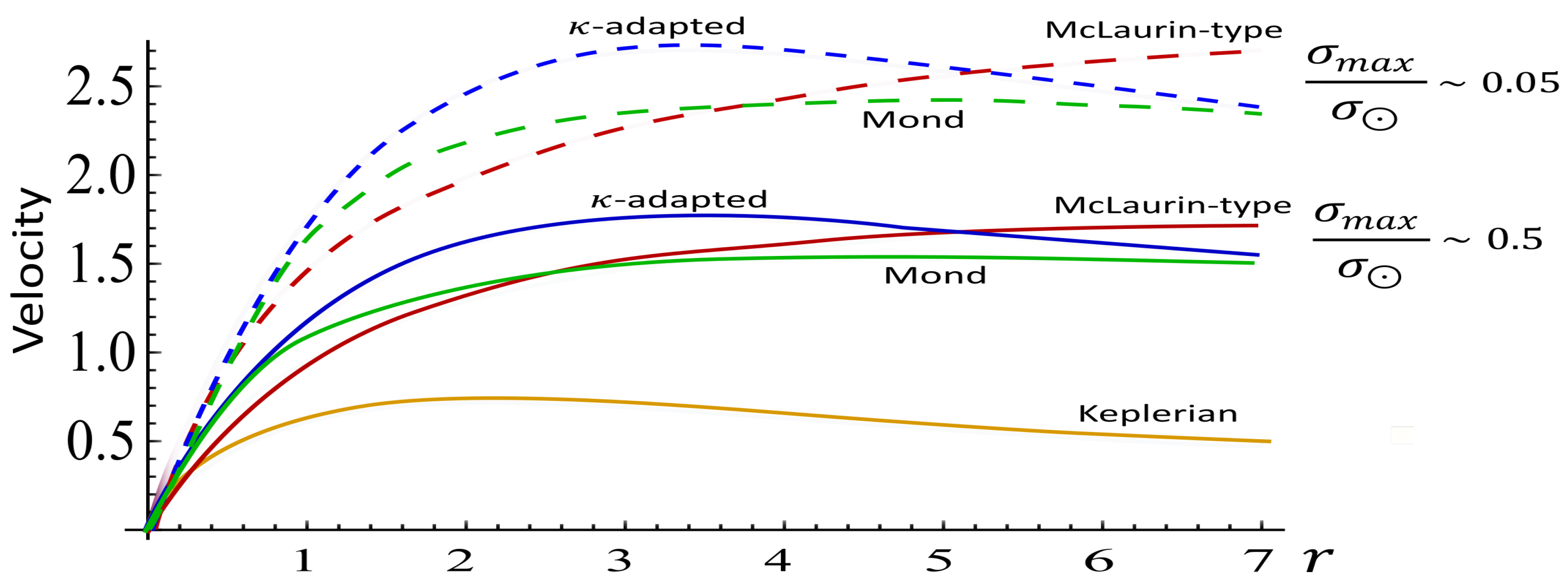
For most of the rotation profiles of the SPARC catalogue [32] corresponding to small galaxies in size (), deprived of a bulge, the keplerian hump (when existing) is smaller than 1.25, we must then limit the universal curves presented in Figure 7, to the range [0, 7]. As references we take now
- i.
- and (for and )
- ii.
- and (for and )
Figure 7.
Radial acceleration relation (RAR). a. reference [30], b. reference [31]. We have surimposed the RAR-like curves of our models (blue: -adapted and red: McLaurin-type)
Figure 7.
Radial acceleration relation (RAR). a. reference [30], b. reference [31]. We have surimposed the RAR-like curves of our models (blue: -adapted and red: McLaurin-type)
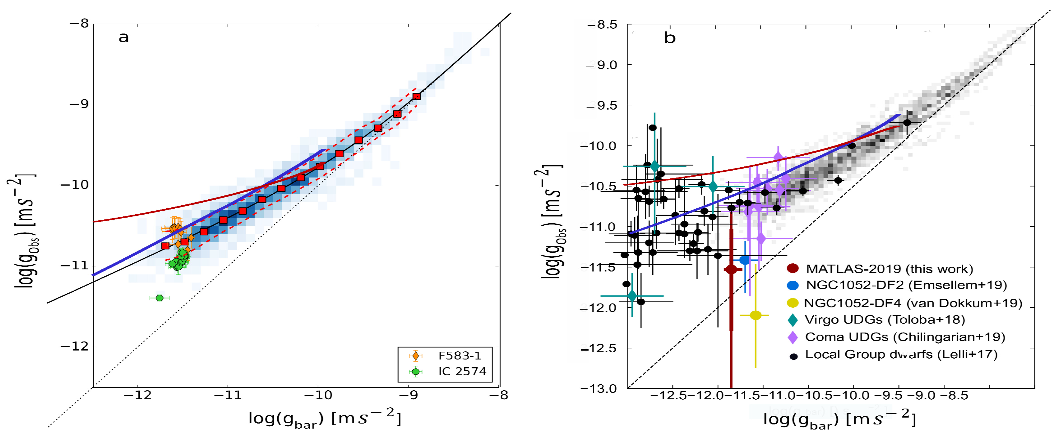
In both of these cases, the magnifcation ratio is high as observed for most of diffuse galaxies, case i. 2.5 (2.0 for MOND) and ii. 3.8 (3.3 for MOND). Such high magnification ratios appear for low accelerations () in MOND and low densities () in the -model. The dark matter paradigm is not able to predict such a statement, apart from an ad hoc manner. In any event, low density (-model) and low accelerations (MOND) seems to be well correlated in the galaxies. The main reason is that the parameter in MOND seems to be itself associated to the mean mass density taken in the Sun vicinity in the Milky Way (solar mean mass density) 4 considered as a density reference for all the densities in -model, let:
MOND and -model give similar profiles for the galaxies [6], especially for the prediction of terminal velocities. However we know that MOND cannot be extended to the galactic clusters without reintroducing some quantity of dark matter, whereas the formalism of the -model can directly be applied to these objects [7].
Another clear difference is however that while in MOND is seen as a cosmological parameter [17], in the -model this paramater is rather seen as a local parameter. In addition we recall that within the dark matter paradigm two or three free parameters by galaxy and an empirical relationship are needed, whereas in MOND just one unique parameter, i.e., , and an empirical relationship are needed. For the -model, there is no longer free parameters, but just an empirical relationship linking the mean density to the scale factor (assuming that in the three models observational measurements lead to the same set of data).
Figure 8.
McLaurin-type, -adapted and MOND velocity profiles for the case i. (continuous lines) and case ii. (dashed lines).
Figure 8.
McLaurin-type, -adapted and MOND velocity profiles for the case i. (continuous lines) and case ii. (dashed lines).
The predicted curves, McLaurin, -adapted and MOND differ between them by . This seems to offer predictions of low quality. Admittedly it is not expected that the observational data are really better (e.g., the Milky Way, M33, etc). However, the agreement between MOND and -model was found yet to be better in [6], but in the latter paper we reasoned directly in the bundle without going through the Newton-basis for which the informations on the mass density profile are still badly known.
Figure 9.
Ratio as a function of . The blue dots are the SPARC data.
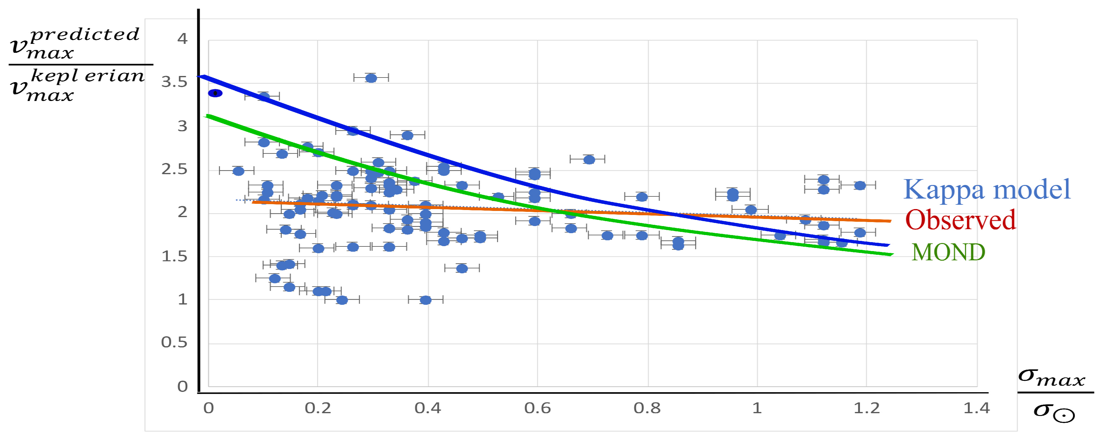
Galaxies with an observed keplerian rotation profile :
Eventually expressing the ratio as a function of shows a fairly good agreement with the observational data from SPARC when . When (ultra-diffuse galaxies) both MOND and -model predict values higher than the observed ratios. Sometimes this ratio is close to the unit (mimicking an absence of dark matter). This represents some tension for MOND or modified gravity; onthe contrary the -model is more flexible and can solve this difficulty by noticing that such low ratios appear for small galaxies with a size smaller than . In this case the geometrical thickness is smaller and the volume density is much higher (for the same surface density), and the ratio is lowered. This statement can even be used as a criterion to predict the geometrical thickness of these galaxies.
4.2.2. Shape of a Spiral Galaxy and Winding Problem.
There are two ways to describe the shape of a spiral galaxy : the shape seen by a (far away) sitting-observer E, (observable) and the shape that would be deduced from measurements made in situin a non observable hidden Newton-basis, in that case the mass distribution is much more concentrated than in the e-leaf (Figure 10, Figure 11).
The winding problem
Another intriguing question is the winding problem of spiral galaxies. In a spiral galaxy the outer matter (stars and gas) lags behind the inner matter causing the spiral substructure to wind up tighter and tighter until ultimately disappearing. The conundrum is solved by various models such as density waves, stochastic self-propagating star formation or still swing amplification theory. However the -model also offers a simple, even though partial, solution [4]. The criterion is based on a measurement of the logarithmic derivative of the angular velocity , let in the Newton-basis and in the bundle , with in the outer region of any galaxy . Figure 12 displays the ratio of these logarithmic derivatives (using the -adapted rotation profile). We can notice that this ratio is smaller than the unity by a factor when , i.e., the spiral substructure can be seen persisting much longer. The winding problem is thus strongly lessened, even though not fully eliminated (the wave density phenomenon has still to be present, but can act now more efficiently). An interesting conclusion is that both flat rotation profile and the almost-steady nature of the spiral design are correlated in the -model. Let us still note that the angular velocity is an invariant of the transform Newton-basis toward bundle. It would seem then that the angular momentum is not conserved in the process, but this fundamental law of the physics is in fact saved when we know that this transport does not represent a "mechanical" reality but is a fictitious transport.
Another approach to the calibration of the κ-effect
The mass invariance when we go from the Newton-basis to the leaves writes
We must solve this differential equation. As an example we take now the archetypical McLaurin function5 (always in the hypothesis of the thin disk)
Let us note again that the numerical factor introduced here and there in the -model (here ) is not an arbitrary (adhoc) parameter. It is automatically determined when we normalize the total mass to the unity (the same as in the bundle by mass conservation). We have also take (for the velocities corresponds to and for the distances corresponds to ). Figure 13a. displays the velocity profile in the Newton-basis and Figure 13b. the corresponding profile in the bundle (what is seen by the terrestrial observer). In the Newton-basis the galaxy possesses a solid-body rotation (and any spiral substructure is conservative), while by contrast in the bundle the velocity profile (measured by spectroscopy) is seen flat beyond 6. Obviously the mass density in the Newton-basis is not a perfect McLaurin profile, also the velocity curve is not perfectly linear. The spiral arms wrap around but the characteristic winding time is now increased by a factor 3-4, i.e., instead of .
Let us note two interesting points. First the ratio (reported from the Newton-basis to the bundle) is of the order of 2. This is the mean ratio observed in the SPARC catalogue (Figure9). The second point is that the velocity curve in the Newton-basis is a linear function of u (as a first approximation, the profile in the Newton-basis is not a perfect McLaurin). Knowing the measured spectroscopic velocity (SPARC catalogue) as a function of the distance r, we can deduce (link between u and r) and then automatically the mean density in the bundle (the inverse of the method used in [6], where the spectroscopic velocities were obtained from the mean density). This work remains to be done.
This illustrates again the deep difference between the trigonometric (not technically measurable, the galaxies appear as frozen images on the sky background) and spectroscopic (real) measurements.
4.3. Other Phenomena Interpreted in the Framework of the Kappa-Effect
The -model was initially built to match galaxy’s rotation profiles without any free parameter. In most cases the mean profiles are represented by monotonous curves, and it is easy to separately fit each of them with two or three parameters, which differ from one case to another, this is the proposal of the dark matter paradigm, therefore its predictive power is weak. This situation is difficult to accept and a lot of authors have tried to conceive models with a minimal number of free parameters. We conceed that the fits obtained with those models are generally not as good as with the dark matter paradigm, but those models remain sufficiently predictive. Today the best model is MOND with just one external parameter. Another criterion is that this model has the same degree of simplicity as the dark matter model. The models of modified gravity recently built by some authors do not always respect this criterion. A contrario, the -model is a phenomenological model, the cause of the apparent magnification of lengths is not explicited and remains undetermined, but this magnification is fictitious and depends on the observer.
The -model produces rotation profiles for spiral galaxies substantially similar to MOND [6] (Figure 14). Other differences exist with dark matter. It is difficult to conclude at this stage, because dark matter follows an ad hoc path which in any situations runs, even if the observed curve is biased (such as a bad inclination or distance). For instance for M33 (Figure 14) a clear break in the profile appears at , likely because the inclination suddenly changes. This effect is not taken into account by the theoretical curves. In this case what is the best profile ? Yet by contrast to dark matter, MOND, MOG and -model supply predictive, even though imperfect, methods. A larger sample of galaxies is presented in [6].
Surprisingly enough the -model applies also to a rather heterogeneous set of phenomena seemingly not connected. Indeed, at the present time, these phenomena have been explored following very different theoretical ways:
4.3.1. The Mass of the Galaxy Clusters
The -model has been also applied to the missing mass of galaxy clusters. Once again it succeeds to predict the apparent newtonian mass, and can rivalize with MOG [25] (Figure 15), but without the need to modify the gravity. A larger sample of galaxy clusters is presented in [7].
4.3.2. The Bullet Cluster
The bullet cluster illustrates an unusual aspect of the -model, the possibility to have superimposed images when a region with a weak density is surrounded by a region with a much higher density [7]. The effect is fictitious, but the "reality" for us is what we observe (i.e., the images received on our telescopes). On Figure 16 the dark matter and kappa-model diagrams are compared and appear rather similar, even though the interpretations provided are very different. Figure 17 displays the gravitational lensing diagram observed for the Bullet cluster.
a It is much simpler to make the -model relativistic than in the case of the MOND model. Replacing the Newton-basis with the Einstein-basis is enough. We start from the (fictitious) associated to the proper leaf of the terrestrial observer
- We apply the -transform (or corresponding principle) on this quadratic form
- (the time is left unchanged by the -transform), ().
- and
- , ).
- and do not reside in the same space ( is in the tangent space), and are independant. Thus, more generally, they can even be multiplied by a different factor. Then we obtain the true , that is to say the one expressed in the Einstein-basis
Figure 17.
Gravitational lensing diagram observed for the Bullet cluster [41,42]
4.3.3. The Anisotropies of the Cosmic Background (CMB)
Up to now the application of the -model to the anisotropies of the cosmic background has not been made. The Newtonian theory of Small Fluctuations presented by Moffat and Toth [27] is easily transposable to the -model. Manipulating three fundamental equations (the continuity equation, the Euler equation and the Poisson equation), these authors obtain the equation for every Fourier mode of the fractional amplitude of the density perturbation (in [27] eq. 34 (Newtonian gravity) and eq. 64 (modified gravity) are similar)
where H is the Hubble constant, the speed of sound and the co-moving wavenumber, the constant G is the gravitational constant, i.e., in Newtonian gravity, but G becomes variable in modified gravity MOG (in this case the notation is ). In this equation the modification made by the kappa-model affects , the density. Let be the measurement of volumic density made by a terrestrial observer, and the volumic density that would be measured locally, in other words in the Newton-basis. The relationship between the two is given by the exponent 3 expresses the dimensionality change (2 (spiral galaxy) (one imprinted spot in the CMB)). We find . Let us note that with . The substitution of by mimicks a change of the value of G (in the sense of ) as in MOG : . Let us remark however, that the magnified value of the gravitational constant is fictitious in the -model, whereas this magnification is real in MOG. At this stage we have not performed the detailed calculation of the angular power spectrum of the CMB. This work remains to be done, but very likely we should arrive to the same conclusion as in the paper of Moffat and Toth, the kappa-model should be able to reproduce the CMB acoustic power spectrum.
4.3.4. The Hoag’s Object
The Hoag object morphology can be explained in the sole context of the -model. A lot of various and interesting scenarios have also been provided by other authors [43–46]. Thus Bannikova [45] explains very clearly why the hole does not fill up, because the trajectory of any particle located in it is definitely unstable. However, how did Hoag’s object form and when? The usual scenario for describing ring formation relies on the action of a central bar on a spiral substructure. Unfortunately, as for this otherwise interesting scenario, what is enigmatic here is that the bulge appears perfectly circular. The -model can supply a solution: The Hoag’s object is a distorted image of a common spiral galaxy, but characterized by an unusal very strong gradient of density between a very dense bulge and a very thin disk.
Hypotheses :
The Hoag’s object is assumed here to be centrosymmetric. From the center the radial coordinate is denoted u in the Newton-basis and in the e-leaf. At a point the density in the Newton-basis is denoted while apparent density in the E-leaf is denoted .
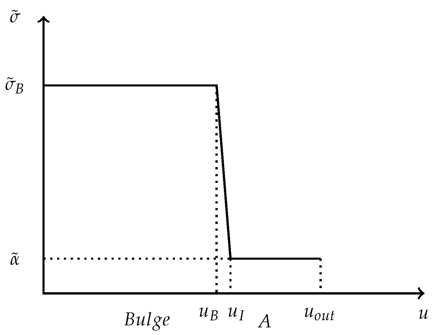
The Hoag’s object appears divided in three regions (Figure 18):
1. A bulge B with a constant projected apparent mass density along the line of view , constant rescaling coefficient and apparent radius . According to postulate 1 radii of the bulge in the e-leaf and in the Newton-basis are linked by , its density in the Newton-basis is constant and .
2. A bulge-disk transition annulus T very narrow when seen in the Newton-basis extending from radii to with (), with density decreasing from ( in the e-leaf) to ( in the E-leaf).
3. An annulus A with constant projected apparent mass density along the line of view , constant rescaling coefficient , extending from apparent radii to when we normalize .
Figure 18.
Schematic density profile for the Hoag object as seen in the Newton-basis.
According to postulate 1, for points in the bulge we have , for points we have this gives :
Concluding remarks :
The condition over expresses a very steep front for the density, what is difficult to obtain, hence the extreme rarity of the Hoag’s object. The left image in Figure 19 displays the appearance of the Hoag object in the Newton-basis. We can see it as a spiral galaxy with a very big bulge surrounded by a narrow disk (type SAa of the de Vaucouleurs classification).
We have tried to apply the -model to the Hoag object for which no process of formation has been clearly identified. A first explanation has been proposed by Hoag himself [47], who suggested that the phenomenon was due to a gravitational lensing. Unfortunately, in that case, the radial velocities of both the bulge and the ring would be very different, whereas the observations show the contrary. On the other hand the -effect is a kind of lensing, but in which the radial velocities are left unchanged, in this case velocities are the same for the bulge and the ring, in agreement with the observations, the luminosity distance being also the same for the two objects. The -lensing differs from the gravitational lensing that bends the trajectory of light rays, the -lensing appears when we try to relate an immense length (the size of a galaxy) to a standard length adapted to our very modest scale.
- A possibility for two superimposed images of a same galaxy
The -model predicts the existence of an unique photometric image. Perhaps, a much more complete version of this model could support the intriguing possibility, in some exceptional circumstances, to have two photometric images of the same galaxy. This suggestion is at this stage, entirely speculative7. Before we investigate further, and even if this statement seems very unlikely, it would be very interesting to measure the radial velocity of the second, with very low luminosity, annular galaxy seen inside the gap region of the Hoag object.
4.4. MOND Versus MOG Versus Kappa-Model
Each of the three models MOND, MOG and -model aim to understand the dynamics of galaxies and galaxy clusters, even though deep differences are existing. A key feature of MOND is that it is a theory governed by an unique fixed acceleration scale, named . A model with a few number of parameters is better than one with a large number, but this can also be a weakness. Thus MOND is facing difficulties when the scale of objects is drastically changed (galaxy clusters). By comparison MOG is more flexible. In MOG gravity is stronger than it would be in general relativity. However, this excess of gravity is canceled out in part by a repulsive force due to a vector field interaction of finite range. This cancellation is produced in the inner regions of galaxies where the behavior is given by the general relativity. At a great distance from the center, galaxies rotate faster because the repulsion vector is absent there, so gravity becomes stronger. The coupling and mass parameters governing the range of the vector force are scalar fields which values vary from system to system. MOG is governed by a hierarchy of scales which is determined by the mass and distance from the source. Unfortunately the counterpart is that MOG introduces extrafields and new particles (not predicted by the standard model of particle physics). Another characteristic of MOG is the variation of the gravitational constant G. This coud be a big problem, because changing G necessarily implies a change for the other physical constants (such as the speed of light). What then are the consequences for MOG ? Very sensitive laboratory tests and observations at the scale of the solar system have not shown any clear deviations from general relativity that would support MOND or MOG (even though this in no way invalidates them). More especially MOND predicts that the dynamics of a system deviates from Newtonian smaller than . This deviation ought to be detectable in wide binaries [48]. By contrast to MOND, both MOG and -model (tiny system regime) predict that the gravitational dynamics of wide binary star systems follows Newton’s law. Various investigations have been performed relative to this important issue [48,49], but the conclusion is still pending.
5. Conclusion
The -model is supported by an alternative line of investigation designed to solve a lot of astrophysical problems which, so far, have not received, according to us, satisfying explanations. The great interest of this model is that the physics of gravity, very accurately proved at the scale of the solar system, is left unchanged (following the Newtonian or Einsteinian version according to the chosen basis). The distances calculated by luminosity measurement (following the usual methods) and the velocities resulting from spectroscopy are left inchanged. In constrast the angular measurements and trigonometric distances (the latter ones being not accessible today) are both strongly affected by the -effect. This effect produces a magnification of all astrophysical objects, taken individually and projected on the sky plane : spiral galaxies, galaxy clusters, spots of the CMB, etc. The -effect acts as a kind of invisible giant lens distorting the Universe seemingly in a anamorphic manner. Is there a hidden reality where the usual physics fully prevails (pure Newtonian mechanics or general Relativity), with no dark matter, and to which we would only have visual access through a distorted (stretched) copy ? The question is asked in this paper.
The recent discovery that the flat weak lensing profile for spiral galaxies appears to continue over very large distances [33,34] also warrants examination within the framework of the -model. Analysis of this issue is progressing, and its importance lies in its potential to differentiate between the -model and MOND theory.
Finally, it should be noted that the -model retains dark energy, a necessary ingredient to explain the acceleration of the Universe. The concept of dark energy is much more credible than that of dark matter, because dark energy can be linked to vacuum energy, which has been proven to exist both theoretically and in the laboratory at the atomic scale (even if there is a serious quantitative disagreement between the two).
Appendix A. Trigonometric Distances and κ-Curvature
Let and be two regions on which the rescaling coefficients are constant, in and in . Let A and B be two sitting-observers respectivelly in the -leaf and the -leaf. We assume that and are small enough and far apart enough so that for a in and b in we can consider that the luminosity distances is constant. Let be in and be in such that , ℓ can be seen as a distance unit common to A and B. We have and . In the small angle approximation, if two photons start from b and and converge toward A, the angle measured by A is whereas the angle between the trajectories of the two photons measured by B is , , the angle is the -aberration angle. If the sitting-observers B and A use now those angles and the common unit distance to measure distance , the results are found to be different.
The distance is seen asymmetrically by the two sitting-observers.
If between the two regions the environment is characterizes by a constant value of the rescaling coefficient , (the situation we have in mind is of two regions in two distant galaxies separated by an homogenoous extragalactic medium) sitting-observers measures
The motion of a particle in the bundle has two components : one component in the basis space and one virtual component in (where and are the minimal and maximal values of on ), the latter component depends directly on the function and the component in the basis space.
Consider two particles whose motions are rectilinear when projected on (solid lines), starting parallel from the observer B the particles arrive parallel at the observer A (but nobody can see the real trajectories in the totality!). Yet for the observer A, the projected trajectories (dashed lines) on his proper sheet (constant ) appear curved along some portions of the trajectories (Figure A1.a). This fictitious curvature is due to the fact that the particle passes from leaf to leaf during its motion in the bundle.
A simpler way to describe this would be to consider an itinerant-observer I traveling from earth, E, to distant points D and in carrying a bag full of standard meters. Once arrived he leaves one of them at D and another at D’ then comes back home to earth. I has two ways of measuring the distance between E and . Counting how many standard meters he had traveled to get the luminosity-distance or, once back home, by trigonometry using the solid angle subtended by the standard meters he had left at D and , he gets the trigonometric distance . The ratio can be seen as a "curvature".
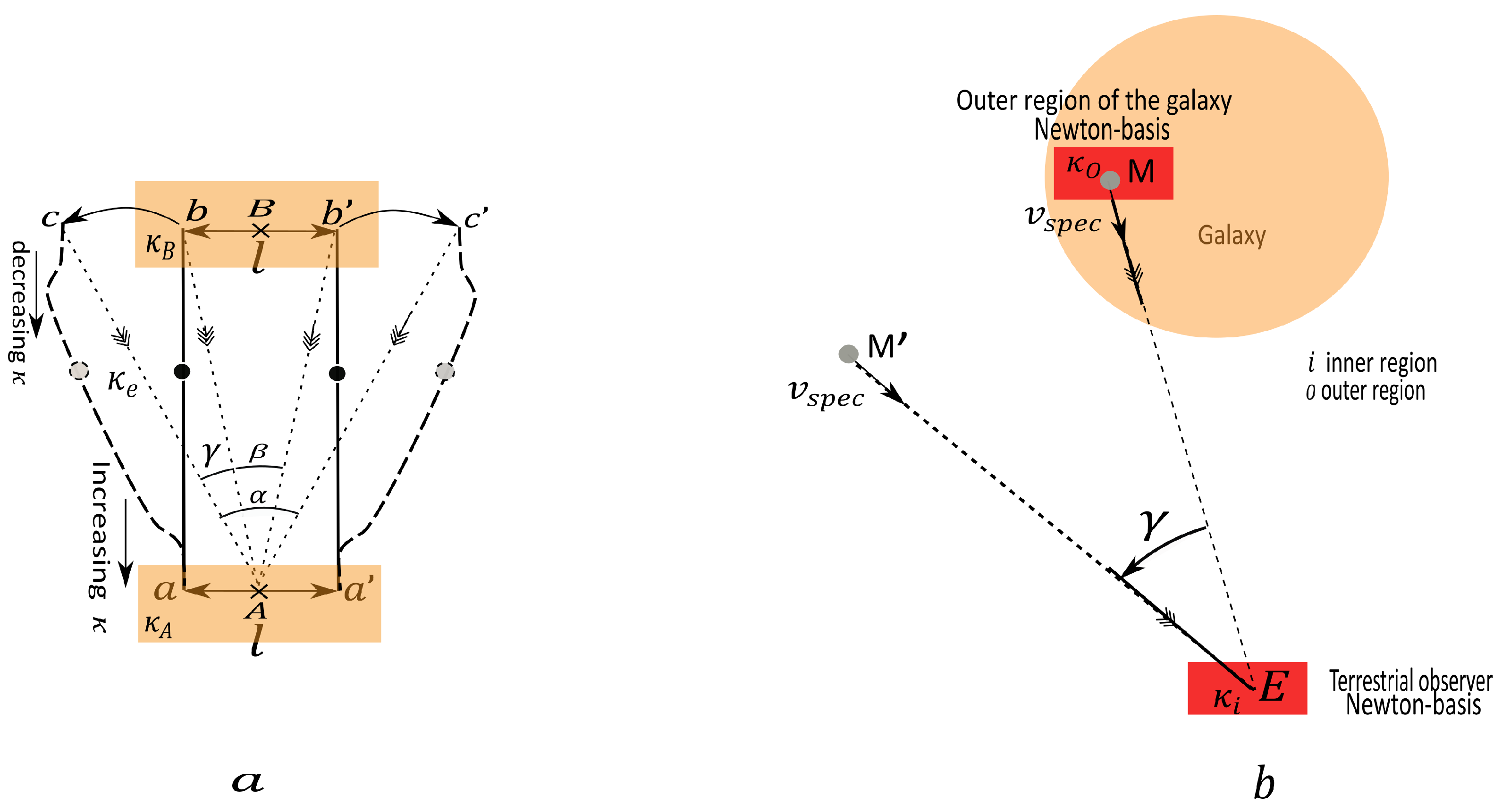
In Figure A1.b we have represented two pieces of the Newton-basis. However these pieces (rather here their counterparts reported in the bundle) are not located in the same sheet of the bundle. The trajectory of the photon appears to be discontinous to any sitting-observer. A great interest would be to know the physical origin of this phenomenon (see appendix B). Two explanations can be suggested: the incommensurability of cosmical distances when compared to those at our tiny scale, or a new and unknown property of light when propagating over a very large distance. When admitted we can see that the kappa-effect acts as a kind of giant lens for the terrestrial observer. The real point M located in the outskirts of a galaxy is seen displaced at the virtual position (Figure A1.b). The size of the observed galaxy (disk) is magnified, whereas the spectroscopic velocity being not affected by the -effect is transported from M to without change.
Figure A1.
Trajectories of photons.
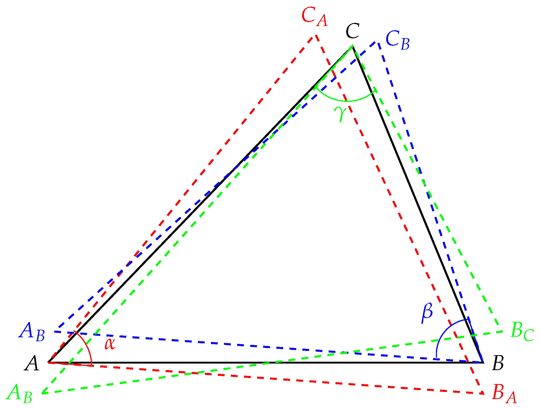
Let us consider three sitting-observer and C in regions with different rescaling coefficients (Fig A2). In each leaf, photons propagates along straight lines. B and C emit photon in direction of A, the angle between the reception direction at A is , but in its leaf A sees B at and C at . By permutation of and C, we can define in the same way the angles of reception (resp ) at B and C. The angles and are the angles at and C of the triangles and , we have which can be interpreted as the existence of a curvature.
Figure A2.
Triangle in the basis and in the leaves.
Appendix B. The Origin of the κ-Aberration
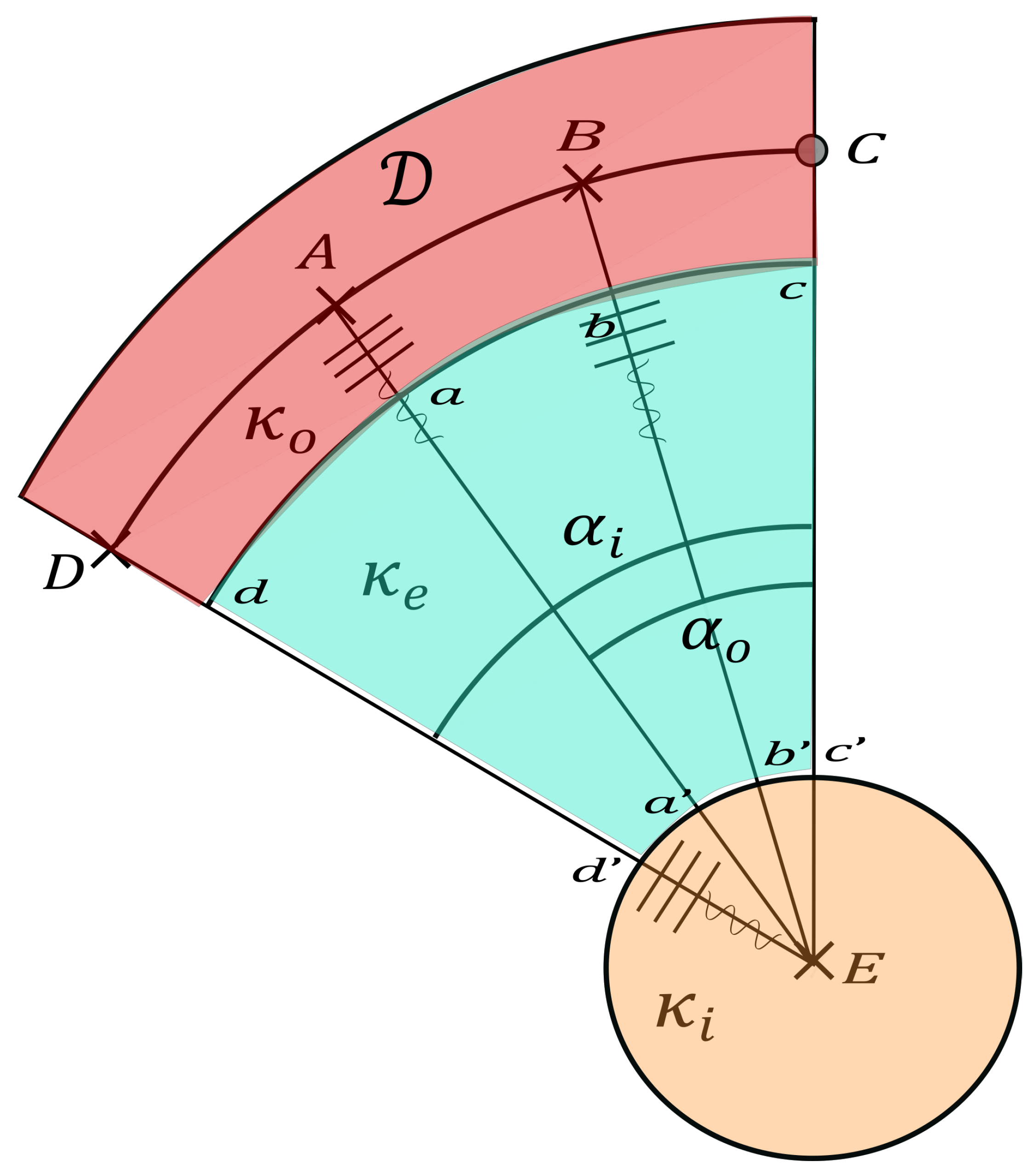
The -aberration is intriguing, because it seems to underline a real change in the direction of the emitted photon, whereas paradoxically enough, the light propagates in straight line in the Newton-basis. This statement is not amenable to easy visualisation, when the dimensions of the objects are very huge. This is the same thing at the atomic scale, in the quantum world the objects are no longer directly visualisable. Let a domain representing a piece of a spiral galaxy (center C) (Figure A3). The linear dimension of is assumed to be very small with respect to the distance ( a few arc-min). This region is separated from the terrestrial observer (coefficient ) by a very extended extragalactic domain (coefficient ). The emitter is located at A in the outer region of the galaxy (coefficient , with the hierarchy ). This emitter is seen at B by any sitting-observer located in the intermediary extragalactic region, and situated at D by the earth-based sitting-observer E. Yet in reality the points and D coincide in the Newton-basis, While these points (or rather their replicas) appear separated in the bundle. Inversing the travel of a photon emitted by A and reaching E is more interesting. If E emits a photon (in the form of a spherical wave) toward the observed galaxy, the photon will be received at A (real), B (fictitious) and D (fictitious but appearing real for E) simultaneously (the distances , and are assumed to be equal); but any way A, B, and D corresponds to an unique point in the Newton-basis.
An analogy with the refraction phenomenon in a medium of variable index can be made. With help of Figure A3, we have
and with the Thales theorem
we obtain a revisited Snell law
the ratio playing the role of a refraction index. However the analogy must not be taken at face value because there is no light-refracting medium.
Figure A3.
-aberration.
Appendix C. The Translation of an Extended Object (Galaxy) Within the Framework of the Kappa-Model
Eventually the analysis of the global motion of a system (a galaxy or an individual galaxy cluster) is interesting. An essential point is that if we can measure the trigonometric velocities, we would have the impression of seeing the galaxy distort with time. This effect is obviously fictitious in the kappa-model; only the spectroscopic velocities represent a reality (a local observer, assumed to be present in the observed galaxy at a given instant, and to be at rest with respect to the terrestrial observer, would measure the same spectroscopic velocity).
Figure A4.
Translational motion of a galaxy seen pole-on. A terrestrial observer is associated to a piece of the Newton-basis
Figure A4.
Translational motion of a galaxy seen pole-on. A terrestrial observer is associated to a piece of the Newton-basis
References
- Beordo, W., Crosta, M. and Lattanzi, M.G. Exploring Milky Way rotation curves with Gaia DR3: a comparison between ΛCDM, MOND, and general relativistic approaches. JCAP 2024, 12, 024. [CrossRef]
- Jiao, O., Hammer, F., Wang, H., Wang, J., Amram, P., Chemin, L. and Yang, Y. Detection of the Keplerian Decline in the Milky Way Rotation Curve. A&A 2023, 678, A208. [CrossRef]
- Pascoli, G.; Pernas, L. Some Considerations about a Potential Application of the Abstract Concept of Asymmetric Distance in the Field of Astrophysics. 2020. Available online: https://hal.science/hal-02530737.
- Pascoli, G. The κ-model, a minimal model alternative to dark matter: Application to the galactic rotation problem. Astrophys. Space Sci. 2022, 367, 62. [CrossRef]
- Pascoli, G. arXiv: 2205.03062 2022b. [CrossRef]
- Pascoli, G. The κ-Model under the Test of the SPARC Database. Universe 2024, 10, 151. [CrossRef]
- Pascoli, G. A comparative study of MOND and MOG theories versus the κ-model: An application to galaxy clusters. Can. J. Phys. 2023, 101, 11. [CrossRef]
- Pascoli, G., Pernas L. Is Dark Matter a Misinterpretation of a Perspective Effect? Symmetry 2024,16, 7, 937. [CrossRef]
- Milgrom, M. A modification of the newtonian dynamics : implications for galaxy systems. ApJ. 1983, 270, 384. [CrossRef]
- Milgrom, M. MOND theory. Can. J. Phys. 2015, 93, 107. [CrossRef]
- Moffat, J. Scalar–tensor–vector gravity theory. JCAP 2006, 03, 004. [CrossRef]
- Yang, S-Q., Zhan, BG., Wang, QL., Shao, CG., Tu, LC., Tan, WH., and Luo. J. Test of the Gravitational Inverse Square Law at Millimeter Ranges. Phys.Rev.Lett.2012, 108, 081101. [CrossRef]
- Verlinde, E.P. Emergent Gravity and the Dark Universe SciPost Phys. 2017, 2, 016. [CrossRef]
- Maeder A. Dynamical Effects of the Scale Invariance of the Empty Space: The Fall of Dark Matter? Apj 2017, 849, 158. [CrossRef]
- Gueorguiev, V.G. and Maeder, A. The Scale-Invariant Vacuum Paradigm: Main Results and Current Progress Review. Symmetry 2024, 16, 657. [CrossRef]
- Gupta, R. Testing CCC+TL Cosmology with Observed Baryon Acoustic Oscillation Features. ApJ 2024, 964, 55. [CrossRef]
- Famey, B., and McGaugh, SS. Modified Newtonian Dynamics (MOND): Observational Phenomenology and Relativistic Extensions. Living Astronomy 2012, 15, 10. [CrossRef]
- Varieschi, G.U. Relativistic Fractional-Dimension Gravity. Universe 2021, 7, 387. [CrossRef]
- Varieschi, G.U. Newtonian fractional-dimension gravity and the external field effect. Eur. Phys. J. Plus 2022, 137, 1217. [CrossRef]
- Cesare, V., Diaferio, A., Matsakos, T., Angus G. Dynamics of DiskMass Survey galaxies in refracted gravity. A&A 2020, 637, A70. [CrossRef]
- Cesare, V., Diaferio, A., Matsakos, T. The dynamics of three nearby E0 galaxies in refracted gravity. A&A 2022, 657, A133. [CrossRef]
- Cesare, V. Dark Coincidences: Small-Scale Solutions with Refracted Gravity and MOND. Universe 2023, 9(1), 56. [CrossRef]
- Li P. The Dark Matter Problem in Rotationally Supported Galaxies. Thesis, Case Reserve Western University 2020.
- Moffat J.W., Rahvar S. The MOG weak field approximation and observational test of galaxy rotation curves. Mon Not. R. Astron. Soc. 2013, 436, 1439. [CrossRef]
- Browstein J.R., Moffat J.W. Galaxy cluster masses without non-baryonic dark matter. MNRAS 2006, 367, 527. [CrossRef]
- Browstein J.R., Moffat J.W. The Bullet Cluster 1E0657-558 evidence shows modified gravity in the absence of dark matter. MNRAS 2007, 382, 29. [CrossRef]
- Moffat J.W., Toth V.T. Cosmological Observations in a Modified Theory of Gravity (MOG). Galaxies 2013, 1, 65. [CrossRef]
- Skordis C., Zlosnik T. New Relativistic Theory for Modified Newtonian Dynamics. Phys. Rev. Lett. 2021, 127, 161302. [CrossRef]
- Ostriker J.P., Peebles P.J.E. A Numerical Study of the Stability of Flattened Galaxies: or, can Cold Galaxies Survive?. ApJ 1973, 186, 467. [CrossRef]
- Lelli F., McGaugh S.S., Schombert J.M. and Pawlowski M.S. One Law to Rule Them All: The Radial Acceleration Relation of Galaxies. ApJ. 2017, 836, 152. [CrossRef]
- Mülller, O. et al. Spectroscopic study of MATLAS-2019 with MUSE: An ultra-diffuse galaxy with an excess of old globular clusters. A&A 2020, 640, A 106. [CrossRef]
- Lelli, F., McGaugh, SS., Schombert, J. M. VizieR Online Data Catalog: Mass models for 175 disk galaxies with SPARC. AJ 2016, 152, 157L. [CrossRef]
- Mistele, T., McGaugh, SS., Lelli, F., Schombert, J.M., and Li P. Indefinitely Flat Circular Velocities and the Baryonic Tully-Fisher Relation from Weak Lensing. ApJL 2024, 969, L3. [CrossRef]
- Chan M.H., Zhang Y., Del Popolo A. Are the Galaxies with Indefinitely Flat Circular Velocities Located Inside Large Dark Matter Haloes? Universe 2025, 11, 4. [CrossRef]
- Corbelli E. and Salucci P. Testing modified Newtonian dynamics with Local Group spiral galaxies. MNRAS 2007, 374, 1051. [CrossRef]
- Banik I., Thies I., Famaey B., Candlish G., Kroupa P. and Ibata R. The Global Stability of M33 in MOND. ApJ 2020, 905, 135. [CrossRef]
- Corbelli E., Thilker D., Zibetti S., Giovanardi C., and P. Salucci. Dynamical signatures of a ΛCDM-halo and the distribution of the baryons in M33. A&A 2014, 572, A23. [CrossRef]
- Kam S.Z., C. Carignan, Chemin L., Foster T., Elson E. and Jarrett T.H. H i Kinematics and Mass Distribution of Messier 33. AJ 2017, 154,41. [CrossRef]
- Reiprich; T.H, Cosmological Implications and Physical Properties of an X-Ray Flux-Limited Sample of Galaxy Clusters. Ph.D.Dissertation, Ludwig-Maximilians-Universität, München 2001.
- Reiprich, T.H., Böhringer, H. The Mass Function of an X-Ray Flux-limited Sample of Galaxy Clusters. ApJ 2002, 567, 716. [CrossRef]
- Bradač, M., Schneider, P., Lombardi, M., Erben, T. Strong and weak lensing united. I. The combined strong and weak lensing cluster mass reconstruction method. A&A 2005, 437, 39. [CrossRef]
- Bradač, M., Clowe, D., Gonzalez, A.H., Marshall, P., Forman, W., Jones, C., Markevitch, M., Randall, S., Schrabback, T. and Zaritsky, D. Strong and Weak Lensing United. III. Measuring the Mass Distribution of the Merging Galaxy Cluster 1ES 0657–558. ApJ 2006, 652, 937. [CrossRef]
- Finkelman, I., Moiseev, A., Brosch, N., Katkov, I. Hoag’s Object: evidence for cold accretion on to an elliptical galaxy. MNRAS 2011, 418, 1834. [CrossRef]
- Brosch, N. Finkelman, I., Tom Oosterloo, T., Gyula Jozsa, G.,and Alexei Moiseev. HI in HO: Hoag’s object revisited. MNRAS 2013, 435, 475. [CrossRef]
- Bannikova, E.Y. The structure and stability of orbits in Hoag-like ring systems. MNRAS 2018, 476, 3269. [CrossRef]
- Hoag, A. A peculiar object in Serpens. AJ 1950, 55, 170. [CrossRef]
- Hernandez, X., Cookson, S. Cortés, R.A.M. Internal kinematics of Gaia eDR3 wide binaries. MNRAS 2022, 509, 2304. [CrossRef]
- Chae, K.H. Breakdown of the Newton–Einstein Standard Gravity at Low Acceleration in Internal Dynamics of Wide Binary Stars. Astrophys. L. 2023, 952, 128. [CrossRef]
- Banik, I., Pittordis, C., Sutherland, W., Famaey, B., Ibata, R., Mieske, S. Zhao, HS. Strong constraints on the gravitational law from Gaia DR3 wide binaries. MNRAS 2024, 527, 3, 4573. [CrossRef]
| 1 | As a matter of fact the estimate of the content in dark matter strongly varies following the method used [1, 2]. On the contrary, in the -model the proper motions (tangential motions) and the radial motions estimated from the Earth have to be differently treated. In the framework of this model the proper motions which are seen are fictitious (considerably magnified in the region where the mean density is weak), while the measured-by-spectroscopy radial motions are real quantities (even though the line of sight can be displaced, see Appendix B). However, this suggestion remains difficult to verify, as it would require a very good understanding of the average surface density in the Milky Way along a galactic radius. However we can think that the rotation curve determined by using the -model will probably be a compromise between a flat curve (such as that predicted by the dark matter paradigm, MOND or MOG) and a purely Keplerian curve. But in order to validate this, however, a lot of work also remains to be undertaken, requiring a reinterpretation of satellite data from GAIA, in particular the proper motions, the evaluation of which now depends on the mean density. In other words, the rotation profile of a galaxy is not seen in the same manner depending on whether you are inside the galaxy or outside. The great interest of this work would thus be to be able to discriminate between MOND and the -model, which both give fairly similar rotation curves with regard to other galaxies [6], while producing a different rotation curve in the special case of the Milky Way . |
| 2 | This relationship univocally links and . |
| 3 | This value is the reference value chosen in [6]. |
| 4 | More rigorously this value is not equal, but relatively close (within a factor two) to the galactic surface mass density estimated in the solar region, more exactly (in comparison with the high range of surface densities seen in a disk galaxy, varying from in the inner regions, from the center, to in the outskirts, from the centre). |
| 5 | A McLaurin profile (quadratic in u) slightly differs from the McLaurin-type (linear in u) profiles used above. |
| 6 | In some cass this flatness can be followed up to very huge distances from the galaxy center, by weak gravitational lensing measurement [33,34]. This type of obervational data is uneasy to explain with dark matter because a very huge quantity of this exotic matter would be needed for that. On the other hand it is very easy to explain it with MOND or -model. In the framework of the -model the phenomenon is located beyond the mass density galaxy cut-off (very well determined in the Newton-basis, but not in the bundle). In this region the mass density is very weak and the (fictitious) stretching of space very strong. An extended and flat weak gravitational lensing appears in the bundle. |
| 7 | A couple of -values is indeed associated to each galaxy, (inner and outer [8]). |
Figure 1.
The objects and appears to E as being in the e-leaf.
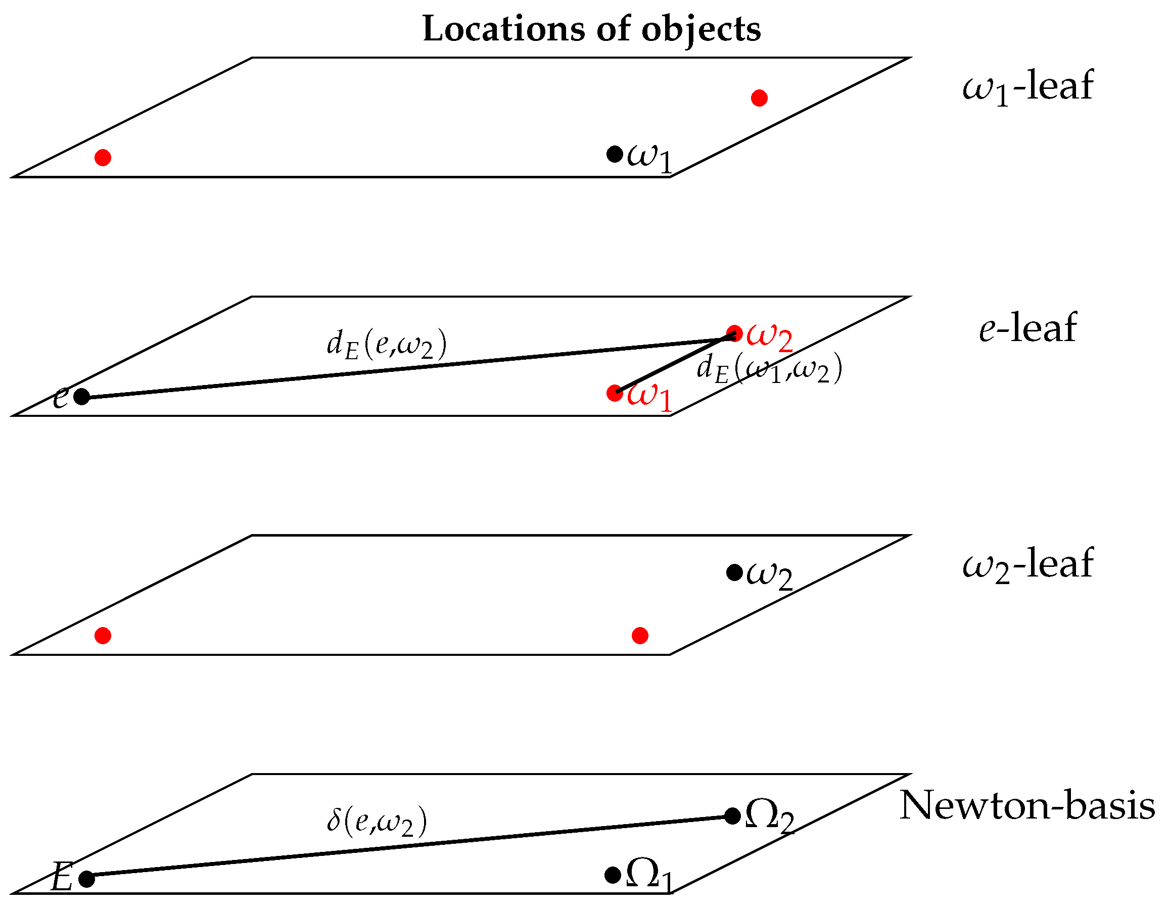
Figure 2.
To sitting-observers, the regions where appear dilated with respect to the regions where . In the case of an inner region with higher the outer region seems to expand (and may generate a gap if has discontinuity), in the case of an inner region with lower the inner region seems to overlap the outer region.
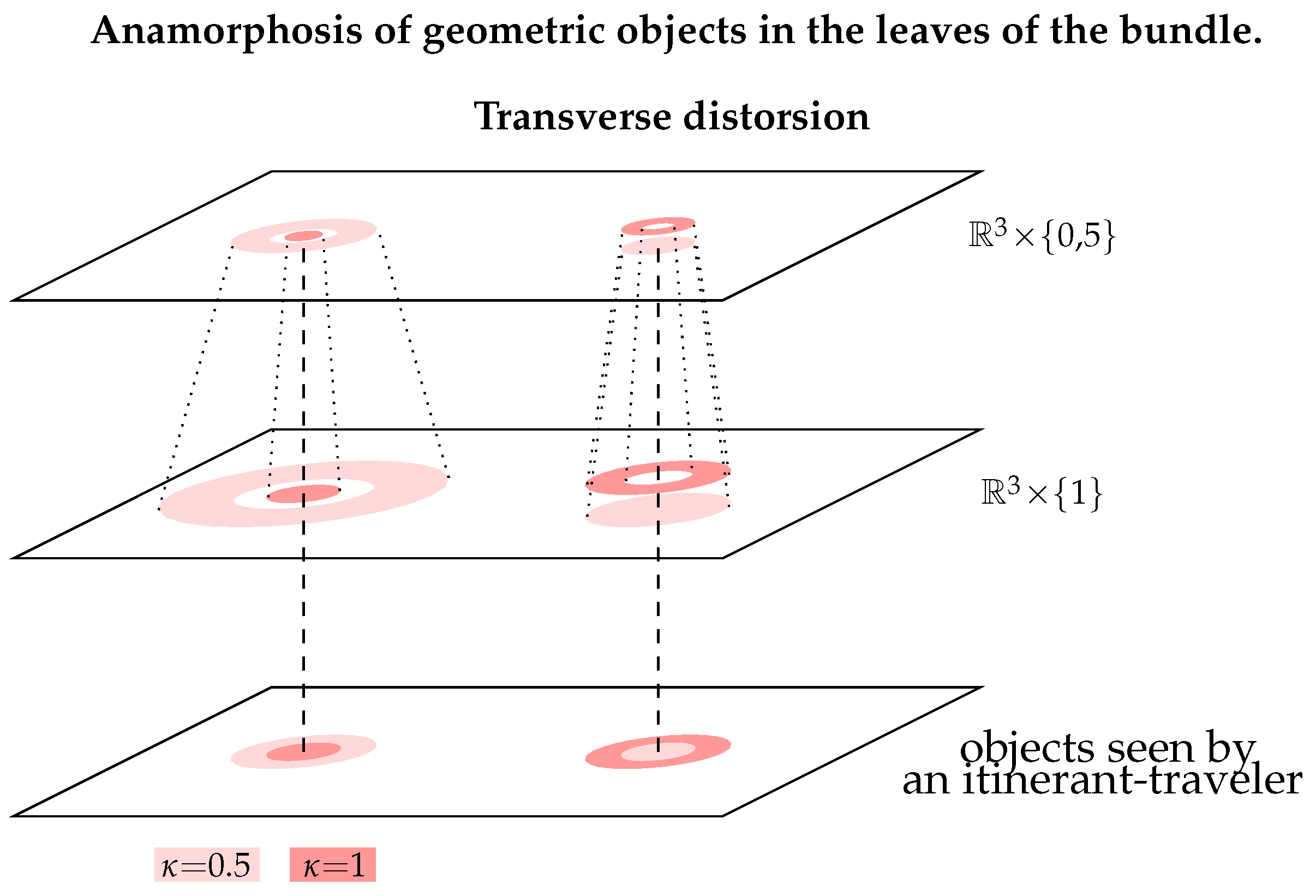
Figure 3.
In shade of blue : density of a galaxy in the Newton-basis. In shade of red : density of its anamorphic counter part in the e-leaf (photometric image). In shade of green : secondary image, (an artificial process, fictitious and non-observable, to construct the photometric image which is fictitious but observable). In shade of orange : the trigonometric image, located behind the photometric image when . From an angular point of view both the photometric and trigonometric images are perfectly superimposed.
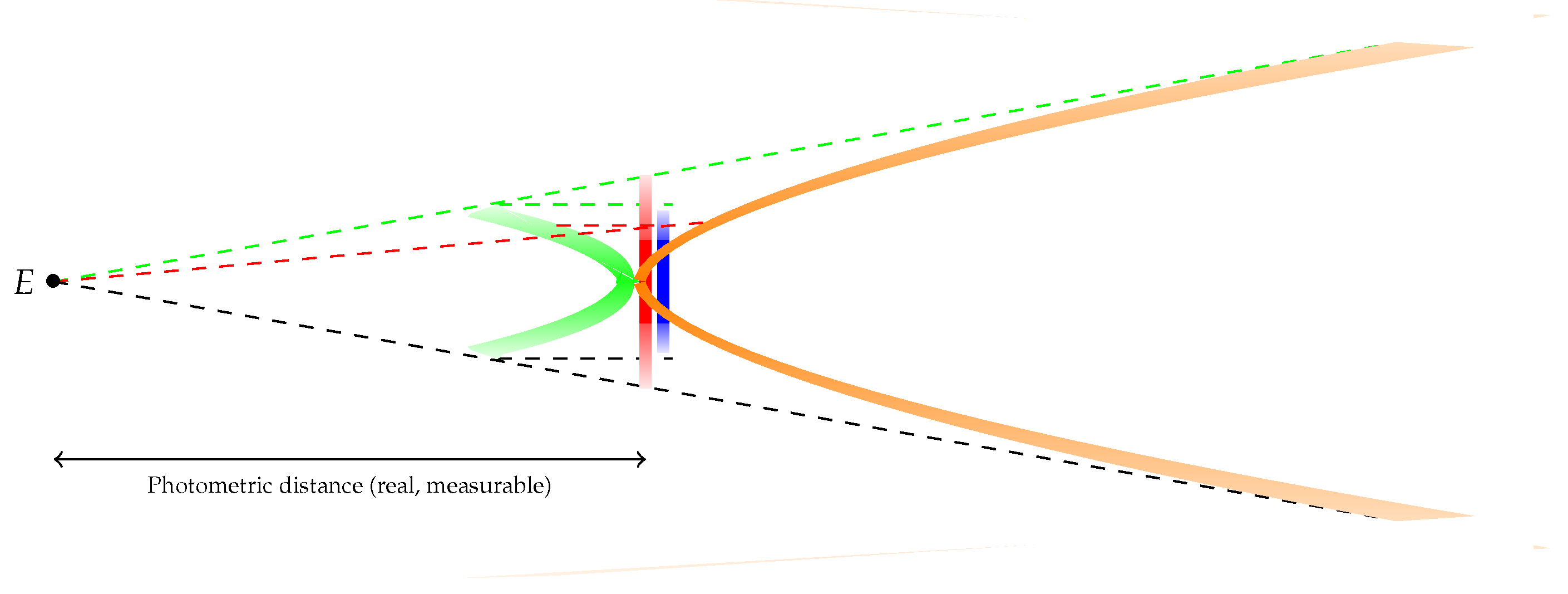
Figure 4.
Areal density profile of the same spiral galaxy seen by three sitting-observers and B at and b with .
Figure 4.
Areal density profile of the same spiral galaxy seen by three sitting-observers and B at and b with .
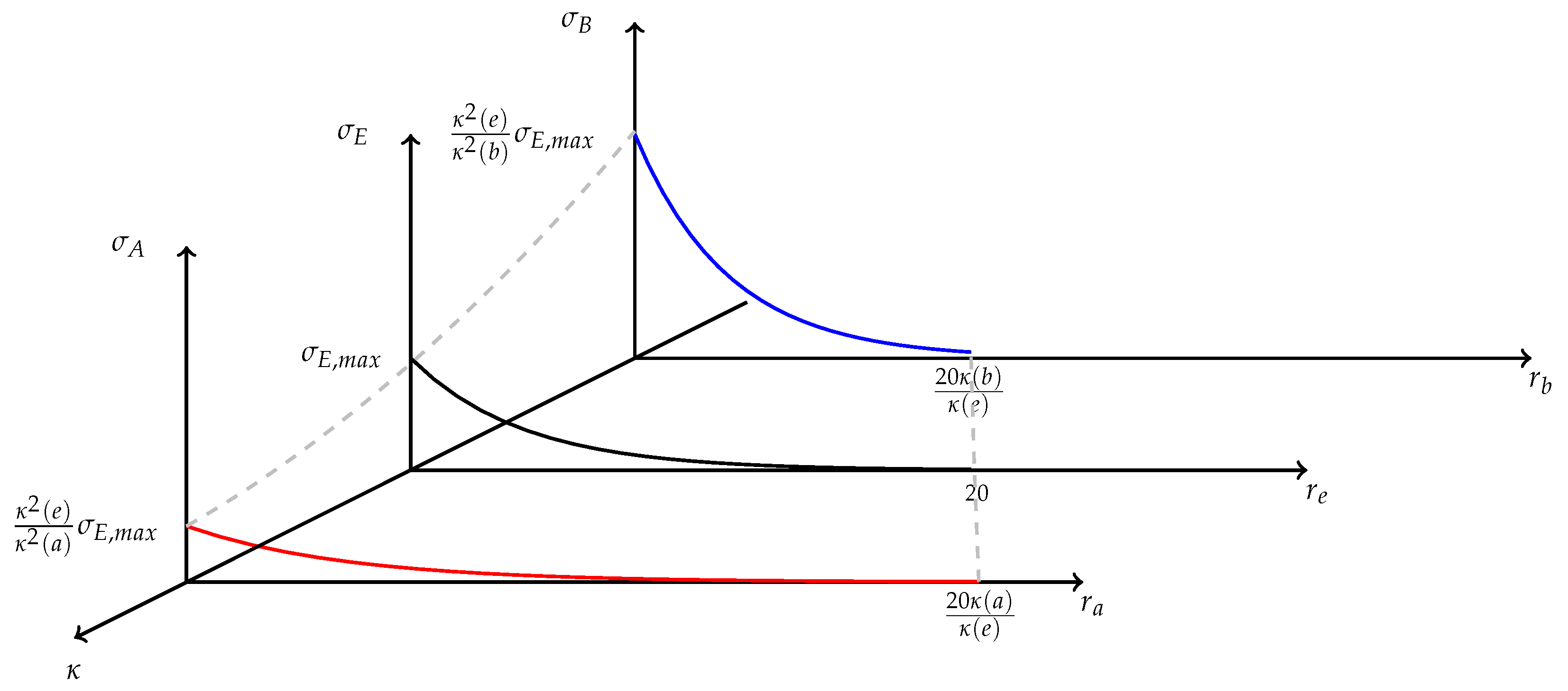
Figure 5.
Mass density in the Newton-basis.
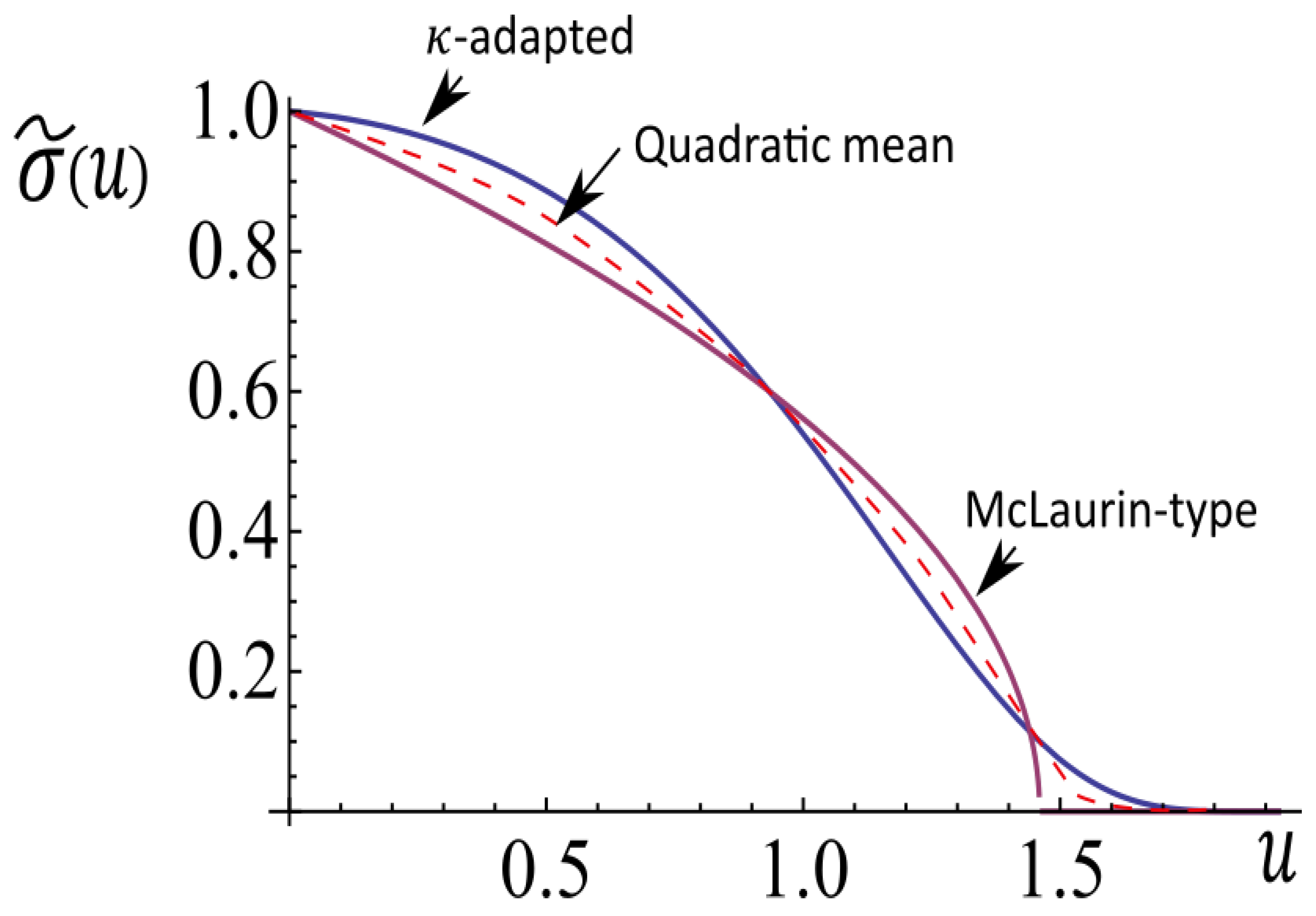
Figure 6.
Velocities profiles.
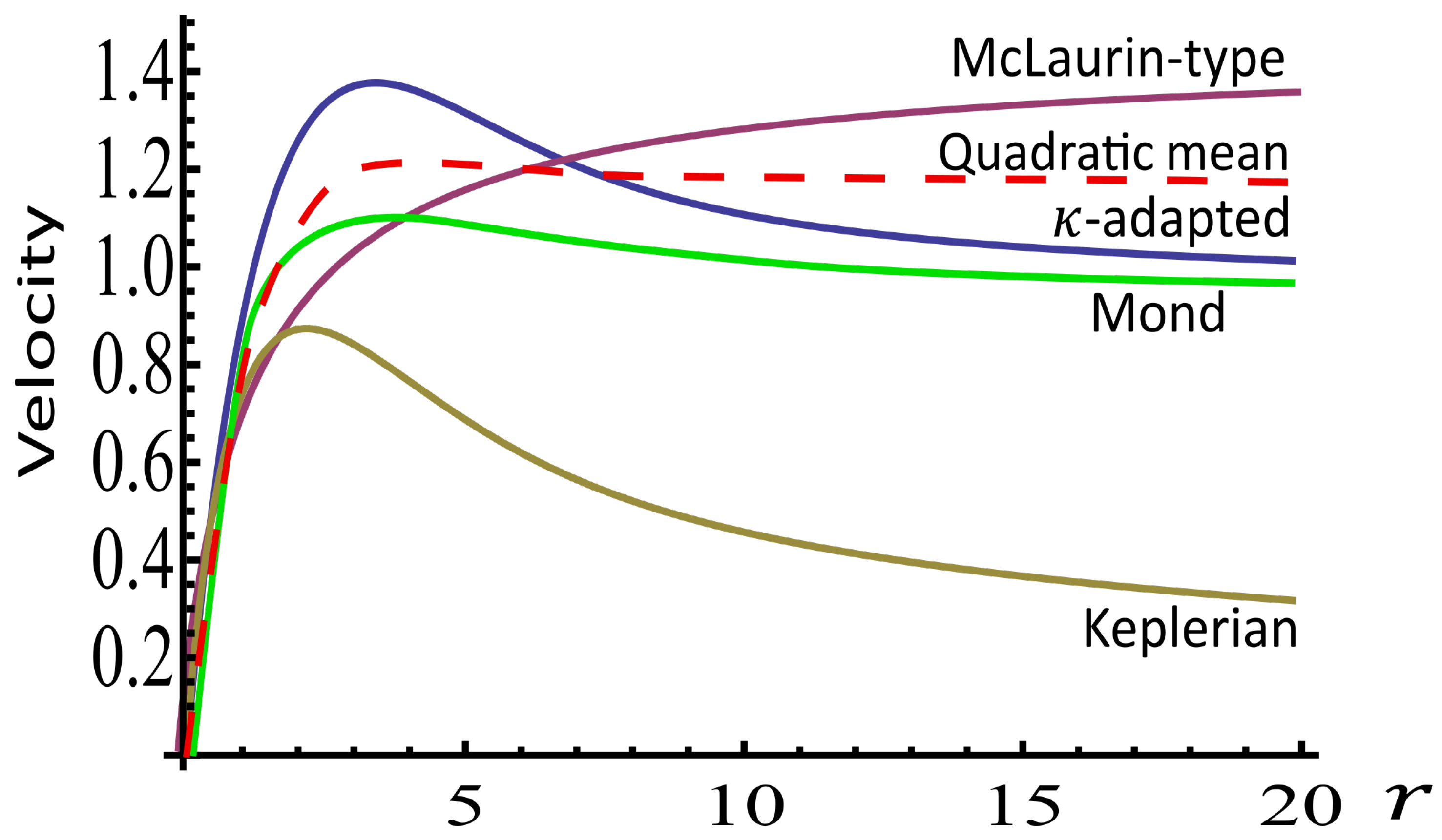
Figure 10.
Representation of a spiral galaxy in the Newton-basis with different inclinations (not observable).
Figure 10.
Representation of a spiral galaxy in the Newton-basis with different inclinations (not observable).
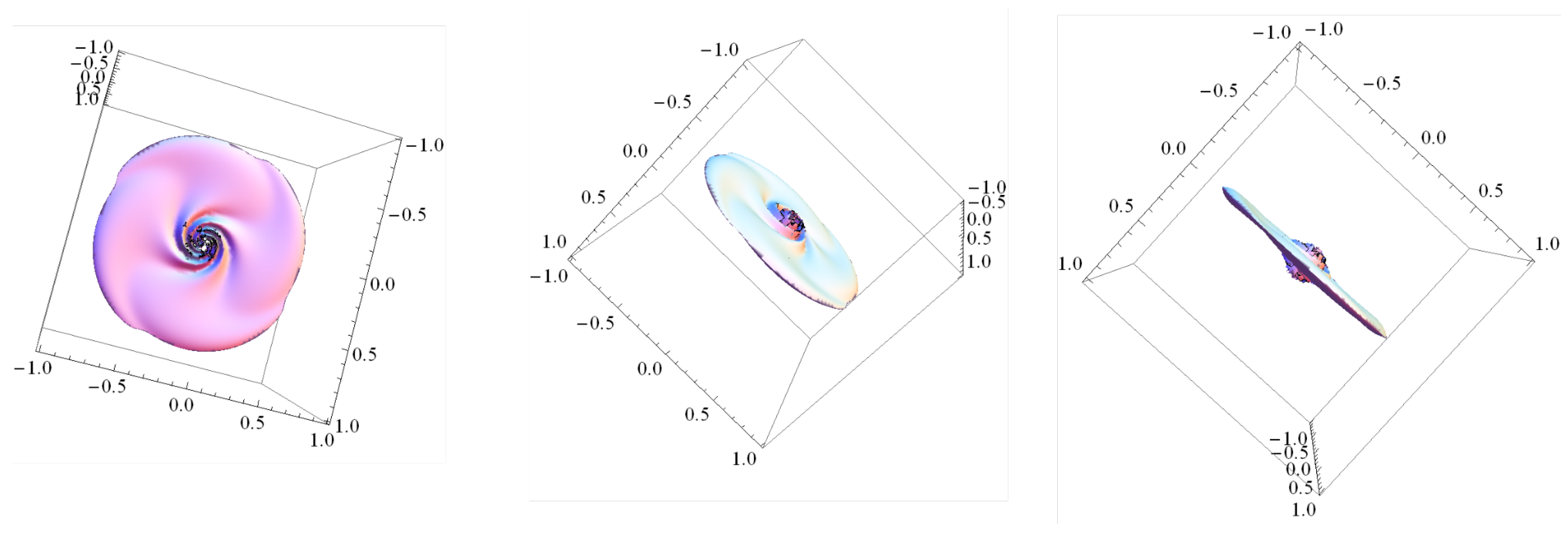
Figure 11.
Visualization of a spiral galaxy in a leaf e.g., by a terrestrial observer. The observed galaxy is obtained by -transport from the Newton-basis.
Figure 11.
Visualization of a spiral galaxy in a leaf e.g., by a terrestrial observer. The observed galaxy is obtained by -transport from the Newton-basis.
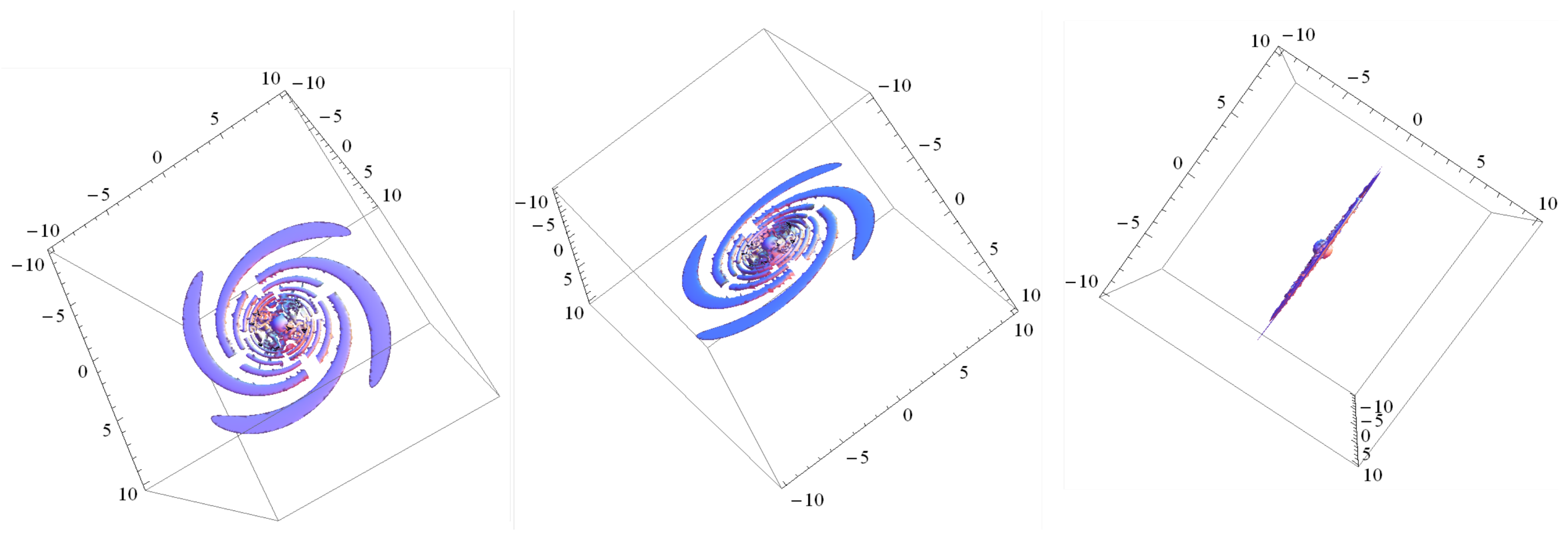
Figure 12.
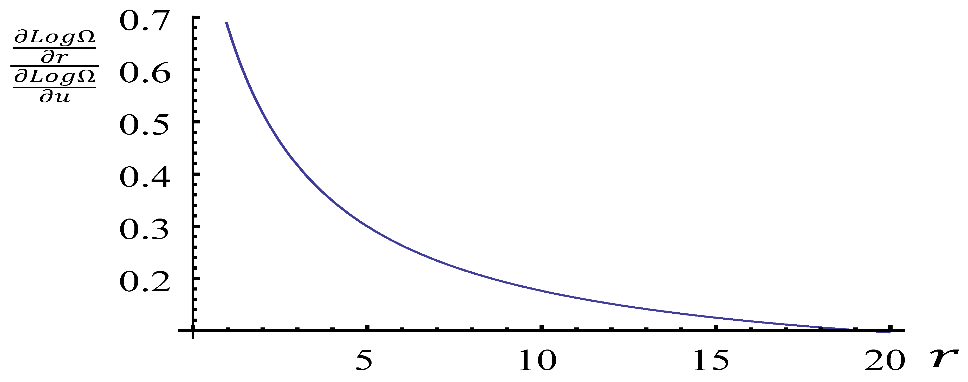
Figure 13.
The velocity v is the spectroscopic velocity.
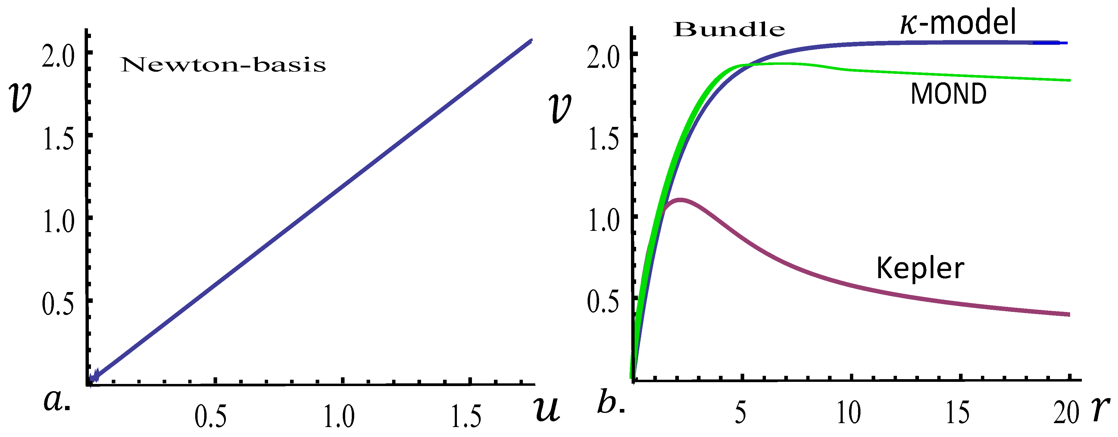
Figure 14.
Observed rotation curve (black circles) of the galaxy M33 is displayed [35] [data 1 Figure 1, data 2 Figure2] together with the theoretical curves predicted by the dark matter model (black line) and (hydro)simulation of MOND [36] (green line). Our added contribution (-model) is represented by the blue line. This is an example where following the observational data (with different inclination and distance) the rotation profile can be fitted better or worse by MOND or -model than dark matter. Another problem is that the receding and approaching side profiles are sensibly different [37,38] (Figure 9). What is the good observational profile?
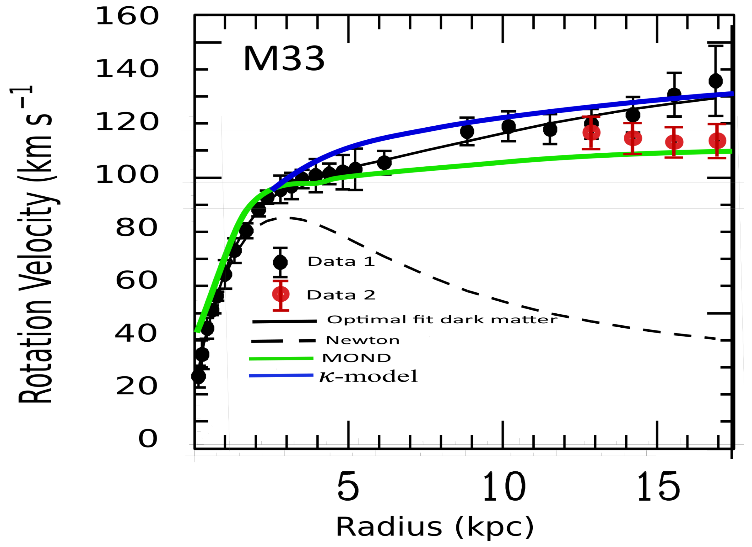
Figure 15.
COMA cluster profile. The horizontal axis is the radius in and the vertical axis is mass in units of the solar mass . The red long dashed curve is the ICM gas mass derived from X-ray observations (compilation of [39,40]); the short dashed blue curve is the Newtonian dynamic mass; the dashed-dotted cyan curve is the MOND dynamic mass; the solid black curve is the MSTG dynamic mass [25]. Our added contribution is displayed as the amber curve, showing the -model dynamic mass with the temperature . The solid green curve displays the -model dynamic mass, assuming a non-isothermal temperature profile (see [7]).
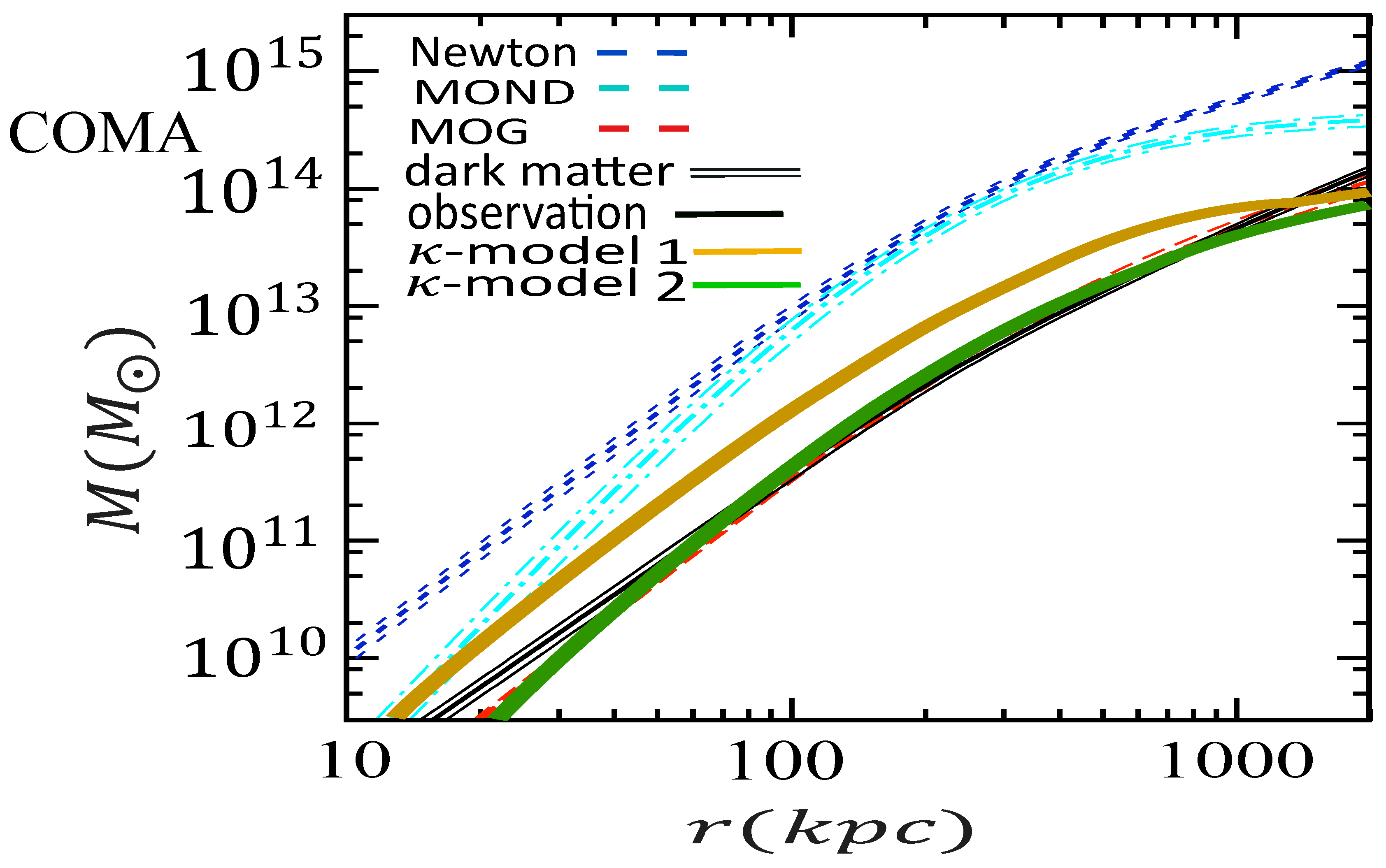
Figure 16.
A comparison between the gravitational lensing diagrams supplied by both the dark matter paradigm and the -model [7]. On the left figure the total weak gravitational lensing is shown. It is the product of the weak gravitational lensing in the basis (the well-known Einstein effect) a The curvature of the photon geodesic initially generated in the Einstein-basis is then strongly amplified in the leaves by -effect (mainly where the mean density is lowest). In addition let us note that the pseudo-Riemannian curvature in the Einstein-basis and the -curvature in the bundle are deeply distinct in nature.
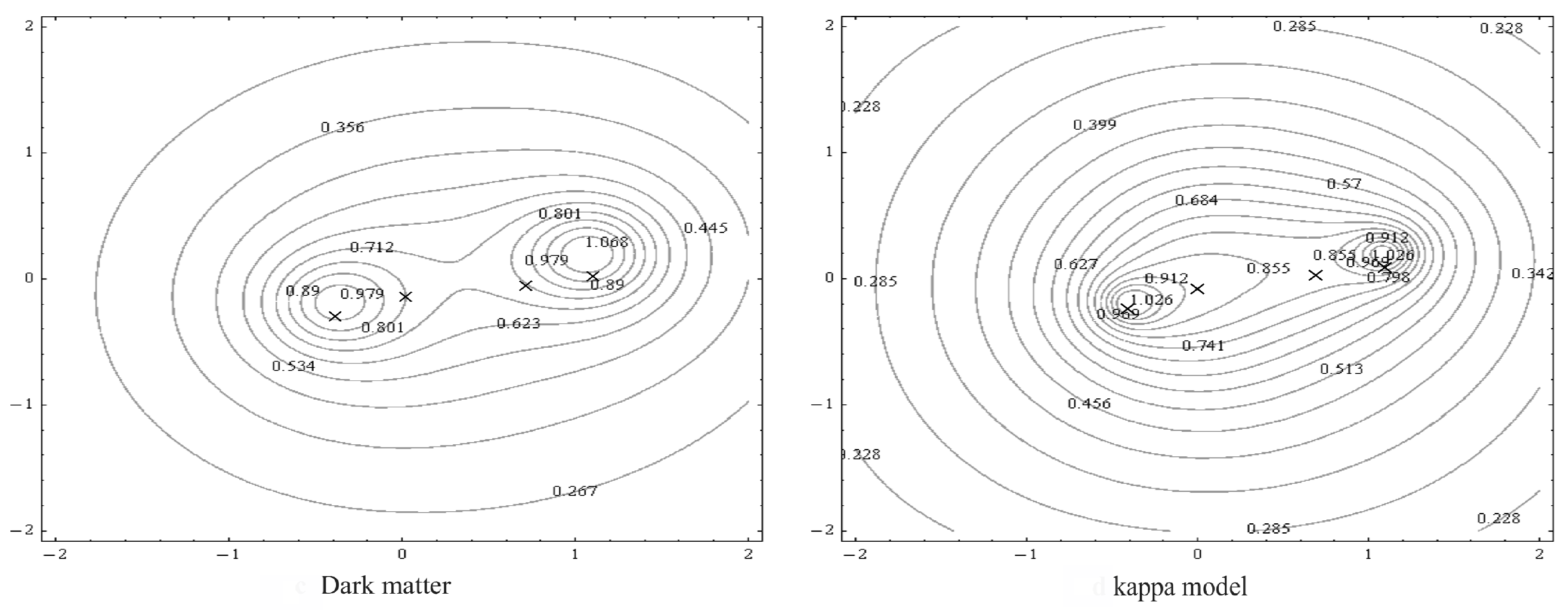
Figure 19.
Hoag’s object in the Newton-basis and as seen by the Hubble Space Telescope.(Image credit : R.Lucas (STScI/AURA),Hubble Heritage Team, NASA)
Figure 19.
Hoag’s object in the Newton-basis and as seen by the Hubble Space Telescope.(Image credit : R.Lucas (STScI/AURA),Hubble Heritage Team, NASA)
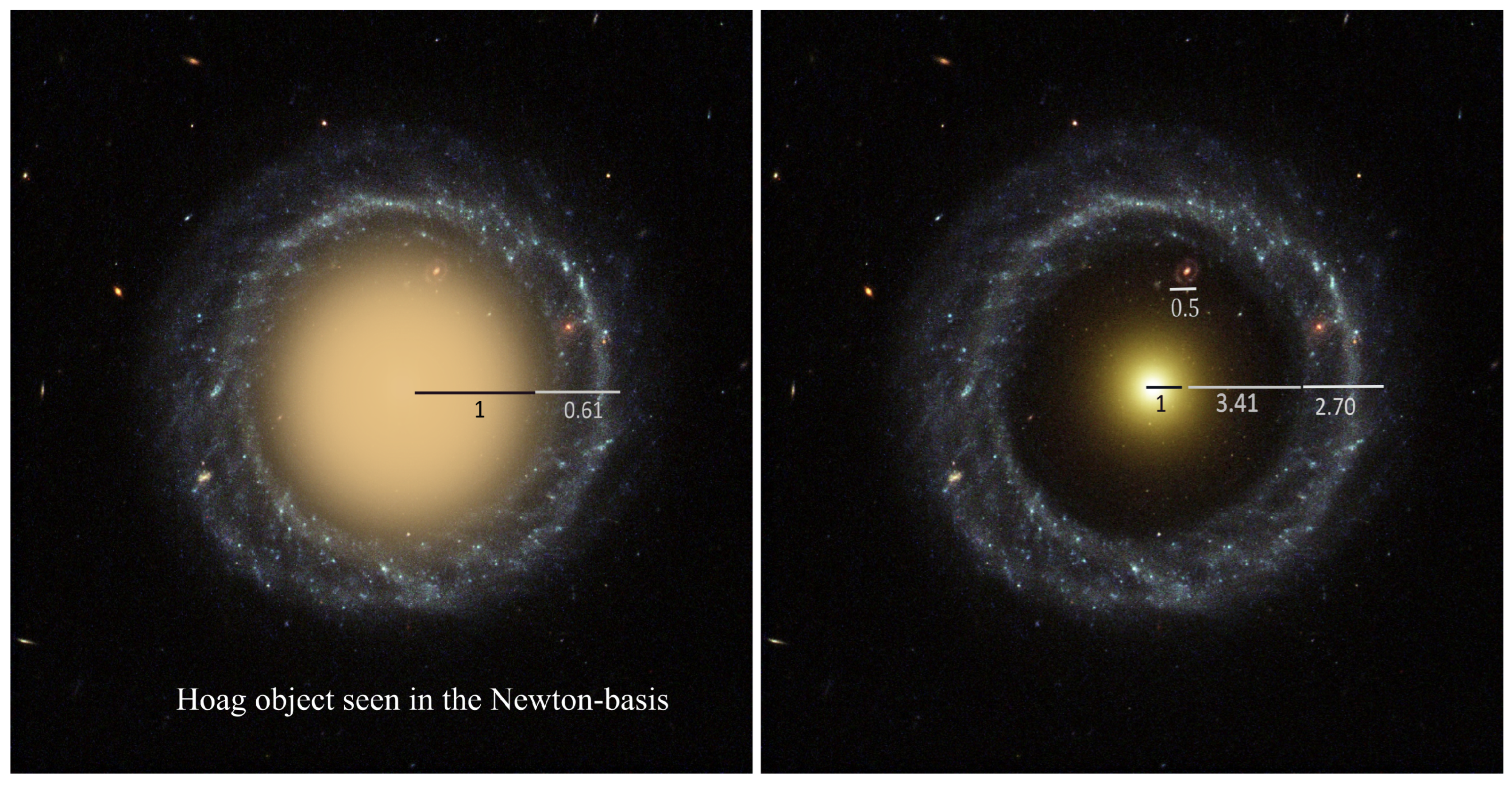
Disclaimer/Publisher’s Note: The statements, opinions and data contained in all publications are solely those of the individual author(s) and contributor(s) and not of MDPI and/or the editor(s). MDPI and/or the editor(s) disclaim responsibility for any injury to people or property resulting from any ideas, methods, instructions or products referred to in the content. |
© 2025 by the authors. Licensee MDPI, Basel, Switzerland. This article is an open access article distributed under the terms and conditions of the Creative Commons Attribution (CC BY) license (http://creativecommons.org/licenses/by/4.0/).
Copyright: This open access article is published under a Creative Commons CC BY 4.0 license, which permit the free download, distribution, and reuse, provided that the author and preprint are cited in any reuse.


