
Submitted:
24 November 2025
Posted:
27 November 2025
You are already at the latest version
Abstract
The aim of the study was the silvicultural assessment of the species composition, structure, sanitary condition, productivity, and carbon content of three modal 120-140-year-old Scots pine forests in the East European forest-steppe of the Russian Plain. Silvicultural, forest inventory and mensuration methods were used to analyze the characteristics of these stands. The distribution models of trees by diameter and growth were analyzed, and the reserves of aboveground and underground phytomass for each forest stand were assessed. All surveyed forest stands are highly productive and in excellent sanitary condition. The forest stand on moist moderately fertile soils was characterized by higher forest mensuration characteristics on average. Allometric relationships between the diameter of forest stands and their height have been established, which will allow mathematical modeling and forecasting of the dynamics of forest stand characteristics in forestry practice. The surveyed forest stands on moderately moist moderately fertile soils store 112.9-122.6 tons of carbon per hectare (tC/ha) in their phytomass, on moist moderately fertile soils - 182.8 tC/ha. About 73% of carbon reserves are concentrated in the above-ground phytomass, and about 27% in the underground phytomass, respectively. Trunk wood accumulates the main part (58-60%) of the aboveground phytomass of the studied pine stands.
Keywords:
pine forests
; species composition
; viability
; carbon content
1. Introduction
In today’s changing environmental and climatic conditions, an urgent task is to monitor the general condition of woody plants, preserve their intraspecific diversity, and study the mechanisms of their adaptation and sustainability. Regular observations of the development of forest communities in test sites or sample plots (SPs) allow us to assess the dynamics of their functioning and determine production of phytocenoses in a changing climate. A phytocenosis is a plant community that forms a stable system with the environment in a homogeneous area. This information is important for understanding the processes that determine the dynamics of phytocenoses, changes in their habitat and biological diversity, as well as modeling the ecosystem processes occurring in them [1,2,3].
Trees in any even aged stand, regardless of their location, usually differ significantly among themselves in a number of forest mensurations: diameter, height, trunk volume, etc. [4]. The structural diversity of tree stands is one of the most interesting phenomena studied by forest ecologists [5]. The study of the structure of the forest cenopopulations is important for understanding the various ecological and biological aspects of their formation. It is also worth noting that the structure of phytocenoses largely determines their productivity and stability [6]. In addition to preserving biodiversity, the young growth and undergrowth can also play an important functional role, regulating natural processes in the ecosystem, for example, by influencing the forest formation process [7], the hydrological regime [8], as well as the cycling of nutrients and carbon [9]. However, at present, the number of studies aimed at the quantitative and qualitative assessment of the understory in pine phytocenoses in the East European forest-steppe is very limited.
A significant number of publications by various researchers have been devoted to the study of pine forests in the East European Forest-Steppe. The sanitary condition and resistance to climate dynamics of natural pine forests in protected areas and in suburban recreational zones have been studied, for instance, in [10,11,12], as well as the growth characteristics, structure, and condition of artificial pine forests, including geographical pine cultures [13,14]. Based on the results of the above-mentioned and other studies, the optimal and most common forest growth conditions in the East European forest-steppe are considered to be moderately moist and moderately fertile soil. In recent years, research has begun on the carbon sequestration function of pine stands [15,16]. Our research continues and deepens knowledge about the structure of natural old-growth pine forests in the region, as well as their carbon sequestration capacity. One of the goals of forest management is to increase forest productivity and resilience, especially in the context of carbon sequestration. Improving the accuracy of modeling and forecasting growth and productivity for a specific ecoregion facilitates effective forest management in a changing climate.
Distribution of trees by forest mensuration indicators - a simple but effective tool for describing the structure of tree populations and stands, which is used to assess wood resources, plan logging operations, and predict forest growth and productivity [17,18,19]. Tree size distribution can also be used to study factors that lead to disturbances in forest ecosystems, as well as to assess aboveground phytomass (live biomass) reserves [20]. The structure of forest stands in forest ecosystems is understood as the regular distribution of trees by forest mensuration indicators that change both in space and time, which is the result of a complex interaction of forest growth conditions, the stage of phytocenosis development, and the history of the influence of exogenous factors.
Traditionally, tree sizes are described by their diameter at a height of 1.3 m or diameter at breast height (DBH), and their frequency distribution is described using probability distribution models. One of the first studies of tree size distribution was conducted by De Liocourt in 1898 [21]. He noted that when representing the distribution of trees in uneven-aged stands by diameter ranges as a frequency histogram it resembles an inverse J-shaped curve. Diameter distribution models are usually based on theoretical distribution functions, such as normal [22], generalized normal, lognormal, beta, Weibull, Johnson’s SB distribution (or “special bounded” distribution), etc. Distribution estimation approaches based on non-parametric methods are also used [23,24,25,26]. Measured stand parameters have a hierarchical structure, and traditional regression models can produce biased results when estimating their parameters and predicting height. Therefore, nonlinear regressions are becoming in-creasingly popular in the development of regional H-D models for pine [27].
Dubenok et al. [28] and Demakova et al. [29] noted that the distribution of trees in even-aged stands by diameter is described by a symmetrical curve, close in shape to a normal distribution. However, since the 1950s, forest scientists have begun to explore models for describing tree diameter distributions (e.g., Meyer [30]), which typically have a right-sided asymmetry. A universal model that can reliably describe all possible tree diameter and height distributions probably does not exist, and there is no consensus on the degree of flexibility a model needs to properly describe the data.
About half of the conifer forests in Russia are classified as mature and over-mature (Box 5.2 in [31]). It was previously believed that mature stands are either carbon emission neutral or release substantial amounts of carbon dioxide (CO2) to the atmosphere [32]. According to [33], the share of carbon in the aboveground and underground phytomass is the highest in mature and overmature pine forests of the Voronezh region, reaching 62% and amounts to 132.8 tC/ha on average. However, according to [34], mature stands continue to actively absorb CO2 from the atmosphere. Therefore, obtaining information characterizing the carbon cycle of old-growth stands growing in various forest growth conditions is still relevant.
The aim of our study was a silvicultural assessment of the species composition of phytocenoses, the structure of tree stands (tree distribution by diameters and heights), the viability (sanitary condition) of tree stands, productivity, and carbon content in modal (most common) 120-140-year-old pine forests of the East European forest-steppe of the Russian Plain.
Silvicultural assessments allow us to determine which forest stands in the study region are the most productive and viable, taking into account observed climate change. Our research also allows us to assess whether silvicultural interventions are required to preserve the studied valuable forest stands, increase their productivity, and enhance their carbon sequestration capacity.
2. Materials and Methods
We studied three SPs (SP1, SP2, and SP3) of Scots pine (Pinus sylvestris L.) in the Voronezh and Lipetsk Regions of the East European forest-steppe of the Russian Plain (Figure 1).
The East European forest-steppe belongs to the zone of highly productive pine forests. It is located on a vast area of the Russian Plain and is heterogeneous in terms of physical, geographical and climatic conditions. Scots pine is the main, indigenous forest-forming species, characterized by high productivity and biodiversity, performing the most important ecological, protective, recreational and other functions, including in the conditions of the East European forest-steppe. When selecting sites for SPs, the ecosystem and intraspecific diversity of natural tree stands in various types of forest growth conditions most common in the East European forest-steppe (on moderately moist and moist gray forest soils) were taken into account. Climate change affects the level of biodiversity in forest ecosystems, but it is biodiversity that underlies the mechanisms by which forests adapt to these changes.
SP1 was established in a natural pine stand with an admixture of oak and birch of less than 5% located in block 60, section 11 of the Left Bank forestry district of the Prigorodnoye forestry district of the Voronezh region (50°84′73″ N, 40°54′27″ E). The relief is flat, the groundwater level is 1-3 m. The average age of the tree stand was 140 years. The size of SP1 is 0.25 ha (50 m × 50 m). The number of trees on SP1 was 60 trees. Forest site type is moderately moist and moderately fertile soil.
SP2 was established in a natural pine stand with an admixture of oak, located in block 65, section 5 of the Left Bank forestry district of the Prigorodnoye forestry district of the Voronezh region (51°81′47″ N, 39°32′59″ E). The relief is flat, the groundwater level is 1-3 m. The average age of the tree stand was 130 years. The size of SP2 is 0.25 ha (50 m × 50 m). The number of trees on SP2 is 78 trees. Forest site type is moist and moderately fertile soil.
SP3 was established in a natural pine stand located in block 124, section 9 of the Balashovsky district forestry of the Gryazinsky forestry of the Lipetsk region (52°30′87″ N, 39°56′42″ E). The relief is flat, the groundwater level is 1-2 m. The size of SP3 is 0.25 ha (25 m × 100 m). The average age of the stand was 120 years. The number of trees in SP3 is 67 trees. Forest site type is moderately moist and moderately fertile soil. Characteristics of SPs are also briefly summarized in Table 1.
The sampling sites in our study represented very well the entire stands, which were very homogeneous regarding topographic conditions, age, site quality, and management regimes. The Central Forest-Steppe stands in Voronezh and Lipetsk regions are located on the Russian Plain (Oka-Don Lowland) with a flat topography. All sample plots are located in protective forests, represent mature stands, have similar forest growth conditions (wet mixed conifer forest), and are of approximately the same age. The sample plots surveyed are representative. Therefore, we believe that the patterns that we identified using relatively limited sample sizes are reliable for such stands.
No forest management activities have been conducted in these stands. Thinning operations end at 60-year-old stands. There is no need for selective sanitary logging in these stands, as they are considered healthy.
A complete count of tree diameters and condition categories was conducted on each SP. The count resulted in the total number of trees on each SP and their distribution by diameters. The diameter was measured at breast height (DBH, ~1.3 m) using a measuring fork. For each diameter category, the height of each tree was measured using an altimeter.
The growing stock was determined using volumetric tables for Scots pine depending on the diameter and height of the trees ([35], pp. 29-30). The composition of the forest stand was determined depending on the share of the stock of each tree species in the total forest stand, which was taken as 100%. If the share of the species in the stock is less than 5%, the presence of the species in the composition is marked with a “+” sign.
The tree density of a forest stand was calculated as the ratio of the sum of the cross-sectional areas of the tree trunks in a forest stand to the sum of the cross-sectional areas of the tree trunks in a normal (standard) forest stand with the same forest mensuration characteristics at a standard density of 1.0 [36].
The trees were categorised and distributed according to the following condition categories: С1 - no signs of weakening, С2 - weakened, С3 - severely weakened, С4 - drying out, С5 - dead [37]. The degree of weakening (condition) of the tree stand on each SP was calculated as the weighted average value of the condition of the tree species (Cm) based on the estimates of the distribution of the trees of different condition categories according to the formula: Cm = (Р1 × C1 + Р2 × C2 + Р3 × C3 + Р4 × C4 + Р5 × C5)/100, where Р1, P2, P3, P4, and P5 are the percentages of trees of each condition category (C1, C2, C3, C4, and C5) in a SP.
The classification of P.S. Pogrebnyak [38] was used to determine the type of forest growing conditions, taking into account the species composition of the forest stand, ground cover, undergrowth species, as well as indicators of soil moisture and productivity. To monitor natural regeneration under the canopy of the forest stand, 10 test sites in size of 2 × 2 m (4 m2) were laid out diagonally at a certain interval in each SP. The test sites were located at the corners of the SPs, where the natural regeneration of each tree species was recorded, with an analysis of the distribution of trees by age and height, and the subsequent transfer of the obtained results to 1 ha. The uccess of natural forest regeneration was assessed according to the scale of V.G. Nesterov (Table 15 in [39], p. 53).
To assess underbrush species, five survey sites in size of 5 × 5 m (25 m2) were laid out on each SP. The total number of trunks (bushes) of underbrush species was counted in each site. The type of underbrush distribution across the plots was determined as group or uneven. Then, the number of trunks was recalculated per 1 ha.
To characterize the ground cover, 10 survey sites in size of 1 × 1 m (1 m2) were laid out on each SP, and the species composition and their percentage were determined on each site. All found ground cover species were grouped according to ecological-cenotic types: forest, forest-meadow, meadow, weed.
To analyze the structure of the surveyed stands by diameter, a normal distribution, Weibull, lognormal and gamma models were used. When processing the forest mensuration characteristics, the following statistical indicators were determined: the arithmetic mean of tree diameter and height, the standard deviation, the error of the arithmetic mean, the variation coefficient, asymmetry, and excess [40].
As a criterion for the statistical significance of differences between the actual observed (ni) and theoretical () number of trees in the ith thickness (diameter) rank, the χ2-square test was used with d.f. = m – 1, where m is the number of thickness ranks: [40]
When comparing the empirical and theoretical distribution curves of heights and diameters, indicators such as distribution asymmetry and kurtosis – the steepness of the distribution compared to the normal one – were analyzed.
Asymmetry was measured using Pearson’s skewness coefficient and calculated using the formula; > indicates right-sided asymmetry, if , then, the distribution is leptokurtic. The excess (steepness of the distribution) was calculated using the normalized moment of the 4th order according to the formula ; > 0 indicates platykurtic distribution, if <0, then, the distribution is leptokurtic [40]. The fitdistrplus program in the R package [41] was used to generate density graphs (distribution of diameters and heights) displaying the density functions of the fitted distribution (Weibull, lognormal and gamma) and the histogram of the empirical distribution.
Cluster analysis following the Ward’s method was used to identify clusters based on diameters and heights.
To assess the quality of the models, the following quality metrics were calculated: the square root of the root mean square error (RMSE), the mean absolute percentage error (MAPE), the mean absolute error (MAE), the mean bias error (MBE), and the coefficient of determination (R2). To calculate the parameters of the Naslund equation when modeling the relationship be-tween tree heights and diameters, the builtin nls (nonlinear least squares) function of the R package was used [42]. Two-parameter nonlinear Näslund model function is given by: [43]
The theoretical distribution of trees according to natural thickness (diameter) grades was calculated using the tables of V.V. Zagreev presented for the Scots pine forest stands in Table 1.1. in [44]. All distributions were tested for correspondence to the observed distributions of empirical data using the Kolmogorov-Smirnov test and χ2 [45].
Regression analysis was used to analyze the relationship between independent variables (predictors, such as stem diameter) and dependent variables (such as tree height). To assess the quantitative relationship between forestry and forest mensuration indicators, the Pearson linear correlation coefficients were calculated [46]. According to M. Dvoretsky (see Table 5.2 in [46]) and to R.E. Chaddock [47], relationships with statistically significant correlation coefficient values up to 0.30 were considered weak, in the range of 0.31-0.50 - moderate, 0.51-0.70 – substantial, 0.71-0.90 - high (tigth), and more than 0.91 - very high (very tigth). The regression model was also assessed using the determination coefficient R2.
To assess the effect of the sanitary condition category on trunk diameter, a one-way analysis of variance (ANOVA) was used, using the F-statistic to assess the significance of differences.
In this study, we considered belowground and aboveground phytomass in the context of carbon storage. The assessment of the aboveground phytomass and its fractions (trunk, branches, and leaves) and belowground phytomass (tree roots) for each tree stand was based on the data on the average trunk diameter at a height of 1.3 m (DBH, cm) and the average tree height (H, m) using the following allometric equation [48]: lnPi = a0 + a1×lnH + a2×lnDBH, where Pi is the dry phytomass in kg of the aboveground parts (trunk, branches, and needles) and roots (respectively Pa, Pst, Pbr, Pf, and Pr); a0, a1, and a2 are species-specific constants of the allometric equation for the tree species and tree parts.
The calculated stocks of aboveground and belowground phytomass (by fractions) were converted into sequestered carbon [48], using the conversion factor of 0.5 recommended by the Intergovernmental Panel on Climate Change (IPCC) for temperate coniferous forests [49]. It was 0.45 for pine needles and 0.5 for other tree parts.
Different conversion coefficients are used for each type of parts, which depends on the forest growth zone. For example, for pine stands, the coefficients depend on the average age, quality and relative density of the stand. To convert phytomass and its parts into carbon reserves, the conversion factors recommended by the IPCC for temperate forests were used: 0.48 for deciduous trees and 0.51 for conifers.
3. Results
3.1. Sanitary Conditions
The assessment of the sanitary condition showed that only trees of the 1st (healthy) and 2nd (weakened) sanitary category were observed in all the SPs. In SP1, the proportion of trees of the 1st sanitary category was 65%, of the 2nd sanitary category – 35%, the average weighted condition category was 1.4. In SP2, the proportion of trees of the 1st sanitary category (healthy) was 90%, of the 2nd sanitary category – 10%, the average weighted condition category was 1.1. In SP3, the proportion of trees of the 1st and 2nd sanitary categories was 50%, the average weighted condition category was 1.5 (tends to be weakened). In all three SPs, there were no trees of the 3rd (very weakened), 4th (drying out) and 5th (dead) sanitary categories. The data are summarized in Table 2.
A one-way analysis of variance (ANOVA) revealed a significant effect of the sanitary category on the trunk diameter in sample plots SP1 and SP3 (F-actual > F-critical). The obtained average trunk diameters for the first and fourth health categories were statistically different (F-actual 6.9 > F-critical 3.8, P < 0.05). In sample plot SP2, no statistically significant differences were found (F-actual < F-critical, P-value > 0.05).
The impact of tree sanitary category on trunk diameter in the SP1 and SP3 sample plots is likely indirect, as severe weakening leading to trunk shrinkage (transition to health category 5) means a cessation of growth in diameter. Trees in sanitary category 1 continue to grow in diameter, while trees with deteriorating health (weakened, severely weakened) may slow their growth.
3.2. Undergrowth
Undergrowth is a young generation of woody plants capable of forming a forest stand in the future. Evaluation of the undergrowth on SP1 showed that it consists of English oak and Scots pine, medium density, up to 5 years old, in quantity of ~5000 pine trees per ha, demonstrating a satisfactory renewal. Oak undergrowth was also present (~200 pine trees per ha), but at SP1 it did not reach the canopy, remaining in a relatively small percentage ratio (~4%) in relation to Scots pine.
On SP2, the undergrowth consists of Norway maple (Acer platanoides L.), oak, and Scots pine of medium density, up to 5 years old, demonstrating a satisfactory renewal for pine with ~6000 trees per ha, while Norway maple (~1000 trees per ha) and oak (~100 trees per ha) were present in a rather smaller amount, and Norway maple did not reach the canopy.
On SP3, the undergrowth consists of pure Scots pine, sparse, up to 5 years old, in quantity of ~4000 trees per ha, demonstrating a satisfactory renewal. On all SPs, pine undergrowth was predominantly small. On SP1, the proportion of small undergrowth trees up to 0.5 m high was more than 60%. The proportion of medium undergrowth by height on this SP1 was 31.5%, large - 8.5%. In SP2, the proportion of small undergrowth was small - only 10%. Medium-height pine undergrowth (up to 2 m) predominates - 85%. Large pine undergrowth was found singly in this SP. In SP3, large undergrowth of Norway maple, 2 m and more in height, predominates, but self-seeding of Scots pine was also found - about 20%. In the studied mature pine forests, the undergrowth of pine species was insufficient to form young pine growth of the next generation. Analysis of the species composition and quantity of underbrush species in the studied sample areas are presented in Table 3.
Red raspberry (Rubus idaeus L.), red elderberry (Sambucus racemosa L.), common rowan (Sorbus aucuparia L.), alder buckthorn (Frangula alnus L.), warty spindle (Euonymus verrucosus L.), common hazel (Corylus avellana L.), and common pear (Pýrus commúnis L) were found in the underbrush of the studied pine forests. The underbrush at SP1 and SP2 was sparse and gathered in clumps. Pine shoots and underbrush were practically absent inside and near the clumps. At SP3 the underbrush was more evenly distributed, its projective cover was about 60%.
The number of understory species varies depending on the type of forest growing conditions, but not dramatically. The largest amount of understory was observed on SP2 (moist moderately fertile soil) with 2760 plants per ha. The species composition, such as common rowan (Sorbus aucuparia L.) and alder buckthorn (Frangula alnus L.) and the number of understory species indicate more humid soil conditions in this area, which is reflected in the larger sizes of pine trees in this area.
3.3. Ground Cover
The types of ground cover in the studied types of forest growth conditions were different. In the type of forest growth conditions with moderately moist moderately fertile soil on SP1 and SP3, the edificator plant was lily of the valley (Convallaria majalis L.), the projective cover of which was about 40% on SP1 and SP3. In the type of forest growth conditions with moist moderately fertile soil on SP2, more moisture-loving plants predominated, such as bracken (Pterídium aquilínum L.), moneywort or creeping jenny (Lysimachia nummularia L.), and the bristly haircap (Polytrichum piliferum L.). The edificator in this area was bracken (Pterídium aquilínum L.), the projective cover of which was 30% (Table 4).
On SP1, about 75% were forest eco-coenotic group plants, including lily of the valley (Convallaria majalis L.), common haircap moss (Polytrichum commune L.), red-stemmed feathermoss or Schreber’s big red stem moss (Pleurozium schreberi L.), wild strawberry (Fragaria vesca L.), common Solomon’s seal (Polygonatum multiflorum L.), and narrow-leaved lungwort or blue cowslip (Pulmanaria angustifolia L.), 25% were meadow eco-coenotic group plants, including bushgrass (Calamagrostis epigejos Roth.) and cow-wheat (Melampýrum pratense L.) (Table 5).
On SP2, the forest eco-coenotic group includes common haircap moss (Polytrichum commune L.), bracken (Pterídium aquilínum L.), bristly haircap (Polytrichum piliferum L.), false lily of the valley or May lily (Maianthemum bifolium L.), pipsissewa or umbellate wintergreen (Chimáphila umbelláta L.), and common clubmoss or running clubmoss (Lycopodium clavatum L.), making up 67% of the total ground cover. The forest-meadow ground cover on this site includes round-leaved wintergreen (Pyrola rotundifolia L.), and the meadow ground cover includes bushgrass (Calamagrostis epigejos Roth.) and moneywort or creeping jenny (Lysimachia nummularia L.). On SP3, the forest eco-coenotic group of plants makes up about 40% and includes lily-of-the-valley (Convallaria majalis L.), red-stemmed feathermoss or Schreber’s big red stem moss (Pleurozium schreberi L.), and wild strawberry (Fragaria vesca L.). The forest-meadow eco-coenotic group on this SP was also represented by Sidebells wintergreen (Orthilia secunda L.). The meadow eco-coenotic group of plants makes up about 50%, including cow-wheat (Melampýrum pratense L.), Bloody cranesbill or bloodred geranium (Geranium sanguineum L.), yellow bedstraw or Lady’s bedstraw (Galium verum L.), and corn speedwell (Veronica arvensis L.). Comparison of eco-coenotic groups showed that the forest group was dominant, regardless of the type of forest growth conditions. A greater number of plant species in the living ground cover was observed on SP2 with moist moderately fertile soil.
According to numerous studies [10-14, etc.], forest growth conditions with moderately moist and moderately fertile soil were considered optimal for pine growth in the East European forest-steppe. However, under the observed climate change conditions, we see that stands with moist and moderately fertile soil exhibit the best characteristics of condition, productivity, and carbon sequestration.
3.4. Diameters and Heights
To identify the cenotic structure and allometric dependencies of tree height from diameter in the surveyed stands, we analyzed the main characteristics of the stand – distribution of trees by diameters and heights. Individual height and diameter values for each tree and sample plot are presented in Table S1. The data were calculated on the basis of regional tables developed by V.V. Zagreev and presented for the Scots pine forest stands in Table 1.1. in [46].
The diameters of pine trees at different SPs varied from 22 ± 0.15 cm at SP3 to 64 ± 0.5 cm at SP2. At SP2, there was a large variability in the diameters of individual trees, which was due to the presence of small-sized trees, although their number was small. Statistical parameters of the tree diameters and heights at the SPs are presented in Table 6.
On SP2, the average diameter of pines was higher than on SP1 and SP3, but the average diameters of all the SPs surveyed were within two adjacent thickness ranks.
The coefficient of variation (CV) of height ranged from 15 to 24% among the SPs. Height asymmetry was insignificant – from -0.13 to -0.36, indicating a normal distribution of trees by height. Negative values of height asymmetry indicate an excess of tall trees. The histogram of tree height distribution, and Weibull, lognormal, and gamma distributions for sample plots SP1, SP2, and SP3 are shown in Figure 2.
According to χ2 and λ, the observed distributions of tree heights in the SP1, SP2, and SP3 did not differ significantly from the expected normal distribution.
One of the main indicators of the forest stand structure is the distribution of trees by diameter. The average trunk diameter was 42.2 ± 0.1 cm in SP1 and 41.0 ± 0.3 in SP3, but the largest - 48.5 ± 0.2 cm - was in the overmature pine forest at SP2 (Table 6). Histogram of tree diameter distribution, and Weibull, lognormal, and gamma distribu-tions for sample plots SP1, SP2, and SP3 are presented in Figure 3.
The coefficient of variation (СV) of diameter varied from 27 to 36% in the studied SPs, which indicates a large stretch of the tree distribution curve for this trait. A small asymmetry in diameter, close to zero (-0.03), was noted on SP3, which indicates a close to normal distribution of trees for this trait, while moderate asymmetry was observed on SP1 (0.21) and SP2 (-0.45).
According to χ2 and λ, the observed distributions of tree heights in the SP1, SP2, and SP3 did not differ significantly from the expected normal distribution.
We calculated the theoretical distribution of tree diameters and compared it with the observed one for each SP using the Pearson χ2 and Kolmogorov–Smirnov (D) tests. It turned out that by both tests the theoretical distribution was significantly different from the observed one in SP2 (χ2 = 12.8, P < 0.05; D = 0.45 > Dcritical = 0.20 for a=0.05), but did not differ in SP1 (χ2 = 6.0, P > 0.05; D = 0.13 < Dcritical = 0.17 for a=0.05) and SP3 (χ2 = 3.8, P > 0.05; D = 0.11 < Dcritical = 0.16 for a=0.05).
For the empirical and theoretical distribution functions, the calculated RMSE, MAE, MBE metrics show that the Weibull distribution demonstrates the best alignment result (Table 7).
Based on the accumulated ranks for the quality metrics under consideration, the smallest discrepancies between the actual and model-calculated root-mean-square diameter values were obtained for the normal and Weibull distributions. The normal and Weibull distributions are characterized by slightly underestimated values (MBE > 0), while the lognormal distribution is characterized by overestimated root-mean-square diameter (MBE < 0).
Cluster analysis by diameters and heights (single linkage method, complete linkage method, Ward’s method, etc.) did not reveal any significant clusters among the surveyed stands, despite differences in the types of forest growing conditions (moderately moist moderately fertile soil and moist moderately fertile soil), thus confirming the significant similarity and comparability of the studied stands according to silvicultural and forest mensuration characteristics.
The relationship (correlation) between the height and diameter of trees was also analyzed. As the tree height increased, its diameter and the CV of diameter increased, but the CV of height decreased. The CV of height directly depended positively on the number of trees per a ha and negatively on the tree diameter in all SPs (Table 8).
A direct linear correlation was established between the trunk diameter and the tree height with high and significant correlation coefficients (r) equaled 0.81 in SP1, 0.86 in SP2 and 0.84 in SP3. The two-parameter nonlinear Näslund model has the best predictive power, as it allows for the prediction of an individual height curve for each individual stand. Table 9 presents the Näslund equations with parameters b1 and b2 for SP1, SP2, and SP3.
The best model reflecting the dependence of tree height on trunk diameter at a height of 1.3 m from the ground surface for Scots pine stands is the two-parameter Näslund function. It was found that the regression value (R2) between tree height and diameter varied from 0.92 to 0.96. The highest R2 value (0.96) was found for trees on SP2 (Table 9).
All parameter estimates and model variance components are highly statistically significant (p < 0.001; Figure 4). The Näslund model more accurately predicts the relationship between tree height and trunk diameter compared to the linear allometric relationship.
3.4. Aboveground and Underground Phytomass Reserves
Using allometric equations (based on data on average tree diameters (D) and heights (H)), we calculated the reserves of aboveground and underground phytomass (in kg of fresh weight) per average tree in the surveyed stands: lnPst = -3.2484 + 2.3927×lnH + 0.7586×lnD, R2 = 0.981; lnPbr = -3.5496 + 1.3197×lnH + 1.7788×lnD, R2 = 0.942; lnPf = -2.6645 + 0.8007×lnH + 1.748×lnD, R2 = 0.910; lnPa = -2.3633 + 2.042×lnH + 1.0193×lnD, R2 = 0.968; lnPr = -3.9142 + 1.9909×lnH + 0.9533×lnD, R2 = 0.951; where Pst, is phytomass of trunks, Pbr - phytomass of branches, Pf - phytomass of needles, Pa - phytomass of the aboveground part, and Pr phytomass of roots.
Then the obtained data on phytomass in kilograms per average tree were converted into tons with subsequent multiplication by the total number of trees in the surveyed stand (based on the measurement data on the sample plot). The phytomass reserves in the three surveyed sample plots are presented in Table 10.
The timber volume was 450 m3/ha, and the total phytomass was 245.5 t/ha on SP1 (moderately moist and moderately fertile soil). The aboveground phytomass consisted mostly of wood in the studied pine forests with trunks accounting for 60.5% of the total phytomass (Table 10). With age, the share of this fraction in the total phytomass of the tree layer increases [50].
The timber volume was 420 m3/ha, and the total phytomass was 244.9 t/ha on SP3, growing on moderately moist, moderately fertile soils identical to the first trial plot. Trunks accounted for 58% of the total phytomass (Table 10).
The highest timber volume (490 m3) and the total phytomass (365.8 t/ha) were on SP2, growing on moist, moderately fertile soils.
Based on the aboveground and underground phytomass, the carbon stocks in the studied forest stands were calculated using the conversion coefficient 0.5 and presented in Table 11.
The examined 120 and 140-year-old pine stands on moderately moist moderately fertile soils stored 112.9 and 122.6 tC/ha in their phytomass based on the SP3 and SP1 data. The 130-year-old stand on moist moderately fertile soils stored 182.8 tC/ha based on the SP2 data, with almost all the carbon accumulated in the pine trunks. About 73% of the carbon reserves were concentrated in the aboveground phytomass, and about 27% in the underground phytomass, respectively.
4. Discussion
The growth and productivity of forest stands are among the most important indicators of their condition. In the context of ongoing environmental changes, the increasing role of forest ecosystem functions, the need to increase the productivity of forest stands considering an increasing deficit of wood raw materials, the importance of assessing these indicators is constantly increasing. At the same time, the development of new and improvement of existing standards and models of forest stand dynamics is also of great importance for the successful solution of many forestry problems.
The species composition of 120-140-year-old pine stands determines their viability, because they are the basis of these forest ecosystems. Pine stands as the main component are an indicator of the viability and productivity of the forest stand as a whole.
According to [51], the living ground cover, understory, and young growth participate in the minor biocycle, maintain soil fertility, protect the soil from leaching and salinization, and, accordingly, have a fundamental influence on the future formation of highly productive coniferous stands. According to [52], the average stand density has a significant impact on the species richness of the shrub and herb layers. The study [53] examined the relationships between the abundance of ponderosa pine, the canopy environment, and the species composition of the understory. It was found that the occupancy of ponderosa pine is inversely proportional to the abundance of perennial bunchgrasses in the under-story and species diversity. Many researchers have identified diversity, variation and changes in the amount of undergrowth and living ground cover, depending on the species and age of trees, stand density and forest types [54,55,56].
The developed generalized model of tree diameter distribution in pine stands, combined with models of tree height dependence on trunk diameter, can serve as a useful tool for forest management, making it possible to determine the structure of the growing stock. Early models of tree trunk diameter frequencies used the root-mean-square diameter for forecasting, which is one of the main indicators of forestry stands. In recent years, interest in the root-mean-square diameter as an indicator for forecasting tree diameter distribution has increased [57,58,59]. Some studies [60,61] emphasize that empirical models should not be complex, especially if their purpose is to be used in forestry practice rather than in scientific research. The generalized model we obtained meets this requirement. Maltamo et al. [62] note that there are no mathematical, and especially biological, grounds for assuming any theoretical distribution of tree trunk diameters.
The trunk diameter at a height of 1.3 m (DBH) is the main predictor used to infer the height and size of trees [63,64]. The analysis of the values of heights and diameters and their distribution on the surveyed SPs allowed us to conclude that these easy-to-measure forest mensuration parameters can be used in the preliminary assessment of bioecological diversity for further genetic selection. The results of our study are consistent with domestic [65] and international [66] practices of applying regression models to predict height with known values of tree trunk diameter. The Näslund models of height-to-trunk diameter dependence derived by us can be included as a separate component in simulation models of forest stand growth and productivity, where they form the basis for determining the timber stock, its commercial structure, and biological productivity. Our data are also consistent with the data of [67,68]. Ou et al [69] used nonlinear modeling to model the height-to-diameter-at-breast-height (DBH) dependence for Durango pine. Lin et al [70] compared the approximating ability of six models in their article while modeling height-to-diameter models for Mongolian pine (Pinus sylvestris var. mongolica). Generalized and basic nonlinear regression models performed best because random-effects calibration provided the lowest height prediction bias.
The Näslund model serves as an alternative to the rank tables used in forest inventory, which show conventional relationships between height and tree trunk diameter. It allows for height calibration based on 3–5 measurements of tree height and trunk diameter in the studied stand. The Näslund computing processes are often more simple, stable, and efficient than those of the than other models [71,72]. Using the model increases the accuracy of timber stock determination in Scots pine stands of the East European Forest-Steppe.
Of greatest interest to researchers are the models of the relationship between tree heights and their DBH [73].
In the 2000s–2020s, there was increased interest in the use of regression models to study the processes of growth and increment of tree stands [74]. Generalized models are actively used to approximate the effect of the trunk diameter on tree height [75]. These models allowed us to obtain values of tree height in a stand based on diameter values. Measuring the DBH is simpler, more accurate and cheaper than measuring the height of a tree [76]. Studies [77] carried out for stands of Turkish or Calabrian pine (Pinus brutia Ten.), Austrian or black pine (Pinus nigra J. F. Arnold), and Lebanese cedar (Cedrus libani A. Rich.) in southern Turkey showed that the height-diameter models differed significantly for different ecological regions. The authors concluded that to improve the accuracy of forecasting, such models should be developed for individual ecoregions. The development of such models of forest growth and productivity is supported by data from long-term observations in sample plots and assessments of the effects of climate change, which also serve as the basis for forest management [78,79]. Silvicultural models of different spatial resolutions (region, stand, individual-oriented) have been successfully used to assess various forest management regimes and make economic calculations [80]. Models based on tree height and diameter data are used to solve various forest management problems: forecasting stand growth, modeling thinning regimes, analyzing stand dynamics, or assessing forest productivity. Thus, the Forecast model [81] includes economic assessments and has a developed user interface. The MOTTI model [82] is included in the MELA decision support system in Finnish forestry [83]. However, many silvicultural models have limited applicability due to a lack of experimental data [84]. Most models do not take into account the influence of climate as a factor determining forest dynamics, so they are not used to analyze the consequences of climate change [85]. In Russia, the most widespread is the simulation model for forecasting the dynamics of mixed stands of different ages and the FORRUS-S (FORest of RUSsia – Stand) software suite developed on its basis, which is designed for simulation modeling and analysis of dynamic processes occurring in forest areas [86].
Previous studies of the viability and productivity of modal pine forests [15] also noted their high viability and productivity. A study of the allometric relationships between diameter and height in the Central Forest-Steppe has not previously been conducted. Ac-cording to data from [28], 28 simple regression relationships between tree height and trunk diameter at a height of 1.3 m were analyzed for pine forest plantations in the Moscow region (Russia), and it was found that the simplest and most universal of the models is the two-parameter Neslund model. We found that this model is also the best for the Central Forest-Steppe.
The main characteristic of forest ecosystems is biological productivity [87]. In the current conditions of depletion of forest raw materials, the need for rational use of forest wood resources is most acute. This problem can be solved with high-quality and complete forest inventory information, up-to-date databases that can be supplemented and improved by using mathematical models that adequately describe the dependence of bioproductivity parameters on simple forest mensuration indicators. In this case, preference is given to simplified models that are accessible for analysis [88]. The regression method allows us to successfully predict the development of trees and the formation of trunks [89]. Most forest inventory standards mainly assess the resources of stem wood. However, new challenges, in particular from the perspective of the forest climate agenda, make it necessary to have models and data on the bioproductivity of forest stands that allow us to take into account the fractional assessment of the dynamics of accumulation of living organic matter, carbon deposition, and net primary production of forest stands [90]. Predictive assessment of the biomass of various parts (fractions) of trees allows economically justified and rational use of tree greenery, bark and wood itself, which, for example, determines the profitability of the first thinning techniques and clearing of burnt areas. The relevance of phytomass research is constantly increasing in our time [91,92,93,94].
The study of the productivity of phytomass, the features of its formation in connection with microclimatic and hydrological conditions is of considerable importance, since the processes of soil formation, the stability of plantings and the preservation of their protective functions directly depend on the dynamics of phytomass accumulation. The essence of biogeocenotic processes and the specificity of the reproduction of organic mass in plant communities is manifested, first of all, in the structure of phytomass and its quantitative expression. It is the reserves of phytomass that reflect the features of the development of plantings [95]. Lukina et al. [96] attribute physical, chemical and biological events or actions that link organisms and their environment, such as biomass production, decomposition of litter, and cycles of nutrients, to ecosystem processes in the forest. In the forest phytocenosis, which is the most important component of the forest biogeocenosis, biological productivity characterizes the rate of formation and accumulation of organic matter in the form of phytomass.
According to the data provided by Rock et al. [97], the decomposition constants of pine wood, depending on the region of growth, vary from 0.01 to 0.07 per year, with an average of 0.04 per year. The authors noted that the use of decomposition constants from public sources allows for a fairly accurate description of carbon losses during the decomposition of large wood residues. For European boreal forests, Shorohova and Kapitsa [98] provided information that the decomposition rate of wood of different species varies on average from 0.014 (pine) to 0.071 (spruce) per year.
5. Conclusions
Of great importance is the analysis of the state of all components of the phytocenosis of old (120-140 years) natural pine modal forest-steppe stands, since they form the ecological basis of the region and determine both carbon deposition and all the main environment-forming functions. In accordance with this, we assessed the viability and productivity of such stands, which, in turn, determines their carbon deposition function.
Analysis of the species composition of the ground cover, undergrowth and young growth in the surveyed SPs showed a high similarity of tree stands growing on moderately moist and moderately fertile soils. The forest stand on moist moderately fertile soils (SP2) is characterized by higher average forest mensuration characteristics (trunk diameter - 48.5 cm, tree height - 29 m), as well as the presence of more moisture-demanding ground cover species, such as bracken (Pterídium aquilínum L.), moneywort or creeping jenny (Lysimachia nummularia L.), and bristly haircap (Polytrichum piliferum L.), and underbrush species, such as common rowan (Sorbus aucuparia L.) and alder buckthorn (Frangula alnus L.). All surveyed forest stands were highly productive an in excellent sanitary condition with the weighted average value of the condition category, varying from 1.1 for SP2 to 1.5 for SP3. Until now, moderately moist and moderately fertile soils were considered optimal for pine growth in the East European forest-steppe. However, we have found that under current climate change, stands with moist and moderately fertile soils exhibit the best health, productivity, and carbon sequestration characteristics.
We have established allometric relationships between diameter and height for the surveyed stands, based on which mathematical modeling of height by diameter of the surveyed stands was carried out that will improve the accuracy of forecasting the growth and productivity of pine and the effectiveness of forest management in the East European forest-steppe.
Old-growth forests are good repositories of carbon deposited from the atmosphere. In the 120-140-year-old pine stands that we surveyed, the carbon content in the pool of aboveground and underground phytomass was highest in the stand growing on moist moderately fertile soils (SP2) - 182.8 tC/ha.
As our study has shown, additional forestry measures are not required to preserve the studied valuable forest stands and increase their productivity.
Supplementary Materials
The following supporting information can be downloaded at the website of this paper posted on Preprints.org, Table S1: Individual height and diameter values for each tree in sample plots SP1, SP2, and SP3.
Author Contributions
Conceptualization, S.M.M. and D.A.L.; methodology, S.M.M. and D.A.L.; software, A.V.M. and D.A.L.; validation, S.M.M., D.A.L., A.A.P. and K.V.K.; formal analysis, S.M.M., D.A.L., A.A.P. and K.V.K.; investigation, S.M.M. and D.A.L.; resources, S.M.M., D.A.L. and A.V.M.; data curation, S.M.M.; writing—original draft preparation, S.M.M., D.A.L.; writing—review and editing, S.M.M., D.A.L. and K.V.K.; visualization, S.M.M., D.A.L., A.V.M., A.A.P.; supervision, S.M.M.; project administration, S.M.M.; funding acquisition, S.M.M. All authors have read and agreed to the published version of the manuscript.
Funding
This research was funded by the Russian Science Foundation grant No. 24-16-20047 “Population structure and intraspecific variability of dendrophenotypes of Scots pine and pedunculate oak as the basis for adaptive resistance to climate change and other external influences”.
Data Availability Statement
The original contributions presented in this study are included in the article. Further inquiries can be directed to the corresponding author.
Conflicts of Interest
The authors declare no conflicts of interest.
Abbreviations
The following abbreviations are used in this manuscript:
| CO2 | Carbon Dioxide |
| CV | Coefficient of variation |
| DBH | Diameter at breast height |
| SP | Sample plot |
References
- Mapitov, N.B.; Zhumadina, S.M. Tree–Ring Analysis of Radial Increment of Pinus Sylvestris L. in Shalday Pine Forests in The Northeast of Kazakhstan. Res. J. Pharm. Biol. Chem. Sci. 2016, 7, 180–187. Available online: https://www.rjpbcs.com/pdf/2016_7(6)/[26].pdf (accessed on 3 August 2025).
- Kuuluvainen, T.; Hofgaard, A.; Aakala, T.; Jonsson, B.G. North Fennoscandian mountain forests: History, composition, disturbance dynamics and the unpredictable future. For. Ecol. Manag. 2017, 385, 140–149. [CrossRef]
- Shashkov, M.P.; Bobrovsky, M.V.; Shanin, V.N.; Khanina, L.G.; Grabarnik, P.Y.; Stamenov, M.N.; Ivanova, N.V. Data on 30-years stand dynamics in an old-growth broad-leaved forest in the Kaluzhskie zaseki state nature reserve, Russia. Nat. Conserv. Res. 2022, 7(Suppl. 1), 24–37. [CrossRef]
- Demakov, Yu.P.; Nureeva, T.V. Features of Evolution of a Tree Size Rank in Coenopopulations of Scots Pine. Lesovedenie 2019, 4, 274-285. (In Russian with English Abstract). [CrossRef]
- Rjabuchina, M.V.; Ryabinina, Z.N.; Kalyakina, R.G.; Gerasimenko, V.V.; Maiski, R.A. Some structural patterns of the stand of Scotch pine (Pinus sylvestris L.) in the conditions of Zavolzhsky — Obshchy Syrt province. J. Phys.: Conf. Ser. IOP Publishing 2020, 1655, 012026. Available online: https://iopscience.iop.org/article/10.1088/1742-6596/1655/1/012026/pdf (accessed on 22 October 2025). [CrossRef]
- Del Río, M.; Pretzsch, H.; Alberdi, I.; Bielak, B.; Bravo, F.; Brunner, A.;Condés, S.; Ducey, M.J.; Fonseca, T.; von Lüpke, N.; Pach, M. ; et al. Characterization of the structure, dynamics, and productivity of mixed-species stands: review and perspectives. Eur. J. For. Res. 2016, 135(1), 23-49. [CrossRef]
- George, L.O.; Bazzaz, F.A. The herbaceous layer as a filter determining spatial pattern in forest tree regeneration. In The herbaceous layer in forests of eastern North America; Gillam, F.S., Ed.; Oxford University Press: New York, NY, USA, 2014; pp. 340–355.
- Thrippleton, T.; Bugmann, H.; Folini, M.; Snell, R.S.. Overstorey–Understorey Interactions Intensify After Drought-Induced Forest Die-Off: Long-Term Effects for Forest Structure and Composition. Ecosyst. 2018, 21(4), 723–739. [CrossRef]
- Muller, R.N. Nutrient relations of the herbaceous layer in deciduous forest ecosystems. In The herbaceous layer in forests of eastern North America; Gillam, F.S., Ed.; Oxford University Press: New York, NY, USA, 2014; pp. 13–34.
- Timashchuk, D.A.; Potapova, E.N. Silviciltural assessment of pine plantings in the zone of recreational influence in the Voronezh region. For. Eng. J. 2016, 1(21), 53-61. (In Russian with English Abstract). [CrossRef]
- Tyrchenkova, I.V. Phenotypic evidence of resistance of scotch pine to recreation impact. For. Eng. J. 2017, 2(26), 115-121. (In Russian with English Abstract). [CrossRef]
- Matveev, S.M. The Signal of Climate in the Radial Increment of Pine Stands in Modal Forest Types of the Voronezh Region. Forestry Information 2017, 1, 99-108. Available online: https://lhi.vniilm.ru/PDF/2017/1/LHI_2017_01-11-Matveev.pdf (accessed on 18 October 2025) (In Russian with English Abstract).
- Mikhailova, M.I.; Chernyshov, M.P. Features of growth and state of forest-steppe and steppe ecotypes of scots pine in provenance trial plantations of the Voronezh region. For. Eng. J. 2020, 2(38), 60-69. (In Russian with English Abstract. [CrossRef]
- Tyrchenkova, I.V. Monitoring of growth and state of Scots pine in artificial plantations of the Voronezh region. For. Eng. J. 2018, 3(31), 115-123. (In Russian with English Abstract). [CrossRef]
- Mamonov, D.N.; Morkovina, S.S.; Matveev, S.M.; Sheshnitsan, S.S.; Ivetić, V. Comparative evaluation of carbon sequestration accounting methods by pine-birch forest plantations in Voronezh region. For. Eng. J. 2022, 3(47), 4-15. (In Russian with English Abstract). [CrossRef]
- Evlakov, P.M.; Zhuzhukin, K.V.; Grodetskaya, T.A.; Konstantinov, A.V. Quantitative estimates of the daily dynamics of carbon sequestration by juvenile plants of birch, poplar and Scots pine. Proceedings of the Saint Petersburg Forestry Research Institute 2024, 2, 17-28. (In Russian with English Abstract). [CrossRef]
- Baile, R.L.; Dell, T.R. Quantifying diameter distributions with the Weibull function. For. Sci. 1973, 19(2), 97–104. [CrossRef]
- Hyink, D.M.; Moser, J.W. A generalized framework for projecting forest yield and stand structure using diameter distributions. For. Sci. 1983, 29(1), 85–95. [CrossRef]
- Lei, X.; Peng, C.; Wang, H.; Zhou, X. Individual height-diameter models for young black spruce (Picea mariana) and jack pine (Pinus banksiana) plantations in New Brunswick Canada. For. Chron. 2009, 85(1), 43-56. [CrossRef]
- Coomes, D.A.; Allen, R.B. Mortality and tree-size distributions in natural mixed-age forests. J. Ecol. 2007, 95(1), 27–40. [CrossRef]
- Correia, D.L.P.; Raulier, F.; Filotas, Е.; Bouchard, M. Stand height and cover type complement forest age structure as a biodiversity indicator in boreal and northern temperate forest management. Ecol. Indic. 2017, 72, 288–296. [CrossRef]
- Wright, S.J.; Muller-Landau, H.C.; Condit, R.; Hubbell, S.P. Gap-dependent recruitment, realized vital rates, and size distributions of tropical trees. Ecology 2003, 84(12), 3174–3185. [CrossRef]
- Ogana, F.N.; Osho, J.S.A.; Gorgoso-Varela, J.J. Comparison of Beta, Gamma Weibull Distributions for Characterising Tree Diameter in Oluwa Forest Reserve, Ondo State, Nigeria. J. Nat. Sci. Res. 2015, 5(4), 28–36. Available online: https://www.iiste.org/Journals/index.php/JNSR/article/view/20167/20571 (accessed on 3 August 2025).
- Wang, M.; Rennolls, K. Tree diameter distribution modelling: introducing the logit–logistic distribution. Can. J. For. Res. 2005, 35(6), 1305–1313. [CrossRef]
- Packalén, P.; Maltamo, M. Estimation of species-specific diameter distributions using airborne laser scanning and aerial photographs. Can. J. For. Res. 2008, 38(7), 1750-1760. [CrossRef]
- Ciceu, A.; Pitar, D.; Badea, O. Modeling the Diameter Distribution of Mixed Uneven-Aged Stands in the South Western Carpathians in Romania. Forests 2021, 12(7), 958. [CrossRef]
- Fang, Z.X.; Bailey, R.L. Nonlinear mixed effects modeling for slash pine dominant height growth following intensive sil-vicultural treatments. For. Sci. 2001, 47(3), 287–300. [CrossRef]
- Dubenok, N.; Lebedev, A.; Kuzmichev, V. Estimation of Statistical Models of Distribution of Diameters of Trees in Pine Plantations. For. Inform. 2022, 1, 50-61. (In Russian with English Abstract). [CrossRef]
- Demakov, Yu.P.; Nureeva, T.V. Features of Evolution of a Tree Size Rank in Coenopopulations of Scots Pine. Lesovedenie (Forestry) 2019, 4, 274–285. (In Russian with English Abstract). [CrossRef]
- Meyer, H.A. Structure, growth, and drain in balanced uneven-aged forests. J. For. 1952, 50(2), 85–92. [CrossRef]
- Anttila, P.; Verkerk, H. Forest Biomass Availability. In Forest Bioeconomy and Climate Change. Managing Forest Ecosystems; Hetemäki, L., Kangas, J., Peltola, H., Eds.; Springer: Cham, Switzerland, 2022; Volume 42, Chapter 5, pp. 91-111. [CrossRef]
- Milyukova, I.M.; Kolle, O.; Varlagin, A.V.; Vygodskaya, N.N.; Schulze, E.D.; Lloyd, J. Carbon balance of a southern taiga spruce stand in European Russia. Tellus B: Chem. Phys. Meteorol. 2002, 54(5), 429–442. [CrossRef]
- Kartashova, N.P.; Sheshnitsan, S.S.; Kulakova, E.N.; Kulakov, V.U.; Irkovsky, E.R. Evaluation of fractionated phytomass stocks in oak and pine forests of the Central forest-steppe of the Russian Plain: a case study in the Voronezh region. In Proceedings of the International Forestry Forum “Protection, advance restoration and sustainable forest management. Forestry–2023”, Voronezh, Russia, 13 October 2023; pp. 48-54. (In Russian with English Abstract) Available online: https://vgltu.ru/files/FILES_UMI/Nauka/Konf/2023/Forestry-2023.pdf (accessed on 24 September 2025). [CrossRef]
- Luyssaert, S.; Schulze, E.-D.; Börner, A.; Knohl, A.; Hessenmöller, D.; Law, B.E.; Ciais, P.; Grace, J. Old-growth forests as global carbon sinks. Nature 2008, 455, 213–215. [CrossRef]
- Korovina, M.A. Reference materials for performing calculation work on forest mensuration (Справoчные материалы для выпoлнения расчётных рабoт пo леснoй таксации). Nizhny Novgorod State University of Architecture and Civil Engineering: N. Novgorod, Russia, 2010; p. 29-30. Available online: https://bibl.nngasu.ru/electronicresources/uch-metod/agriculture/4784.pdf (accessed on 25 September 2025) (In Russian).
- Titov, E.V.; Gorobets, A.I.; Milenin, A.I. Forestry: guidelines for educational practice for students of the forestry faculty (Лесoведение: метoдические указания к учебнoй практике для студентoв леснoгo факультета); FGBOU VO “VGTU”: Voronezh, Russia, 2018; p. 53. Available online: https://studfile.net/preview/16411682 (accessed on 18 August 2025) (In Russian).
- Rules of Sanitary Safety in Forests: Decree of the Government of the Russian Federation of 9 December 2020 No. 2047. On the Rules of Sanitary Safety in Forests//Collection of Legislation. 2020. Available online: http://docs.cntd.ru/document/436736467 (accessed on 9 December 2024) (In Russian).
- Migunova, E.S. Forest typology by G.F. Morozov — A.A. Kryudener — P.S. Pogrebnyak is theoretical basis of forestry. Lesnoy Vestnik (Forestry Bulletin) 2017, 21(5), 52–63. (In Russian with English Abstract) Available online: https://cyberleninka.ru/article/n/lesnaya-tipologiya-g-f-morozova-a-a-kryudenera-p-s-pogrebnyaka-teoreticheskaya-osnova-lesovodstva/pdf (accessed on 10 August 2025). [CrossRef]
- Larionov, M.V.; Tarakin, A.V.; Minakova, I.V. Creation of artificial phytocenoses with controlled properties as a tool for managing cultural ecosystems and landscapes. IOP Conf. Ser. Earth Environ. Sci. 2021, 848, 012127. [CrossRef]
- Chen, Y.; Wu, B.; Min, Z. Stand Diameter Distribution Modeling and Prediction Based on Maximum Entropy Principle. Forests 2019, 10(10), 859. [CrossRef]
- Delignette-Muller, M.L.; Dutang, C. fitdistrplus: An R Package for Fitting Distributions. J. Stat. Softw. 2015, 64(4), 1–34. [CrossRef]
- R Core Team. R: A Language and Environment for Statistical Computing; R Foundation for Statistical Computing: Vienna, Austria, 2025. Available online: https://www.R-project.org (accessed on 12 October 2025).
- Näslund, M. Thinning experiments in pine forest conducted by the forest experiment station. Meddelanden fran Statens Skogsforsöksanstalt 1936, 29, 1–169.
- Shvidenko, A.Z.; Schepaschenko, D.G.; Nilsson, S.; Buluy, Yu.I. Tables and models of growth and productivity of forests of major forest forming species of Northern Eurasia (standard and reference materials); Federal Agency of Forest Management: Moscow, Russia, 2008; pp. 81-85. Available online: https://www.researchgate.net/publication/241703708_Tables_and_models_of_growth_and_productivity_of_forests_of_major_forest_forming_species_of_Northern_Eurasia_standard_and_reference_materials (accessed on 18 August 2025) (In Russian).
- Sokal, R.R.; Rohlf, F.J. Biometry: the principles and practice of statistics in biological research, 4th ed.; W.H. Freeman and Company: New York, NY, USA, 2012; 937 p.
- Dospekhov, B.A. Methods of Field Experience with the Basics of Statistical Processing; Kolos: Moscow, Russia, 2011; 547p, Available online: https://arm.ssuv.uz/frontend/web/books/652527ba2ddf1.pdf (accessed on 25 September 2025) (In Russian).
- Chaddock, R.E. Principles and methods of statistics. Houghton Mifflin: Boston, New York, USA, 1925; p. 304.
- Usoltsev, V.A.; Tsepordey, I.S.; Noritsin, D.V. Allometric models of single-tree biomass for forest-forming species of the Urals. Forests of Russia and Economy in Them (Lesa Rossii i Khozyaystvo v Nikh) 2022, 1(80), 4–14. (In Russian with English Abstract). [CrossRef]
- Usoltsev, V.А.; Tsepordey, I.S. Predicting Stem Biomass of Pine Trees in Natural Tree Stands and Forest Crops Due to Climate Change. Sib. J. For. Sci. (Sibirskij Lesnoj Zurnal) 2021, 2, 72–81. (In Russian with English Abstract) Available online: https://sibjforsci.com/upload/iblock/ba8/ba8507d829aee7ce8fe134a77cf38869.pdf (accessed on 10 August 2025). [CrossRef]
- Penman, J.; Gytarsky, M.; Hiraishi, T.; Krug, T.; Kruger, D.; Pipatti, R.; Buendia, L.; Miwa, K.; Ngara, T.; Tanabe, K.; Wagner, F.; Eds. Intergovernmental Panel on Climate Change. Good Practice Guidance for Land Use, Land-Use Change and Forestry. IPCC National Greenhouse Gas Inventories Programme. Institute for Global Environmental Strategies: Kanagawa, Japan, 2003; 590 p. ISBN 4-88788-003-0. Available online: https://www.ipcc.ch/site/assets/uploads/2018/03/GPG_LULUCF_FULLEN.pdf (accessed on 10 August 2025).
- Beliaeva, N.V. Historical aspects of the research of living ground cover and undergrowth influence on spruce development. International Research Journal 2013, 1(8), 82-85. Available online: https://research-journal.org/archive/1-8-2013-january/istoricheskie-aspekty-issledovanij-vliyaniya-zhivogo-napochvennogo-pokrova-i-podleska-na-poyavlenie-i-razvitie-podrosta-eli (accessed on 7 October 2025) (In Russian).
- Iddrisu, A.-Q.; Hao, Y.; Issifu, H.; Getnet, A.; Sakib, N.; Yang, X.; Abdallah, M.M.; Zhang, P. Effects of Stand Density on Tree Growth, Diversity of Understory Vegetation, and Soil Properties in a Pinus koraiensis Plantation. Forests 2024, 15, 1149. [CrossRef]
- Carr, C.A.; Krueger, W.C. Understory Vegetation and Ponderosa Pine Abundance in Eastern Oregon. Rangel. Ecol. Manag. 2011, 64(5), 533-542. [CrossRef]
- Boyd, C.S.; Svejcar, T.J. The influence of plant removal on succession in Wyoming big sagebrush. J. Arid Environ. 2011, 75(8), 734-741. [CrossRef]
- Chen, Y.; Cao, Y. Response of tree regeneration and understory plant species diversity to stand density in mature Pinus tabulaeformis plantations in the hilly area of the Loess Plateau, China. Ecol. Eng. 2014, 73, 238–245. [CrossRef]
- Zhang, Y.; Liu, T.; Guo, J.; Tan, Z.; Dong, W.; Wang, H. Changes in the understory diversity of secondary Pinus tabulaeformis forests are the result of stand density and soil properties. Glob. Ecol. Conserv. 2021, 28, e01628. [CrossRef]
- Pogoda, P.; Ochał, W.; Orzeł, S. Modeling Diameter Distribution of Black Alder (Alnus glutinosa (L.) Gaertn.) Stands in Poland. Forests 2019, 10, 412. [CrossRef]
- Stankova, T.V.; Zlatanov, T.M. Modeling diameter distribution of Austrian black pine (Pinus nigra Arn.) plantation: a comparison of the Weibull frequency distribution function and percentile-based projection methods. Eur. J. Forest Res. 2010, 129, 1169–1179. [CrossRef]
- Schütz, J.P.; Rosset, C. Performances of different methods of estimating the diameter distribution based on simple stand structure variables in monospecific regular temperate European forests. Ann. For. Sci. 2020, 77, 47. [CrossRef]
- Borders, B.E.; Patterson, W.D. Projecting stand tables: A comparison of the Weibull diameter distribution method, a percentile-based projection method, and a basal area growth projection method. For. Sci. 1990, 36(2), 413–424. [CrossRef]
- Rudge, M.L.M.; Levick, S.R.; Bartolo, R.E.; Erskine, P.D. Modelling the Diameter Distribution of Savanna Trees with Drone-Based LiDAR. Remote Sensing 2021, 13, 1266. [CrossRef]
- Maltamo, M.; Puumalainen, J.; Päivinen, R. Comparison of beta and Weibull functions for modelling basal area diameter distribution in stands of Pinus sylvestris and Picea abies. Scand. J. For. Res. 1995, 10, 284–295. [CrossRef]
- Filipchuk, A.N.; Malysheva, N.V.; Zolina, T.A.; Seleznev, A.A. Carbon stock in living biomass of Russian forests: new quantification based on data from the first cycle of the State Forest Inventory. Forestry Information 2024, 1, 29-55. Available online: https://lhi.vniilm.ru/PDF/2024/1/LHI_2024_01-03-Filipchuk.pdf (accessed on 10 August 2025). [CrossRef]
- Miranda, R.; Fiorentin, L.; Netto, S.P.; Juvanhol, R.; Corte, A.D. Prediction System for Diameter Distribution and Wood Production of Eucalyptus. Floresta e Ambiente 2018, 25(3), e20160548. [CrossRef]
- Lebedev, A.V.; Kuzmichev, V.V. Testing two-parameter models of the dependence of height on diameter at breast height in birch stands. Bulletin of the St. Petersburg Forest Engineering Academy 2020, 230, 100–113. (In Russian with English Abstract) Available online: https://spbftu.ru/uploads/the_science/general-science-information/publications/230-06_Compressed.pdf (accessed on 10 August 2025).
- Sharma, R.P.; Vacek, Z.; Vacek, S. Nonlinear mixed effect height-diameter model for mixed species forests in the central part of the Czech Republic. J. For. Sci. 2016, 62(10), 470–484. [CrossRef]
- Patrício, M.S.; Dias, C.R.; Nunes, L.F. Mixed-effects generalized height-diameter model: A tool for forestry management of young sweet chestnut stands. For. Ecol. Manag. 2022, 514, 120209. [CrossRef]
- Mehtätalo, L.; de-Miguel, S.; Gregoire, T.G. Modeling height-diameter curves for prediction. Can. J. For. Res. 2015, 45, 826–837. [CrossRef]
- Ou, Y.; Quiñónez-Barraza, G. Modeling Height–Diameter Relationship Using Artificial Neural Networks for Durango Pine (Pinus durangensis Martínez) Species in Mexico. Forests 2023, 14, 1544. [CrossRef]
- Lin, F.; Xie, L.; Hao, Y.; Miao, Z.; Dong, L. Comparison of Modeling Approaches for the Height–diameter Relationship: An Example with Planted Mongolian Pine (Pinus sylvestris var. mongolica) Trees in Northeast China. Forests 2022, 13, 1168. [CrossRef]
- Chai, Z.; Tan, W.; Li, Y.; Yan, L.; Yuan, H.; and Li, Z. Generalized nonlinear height–diameter models for a Cryptomeria fortune plantation in the Pingba region of Guizhou Province, China. Web Ecol. 2018, 18, 29–35. [CrossRef]
- Mehtätalo, L.; de-Miguel, S.; Gregoire, T.G. Modeling height-diameter curves for prediction. Can. J. For. Res. 2015, 45(7), 826–837. [CrossRef]
- Chen, Y.; Wu, B.; Min Z. Stand Diameter Distribution Modeling and Prediction Based on Maximum Entropy Principle. Forests 2019, 10(10), 859. [CrossRef]
- Sumida, A.; Miyaura, T.; Torii, H. Relationships of tree height and diameter at breast height revisited: analyses of stem growth using 20-year data of an even-aged Chamaecyparis obtusa stand. Tree Physiol. 2013, 33, 106–118. [CrossRef]
- Ogana, F.N.; Ercanli, I. Modelling height-diameter relationships in complex tropical rain forest ecosystems using deep learning algorithm. J. For. Res. 2022, 883–898. [CrossRef]
- Seki, M.; Sakici, O.E. Ecoregional Variation of Crimean Pine (Pinus nigra subspecies pallasiana (Lamb.) Holmboe) Stand Growth. For. Sci. 2022, 68(5-6), 452-463. [CrossRef]
- Seki, M. Predicting stem taper using artificial neural network and regression models for Scots pine (Pinus sylvestris L.) in northwestern Türkiye. Scand. J. For. Res. 2023, 38(1-2), 97-104. [CrossRef]
- Raptis, D.I.; Kazana, V.; Kazaklis, A.; Stamatiou, C. Mixed-effects height–diameter models for black pine (Pinus nigra Arn.) forest management. Trees 2021, 35, 1167–1183. [CrossRef]
- Skudnik, M.; Jevšenak, J. Artificial neural networks as an alternative method to nonlinear mixed-effects models for tree height predictions. For. Ecol. Manag. 2022, 507, 120017. [CrossRef]
- Masera, O., Garza-Caligaris, J.F., Kanninen, M., Karjalainen, T., Liski, J., Nabuurs, G.J., Pussinen, A. & de Jong, B.J. Modelling carbon sequestration in afforestation, agroforestry and forest management projects: the CO2FIX V.2 approach. Ecol. Model. 2003, 164(2-3), 177-199. [CrossRef]
- Kimmins, J.P.; Mailly, D.; Seely, B. Modelling forest ecosystem net primary production: the hybrid simulation approach used in FORECAST. Ecol. Model. 1999, 122(3), 95–224. [CrossRef]
- Hynynen, J.; Ahtikoski, A.; Siitonen, J.; Sievänen, R.; Liski, J. Applying the MOTTI simulator to analyse the effects of alternative management schedules on timber and non-timber production. For. Ecol. Manag. 2005, 207(1), 5–18. [CrossRef]
- Hirvelä, H.; Härkönen, K.; Lempinen, R.; Salminen, O. MELA2016—Reference Manual; Natural Resources and Bioeconomy Studies; Luke: Helsinki, Finland, 2017; pp. 1–547. Available online: https://jukuri.luke.fi/handle/10024/538149 (accessed on 13 October 2025).
- Larocque, G.R.; Komarov, A.; Chertov, O.; Shanin, V.; Liu, J.; Bhatti, J.S.; Wang, W.; Peng, C.; Shugart, H.H.; Xi, W. Process-Based Models: A Synthesis of Models and Applications to Address Environmental and Management Issues 1. In Ecological Forest Management Handbook; CRC Press: Boca Raton, FL, USA, 2024; pp. 209–246.
- Shugart, H. A review of forest patch models and their application to global change research. Climatic Change 1996, 34, 131-153. [CrossRef]
- Chumachenko, S.I.; Korotkov, V.N.; Palenova, M.M.; Politov, D.V. Simulation modelling of long-term stand dynamics at different scenarios of forest management for conifer – broad-leaved forests. Ecol. Model. 2003, 170, 345–361. [CrossRef]
- Wu, H.; Xu, H.; Tang, F.; Ou, G.; Liao, Z. Impacts of stand origin, species composition, and stand density on height-diameter relationships of dominant trees in Sichuan Province, China. Austrian J. For. Sci. 2022, 139(1), 51–72. Available online: https://www.forestscience.at/content/dam/holz/forest-science/2022/01/CB2201_Art3.pdf (accessed on 3 August 2025).
- Maltamo, M.; Mehtätalo, L.; Valbuena, R.; Vauhkonen, J.; Packalen, P. Airborne laser scanning for tree diameter distribution modelling: a comparison of different modelling alternatives in a tropical single-species plantation. Forestry 2018, 91(1), 121–131. [CrossRef]
- Demakov, Yu.P.; Puryaev, А.S.; Chernykh, V.L.; Chernykh, L.V. Allometric dependances application to assess phytomass of various fractions of trees and simulation of their dynamics. Vestnik of Volga State University of Technology. Ser.: Forest. Ecology. Nature Management 2015, 2(26), 19-36. (In Russian with English Abstract) Available online: https://cyberleninka.ru/article/n/ispolzovanie-allometricheskih-zavisimostey-dlya-otsenki-fitomassy-razlichnyh-fraktsiy-dereviev-i-modelirovaniya-ih-dinamiki/pdf (accessed on 10 August 2025).
- Vais, A.A.; Kerbi, E.S. Allometric patterns of biological productivity. Conifers of the Boreal Area 2019, 37(3-4), 214–222. (In Russian with English Abstract) Available online: https://cyberleninka.ru/article/n/allometricheskie-zakonomernosti-biologicheskoy-produktivnosti-elovyh-nasazhdeniy/pdf (accessed on 10 August 2025).
- Beker, C.; Turski, M.; Kaźmierczak, K.; Najgrakowski, T.; Jaszczak, R.; Rączka, G.; Wajchman-Świtalska, S. The size of the assimilatory apparatus and its relationship with selected taxation and increment traits in pine (Pinus sylvestris L.) stands. Forests 2021, 12(11), 1502. [CrossRef]
- Usoltsev, V.А.; Tsepordey, I.S.; Shobairi, S.O.R.; Dar, J.A.; Chasovskikh, V.P. Additive allometric models of tree and stand biomass of two-needled pines as a basis of regional taxation standards for Eurasia. ÈKO-POTENCIAL 2018, 1(21), 27-47. (In Russian with English Abstract) Available online: https://elar.usfeu.ru/bitstream/123456789/7261/1/ek-1-18-02.pdf (accessed on 10 August 2025).
- Čihák, T.; Vejpustková, M. Parameterisation of allometric equations for quantifying aboveground biomass of Norway spruce (Picea abies (L.) H. Karst.) in the Czech Republic. J. For. Sci. 2018, 64, 108–117. [CrossRef]
- Novák, J.; Dušek, D.; Kacálek, D.; Slodičák, M. Analysis of biomass in young Scots pine stands as a basis for sustainable forest management in Czech lowlands. J. For. Sci. 2017, 63(12), 555–561. [CrossRef]
- Zeng W.S. Developing tree biomass models for eight major tree species in China. In Biomass volume estimation and valorization for energy, Chapter 1; Tumuluri, J.S., Ed.; IntechOpen Limited: London, United Kingdom, 2017; pp. 3-21. [CrossRef]
- Lukina, N.V.; Geraskina, A.P.; Gornov, A.V.; Shevchenko, N.E.; Kuprin, A.V.; Chernov, T.I.; Chumachenko, S.I.; Shanin, V.N.; Kuznetsova, A.I.; Tebenkova, D.N.; Gornova, M.V. Biodiversity and climate regulating functions of forests: current issues and prospects for research. Forest Science Issues (Вoпрoсы леснoй науки) 2020, 3(4), 1–90. (In Russian with English Abstract) Available online: https://jfsi.ru/wp-content/uploads/2020/12/3-4-2020-Lukina_et_al.pdf (accessed on 10 August 2025). [CrossRef]
- Rock, J.; Badeck, F.-W.; Harmon, M.E. Estimating decomposition rate constants for European tree species from literature sources. Eur. J. For. Res. 2008, 127, 301–313. [CrossRef]
- Shorohova, E.; Kapitsa, E. Influence of the substrate and ecosystem attributes on the decomposition rates of coarse woody debris in European boreal forests. For. Ecol. Manag. 2014, 315, 173–184. [CrossRef]
Figure 1.
Location of the sample plots SP1, SP2, and SP3 of Scots pine (Pinus sylvestris L.).
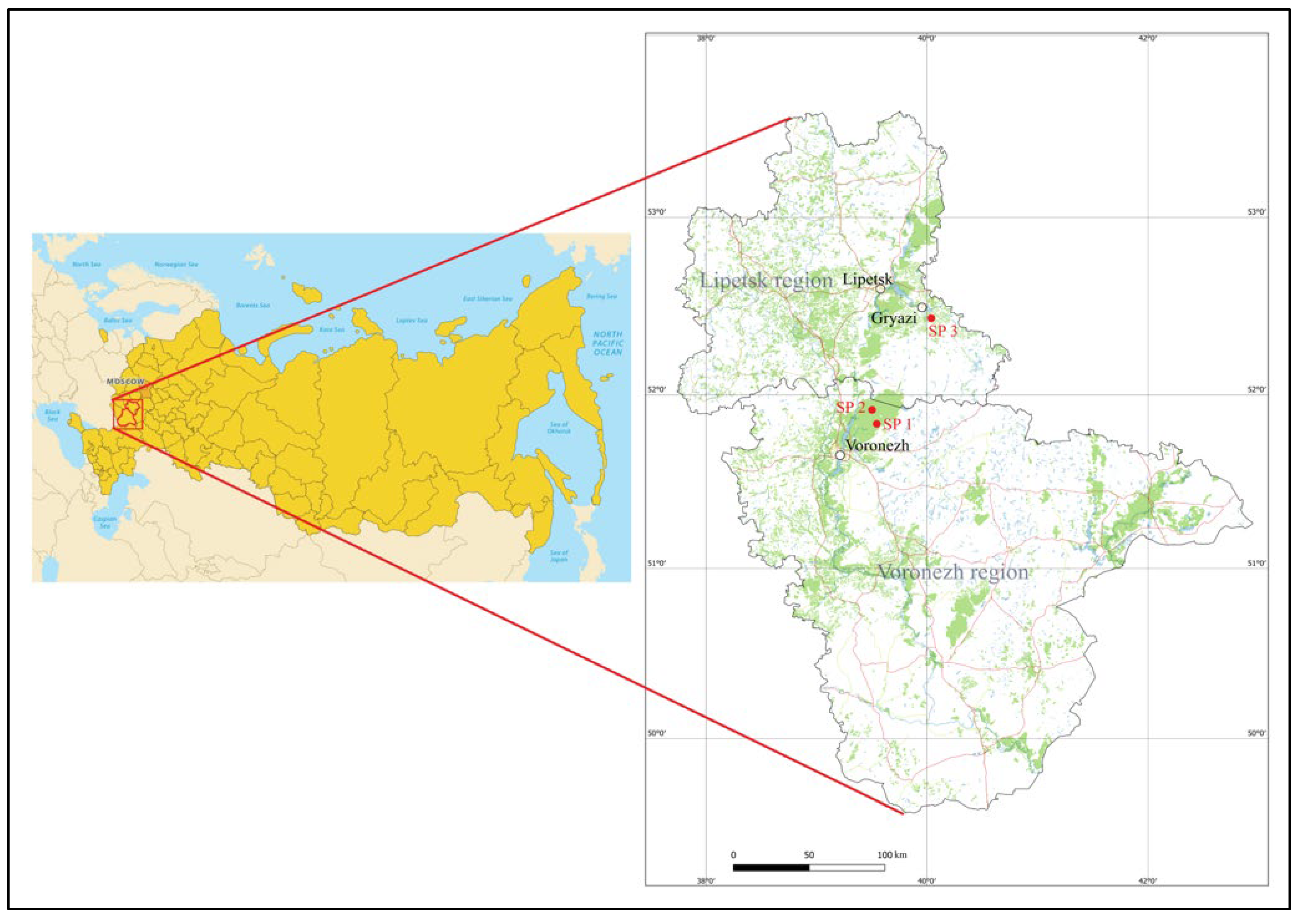
Figure 2.
Histogram of tree height distribution, and Weibull, lognormal, and gamma distributions for sample plots SP1 (a), SP2 (b), and SP3 (c).
Figure 2.
Histogram of tree height distribution, and Weibull, lognormal, and gamma distributions for sample plots SP1 (a), SP2 (b), and SP3 (c).
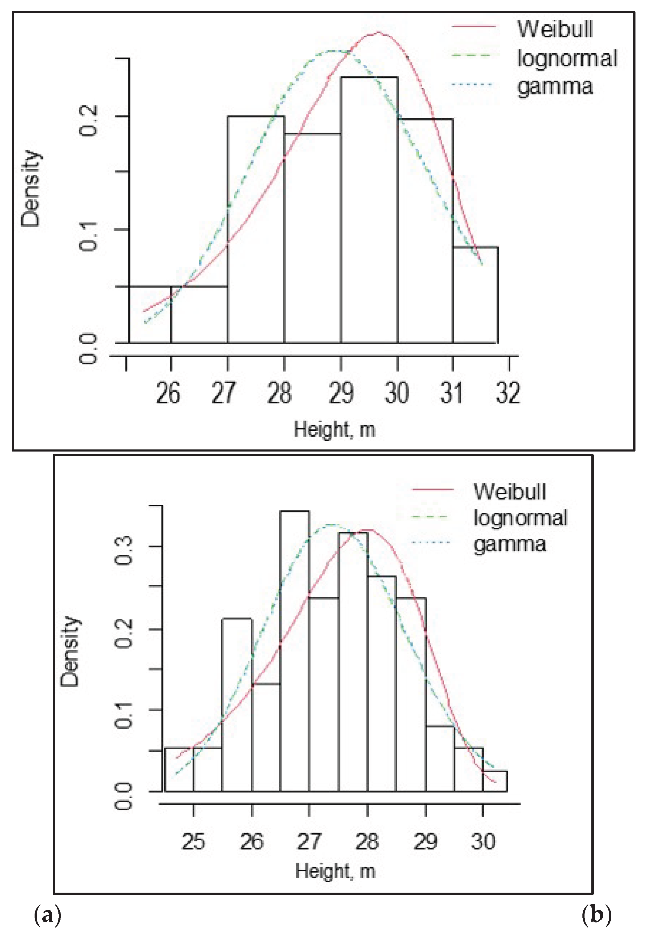
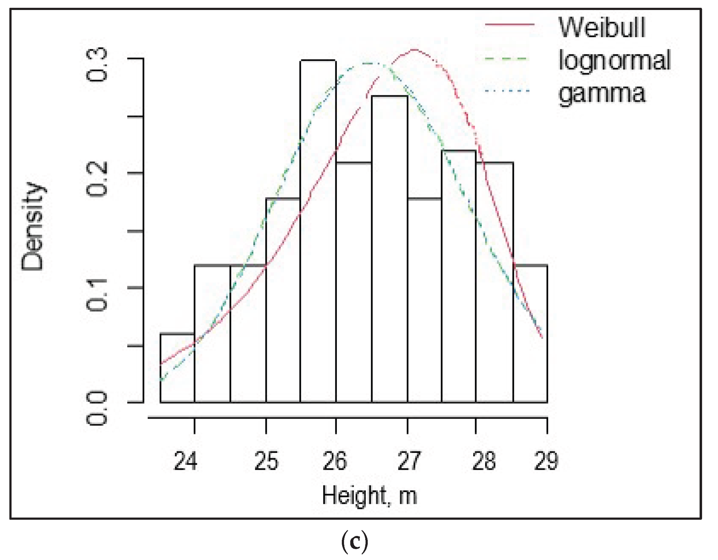
Figure 3.
Histogram of tree diameter distribution, and Weibull, lognormal, and gamma distributions for sample plots SP1 (a), SP2 (b), and SP3 (c).
Figure 3.
Histogram of tree diameter distribution, and Weibull, lognormal, and gamma distributions for sample plots SP1 (a), SP2 (b), and SP3 (c).
Figure 4.
The relationship between trunk diameter and height in sample plots SP1 (a), SP2 (b), and SP3 (c) using the two-parameter nonlinear Näslund model.
Figure 4.
The relationship between trunk diameter and height in sample plots SP1 (a), SP2 (b), and SP3 (c) using the two-parameter nonlinear Näslund model.
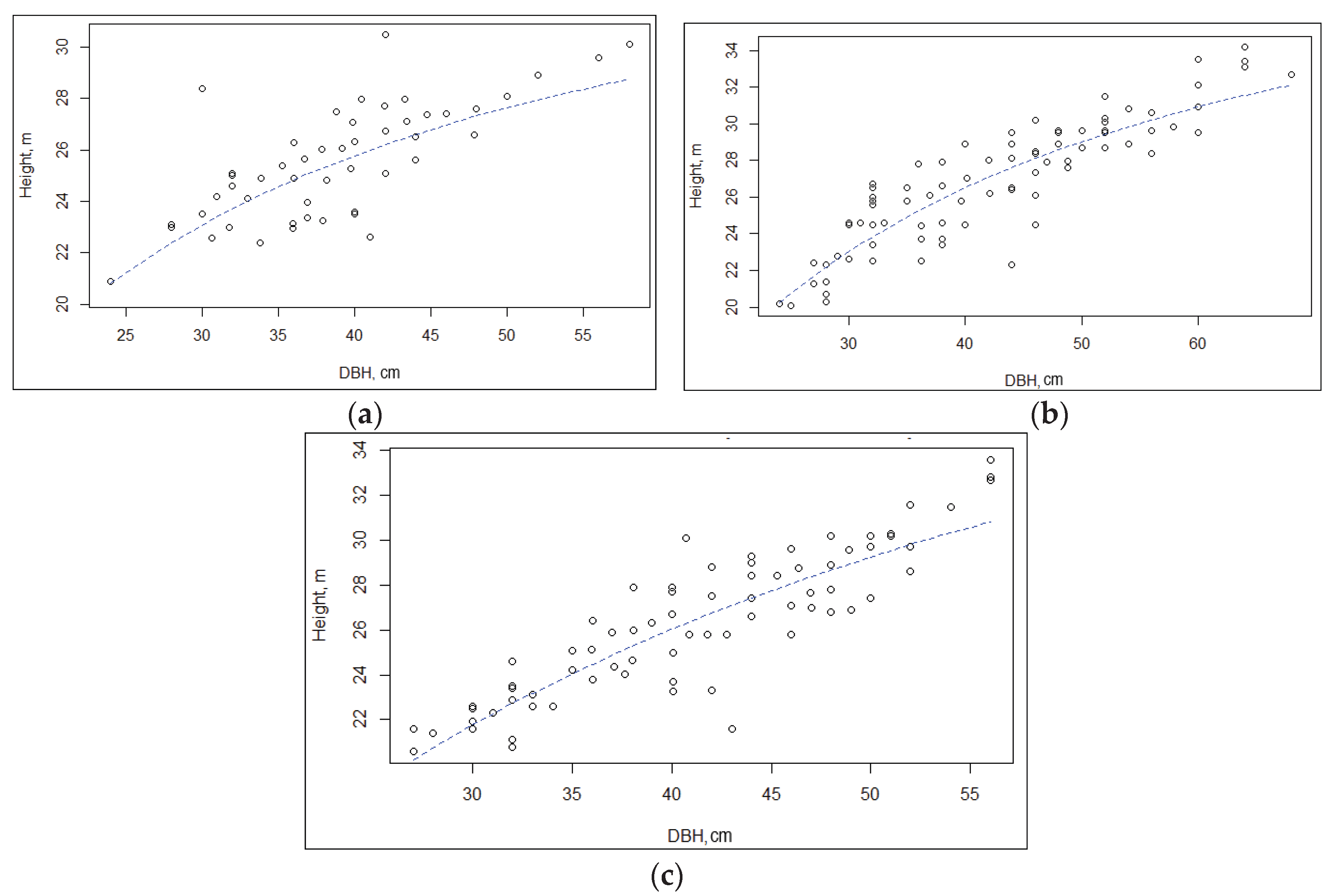

Table 1.
Forest mensuration characteristics of Scots pine stands on the sample plots SP1, SP2, and SP3.
Table 1.
Forest mensuration characteristics of Scots pine stands on the sample plots SP1, SP2, and SP3.
| Sample plot | Size, ha | Tree species composition | Tree age, years | DBH, cm | Height, m | Tree density | Volume stock, m3 ha-1 | Forest site type |
| SP1 | 0.25 | 100% Scots pine | 140 | 42.2 | 28.5 | 0.6 | 450 | moderately moist and moderately fertile soil |
| SP2 | 0.25 | 100% Scots pine + English oak with less than 5% | 130 | 48.5 | 29.0 | 0.7 | 490 | moist and moderately fertile soil |
| SP3 | 0.25 | 100% Scots pine | 120 | 41 | 27.5 | 0.6 | 420 | moderately moist and moderately fertile soil |
Table 2.
Sanitary conditions of Scots pine trees in the sample plots SP1, SP2, and SP3.
| Sample plot | Sanitary category, % of trees | Average weighted condition category | |
| 1st (healthy) | 2nd (weakened) | ||
| SP1 | 65 | 35 | 1.4 |
| SP2 | 90 | 10 | 1.1 |
| SP3 | 50 | 50 | 1.5 |
Table 3.
Underbrush bush species in the sample plots SP1, SP2, and SP3, plants per ha.
| Species | SP1 | SP2 | SP3 |
| Red raspberry (Rubus idaeus L.) | 1120 | 800 | - |
| Red elderberry (Sambucus racemosa L.) | 240 | - | 240 |
| Common rowan (Sorbus aucuparia L.) | 240 | 1120 | - |
| Alder buckthorn (Frangula alnus L.) | - | 240 | 800 |
| Warty spindle (Euonymus verrucosus L.) | - | 600 | 240 |
| Common hazel (Corylus avellana L.) | - | - | 80 |
| Common pear (Pýrus commúnis L) | 80 | - | - |
| Total | 1680 | 2760 | 1360 |
Table 4.
Projective cover (%) of ground cover species on the sample plots SP1, SP2, and SP3.
| Species | SP1 | SP2 | SP3 |
| Lily of the valley (Convallaria majalis L.) | 45 | - | 35 |
| Common haircap moss (Polytrichum commune L.) | 5 | 10 | - |
| Bushgrass (Calamagrostis epigejos Roth.) | 5 | - | - |
| Cow-wheat (Melampýrum pratense L.) | 5 | - | 5 |
| Common Solomon’s seal (Polygonatum multiflorum L.) | 5 | - | - |
| Moneywort or creeping jenny (Lysimachia nummularia L.) | - | 15 | - |
| Bracken (Pterídium aquilínum L.) | - | 30 | - |
| Red-stemmed feathermoss or Schreber’s big red stem moss (Pleurozium schreberi L.) | 10 | - | 20 |
| Round-leaved wintergreen (Pyrola rotundifolia L.) | - | 10 | - |
| Narrow-leaved lungwort or blue cowslip (Pulmanaria angustifolia L.) | 5 | - | - |
| Wild strawberry (Fragaria vesca L.) | 20 | - | 15 |
| Bloody cranesbill or bloodred geranium (Geranium sanguineum L.) | - | - | 5 |
| Yellow bedstraw or Lady’s bedstraw (Galium verum L.) | - | - | 5 |
| Corn speedwell (Veronica arvensis L.) | - | - | 5 |
| Sidebells wintergreen (Orthilia secunda L.) | - | - | 10 |
| Scotch heather or ling (Calluna vulgaris L.) | - | 10 | - |
| Bristly haircap (Polytrichum piliferum L.) | - | 10 | - |
| False lily of the valley or May lily (Maianthemum bifolium L.) | - | 5 | - |
| Pipsissewa or umbellate wintergreen (Chimáphila umbelláta L.) | - | 5 | - |
| Common clubmoss or running clubmoss (Lycopodium clavatum L.) | - | 5 | - |
Table 5.
Projective cover of ground cover by ecological-cenotic groups on the sample plots SP1, SP2, and SP3, %.
Table 5.
Projective cover of ground cover by ecological-cenotic groups on the sample plots SP1, SP2, and SP3, %.
| Ecological-cenotic group | SP1 | SP2 | SP3 |
| Forest | 75 | 67 | 38 |
| Fotest-meadow | - | 11 | 12 |
| Meadow | 25 | 22 | 50 |
Table 6.
Statistical parameters of the tree diameters and heights at the sample plots SP1, SP2, and SP3.
Table 6.
Statistical parameters of the tree diameters and heights at the sample plots SP1, SP2, and SP3.
| Sample plot | Diameter | Height | ||||||
| Average, cm ± s.e. | CV, % | Asymmetry | Kurtosis | Average, m ± s.e. | CV, % | Asymmetry | Kurtosis | |
| SP1 | 42.2 ± 0.1 | 27 | 0.21 | -0.18 | 28.5 ± 0,2 | 15 | -0.13 | -0.42 |
| SP2 | 48.5 ± 0.2 | 36 | -0.45 | 0.45 | 29.0 ± 0,1 | 24 | -0.36 | -0.79 |
| SP3 | 41.0 ± 0.3 | 33 | -0.03 | -0.13 | 27.5 ± 0,1 | 22 | -0.26 | -0.80 |
Table 7.
Statistics of goodness of fit of simple models to experimental data.
| Distribution | Kolmogorov–Smirnov (D) test | χ2-test | RMSE | MAE | MBE | ||
| D | P | χ2 | P | ||||
| SP1 | |||||||
| gamma | 0.135 | 0.002 | 35.5 | 0.004 | 0.044 | 0.037 | 0.024 |
| lognormal | 0.119 | 0.0003 | 28.1 | 0.0005 | 0.053 | 0.042 | 0.033 |
| Weibull | 0.112 | 0.001 | 30.1 | 0.001 | 0.043 | 0.035 | 0.029 |
| SP2 | |||||||
| gamma | 0.124 | 0.001 | 28.1 | 0.0004 | 0.054 | 0.043 | 0.033 |
| lognormal | 0.121 | 0.003 | 29.3 | 0.0006 | 0.055 | 0.041 | 0.035 |
| Weibull | 0.110 | 0.0001 | 26.6 | 0.002 | 0.035 | 0.024 | 0.069 |
| SP3 | |||||||
| gamma | 0.121 | 0.0002 | 26.4 | 0.003 | 0.055 | 0.013 | 0.088 |
| lognormal | 0.103 | 0.003 | 25.5 | 0.0003 | 0.065 | 0.089 | 0.074 |
| Weibull | 0.136 | 0.0005 | 35.5 | 0.0006 | 0.023 | 0.051 | 0.089 |
Table 8.
Correlation (r) of the CV of height with the number of trees per a ha and the tree diameter.
Table 8.
Correlation (r) of the CV of height with the number of trees per a ha and the tree diameter.
| Sample plot | Number of trees per a ha | Tree diameter | ||
| r | P | r | P | |
| SP1 | 0.83 | < 0.05 | -0.80 | < 0.05 |
| SP2 | 0.78 | < 0.05 | -0.75 | < 0.05 |
| SP3 | 0.88 | < 0.05 | -0.82 | < 0.05 |
Table 9.
Näslund equations of the relationship between the height (H) and the trunk diameter (D) at a height of 1.3 m (DBH) for pine trees in the sample plots SP1, SP2, and SP3.
Table 9.
Näslund equations of the relationship between the height (H) and the trunk diameter (D) at a height of 1.3 m (DBH) for pine trees in the sample plots SP1, SP2, and SP3.
| Sample plot | Equation | RMSE | MAPE | MAE | R2 |
| SP1 | H = 1.3+(DBH/(1.460477+0.15601×DBH))2 | 2.24 | 0.15 | 2.49 | 0.93 |
| SP2 | H = 1.3+(DBH/(1.843485+0.153097×DBH))2 | 1.87 | 0.16 | 1.90 | 0.96 |
| SP3 | H = 1.3+(DBH/(2.393178 +0.177398×DBH))2 | 1.63 | 0.21 | 1.65 | 0.92 |
Table 10.
Phytomass reserves (t/ha / %) in the sample plots SP1, SP2, and SP3.
| Sample plot | Needles | Branches | Trunks | Aboveground phytomass | Underground phytomass | Total |
| SP1 | 8.0 / 6.0 | 20.9 / 8.5 | 148.7 / 60.5 | 177.6 / 75.0 | 67.9 / 25.0 | 245.5 / 100 |
| SP2 | 14.2 / 4.0 | 37.1 / 10.0 | 211.9 / 58.0 | 263.2 / 72.0 | 102.6 / 28.0 | 365.8 / 100 |
| SP3 | 8.2 / 7.6 | 20.5 / 8.4 | 135.7 / 58.0 | 182.4 / 74.0 | 62.5 / 26.0 | 244.9 / 100 |
Table 11.
Carbon content (tC/ha) in the pool of aboveground and underground phytomass in the sample plots SP1, SP2, and SP3.
Table 11.
Carbon content (tC/ha) in the pool of aboveground and underground phytomass in the sample plots SP1, SP2, and SP3.
| Sample plot | Needles | Branches | Trunks | Aboveground phytomass | Underground phytomass | Total |
| SP1 | 4.0 | 10.4 | 74.3 | 88.7 | 33.9 | 122.6 |
| SP2 | 7.1 | 18.5 | 105.9 | 131.5 | 51.3 | 182.8 |
| SP3 | 4.1 | 10.2 | 67.3 | 81.6 | 31.3 | 112.9 |
Disclaimer/Publisher’s Note: The statements, opinions and data contained in all publications are solely those of the individual author(s) and contributor(s) and not of MDPI and/or the editor(s). MDPI and/or the editor(s) disclaim responsibility for any injury to people or property resulting from any ideas, methods, instructions or products referred to in the content. |
© 2025 by the authors. Licensee MDPI, Basel, Switzerland. This article is an open access article distributed under the terms and conditions of the Creative Commons Attribution (CC BY) license (http://creativecommons.org/licenses/by/4.0/).
Copyright: This open access article is published under a Creative Commons CC BY 4.0 license, which permit the free download, distribution, and reuse, provided that the author and preprint are cited in any reuse.


