
Submitted:
31 January 2025
Posted:
03 February 2025
You are already at the latest version
Abstract
This study looked at the impact of planting year differences on vegetation and soil parameters in Pinus sylvestris plantation forests in northern Mongolia. Tujiin nars region has three study sites: 18- to 20-year-old plantation forests planted in 2003, 2004, and 2005, as well as natural regeneration stand, natural forest, and steppe area. Three plots with distinct plantation stand types were constructed at each location to investigate changes in vegetation and soil attributes. Species richness, total coverage, and biomass accumulation were significantly higher in the oldest plantation (2003). This is consistent with the results, where BBS (2003 plantation) had the highest species richness (32 species), plant coverage (58.5%), and above-ground biomass (1159.6 g m2). Soil pH across plantations, with steppe and forest edge soils being alkaline and plantation soils slightly acidic. This matches the results, where soil pH ranged from 6.52 to 7.41, with plantations being slightly acidic. Available nitrogen (3.16 mg kg-1), soil organic carbon (10.1 g kg-1), and carbon stock (9.16 Mg ha-1) were higher in top soil and decreased by depth of profile and differed in plantations by year-of-planting. Furthermore, the change in understory vegetation was significantly correlated with soil moisture, fertility, and species composition was driven by over story density and crown parameters.
Keywords:
Pinus sylvestris
; plantation
; understory vegetation
; forest steppe
; soil properties
; natural regeneration
1. Introduction
Mongolia is a low-forest cover country of 7.9% and only 67.5% of this is closed forest. Pinus sylvestris L is one of the most economically important timber species even though the distribution is limited in Mongolia to the sub-taiga zone [1]. The southern border of P. sylvestris distribution dips into northern Mongolia with the main areas in the Khentii mountain range, along the ridge of Khantai-Buren-Buteeliin in the northwest to Orkhon-Selenge catchment, and the south in the Onon-Balj-Barkhiin river basins, and to the northeast along Bayan-Uul-Ereen davaa area [2]. Reforestation activity in Mongolia started in the 1970s and resulted in a National Forest Policy that considered reforestation and tree planting as key objectives. Restoration and reforestation activities encounter numerous challenges caused by both biotic and abiotic factors. Soil moisture is one of Mongolia's most limiting environmental factors for tree growth and survival. Thus, the selection of appropriate seed sources that have advanced drought tolerance and growth performances could be the best option to promote the quality of planting stocks, obtain high survival of seedlings, and increase growth and productivity in large-scale rehabilitation and reforestation. This unique pine forest ecosystem plays an important role in environmental sustainability including biodiversity conservation, soil protection from erosion, wildlife habitat, and carbon sequestration [3]. The restoration project of the Scots pine forest of Tujiin nars was implemented between 2003 and 2005 with the financial support of the Yuhan Kimberly (YK) company as an example of forest restoration and afforestation in the forest-steppe region of Mongolia. Over the last two decades, more than 21,000 ha of Scots pine plantations were established on clear-cuts and burnt forest areas using native tree species in the region [4]. The success of planting and reforestation depends upon many factors, including seed and seedling quality, site-species compatibility, and appropriate silvicultural practices [5].
Therefore, plantation forest need often maintenance such as a thinning, which is significantly influences forest soil, affecting root density, microbial communities, organic matter turnover, and nutrient budgets, which affects tree growth, understory vegetation composition, and the whole forest ecosystem [6,7,8]. Tree planting can change soil environments by affecting soil temperature and moisture, bulk density, and soil organic carbon [9,10,11,12]. We evaluated the understory vegetation and soil parameters associated with 18 to 20-year-old plantation forests that were in 2016 and 2017 to offer answers to this topic. (1) to assess the environmental consequences of new forests on understory vegetation; and (2) to access the changes of soil characteristics under plantation forests. Our findings will aid efforts to enhance the management of current plantations and urge planners to employ Scots pine only at the most appropriate densities and locations in future afforestation.
2. Materials and Methods
2.1. Study Area and Site Description
This study area is located in the territory of Tujiin nars Nature Conservation Park, which administratively belongs to Selenge province (50005’ and 50012’N, 106014’ and 106031’E) in northern Mongolia with an elevation ranging between from 650 to 750 m asl (Figure 1). The park stretches approximately 33 km from east to west and covers an area of 73,000 ha, of which 45,800 ha are natural pine forests and 21,000 ha are Scots pine plantations [4]. Tujiin nars lies within the northern temperate and boreal forest that is distributed along the southern edge of the Siberian Taiga, at the forest-steppe transitional zone called sub-taiga forests [[17]. According to the updated world map of the Kӧppen–Geiger climate classification [18], the region lies within the transition climatic zone between a cool continental climate (Dwc) and a cold semi-arid climate (Bsk), with small pockets exhibiting a temperate continental climate (Dwb). The main tree species in this forest include Siberian larch (Larix sibirica Ldb.), Scots pine (Pinus sylvestris L.), Siberian pine (Pinus sibirica Du Tour.), Asian white birch (Betula platyphylla Sukaczev.), and European aspen (Populus tremula L.) [19].
The mean annual temperature was 0.6±0.0020C and mean annual precipitation was 280.3±7.3 mm with a precipitation peak between June and August (Figure 2) according to the nearest meteorological station located at Sukhbaatar (N 50014’35.063”; E 106010’23.008”, 621 asl). The soils in the study site are Arenic podzols (also called Derno-Forest soils in Mongolia), which were derived from sandy sediments and loess. The sandy loess stratum, which provides the parent materials, is extremely thick and is widely distributed in the study region. The soil is characterized by relatively good water retention but is poorly vegetated due to climate [20].
2.2. Measurements and Sampling Design
2.2.1. Sampling Design
Sample plots for comparative growth analyses were established in three Scots pine plantations, and each plot had been four replicates. One additional sample plot was established in a naturally regenerated young stand for a total of 6 plots. Each 20 m x 20 m (400 m2) sized sample plot was established in a representative part of each treatment. The geographical location and site description of the sample plots is illustrated in Table 1.
2.2.2. Vegetation Survey
Investigation of herbal plant cover and species diversity was carried out in 6 sample plots established in the forest plantations, a naturally regenerated young stand, and at the forest edge and steppe area (Table 1). Vegetation was surveyed in 1 m2 quadrat sample plots at the center and each of the opposite corners of the sample plots. Clearly mark off a 1 m² square using stakes, string, or any other method to delineate the area. Identify all plant species within the plot. For this method, you're interested in the foliar cover—the amount of the plot covered by the leaves or above-ground parts of the plants. For each species present in the plot, estimate its abundance and coverage based on visual estimates. The Braun-Blanquet method uses a cover-abundance scale, which is a set of categories that describe the proportion of the area covered by each species [21]. Species presence, number, and coverage data was used to estimate species richness and vegetative cover. The species richness defined as the number of species per plot [22]. Vegetation cover was estimated as the ratio of the vertical projection of exposed leaf area to the area of each quadrat.
Importance value, species diversity indices and similarity indices were calculated to compare vegetation change in the sample plots [23]. Importance value (IV) was calculated with relative frequency and relative coverage to identify indicator species [24]. Difference in species diversity assessed by species richness, the Shannon-Weiner index [25], and an evenness index (J) was calculated as the ratio of observed density (H') to maximum density (Hmax) [26]. Simpson’s index (D) was calculated to measure community diversity [27]. Bray and Curtis (BC) [28] and Sorensen (SS) [29] indices of similarity were calculated for all pairs of plots, including naturally regenerated stand, plantation forest, forest edge, and steppe [30].
After vegetation survey, all individuals were harvested (including roots) in each quadrat and weighed to obtain fresh weight. Above- and below-ground components were separated and oven-dried at 800C for 72 hours to estimate dry biomass. The nomenclature of the species followed the Conspectus of the Vascular Plants of Mongolia [31], which was based on the APG III [32] of plant classification. Collected materials were identified based on the Key to the Vascular Plants of Mongolia [33,34]. Families and species were listed in accordance with APG IV [35]. The ecological groups of plants by [36] and the information on the conservation status was based on the International Union for Conservation of Nature (IUCN) Red List, Urgamal et al. [31], Nyambayar et al. [37], the Red Data Book of Mongolia [38], and the Appendix to the Mongolian Law of Natural Plants [39].
2.2.3. Soil Survey
Soil sampling was conducted relative to the two soil sampling plots at each site. Representative 20 x 20 cm subplots were excavated to a depth of 100 cm. Morphological characteristics were recorded and soil samples taken from the horizons of the excavated profiles at 0-5 cm, 5-10 cm, and at 10 cm intervals from 10 to 100 cm (total of 122 samples). Undisturbed soil cores were taken from the upper part of each horizon to determine bulk density (BD) and soil moisture (in total 198 samples), using 5-cm-tall metal cylinders, 95 cm3 in volume. Soil temperature was measured at each depth of the soil profile with an accuracy of ±0.2°C. The soil temperature readings were conducted on July 24–25, 2020, between 12:00 PM and 4:00 PM, during the peak summer temperature period. The measurements were punctual and taken at each depth of the soil profile with three repetitions using the Digital Thermometer HI98501 Checktemp (Hanna Instruments Inc.), which has an accuracy of ±0.2°C. A total of 33 soil temperature data points were collected for each soil profile.
Soil samples were air dried, sieved through a 2 mm sieve and stored at room temperature. The samples were subjected to the following physical and chemical analyses [40]. Particle size was determined by pipette [41]; pH was determined on a 1:2.5 air-dried soil/distilled water mixture using a glass electrode pH meter [42]. Electrical conductivity (EC) was determined for a 1:5 air-dried soil/distilled water mixture using a platinum electrode. Soil organic carbon was measured by the Walkley and Black [43] method and organic carbon stock was determined according to Batjes [44]. Calcium carbonate content was determined by the volumetric method [45]. Available phosphorus (P2O5) was measured by molybdenum blue colorimetry, after (NH4)2CO3 digestion [46]. Nitrate-nitrogen (NO2-N) determined using a CH3COONa digestion and spectrocolorimetry. Potassium (K2O) was analyzed by flame spectrometry [47].
2.3. Statistical Analysis
The SAS software package, version 9.4 [48] was used for statistical analysis. A one-way analysis of variance (ANOVA) was adopted to assess the significance of differences among stands, year of planting (YoP) on the stand characteristics, vegetation (species richness, coverage), as well as soil properties (moisture content, pH, soil organic carbon). Duncan’s multiple range test (DMRT) was used for multiple comparisons among the 2020 data.
Correlation between above-ground and below-ground understory biomass of different plots and regression analysis between climatic characteristics and diameter increment was carried out using the statistical program SPSS [49]. Numerous visualizations of PCA scatter plots and heat maps illustrate the relationships between variables (soil characteristics and understory vegetation values by plots) in the dataset, while integrating statistical methods through the ggplot2, pheatmap, complexheatmap, and tidyverse packages in the R programming language [50].
3. Results
3.1. Understory Vegetation Composition and Their Change
Understory vegetation was comprised of 92 species of plants, including 4 shrubs, 1 semi-shrub, species and 84 herb species (5 annuals and 87 perennials) belonging to 78 genera of 35 families. The dominant families were Asteraceae (15 species, 16.3%), Rosaceae (10 species, 10.8%), Ranunculaceae, Poaceae, Fabaceae (each with 7 species, 7.6%) and followed by Lamiaceae (4 species, 4.3%), Iridaceae (3 species, 3.3%) and Caryophyllaceae (3 species, 3.3%). Dominant species were mesophytes (36 species, 39.1%), xerophytes (30 species, 32.6%), petrophytes (4.35%), and gigrophytes (1.08%). Mesophyte species dominated in the plantations (BBS 50%, MGS 56.7%, BDS 52%) and the naturally regenerated stand (NRS 52%); xerophytes were greater in the natural forest edge (NFM 52.6%) and the steppe (STP 46.9%) plots (TableS1).
Species richness was significantly different between the six plots (p=0.0352), with higher total values registered in BBS (32 species) and the lowest total richness and cover detected in NRS (8 species). Total plant coverage was significantly different (p=0.0001); BBS had the greatest (58.5%) and MGS had the lowest (26.5%) cover (Figure 3).
Above-ground (AGB) and below-ground (BGB) biomass accumulation was highest in BBS (AGB = 1159.6 g m-2, BGB = 3325 g m-2). The lowest Above-ground biomass was observed at NRS (AGB = 44.0 g m-2) and the lowest below-ground biomass was observed in BDS (BGB=137.0 g m-2) (Figure 4).
There were few significant correlations between stand characteristics and species richness, plant coverage and above- and below-ground biomass (Table 2). Tree crown length and tree height were positively correlated with above- and below-ground biomass but negatively correlated with crown projection area. Correlations between soil pH and bulk density understory biomass were negative (Table 3). Soil moisture was positively correlated with plant cover in the naturally regenerated (NRS) plot, species richness in the near forest (NFM) plot, and above-ground biomass in the steppe plots (STP). Plant coverage was negatively correlated with soil pH, bulk density and soil moisture at the NRS plot. Soil organic carbon was positively correlated with above-ground biomass in the steppe plot.
Importance value were used to describe and compare the species dominance, with highest IV index considered to be most “important” in a specific plot. Agrimonia pilosa, Festuca valesiaca, Linum sibiricum species were had high IV values and dominated in 2003 plantation named a BBS plot. Phlomis tuberosa and Sibbaldia adpressa species were dominated in 2004 plantation, NGS. Theremore, Cleistogenes squarrosa, Cirsium esculentum, and Elymus sibirica species were dominated and had high IV in 2005 plantation, BDS (Table 4).
But in naturally regenerated and natural plots IV values and dominated species were little bit different. Elymus sibiricus, Phlomis tuberosa species were had high IV values and dominated in natural regenerated stand (NRC). Allium bidentatum, Carum carvi, Fragaria orientalis and Phlomis tuberosa species were dominated in natural forest edge (NFM), but Cleistogenes squarrosa, Festuca valesiaca, Patrinia rupestris, Linum sibiricum, Allium linare and Caragana microphylla species were dominated and had high IV in Steppe area, STP (Table 5).
There were significant differences among plots in diversity index (H’), evenness index (J), and Simpson index (D) as shown in Table 6. The diversity Shannon index in BBS has the highest value (0.8156), indicating the most diverse plot, MGS has the lowest value (0.172), showing the least diversity. The Evenness Index MGS has the highest evenness (0.4966), suggesting a more balanced species distribution. NFM has the lowest evenness (0.0869), indicating dominance by a few species. The Simpson Index is BBS has the highest value (1.1638), showing the least dominance and highest diversity. NRS has the lowest value (0.0855), indicating high dominance by a few species. As the result BBS is the most diverse plot across all indices. MGS has high evenness but low diversity, suggesting fewer species distributed evenly. NRS shows high dominance, with a few species dominating the plot BBS-1 was significantly higher that other plots, while the lowest was MGS-1; on the contrary, MGS had the highest evenness index and the lowest was NFM (Table 6).
The table presents similarity coefficients (Bray-Curtis and Sorensen) for two plot groups, assessing ecological similarity based on species composition. Bray-Curtis (BC) dissimilarity Coefficient: Assesses the dissimilarity between two groups (values approaching 0 signify greater similarity). BBS, MGS, BDS, NRS: 0.30 (moderate dissimilarity). STP and NFM: 0.28 (marginally more analogous than the initial group). Sorensen (Ss) Coefficient: Assesses similarity as a percentage, with larger values signifying increased similarity. BBS, MGS, BDS, NRS: 20.83% (little resemblance). STP and NFM: 46.81% (moderate resemblance, surpassing the initial group). STP and NFM have greater ecological similarity to one another than to the group comprising "BBS, MGS, BDS, NRS". The Bray-Curtis values correspond with the Sorensen percentages, indicating that the second group exhibits greater similarity (Table 7).
3.2. Soil Chemical and Physical Properties and Their Change
Regarding the soil classifications, gradient, and altitude of various plots. We analyzed the disparity among plots utilizing the Kruskal-Wallis test in the R programming language. The Kruskal-Wallis rank sum test revealed a chi-squared value of 5, with 5 degrees of freedom and a p-value of 0.4159, indicating no statistically significant differences across plots concerning either elevation (p = 0.4159) or slope (p = 0.4159). Physical and chemical properties of the soils (0-100 cm) and by depth are presented in Table 8, Table 9 and Table 10 indicate significant differences both among sample plots and soil depths. Soil pH varied between 6.52-7.41; plantation forests had slightly acidic soils grading into slightly alkaline soils at the natural forest edge and steppe. The difference in soil pH in the 2003 plantation was not significant, and the mean soil pH was lower than that in other plots. Nevertheless, bulk soil pH (from 0-30 cm depth) tended to be similar in all plots (Table 8).
Available nitrogen was highest in STP plot (3.64±0.34 mg kg-1) and lowest in BBS plot (BBS; 1.79±0.13 mg kg-1). Carbonate (CaCO3) was observed in the soils of the forest edge (NFM) and steppe (STP) at the depth of 90 cm and 30 cm, respectively. The available nitrogen content, organic carbon and carbon stock of plantation forests differed according to their year-of-planting, with BBS<MGS<BDS. The measured soil properties significantly differed by depth (0-30 cm; 30-60; 60-100 cm) except for available phosphorus content (Table 8). Available nitrogen (3.16 mg kg-1), soil organic carbon (10.1 g kg-1), carbon stock (9.16 Mg ha-1) and available potassium (114.6 mg kg-1) were higher in the top soil (0-30 cm) and decreased by depth of the soil profile (Table 8).
The mean values of soil bulk density in the 0-100 cm soil depth varied from 1.42 to 1.54 g cm-3 (Table 8); BDS had the highest value (p=0.0001) but there were no significant difference plots (p=0.5657). All the soils were generally sandy, with a high proportion of sand (89.3%) and a low proportion of fine particles (clay 9.3% and silt 11.4%) and similarly the top soil (0-30 cm) has higher proportion of sand (79.2%) than in 30-60 cm (9.3%) and 60-100 cm (11.5%) depths. The sand fraction was dominant in the top soil (0-30 cm); content varied from 63% to 83%. Smaller amounts of silt (from 8.42-19.75%) and clay (8.6-17.0%) were present and there were statistically significant differences in texture among the selected study areas.
3.2.1. Changes in Chemical and Physical Properties of the Top Soil
The soil pH significantly differed in the topsoil of the plots, with a lower pH in the soils of the BBS (6.10) than in soils of the other plots (Table 9) and top soil pH of 2005 plantation (BDS) was 7.39, which were higher than in soils of the STP plot (7.00). Similarity of pH values between BBS and NRS plots indicates that soil pH in plantation forest is getting similar to naturally regenerated forests, but on the other hand, similarity between BDS (2005 plantation) and STP shows slow recovery after disturbance. However, Soil other chemical properties are not significantly the soil temperature significantly differed in the topsoil. Soil temperature varied between 17.7-24.70C, where the lowest temperature was in the naturally regenerated stand and highest was in the steppe plot, and generally air temperature in plantation forests was lower than in the steppe and at the forest edge (Table 9). The soil temperature of BBS stands and 2.30C higher than in the naturally regenerated stand (NRS). The average soil moisture of soils in different sample plots varied from STP (5.1%) to MGS (12.0%) and decreased soil moisture by 2.0% in the 2003 plantation forest. Soil bulk density was significantly different among the plots with lower values in BBS and NRS (1.23-1.25 g cm-3) than other plots. Bulk density of the 2005 plantation and steppe plots were similar, averaging 1.46 g cm-3.
3.2.2. Changes in Chemical and Physical Properties of the Subsoil
There were statistically significant differences in the organic carbon content (p<0.01) and carbon stock (p<0.01) between the plots and lower content in steppe plots (STP). Even so, no significant differences were observed (p=0.548) among plots in soil organic carbon and carbon stock, although there was a slight decrease in organic carbon stock (Table 9). Mean values of soil organic carbon and carbon stock of plantation forests (5.93 g kg-1; 9.08 Mg ha-1) were higher than that of steppe (2.19 g kg-1; 3.31 Mg ha-1). The highest organic carbon (9.97 g kg-1), available phosphorus (39.19 mg kg-1) and potassium (103.0 mg kg-1) were recorded in the soil of the BBS plot. The lowest contents of carbon (2.19 g kg-1) and available phosphorus (14.03 mg kg-1) were found in the soil of the STP plots, MGS, with the lowest available potassium content in the MGS and BDS plots (Table 10). Also, there were statistically significant differences in the soil pH (p<0.001) and soil temperature (p<0.001) between the plots, with a lower pH in the soils of the BBS (6.10) than in soils of the other plots. Soil pH of the subsoil was same situation like soil pH in the top soil.
There were statistically significant differences in the soil clay (p<0.001), soil temperature (p<0.001) between the plots, with a higher clay in the soils of the BBS and NRS (15.1; 13.9%) than in soils of the other plots (Table 10). The soil temperature of NFM, STP stand and 4.10C higher than in the naturally regenerated stand (NRS), BBS, MGS. BBS.
3.2.3. Statistical Analysis of the Understory Vegetation Composition and Soil Chemical and Physical Properties Between Different Plantation Plots
According to our PCA analysis, it was particularly evident that variation in soil chemical and physical characteristics are positively different in the BBS, MGS, NFM are than other plots, but in particular, understory vegetation data shows STP and BDS are more different from other plots (PCA 1 33.2%, PCA 2 18.2%) (Figure 5a). Moreover, when we used the heatmap approach, we obtained a clear indication that in all plots. From this, BBS and MGS plots' vegetation characteristics are higher without species richness. But soil characteristics are BBS and BDS plots; SOM, EC, AP, AK Clay, and SM are higher, but STP and NFM plots are shown as the lowest in all soil characteristics (Figure 5b, c). Figure 5a) scatter plot illustrates a positive linear correlation between the Shannon Index (H') and pH. The R² value of 0.27 signifies that 27% of the variation in the Shannon Index is elucidated by pH. The dark area surrounding the trend line denotes the 95% confidence interval. The intervals expand near the extremes of pH, signifying more uncertainty in predictions for extremely high or low pH levels. Although the association is positive, the p-value (0.289) indicates that the correlation lacks statistical significance, perhaps due to the limited sample size (n=6). The trend line indicates that for each unit increase in pH, the Shannon Index rises by roughly 0.26 units, as shown by the regression slope. As pH rises from 6.8 to 8.2, the Shannon Index correspondingly increases, signifying that mildly alkaline soils (elevated pH) foster enhanced species diversity.
We also analyzed some soil variables in relation to understory vegetation diversity, as represented in a PCA-derived scatter plot in Figure 6. Shannon Index versus pH: the graph indicates a positive association (R² = 0.27). BBS exhibits the maximum diversity (0.82) at pH 8.2, while BDS demonstrates the lowest diversity (0.26) at pH 6.8. The linear relationship implies that diversity grows by 0.26 units for each unit rise in pH. Confidence intervals expand at pH extremes, signifying increased uncertainty. Slightly alkaline environments (pH 7.5-8.2) seem to promote greater species diversity (Figure 6a). Shannon Index versus Soil Organic Matter (SOM): indicates a positive correlation trend (R² = 0.22). BBS exhibits the highest diversity with the highest SOM (35%), while BDS has the lowest diversity with the lowest SOM (15%). Each 1% increment in SOM is associated with a 0.016 rise in the Shannon Index. Increased organic matter content enhances species diversity, likely due to enhanced soil structure and nutrient accessibility (Figure 6b). Shannon Index versus Electrical Conductivity (EC): demonstrating a tendency of positive association (R² = 0.24). BBS exhibits the maximum diversity at EC 0.8, while BDS displays the lowest diversity at EC 0.3. The linear connection suggests that diversity grows by 0.62 units for each unit increase in EC. Moderate electrical conductivity levels seem advantageous for species variety, potentially signifying appropriate food availability (Figure 6c). All three soil factors (pH, SOM, EC) exhibit positive associations with species diversity. BBS consistently exhibits the greatest values across all metrics, while BDS consistently displays the lowest values. Other plots (MGS, NRS, NFM, STP) typically aggregate within intermediate ranges. Moderate R² values (0.22-0.27) indicate that soil factors account for around 22-27% of the variation in diversity. Additional unquantified variables are expected to affect diversity. The robust interconnection among soil metrics indicates comprehensive soil quality impacts. Improved soil conditions (elevated pH, soil organic matter, electrical conductivity) typically foster greater biodiversity (Figure 6).
4. Discussion
The establishment of productive forest plantations is becoming an important silvicultural issue in Mongolia. In the study region, plantations are primarily monocultures, consisting only of Scots pine (P. sylvestris L.). Scots pine is a light-demanding tree species that plays an important role not only in domestic wood industry, but also in forest ecosystem sustainability in Mongolia. Several open questions regarding Scots pine in Mongolia include whether to plant or rely on natural regeneration; which regeneration method produces the greatest understory diversity; the optimal spacing for planting; and the effect of planting tree on the growth and development of the over story pine, understory diversity, and soil properties?
Soil water content decreased with increasing tree age, while the thickness of the surface dry layer increased, significantly leading to greater soil drying. In the 4-year-old forests, soil moisture was adequate, and seasonal rainfall could partially compensate for the soil water deficit. However, in 9-year-old forests, water deficit became a serious concern at high tree densities, where seasonal rainfall did not compensate completely offset the soil water deficit at densities greater than 400 trees per hectare (trees ha−1). Consequently, the soil remained relatively dry at the end of the rainy season, even after more than 640 mm of rainfall. The 15- and 30-year-old forests also experienced significant drought due to their drying effect on the soil. Overall, the trees promoted soil water loss, creating a serious imbalance between the water supply and demand in this desert environment. High-density planting accelerated the deterioration of the water environment (i.e., soil drying) and threatened the future survival of the trees and other plants. Thus, ecological managers must reduce tree planting and test the effectiveness of reducing the density to 333 trees ha−1 during the young stage [51]. Natural regeneration in the Tujiin nars Scots pine forests has been impeded by fires and grazing, increasing the emphasis on planting to regenerate these forests. Although this study was not designed to directly compare planting with natural regeneration; we included comparisons of the planted stands to a naturally regenerated stand of approximately the same age to highlight different management effect. On one hand, several studies [52,53,54,55] have noted the importance of establishing forest plantations with native tree species, which can have highly diverse understory of indigenous species. On the other hand, Hanter [56] and Hartley [57] stated that plantation forests typically are less favorable as habitat than naturally regenerated stands for a wide range of taxa, particularly in the case in the even-aged, single-species stands. In our case, species richness (30.57-75.18%) and plant coverage (18.4-48.3%) were higher in planted forests than in the naturally regenerated stand (SR-68.16% and PC-48.3%) (Figure 3). The contrary effects may be due to legacy effects of previous land use [58,59]. For example, Hedman et al. [60] found that understory diversity was greater in pine plantations established after harvesting a forest than on old agricultural fields.
Optimal spacing at planting and during subsequent tending must balance several sometimes-competing factors. Stock ability, a concept of optimal growing space [61], depends upon species traits and site quality. Additionally, Optimal planting density must consider competing vegetation to ensure that site resources are captured by the target planted species. Managing stand density at lower levels has been proposed as an adaptation to climate change driven increases in aridity, which is an important consideration in Mongolia [52,63].
Greater diversity and unique composition in the treatments compared to undisturbed control suggested a link between resource heterogeneity and biodiversity [65] or legacy effects associated with different treatments changes in understory plant community, which was partly supported by our study. The Shannon index was highly variable among treatments (Table 7) and generally indicated low species richness, which did not exceed 0.8156 in the BBS.
Open conditions after the removal of previous stands provided an opportunity for non-forest understory species to establish. Changes in species composition and a stable existence of invasive plant species from different ecological groups tend to persist during the initial stage of forest plantation establishment [66]. Mesophytes and xerophytes were the dominant life forms, which are well adopted to dry climatic conditions and relatively infertile soils. Furthermore, the abundant herbaceous species with high plant coverage from steppe and forest-meadow ecological groups were found not only in STP and NFM, but also in other stands. This high proportion of herbaceous species adapted to steppe and forest-meadow ecosystem within planted forests, and their stable existence in the plantations; indicated a potential risk of replacing the Scots pine ecosystem with steppe ecosystems. As tree crown in size over time, they create shade and more suitable microclimatic conditions for the development of forest and forest-meadow plant. Thus, comparisons of understory composition and biodiversity in plantations with other types of forests heavily depend on plantation age.
Forest management significantly affects forest soils, particular soil organic matter, a key component of sustainability [67,68]. Soil is a crucial component in ecosystems, serving as a major storage and source of plant-available nutrients [8]. Change in the soil properties in our study mainly occurred in the topsoil layers (0 to 20 cm). Significant increases in soil bulk density (1.25±0.11 to 1.46±0.06 g cm-3), organic carbon (8.85±2.55 to 15.45±4.32 g kg-1), soil organic carbon stock (8.87±1.34 to 13.39±2.98 Mg ha-1), available phosphorus (21.17±5.02 to 26.42±5.38 mg kg-1) and soil moisture (8.6±1.0 to 12.0±2.5%) were observed in plantations compared to NRS and NFM. The results of the assessments showed a slight increase in soil temperature throughout the soil profile and a sharp decrease in the moisture content of the upper soil layer in 2003 plantations.
Restoration objectives include maintaining pH levels between 7.5 and 8.2, enhancing soil organic matter to 30-35%, sustaining electrical conductivity around 0.7-0.8, and demonstrating potential for improvement in all parameters through biological diversity strategies. Additional plots may gain from specific soil enrichment. Furthermore, we propose that a larger sample size be utilized to enhance statistical significance, alongside temporal monitoring to evaluate seasonal fluctuations, examination of additional environmental factors, and a comprehensive analysis of species composition. Future research directions include long-term monitoring of soil-diversity relationships, investigation of species-specific responses to soil conditions, analysis of soil microbial communities, assessment of restoration success using these parameters as indicators, and examination of climate change effects on soil-diversity relationships.
The results indicate that interventions to elevate soil pH, like as liming, in acidic plots like BDS may promote species diversity. Plots with intermediate pH (e.g., NRS, NFM) may require supplementary soil amendments to enhance conditions for biodiversity. Integrate additional soil variables (e.g., soil organic matter, electrical conductivity) into the analysis to enhance comprehension of their collective impact on diversity. Observe alterations in soil characteristics and biodiversity across time to document temporal dynamics. Responses Specific to Species: Examine the responses of specific species to pH and other soil characteristics to determine the primary factors influencing diversity. Soil organic carbon (SOC) levels in plantation forests are higher compared to grasslands and naturally regenerated forests. In low-carbon soils, forest restoration accumulates significantly more carbon than natural regeneration [70].
Carbon stocks generally decrease with soil depth, as SOC concentrations below 30 cm are less influenced by management practices due to lower carbon inputs and higher decomposition rates in deeper layers. Near the soil surface, SOC concentrations increase non-linearly, driven by carbon inputs from plant residues, roots, and favorable conditions such as optimal temperature and moisture [71]. Maintaining optimal soil moisture levels is crucial for enhancing carbon sequestration and reducing greenhouse gas emissions [72].
Drought conditions, which reduce soil moisture, have a significant negative impact on carbon sequestration. Conversely, in some regions, high soil moisture levels promote carbon accumulation. For example, elevated soil moisture in areas like the Qinghai-Tibetan Plateau, Xinjiang, and Northwest China enhances carbon sink activity, contributing to net ecosystem productivity increases of up to 3.0 g C m² per year [73]. These findings collectively emphasize the strong connection between soil moisture and SOC dynamics. The results from previous studies align with our findings, which establish a clear relationship between soil moisture levels and carbon dynamics, highlighting the importance of soil moisture in SOC accumulation and loss.
The correlation between soil organic carbon (SOC) in forest plots and carbon sequestration trends demonstrates that SOC functions as a crucial reservoir for atmospheric carbon, especially in tropical wet and moist forest ecosystems [74]. The density and diversity of trees in these forest plots positively correlate with soil carbon levels, indicating that healthier and more diversified forests can improve carbon sequestration [75]. Our findings indicate that plantation stands (BBS, MGS, BDS) typically exhibit elevated SOC levels in comparison to natural regeneration stands (NRS) and steppe regions (STP). The detailed BBS exhibits the highest soil organic carbon (SOC) at 14.63±1.78 Mg ha⁻¹, followed by NRS at 10.03±2.23 Mg ha⁻¹. STP exhibits the lowest SOC (3.31±0.64 Mg ha⁻¹), underscoring the restricted carbon storage potential of steppe regions.
This tendency corresponds with Lal's (2004) findings, which highlight that planted trees elevate soil organic carbon levels through augmented organic matter inputs and diminished soil erosion [76]. SOC functions as a primary reservoir for atmospheric carbon, playing a crucial role in global carbon sequestration initiatives [74]. Elevated soil organic carbon levels in plantation stands indicate that afforestation and reforestation initiatives are pivotal in alleviating climate change through the augmentation of soil carbon sequestration. The documented reduction in soil organic carbon with increasing soil depth underscores the significance of surface soil layers in carbon sequestration, corroborated by worldwide soil profile investigations [77]. Plantation stands (e.g., BBS, MGS) likely enhance soil organic carbon (SOC) levels by augmenting litterfall and diminishing competition among trees, as observed by the user. This corresponds with observations that plantation can augment soil organic matter inputs and enhance soil quality indices [78]. The relationship between soil moisture and SOC dynamics underscores the significance of water availability in carbon sequestration. For instance, BBS, exhibiting elevated soil moisture (SM = 7.65±0.73%), also demonstrates the greatest levels of SOC. This association aligns with research indicating that soil moisture favorably affects SOC buildup by enhancing microbial activity and organic matter breakdown [78].
The findings endorse the utilization of planted forests as carbon farming zones, especially in degraded environments such as steppes (STP). Policies that advocate for afforestation and reforestation can elevate soil organic carbon levels and aid in achieving carbon sequestration objectives under frameworks such as the Paris Agreement. Plantation and soil moisture management must be incorporated into forest management plans to enhance SOC levels and carbon sequestration. The favourable correlation between soil organic carbon (SOC) and tree diversity emphasizes the necessity of reconciling biodiversity protection with carbon sequestration initiatives. Mixed-species plantations can fulfil both goals. The investigation underscores the essential function of plantation forests in augmenting soil organic carbon levels and facilitating carbon sequestration. The identified trends in the plots offer significant insights for carbon farming and silvicultural management, in accordance with global climate change mitigation strategies. Subsequent study ought to concentrate on refining these approaches to enhance carbon sequestration and biodiversity preservation.
5. Conclusions
Mongolia has committed to the Bonn Challenge, aiming for 1.5 million hectares to undergo restoration by 2030. At the same time, existing forests are threatened by increasing aridity and drought, wildfires, and grazing encroachment, which impedes natural regeneration. Successful artificial regeneration and sustainable management of native forests are critical for meeting the Bonn Challenge commitment and to maintaining biodiversity and protecting land from degradation. The forest of Tujiin nars is an important genetic resource of natural Scots pine in Mongolia, and efforts by national and local governments, external donors, university, and local communities have been directed toward the restoration of this vital resource. Over the last two decades, more than 21,000 ha of clear-cuts and burnt forest areas have been restored.
The survival and establishment of Scots pine at Tujiin nars have been successful, with rates over 80%. Understory plant diversity varied among the plots with no discernible trend due to planting, indicating the strength of legacy effects. These results proved a foundation for developing restoration and management guidelines for native Scots pine forests in Mongolia, suggesting that lowered stand densities may be a useful adaptation to increased aridity under climate change. The research highlights the essential importance of soil characteristics and understory flora in the effectiveness of Scots pine restoration and sustainable forest management. These findings offer practical guidance for modifying forest management strategies in response to climate change and safeguarding the resilience of indigenous forests in Mongolia.
Supplementary Materials
The following supporting information can be downloaded at the website of this paper posted on Preprints.org, Table S1: All of recorded plant species of study area.
Author Contributions
For research articles with several authors, a short paragraph specifying their individual contributions must be provided. The following statements should be used “Conceptualization, N.-O.B.; methodology, N.-O.B and G.S.; software, S.B. and L.B.; data curation, S.B. and B.G. and L.B.; writing—original draft preparation, B.G. and L.B.; writing—review and editing, N.-O.B. and T-W.U.; supervision, N.-O.B.; project administration, N.-O.B. and T-W.U.; funding acquisition, T-W.U. All authors have read and agreed to the published version of the manuscript.” Please turn to the CRediT taxonomy for the term explanation. Authorship must be limited to those who have contributed substantially to the work reported.
Data Availability Statement
We encourage all authors of articles published in MDPI journals to share their research data. In this section, please provide details regarding where data supporting reported results can be found, including links to publicly archived datasets analyzed or generated during the study. Where no new data were created, or where data is unavailable due to privacy or ethical restrictions, a statement is still required. Suggested Data Availability Statements are available in section “MDPI Research Data Policies” at https://www.mdpi.com/ethics.
Acknowledgments
We emphasize that international (Korea, Japan, Netherland) and local organizations, non-governmental organizations have made important contributions to the acceleration of reforestation initiatives in Tujiin nars (State of Environment of Selenge province, 2019). Among foreign investigators North East Asian Forest Forum, Yuhan Kimberly Co Ltd (Republic of Korea) made highest contribution to the reforestation by building capacity of seedling production and establishing 3250 ha of Scots pine plantations between 2002 and 2015.
Conflicts of Interest
Declare conflicts of interest or state “The authors declare no conflicts of interest.” Authors must identify and declare any personal circumstances or interest that may be perceived as inappropriately influencing the representation or interpretation of reported research results. Any role of the funders in the design of the study; in the collection, analyses or interpretation of data; in the writing of the manuscript; or in the decision to publish the results must be declared in this section. If there is no role, please state “The funders had no role in the design of the study; in the collection, analyses, or interpretation of data; in the writing of the manuscript; or in the decision to publish the results”.
References
- Nyam-osor, B.; Sukhbaatar, G.; Ganbaatar, B. Short-term Effects of Thinning on the Growth and Stand Characteristics of Scots pine (Pinus sylvestris L .) Plantations in Northern Mongolia. Mong. J. Biol. Sci. 2022, 20, 13–26. [CrossRef]
- Batkhuu, N.-O.; Udval, B.; Bat-Erdene, J.; Jamyansuren, S.; Fischer, M. Seed and cone morphological variation and seed germination characteristics of scots pine populations (Pinus sylvestris L.) in Mongolia. Mong. J. Biol. Sci. 2020, 18, 41–54. [CrossRef]
- Polly, C..; Beverly, E..; William, J..; Logan, T.. Carbon sequestration and biodiversity co-benefits of preserving forests in the western United States. Ecoloical Appl. 2020, 30, e02039. [CrossRef]
- Sukhbaatar, G. Specifics of the formation of Scots pine (Pinus sylvestris L.) plantations, National University of Mongolia, 2012.
- Fargione, J.; Haase, D.L.; Burney, O.T.; Kildisheva, O.A.; Edge, G.; Cook-patton, S.C.; Chapman, T.; Rempel, A.; Hurteau, M.D.; Davis, K.T.; et al. Challenges to the Reforestation Pipeline in the United States. Front. For. Glob. Chang. 2021, 4, 629198. [CrossRef]
- Qiu, S.; Bell, R.W.; Hobbs, R.J.; McComb, A.J. Estimating nutrient budgets for prescribed thinning in a regrowth eucalyptus forest in south-west Australia. Forestry 2012, 85, 51–61. [CrossRef]
- Tian, D.L.; Peng, Y.Y.; Yan, W. De; Fan, X.; Kang, W.X.; Wang, G.J.; Chen, X.Y. Effects of Thinning and Litter Fall Removal on Fine Root Production and Soil Organic Carbon Content in Masson Pine Plantations. Pedosphere 2010, 20, 486–493. [CrossRef]
- Kim, S.; Han, S.H.; Li, G.; Yoon, T.K.; Lee, S.T.; Kim, C.; Son, Y. Effects of thinning intensity on nutrient concentration and enzyme activity in larix kaempferi forest soils. J. Ecol. Environ. 2016, 40, 1–7. [CrossRef]
- Barg, A.K.; Robert L Edmonds Influence of partial cutting on site microclimate, soil nitrogen dynamics, and microbial biomass in Douglas-fir stands in western Washington. Can. J. For. Res. 1999, 29, 705–713. [CrossRef]
- Benjamin, J.G.; Mikha, M.M.; Vigil, M.F. Organic Carbon Effects on Soil Physical and Hydraulic Properties in a Semiarid Climate. Soil Sci. Soc. Am. J. 2008, 72, 1357–1362. [CrossRef]
- Rawls, W.J.; Pachepsky, Y.A.; Ritchie, J.C.; Sobecki, T.M.; Bloodworth, H. Effect of soil organic carbon on soil water retention. Geoderma 2003, 116, 61–76. [CrossRef]
- Xiangrong, C.; Mukui, Y.; Zhengcai, L. Short term effects of thinning on soil organic carbon fractions, soil properties, and forest floor in Cunninghamia lanceolata plantations. J. Soil Sci. Environ. Manag. 2018, 9, 21–29. [CrossRef]
- Son, Y.; Jun, Y.C.; Lee, Y.Y.; Kim, R.H.; Yang, S.Y. Soil carbon dioxide evolution, litter decomposition, and nitrogen availability four years after thinning in a Japanese larch plantation. Commun. Soil Sci. Plant Anal. 2004, 35, 1111–1122. [CrossRef]
- Zhao, K.; Hao, Y.; Jia, Z.; Ma, L.; Jia, F. Soil properties responding to Pinus tabulaeformis forest thinning in mountainous areas, Beijing. Adv. J. Food Sci. Technol. 2014, 6, 1219–1227. [CrossRef]
- Dodson, E.K.; Peterson, D.W.; Harrod, R.J. Understory vegetation response to thinning and burning restoration treatments in dry conifer forests of the eastern Cascades, USA. For. Ecol. Manage. 2008, 255, 3130–3140. [CrossRef]
- Bailey, J.D.; Mayrsohn, C.; Doescher, P.S.; St. Pierre, E.; Tappeiner, J.C. Understory vegetation in old and young Douglas-fir forests of western Oregon. For. Ecol. Manage. 1998, 112, 289–302. [CrossRef]
- Mühlenberg, M.; Appelfelder, J.; Hoffmann, H.; Ayush, E.; Wilson, K.J. Structure of the montane taiga forests of West Khentii, Northern Mongolia. J. For. Sci. 2012, 58, 45–56. [CrossRef]
- Peel, M.C.; Finlayson, B.L.; McMahon, T.A. Updated world map of the Köppen-Geiger climate classification. Hydrol. Earth Syst. Sci. 2007, 4, 1633–1644. [CrossRef]
- MET State of Environment of Mongolia; Ulaanbaatar, Mongolia, 2019.
- Batkhishig, O. Soil classification of Mongolia. J. Mong. Soil Sci. 2016, 1, 18–31.
- Poore, M.E.. The Use of Phytosociological Methods in Ecological Investigations: I. The Braun-Blanquet System. J. Ecol. 1955, 43, 226–244. [CrossRef]
- Widenfalk, O.; Weslien, J. Plant species richness in managed boreal forests-Effects of stand succession and thinning. For. Ecol. Manage. 2009, 257, 1386–1394. [CrossRef]
- Kent, M.; Coker, P. Vegetation Description and Analysis: A Practical Approach; John Wiley and Sons: Chichester, 1994.
- Curtis, J..; McIntosh, R.. The interrelation of certain analytic and synthetic phytosociological characters. Ecology 1950, 31, 434–455. [CrossRef]
- Magurran, A.. Ecological diversity and its measurement; Croom Helm: London, U.K, 1988.
- Smith, B.; Wilson, J.. A consumer’s guide to evenness measures. Oikos 1996, 76. [CrossRef]
- Simpson, H.. Measurement of diversity. Nature 1949, 163, 688. [CrossRef]
- Bray, J.R.; Curtis, J.T. An Ordination of the Upland Forest Communities of Southern Wisconsin. Ecol. Monogr. 1957, 27, 325–349. [CrossRef]
- Sorensen, T. A method of establishing groups of equal amplitude in plant sociology based on similarity of species content; 1948; Vol. 1.
- Grant, C.D.; Loneragan, W.A. The effects of burning on the understorey composition of rehabilitated bauxite mines in Western Australia: Community changes and vegetation succession. For. Ecol. Manage. 2001, 145, 255–279. [CrossRef]
- Urgamal, M.; Oyuntsetseg, B.; Nyambayar, D.; Dulamsuren, C. Conspectus of the vascular plants of Mongolia; Sanchir, C., Jamsran, T., Eds.; Admon press: Ulaanbaatar, Mongolia, 2014; ISBN 978-99973-0-356-1.
- Haston, E.; Richardson, J.E.; Stevens, P.F.; Chase, M.W.; Harris, D.J. The Linear Angiosperm Phylogeny Group (LAPG) III: A linear sequence of the families in APG III. Bot. J. Linn. Soc. 2009, 161, 128–131. [CrossRef]
- Grubov, V.I. Key to vascular plants of Mongolia; Nauka: Leningrad, Russia, 1982.
- Grubov, V.. Key to the vascular plants of Mongolia; Second.; Gan Print: Ulaanbaatar, Mongolia, 2008; ISBN 9781578080731.
- Chase, M.W.; Christenhusz, M.J.M.; Fay, M.F.; Byng, J.W.; Judd, W.S.; Soltis, D.E.; Mabberley, D.J.; Sennikov, A.N.; Soltis, P.S.; Stevens, P.F.; et al. An update of the Angiosperm Phylogeny Group classification for the orders and families of flowering plants: APG IV. Bot. J. Linn. Soc. 2016, 181, 1–20. [CrossRef]
- Ulziykhutag, N. Overview of the Flora of Mongolia; State Publishing: Ulaanbaatar, Mongolia, 1989.
- Nyambayar, D.; Oyuntsetseg, B.; Tungalag, R. Mongolian red list and conservation action plans of plants; Admon press: Ulaanbaatar, Mongolia, 2011; ISBN 978-99962-0-638-2.
- MET Red data book of Mongolia; Third.; Admon press: Ulaanbaatar, Mongolia, 2013.
- Law on Natural Plants. Collection of laws; Ulaanbaatar, Mongolia, 1995.
- ISO 11464:2006 Soil quality-Pretreatment of samples for physico-chemical analysis; International Standard: Vernier, Geneva, 2006.
- Kilmer, V..; Mullins, J.. Improved stirring and pipetting apparatus for mechanical analysis for soils. Soil Sci. 1954, 77, 437–442. [CrossRef]
- ISO 10390:2001 Soil quality. Determination of pH; International Standard: Vernier, Geneva, 2001.
- Walkley, A.; Black, I.A. An examination of the degtjareff method for determining soil organic matter, and a proposed modification of the chromic acid titration method. Soil Sci. 1934, 37, 29–38. [CrossRef]
- Batjes, N.H. Total carbon and nitrogen in the soils of the world. Eur. J. Soil Sci. 1996, 47, 151–163. [CrossRef]
- ASTM D4373-96 Standard Test Method for Calcium Carbonate Content of Soils; ASTM International: West Conshohocken, PA, USA, 1996.
- MNS 3310:1991 The soil. Methods of determination of the agrochemical characteristics of soil; Mongolian agency for standart metrology: Ulaanbaatar, Mongolia, 1991.
- SSIR Soil survey laboratory methods manual. In Soil Survey Investigations Report No.42; Burt, R., Ed.; USDA-NRCS: Lincoln, Nebraska, 2004; pp. 610–613.
- SAS Institute Inc SAS software 9.4. SAS Inst. Inc. Cary, NC, USA 2014, 25.
- IBM Corp IBM SPSS Statistics for Windows 2017.
- R Core Team R: A language and environment for statistical computing 2021.
- Nan, W.; Ta, F.; Meng, X.; Dong, Z.; Xiao, N. Effects of age and density of Pinus sylvestris var. mongolica on soil moisture in the semiarid Mu Us Dunefield, northern China. For. Ecol. Manage. 2020, 473, 118313. [CrossRef]
- Allen, C.D.; Macalady, A.K.; Chenchouni, H.; Bachelet, D.; McDowell, N.; Vennetier, M.; Kitzberger, T.; Rigling, A.; Breshears, D.D.; Hogg, E.H. (Ted.; et al. A global overview of drought and heat-induced tree mortality reveals emerging climate change risks for forests. For. Ecol. Manage. 2010, 259, 660–684. [CrossRef]
- Oberhauser, U. Secondary forest regeneration beneath pine (Pinus kesiya) plantations in the northern Thai highlands: A chronosequence study. For. Ecol. Manage. 1997, 99, 171–183. [CrossRef]
- Yirdaw, E. Diversity of naturally-regenerated native woody species in forest plantations in the Ethiopian highlands. New For. 2001, 22, 159–177. [CrossRef]
- Brockerhoff, E.G.; Ecroyd, C.E.; Leckie, A.C.; Kimberley, M.O. Diversity and succession of adventive and indigenous vascular understorey plants in Pinus radiata plantation forests in New Zealand. For. Ecol. Manage. 2003, 185, 307–326. [CrossRef]
- Hunter, M.L. Wildlife, forests, and forestry: principles of managing forests for biological diversity; Prentice-Hall, Englewood Cliffs: New Jersey, 1990.
- Hartley, M.J. Rationale and methods for conserving biodiversity in plantation forests. For. Ecol. Manage. 2002, 155, 81–95. [CrossRef]
- Seidl, R.; Rammer, W.; Spies, T.A. Disturbance legacies increase the resilience of forest ecosystem structure, composition, and functioning. Ecol. Appl. 2014, 24, 2063–2077. [CrossRef]
- Jõgiste, K.; Korjus, H.; Stanturf, J.A.; Frelich, L.E.; Baders, E.; Donis, J.; Jansons, A.; Kangur, A.; Köster, K.; Laarmann, D.; et al. Hemiboreal forest: Natural disturbances and the importance of ecosystem legacies to management. Ecosphere 2017, 8, e01706. [CrossRef]
- Hedman, C.W.; Grace, S.L.; King, S.E. Vegetation composition and structure of southern coastal plain pine forests: An ecological comparison. For. Ecol. Manage. 2000, 134, 233–247. [CrossRef]
- DeBell, D.S.; Harms, W.R.; Whitesell, C.D. Stockability: A major factor in productivity differences between pinus taeda plantations in Hawaii and the Southeastern United States. For. Sci. 1989, 35, 708–719. [CrossRef]
- Hughes, G. Spatial dynamics of self-thinning. Nature 1988, 336, 521. [CrossRef]
- Peng, C.; Ma, Z.; Lei, X.; Zhu, Q.; Chen, H.; Wang, W.; Liu, S.; Li, W.; Fang, X.; Zhou, X. A drought-induced pervasive increase in tree mortality across Canada’s boreal forests. Nat. Clim. Chang. 2011, 1, 467–471. [CrossRef]
- Ares, A.; Neill, A.R.; Puettmann, K.J. Understory abundance, species diversity and functional attribute response to thinning in coniferous stands. For. Ecol. Manage. 2010, 260, 1104–1113. [CrossRef]
- Tsai, H.C.; Chiang, J.M.; McEwan, R.W.; Lin, T.C. Decadal effects of thinning on understory light environments and plant community structure in a subtropical forest. Ecosphere 2018, 9, e02464. [CrossRef]
- Ganbaatar, B.; Jamsran, T.; Sukhbaatar, G. The growth trend of planted trees (Pinus sylvestris L.) in the early stage of plantation establishment. Proc. Mong. Acad. Sci. 2018, 58, 48–56. [CrossRef]
- Mayer, M.; Prescott, C.E.; Abaker, W.E.A.; Augusto, L.; Cécillon, L.; Ferreira, G.W.D.; James, J.; Jandl, R.; Katzensteiner, K.; Laclau, J.P.; et al. Influence of forest management activities on soil organic carbon stocks: A knowledge synthesis. For. Ecol. Manage. 2020, 466, 118127. [CrossRef]
- Liao, C.; Luo, Y.; Fang, C.; Chen, J.; Li, B. The effects of plantation practice on soil properties based on the comparison between natural and planted forests: A meta-analysis. Glob. Ecol. Biogeogr. 2012, 21, 318–327. [CrossRef]
- Smolander, A.; Kitunen, V.; Kukkola, M.; Tamminen, P. Response of soil organic layer characteristics to logging residues in three Scots pine thinning stands. Soil Biol. Biochem. 2013, 66, 51–59. [CrossRef]
- Tian, D.; Xiang, Y.; Seabloom, E.; Wang, J.; Jia, X.; Li, T.; Li, Z. Soil carbon sequestration benefits of active versus natural restoration vary with initial carbon content and soil layer. Commun. earth Environ. 2023, 4, 1–6. [CrossRef]
- Franzluebbers, A.J. Soil organic carbon sequestration calculated from depth distribution. Soil Sci. Soc. Am. J. 2021, 85, 158–171. [CrossRef]
- Mao, J.; Bachmann, C.M.; Hoffman, F.M.; Koren, G. Soil moisture controls over carbon sequestration and greenhouse gas emissions: a review. npj Clim. Atmos. Sci. 2025, 8, 14. [CrossRef]
- Li, Y.; Li, M.; Zheng, Z.; Shen, W.; Li, Y.; Rong, P.; Qin, Y. Trends in drought and effects on carbon sequestration over the Chinese mainland. Sci. Total Environ. 2023, 856, 159075. [CrossRef] [PubMed]
- Ashida, K.; Watanabe, T.; Urayama, S.; Hartono, A.; Kilasara, M.; Ze, A.D.M.; Nakao, A.; Sugihara, S.; Funakawa, S. Quantitative relationship between organic carbon and geochemical properties in tropical surface and subsurface soils Quantitative relationship between organic carbon and geochemical properties in tropical surface and subsurface soils. Biogeochemistry 2021. [CrossRef]
- Aryal, S.; Shrestha, S.; Maraseni, T.N.; Gaire, N. Carbon Stock and Its Relationships with Tree Diversity and Density in Community Forests in Nepal Historically evolved practices of the Himalayan transhumant pastoralists and their implications for climate change adaptation Suman Aryal * Jeeban Panthi Yub. Int. J. Glob. Warm. 2018, 14, 356–371. [CrossRef]
- Crosby, C.; Alice, F.; Free, C.; Hofmann, C.; Horvitz, E.; May, E.; Vara, R. Carbon Sequestration and its Relationship to Forest Management and Biomass Harvesting in Vermont. In Proceedings of the Environmental Studies Senior Seminar (ES 401); 2010; p. 77.
- Esteban, G..; Robert, B.. The Vertical Distribution of Soil Organic Carbon and Its Relation to Climate and Vegetation. Ecol. Appl. 2014, 10, 423–436. [CrossRef]
- Rajan, K.; Raja, P.; Dinesh, D.; Kumar, S.; Bhatt, B.P.; Surendran, U. Quantifying carbon sequestration potential of soils in an agro-ecological region scale. Curr. Sci. 2021, 120, 1334–1341. [CrossRef]
Figure 1.
a) displays the map of Mongolia; b) illustrates the map of Tujiin Nars Nature Conservation Park, Selenge Province, Mongolia, characterized by various environmental zones. c) illustrates that the study region is situated inside the Tujiin Nars, characterized by several soil types.
Figure 1.
a) displays the map of Mongolia; b) illustrates the map of Tujiin Nars Nature Conservation Park, Selenge Province, Mongolia, characterized by various environmental zones. c) illustrates that the study region is situated inside the Tujiin Nars, characterized by several soil types.
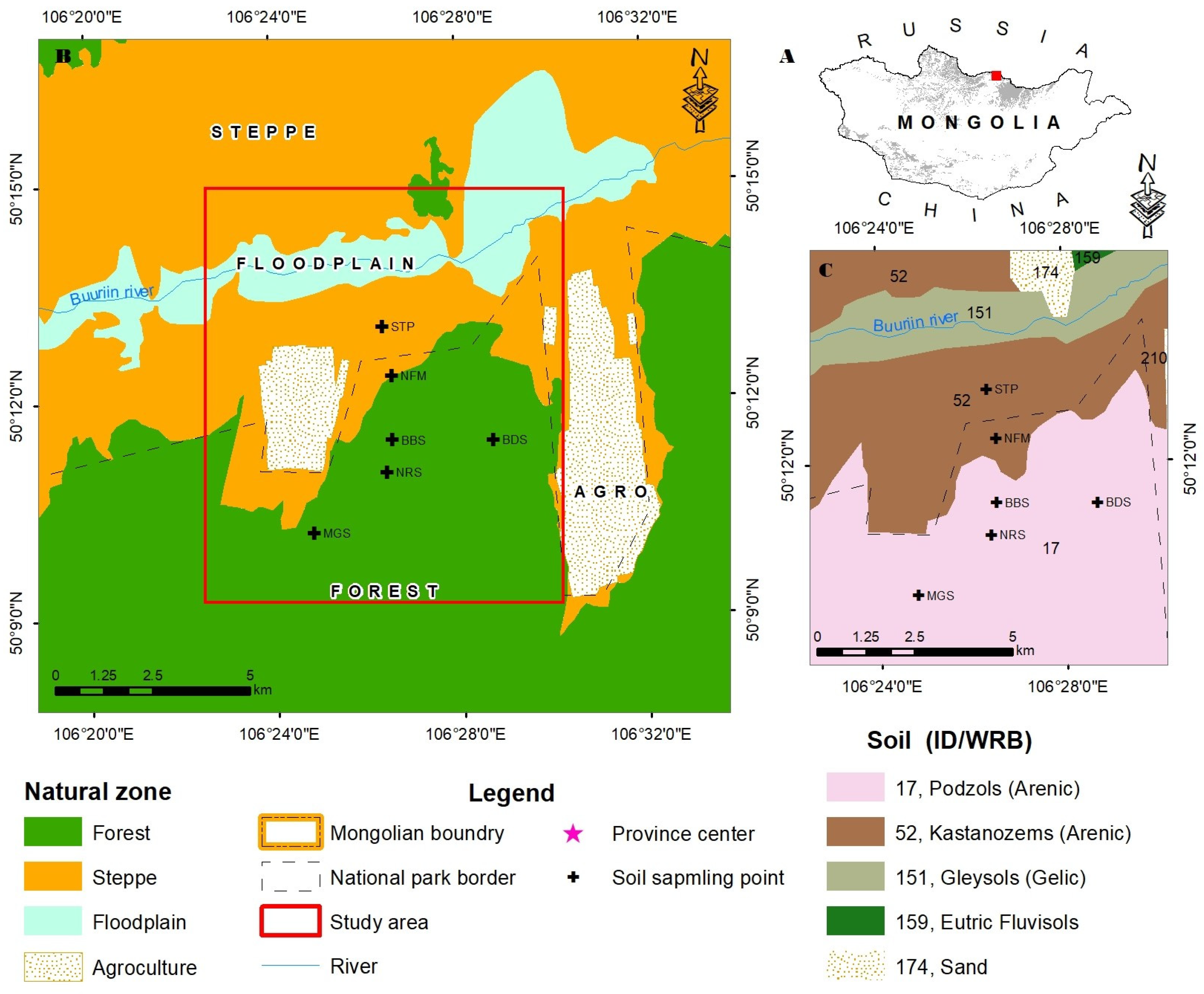
Figure 2.
Overview of the climatic conditions of the study area (meteorological station Sukhbaatar, 2003–2019); Climate diagram; illustrates the integrated representations of total precipitation and mean air temperature on a monthly basis.*Rome numbers described the month.
Figure 2.
Overview of the climatic conditions of the study area (meteorological station Sukhbaatar, 2003–2019); Climate diagram; illustrates the integrated representations of total precipitation and mean air temperature on a monthly basis.*Rome numbers described the month.
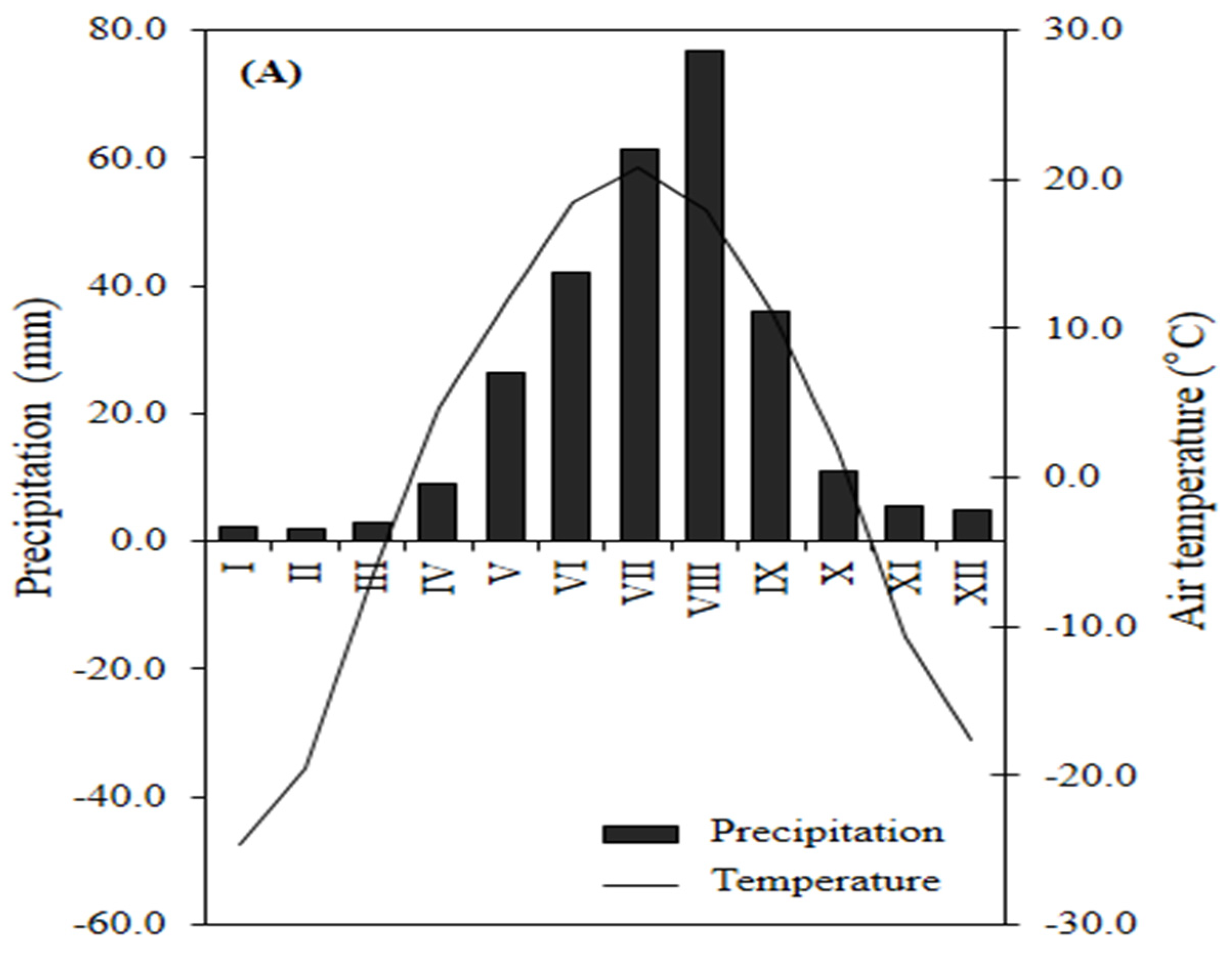
Figure 3.
The graphs demonstrate the relationship between species richness and plant coverage percentage across different plot types, suggesting an ecological study comparing different plots. Mean species richness, plant coverage and error bars indicate standard error of values in different plots. (a) Species richness (ranging from 0 to 40); (b) Plant coverage, % (0-80%).
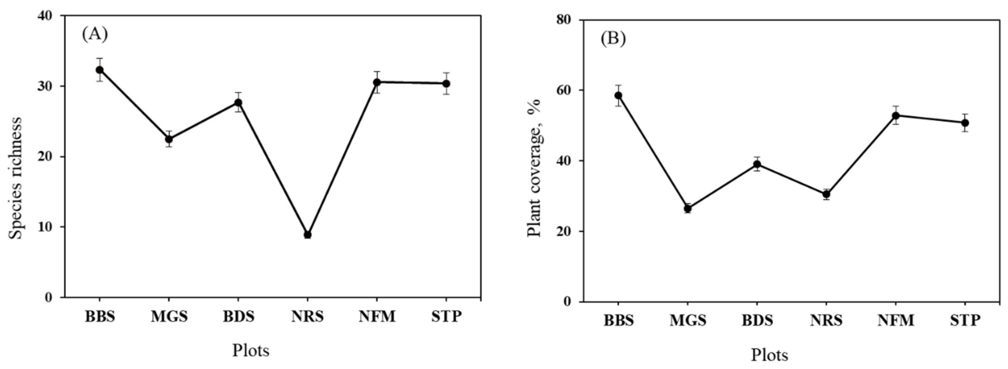
Figure 4.
The graphs show a consistent ratio between above- and below-ground biomass across plots and indicate variability or standard error for each plot. (a) Y-axis is an above-ground (g/m²), ranging from 0 to 140, (b) Y-axis: Below-ground biomass (g/m²), ranging from 0 to 4000 and X-axis: Different plot types: BBS, MGS, BDS, NRS, NFM, and STP.
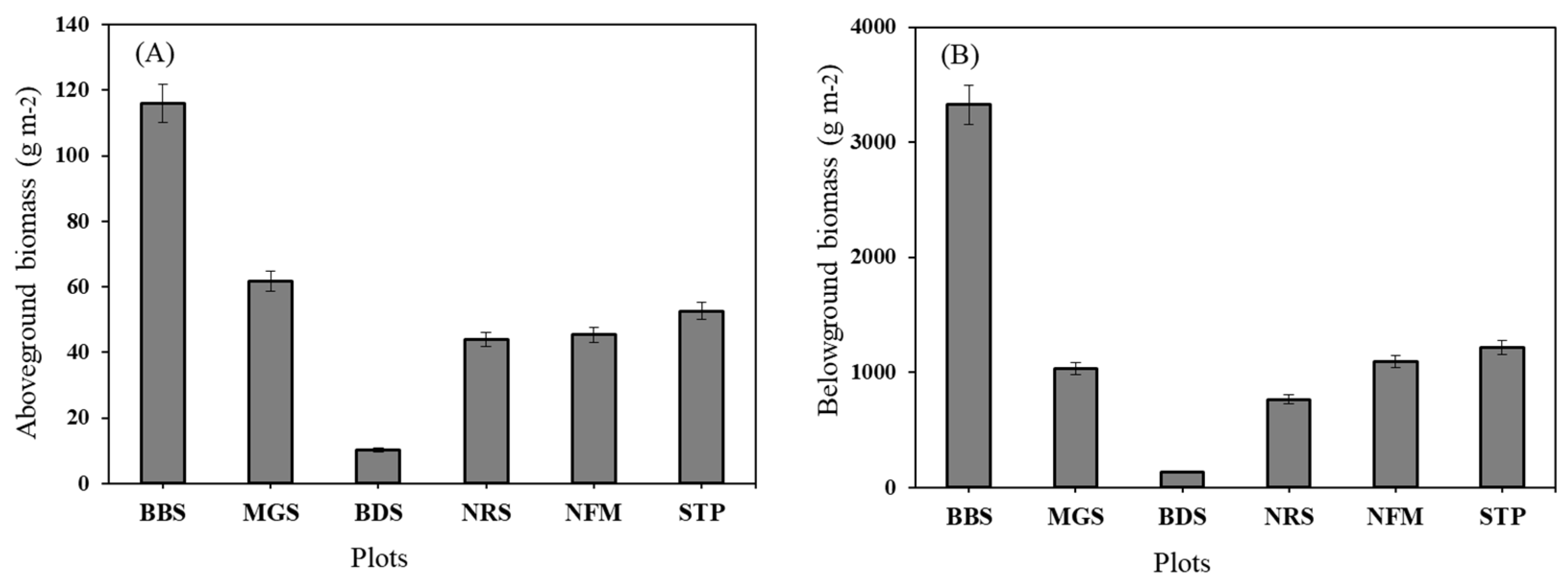
Figure 5.
(a) Component Analysis (PCA) biplot illustrates the correlations between variables and samples across two main components (Dim1 and Dim2), accounting for 33.2% and 18.2% of the variance, respectively. Arrows: Indicate variables (e.g., pH, Sand, Clay, Shannon's index, Evenness index, etc.). The orientation and magnitude of the arrows signify the influence of each variable on the principal components. Ellipses: Indicate clusters of samples (e.g., BBS, MGS, BDS, NRS, NFM, STP) according to their similarity. Principal component analysis and heatmap for vegetation and soil parameters under different plots (BBS, BDS, MGS, NFM, NRS, STP). (b) Heat-map of four vegetation parameters in six different plots. (c) Heat-map of twelve soil parameters in six different plots. This heatmap visualizes plant-related variables (species richness, vegetation cover, Shannon's index, and Evenness index) across different plots (BBS, MGS, BDS, NRS, color gradient: darker blue indicates higher values, while lighter blue indicates lower values.
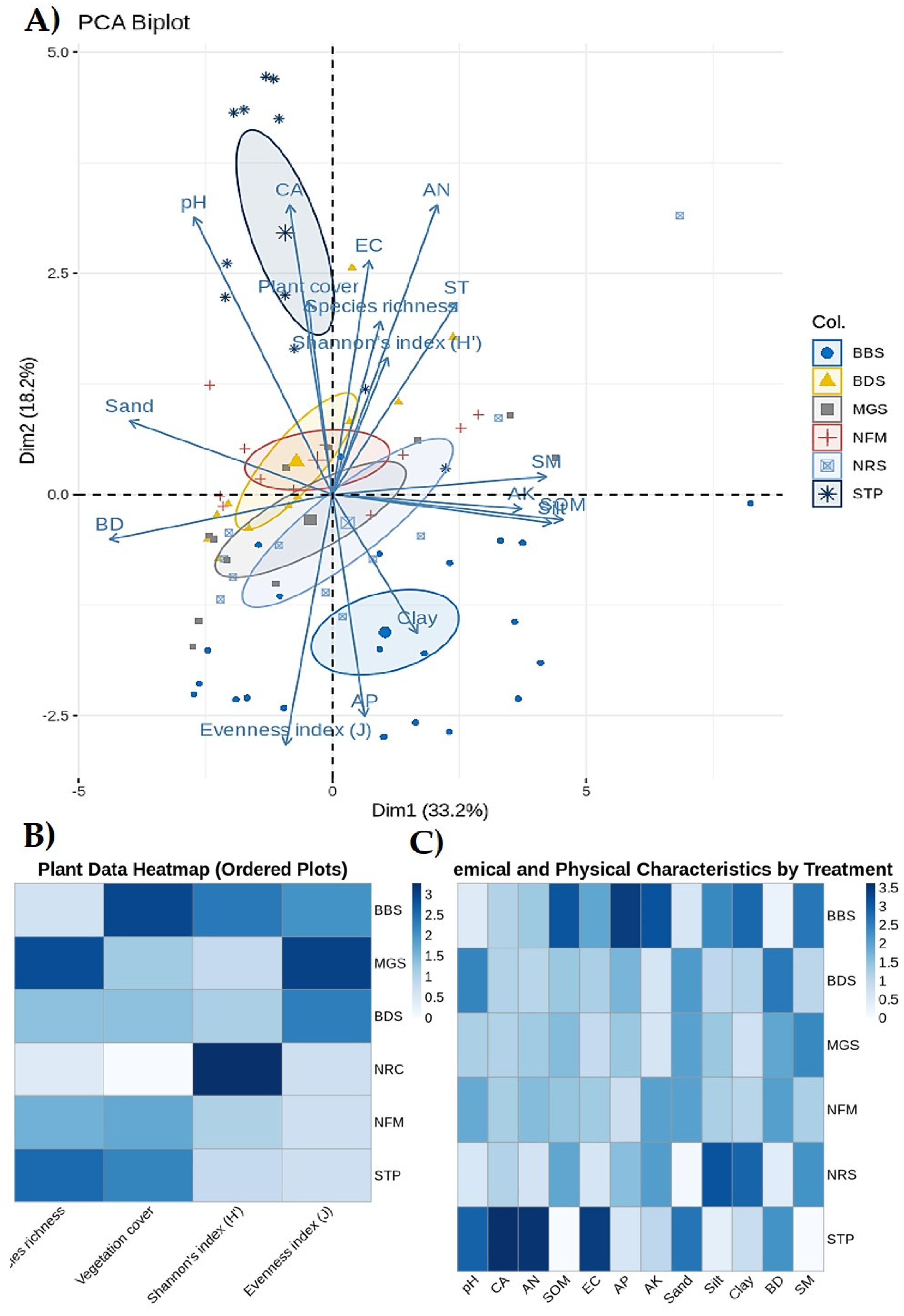
Figure 6.
Relationships between Shannon diversity index and soil properties across different plots. Shannon Index (H'): Ranges from 0.172 to 0.816; assesses species diversity by accounting for both richness and evenness. (a) Shannon vs pH: Ranges from 6.8 to 8.2; quantifies soil acidity and alkalinity. (b) Shannon versus SOM (%): Soil Organic Matter ranges from 15% to 35%, indicating organic content. (c) Shannon versus EC (dS/m): Electrical Conductivity ranges from 0.3 to 0.8 dS/m and quantifies soil salinity. *The blue shading denotes 95% confidence intervals, the trend lines illustrate linear regression fits, and the R² values reflect the proportion of variation explained.
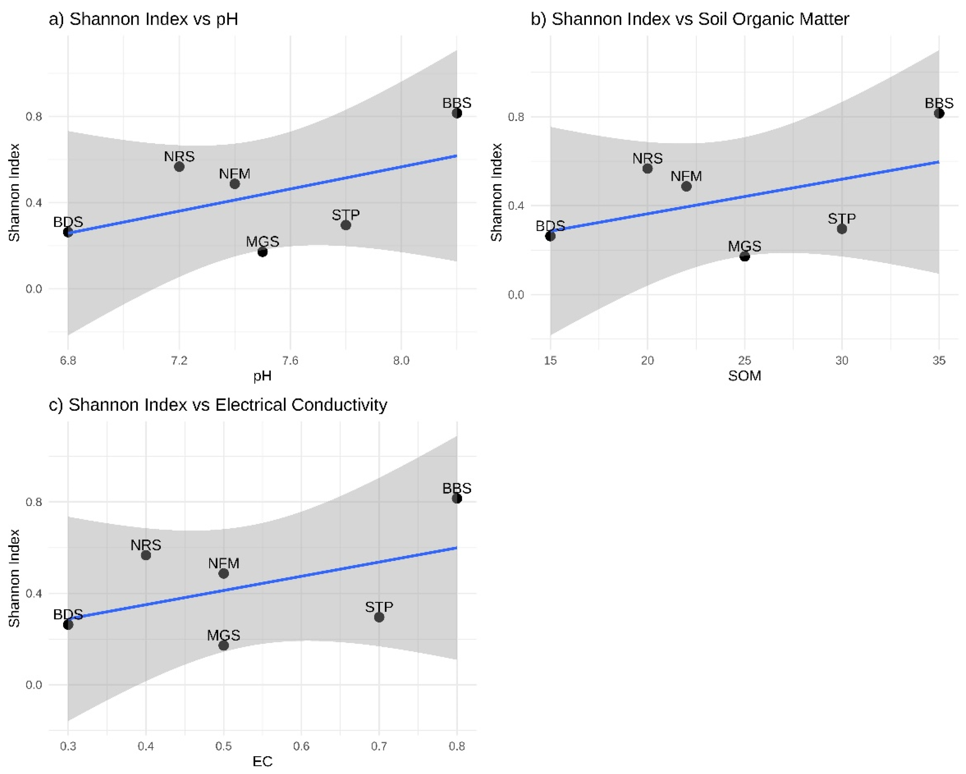

Table 1.
Geographical location of the sites.
| № | Plot ID | Plot definition | Coordinates | Altitude (m) | |
| 1 | BBS | 2003 plantation stand | N 50°11'26.7" | E 106°26'31.8" | 720 |
| 2 | MGS | 2004 plantation stand | N 50°10'10.6" | E 106°24'49.0" | 712 |
| 3 | BDS | 2005 plantation stand | N 50°11'25.4" | E 106°28'42.8" | 708 |
| 4 | NRS | Natural regeneration stand | N 50°10'59.9" | E 106°26'24.6" | 714 |
| 5 | NFM | Natural forest edge | N 50°14'7.45" | E 106°32'58.3" | 666 |
| 6 | STP | Steppe area | N 50°21'69.3" | E 106°43'92.9" | 624 |
Table 2.
Correlations between tree variables with species richness, plant coverage and above-below-ground biomass.
Table 2.
Correlations between tree variables with species richness, plant coverage and above-below-ground biomass.
| Variables | BBS | MGS | BDS | NRS | ||||||||||||
| SR | PC | AGB | BGB | SR | PC | AGB | BGB | SR | PC | AGB | BGB | SR | PC | AGB | BGB | |
| DBH | -0.14 | -0.11 | 0.5 | 0.5 | 0.21 | 0.21 | -0.5 | -0.51 | 0.16 | 0.16 | 0.48 | 0.59 | 0.38 | 0.31 | 0.03 | 0.26 |
| Height | -0.2 | -0.21 | 0.45 | 0.56 | 0.28 | 0.28 | -.619* | -0.59 | -0.1 | -0.1 | 0.04 | 0.21 | 0.3 | 0.43 | 0.16 | 0.39 |
| BA | -0.18 | -0.15 | 0.48 | 0.49 | 0.18 | 0.18 | -0.39 | -0.38 | 0.2 | 0.2 | 0.46 | 0.57 | 0.47 | 0.23 | -0.1 | 0.17 |
| Vol | -0.17 | -0.15 | 0.53 | 0.57 | 0.19 | 0.19 | -0.46 | -0.44 | 0.06 | 0.06 | 0.45 | 0.6 | 0.43 | 0.28 | -0.02 | 0.25 |
| CL | -0.2 | -0.15 | .627* | .653* | 0.4 | 0.4 | -0.57 | -0.56 | -0.33 | -0.34 | -0.02 | 0.14 | 0.29 | 0.42 | 0.16 | 0.41 |
| CD | 0.18 | 0.23 | -0.06 | -0.01 | 0.33 | 0.33 | -0.34 | -0.4 | 0.27 | 0.27 | 0.33 | 0.52 | 0.15 | 0.18 | 0.09 | 0.37 |
| CPA | 0.14 | 0.19 | -0.17 | -0.1 | -0.1 | -0.1 | -.637* | -.781** | 0.49 | 0.48 | 0.1 | 0.29 | 0.22 | 0.27 | 0.08 | 0.35 |
Note: *p < 0.05, **p < 0.01, vegetation variables: SR-species richness, PC-plant coverage, AGB-Above-ground biomass, BGB-below-ground biomass, tree variables: DBH – diameter at breast height, Height – tree height, BA – tree basal area, Vol – growing stock, CL – tree crown length, CD – tree crown diameter, CPA – crown projection area. Plots; BBS-2003 plantation stand, MGS-2004 plantation stand, BDS-2005 plantation stand, NRS- Natural regeneration stand.
Table 3.
Correlations between soil variables with species richness, plant coverage and above-below ground biomass of studied sample plots.
Table 3.
Correlations between soil variables with species richness, plant coverage and above-below ground biomass of studied sample plots.
| Variables | BBS | MGS | BDS | |||||||||
| SR | PC | AGB | BGB | SR | PC | AGB | BGB | SR | PC | AGB | BGB | |
| pH | 0.23 | 0.266 | -.645* | -.744** | -0.034 | -0.033 | -0.212 | -0.099 | -0.392 | -0.396 | -0.297 | -0.195 |
| SOC | -0.111 | -0.155 | 0.302 | 0.442 | -0.149 | -0.148 | 0.083 | 0.232 | -0.273 | -0.272 | 0.341 | 0.471 |
| BD | 0.23 | 0.266 | -.645* | -.744** | 0.096 | 0.095 | -0.078 | -0.23 | 0.34 | 0.333 | -0.382 | -0.45 |
| SM | -0.135 | -0.172 | -0.149 | -0.013 | -0.157 | -0.156 | 0.165 | 0.317 | -0.25 | -0.25 | 0.339 | 0.497 |
| Variables | NRS | NFM | STP | |||||||||
| SR | PC | AGB | BGB | SR | PC | AGB | BGB | SR | PC | AGB | BGB | |
| pH | -0.294 | -.616* | 0.122 | -0.094 | -0.425 | -0.252 | -0.126 | -0.238 | 0.162 | 0.268 | -0.227 | -0.371 |
| SOC | .657* | 0.447 | -0.222 | -0.082 | 0.517 | 0.235 | 0.241 | 0.376 | -0.095 | -0.217 | 0.315 | .439** |
| BD | -0.036 | -.749** | -0.529 | -.627* | -0.57 | -0.297 | -0.25 | -0.41 | -0.036 | 0.074 | -0.123 | -0.243 |
| SM | 0.35 | .683* | 0.184 | 0.309 | .609* | 0.328 | 0.27 | 0.396 | 0.205 | 0.085 | .411** | 0.468 |
Note: *p < 0.05, **p < 0.01, Vegetation variables: SR-species richness, PC-plant coverage, AGB-Above-ground biomass, BGB-below-ground biomass, soil variables: SOC – soil organic carbon, BD – soil bulk density, SM – soil moisture. Plots; BBS-2003 plantation stand, MGS-2004 plantation stand, BDS-2005 plantation stand, NRS- Natural regeneration stand, NFM-Natural forest edge, STP- Steppe area.
Table 4.
Quantitative analysis for IV of herbaceous vegetation in BBS, MGS and BDS plots.
| Plots | BBS | MGS | BDS | ||||||
| Species | RF, % | RC, % | IV, % | RF, % | RC, % | IV, % | RF, % | RC, % | IV, % |
| Achillea asiatica Serg. | 17 | 0.2 | 8.4 | 0 | 0 | 0 | 0 | 0 | 0 |
| Agrimonia pilosa Ledeb. | 17 | 2.1 | 9.4 | 0 | 0 | 0 | 0 | 0 | 0 |
| Artemisia commutata Bess. | 17 | 0.2 | 8.4 | 0 | 0 | 0 | 0 | 0 | 0 |
| Artemisia integrifolia L. | 17 | 1 | 8.9 | 0 | 0 | 0 | 0 | 0 | 0 |
| Cirsium esculentum (Siev.) C.A.Mey. | 0 | 0 | 0 | 0 | 0 | 0 | 4.8 | 2.4 | 3.6 |
| Cleistogenes squarrosa (Trinius) Keng. | 0 | 0 | 0 | 0 | 0 | 0 | 4.8 | 4.8 | 4.8 |
| Elymus sibiricus L. | 0 | 0 | 0 | 0 | 0 | 0 | 4.8 | 2.4 | 3.6 |
| Festuca valesiaca Gaud. | 17 | 2.1 | 9.4 | 0 | 0 | 0 | 0 | 0 | 0 |
| Galatella dahurica DC. | 17 | 1 | 8.9 | 0 | 0 | 0 | 0 | 0 | 0 |
| Heteropappus hispidus (Thunbg.) Less. | 17 | 1 | 8.9 | 0 | 0 | 0 | 4.8 | 2.4 | 3.6 |
| Iris tigrida Bunge ex Ledebour. | 0 | 0 | 0 | 0 | 0 | 0 | 4.8 | 2.4 | 3.6 |
| Leptopyrum fumarioides (L.) Reichb. | 0 | 0 | 0 | 0 | 0 | 0 | 4.8 | 1 | 2.9 |
| Linum sibiricum DC. | 17 | 2.1 | 9.4 | 0 | 0 | 0 | 0 | 0 | 0 |
| Papaver nudicaule Ldb. | 17 | 0.6 | 8.6 | 0 | 0 | 0 | 0 | 0 | 0 |
| Phlomis tuberosa L. | 0 | 0 | 0 | 7.1 | 2.7 | 4.9 | 4.8 | 2.4 | 3.6 |
| Potentilla acaulis L. | 0 | 0 | 0 | 0 | 0 | 0 | 4.8 | 2.4 | 3.6 |
| Sedum aizoon L. | 17 | 0.4 | 8.5 | 0 | 0 | 0 | 0 | 0 | 0 |
| Sibbaldia adpressa Bunge. | 0 | 0 | 0 | 7.1 | 5.4 | 6.3 | 0 | 0 | 0 |
| Trifolium lupinaster L. | 17 | 1 | 8.9 | 0 | 0 | 0 | 0 | 0 | 0 |
Note: *Vegetation variables: RF, %-relative frequency, RC, %-realtive coverage, IV, %-Importance Value. Plots: BBS-2003 plantation stand, MGS-2004 plantation stand, BDS-2005 plantation stand.
Table 5.
Quantitative analysis for IV of herbaceous vegetation in NRS, NFM and STP plots.
| Plots | NRS | NFM | STP | ||||||
| Species | RF, % | RC, % | IV, % | RF, % | RC, % | IV, % | RF, % | RC, % | IV, % |
| Allium bidentatum Fisch.ex.Prokh. | 0 | 0 | 0 | 10 | 6.3 | 8.2 | 0 | 0 | 0 |
| Allium linare L. | 0 | 0 | 0 | 0 | 0 | 0 | 13 | 2.6 | 7.5 |
| Caragana microphylla Lam. | 0 | 0 | 0 | 0 | 0 | 0 | 13 | 2.6 | 7.5 |
| Carum carvi L. | 0 | 0 | 0 | 10 | 1.6 | 5.8 | 0 | 0 | 0 |
| Cirsium esculentum (Siev.) C.A.Mey. | 0 | 0 | 0 | 0 | 0 | 0 | 13 | 1.3 | 6.9 |
| Cleistogenes squarrosa (Trinius) Keng. | 0 | 0 | 0 | 0 | 0 | 0 | 13 | 2.6 | 7.5 |
| Cymbaria dahurica L. | 0 | 0 | 0 | 0 | 0 | 0 | 13 | 1.8 | 7.2 |
| Elymus sibiricus L. | 10 | 8.9 | 9.4 | 0 | 0 | 0 | 0 | 0 | 0 |
| Festuca valesiaca Gaud. | 0 | 0 | 0 | 0 | 0 | 0 | 13 | 2.6 | 7.5 |
| Fragaria orientalis Losinsk. | 0 | 0 | 0 | 0 | 0 | 0 | 13 | 1.3 | 6.9 |
| Galatella dahurica DC. | 0 | 0 | 0 | 10 | 1.6 | 5.8 | 13 | 1.3 | 6.9 |
| Galium verum L. | 0 | 0 | 0 | 0 | 0 | 0 | 13 | 1.3 | 6.9 |
| Inula britannica L. | 0 | 0 | 0 | 0 | 0 | 0 | 13 | 0.3 | 6.4 |
| Leontopodium ochroleucum Beauverd. | 0 | 0 | 0 | 0 | 0 | 0 | 13 | 1.3 | 6.9 |
| Lespedeza davhurica (Laxm.) Schlinder. | 0 | 0 | 0 | 0 | 0 | 0 | 13 | 0.3 | 6.4 |
| Linum sibiricum DC. | 0 | 0 | 0 | 0 | 0 | 0 | 13 | 2.6 | 7.5 |
| Patrinia rupestris (Pall.) Dufr. | 0 | 0 | 0 | 0 | 0 | 0 | 13 | 5.1 | 8.8 |
| Phlomis tuberosa L. | 10 | 3.3 | 6.7 | 10 | 1.6 | 5.8 | 13 | 1.3 | 6.9 |
| Potentilla acaulis L. | 10 | 0 | 5 | 0 | 0 | 0 | 0 | 0 | 0 |
| Plantago major L. | 0 | 0 | 0 | 0 | 0 | 0 | 13 | 1.3 | 6.9 |
| Potentilla acaulis L. | 0 | 0 | 0 | 10 | 1.6 | 5.8 | 13 | 1.3 | 6.9 |
| Stellera chamaejasme (L.) Rydb. | 0 | 0 | 0 | 0 | 0 | 0 | 13 | 0.3 | 6.4 |
| Thalictrum petaloideum L. | 10 | 0.4 | 5.2 | 0 | 0 | 0 | 0 | 0 | 0 |
Note: *Vegetation variables: RF, %-relative frequency, RC, %-realtive coverage, IV, %-Importance Value. Plots: NRS- Natural regeneration stand, NFM-Natural forest edge, STP- Steppe area.
Table 6.
Species diversity indices of studied plots.
| Diversity indices | BBS | MGS | BDS | NRS | STP | NFM |
| Shannon index (H') | 0.8156a | 0.172c | 0.2632bc | 0.5671ab | 0.2959bc | 0.4871abc |
| Evenness index (J) | 0.1458cd | 0.4966b | 0.1720a | 0.1108cd | 0.2127c | 0.0869d |
| Simpson index (D) | 1.1638c | 0.5674ab | 0.7895a | 0.0855ab | 0.2988ab | 0.440bc |
*different letter indicate significant difference at 5%.
Table 7.
Similarity coefficients (%) of studied plots.
| Similarity coefficient, % | BBS, MGS, BDS, NRS | STP and NFM |
| Bray and Curtis (BC) | 0.30 | 0.28 |
| Sorensen (Ss) | 20.83 | 46.81 |
Table 8.
Soil properties comparison by depth (n=66).
| Variables | Unit | Soil depth (cm) | ANOVA statistic | |||
| 0-30 | 30-60 | 60-100 | MS | F value | ||
| pH | 6.70±0.09b | 7.01±0.07a | 7.01±0.06a | 0.85 | 34.8*** | |
| Carbonate (CaCO3) | % | 0.03±0.03c | 0.89±0.50a | 0.35±0.16b | 4.52 | 30.6*** |
| AN (N-NO-3) | mg kg-1 | 3.16±0.15a | 2.24±0.25b | 2.12±0.19b | 8.69 | 20.5*** |
| OC | g kg-1 | 10.1±1.00a | 3.7±0.39b | 1.4±0.09c | 54.37 | 60.6*** |
| SOCs | Mg ha-1 | 9.16±0.81a | 5.67±0.58b | 2.33±0.14c | 326.79 | 58.0*** |
| AP (P2O5) | mg kg-1 | 21.3±1.59b | 26.4±2.17a | 23.8±1.56ab | 16.02 | 4.0* |
| AK (K2O) | mg kg-1 | 114.6±9.79a | 79.4±2.76b | 74.8±2.39b | 1288.87 | 13.5*** |
| Sand (2-0.05 mm) | % | 72.9±1.41c | 77.9±1.19b | 86.6±0.44a | 1335.33 | 94.1*** |
| Silt (0.05-0.002 mm) | % | 15.1±1.16a | 9.0±0.7b | 3.8±0.24c | 883.58 | 72.5*** |
| Clay (<0.002 mm) | % | 12.0±0.59b | 13.0±0.57a | 9.5±0.37c | 81.83 | 30.0*** |
| BD | g cm-3 | 1.36±0.02c | 1.54±0.01b | 1.59±0.01a | 1.24 | 120.5*** |
| SM | % | 8.87±0.37a | 5.63±0.21b | 3.66±0.12c | 578.42 | 158.0*** |
| ST | 0C | 20.3±0.30a | 17.4±0.23b | 15.3±0.23c | 528.90 | 446.6*** |
Notes. Values are mean ± standard error, *p<0.05; **p<0.01; and ***p <0.001; Different letters within a row indicate significant differences (p<0.05) among the different treatments based on the one-way ANOVA result, followed by the Duncan’s multiple range test result. AN available nitrogen, AP available phosphorous, AK available potassium, OC organic carbon, SOCs- soil organic carbon stock, BD bulk density, SM soil moisture, ST soil temperature.
Table 9.
Soil properties of studied plots (n=48; depth=0-30 cm).
| Variables | Unit | BBS | NRS | STP | BDS | NFM | MGS | F value |
| pH | 6.10±0.11d | 6.51±0.07c | 7.00±0.47b | 7.39±0.03a | 6.77±0.13bc | 6.88±0.11bc | 13.14*** | |
| AN (N-NO-3) | mg kg-1 | 2.99±0.54ab | 4.07±0.62a | 2.88±0.58b | 3.17±0.58ab | 3.22±0.51ab | 3.56±0.81ab | 1.51ns |
| OC | g kg-1 | 26.7±12.89a | 14.6±7.52ab | 8.7±4.04b | 15.2±7.61ab | 15.8±3.53ab | 16.7±5.43ab | 1.8ns |
| SOCs | Mg ha-1 | 22.2±6.95a | 10.9±0.84bc | 8.1±1.51c | 14.5±3.02abc | 16.5±5.83ab | 15.3±4abc | 3.8* |
| AP (P2O5) | mg kg-1 | 26.4±9.32a | 17.3±4.42a | 20.1±7.37a | 23.9±5.99a | 14.7±5.34a | 21.2±8.69a | 1.1ns |
| AK (K2O) | mg kg-1 | 173.5±72.9a | 119.3±36.4ab | 108.5±35.5ab | 84.1±36.3b | 119.3±53.9ab | 94.9±27ab | 1.36ns |
| Sand (2-0.05mm) | % | 69.5±0.73b | 69.5±3.91b | 82.9±0.82a | 76.4±6.47ab | 75.9±6.93ab | 73.3±3.59b | 3.93* |
| Silt (0.05-0.002mm) | % | 19.8±1.94a | 17.9±7.54a | 8.4±1.59b | 11.6±4.89ab | 12.7±5.62ab | 15.3±3.71ab | 2.38ns |
| Clay (<0.002mm) | % | 10.8±1.32ab | 12.6±3.64a | 8.6±1.37b | 12±1.8ab | 11.4±1.74ab | 11.4±0.53ab | 1.48ns |
| BD | g cm-3 | 1.25±0.2a | 1.24±0.2a | 1.46±0.07a | 1.46±0.11a | 1.42±0.14a | 1.35±0.12a | 1.41ns |
| SM | % | 10.6±1.3a | 8.25±1.97ab | 5.15±2.23b | 7.97±2.72ab | 9.41±2.62ab | 12.06±4.33a | 2.35ns |
| ST | 0C | 18.65±1.62c | 17.74±0.74c | 24.68±2.56a | 21.22±0.85b | 21.53±1.27b | 18.09±0.94c | 9.96*** |
Notes. Values are mean ± standard deviation, *p<0.05; **p<0.01; and ***p <0.001; Different letters within a row indicate significant differences (p<0.05) among the different treatments based on the one-way ANOVA result, followed by the Duncan’s multiple range test result. AN available nitrogen, AP available phosphorous, AK available potassium, OC organic carbon, SOCs- soil organic carbon stock, BD bulk density, SM soil moisture, ST soil temperature.
Table 10.
Soil properties of studied plots (n=36; depth=30-60 cm).
| Variables | Unit | BBS | NRS | STP | BDS | NFM | MGS | F value |
| pH | 6.63±0.12e | 6.79±0.06d | 7.61±0.02a | 7.28±0.07b | 7.13±0.01c | 6.91±0.04d | 62.8*** | |
| AN (N-NO-3) | mg kg-1 | 2.64±0.7b | 1.58±0.18b | 4.29±1.44a | 1.73±0.38b | 2.03±0.18b | 1.81±0.18b | 4.45* |
| OC | g kg-1 | 9.97±1.48a | 6.38±1.46b | 2.19±0.45c | 5.93±1.64b | 6.02±2.16b | 5.14±0.75bc | 5.99** |
| SOCs | Mg ha-1 | 14.63±1.78a | 10.03±2.23b | 3.31±0.64c | 9.22±2.58b | 9.31±3.25b | 8.02±1.04b | 5.95** |
| AP (P2O5) | mg kg-1 | 39.19±1.74a | 31.81±3.62b | 14.03±3.87d | 24.07±2.07c | 17.66±1.2cd | 20.68±4.04cd | 19.9*** |
| AK (K2O) | mg kg-1 | 103.04±0a | 74.13±5.11b | 70.52±0b | 70.52±8.85b | 77.75±5.11b | 70.52±0b | 14.7*** |
| Sand (2-0.05mm) | % | 72.14±1.38c | 76.53±1.72c | 83.36±1.19a | 80.92±1.82ab | 79.46±3.01ab | 82.38±3.29a | 7.06** |
| Silt (0.05-0.002mm) | % | 12.69±1.38a | 9.56±0.66ab | 5.13±0.6c | 7.81±0.91bc | 8.93±2.45abc | 7.32±2.6bc | 4.71* |
| Clay (<0.002mm) | % | 15.17±0a | 13.91±1.23a | 11.52±0.6b | 11.27±0.91b | 11.61±0.7b | 10.3±0.69b | 11.2*** |
| BD | g cm-3 | 1.47±0.04b | 1.57±0.01a | 1.52±0.02ab | 1.55±0.02a | 1.55±0.02a | 1.57±0.03a | 4.56* |
| SM | % | 7.65±0.73a | 6.11±0.79b | 5.3±0.5b | 4.86±0.78bc | 4.44±0.83c | 3.96±0.38c | 7.5** |
| ST | 0C | 15.71±0.37b | 15.38±0.51b | 19.77±0.45a | 18.86±0.44a | 19.49±0.33a | 15.76±0.55b | 43.5*** |
Disclaimer/Publisher’s Note: The statements, opinions and data contained in all publications are solely those of the individual author(s) and contributor(s) and not of MDPI and/or the editor(s). MDPI and/or the editor(s) disclaim responsibility for any injury to people or property resulting from any ideas, methods, instructions or products referred to in the content. |
© 2025 by the authors. Licensee MDPI, Basel, Switzerland. This article is an open access article distributed under the terms and conditions of the Creative Commons Attribution (CC BY) license (http://creativecommons.org/licenses/by/4.0/).
Copyright: This open access article is published under a Creative Commons CC BY 4.0 license, which permit the free download, distribution, and reuse, provided that the author and preprint are cited in any reuse.


