
Submitted:
26 November 2025
Posted:
27 November 2025
You are already at the latest version
Abstract
Foundation models such as AlphaEarth introduce a new paradigm in remote sensing by providing semantically rich, pretrained embeddings that integrate multi-sensor, spatio-temporal, and contextual information. This study evaluates the performance of AlphaEarth embeddings for land-cover classification under both pixel-based and object-based paradigms within the Google Earth Engine (GEE) environment. Sentinel-2 imagery for 2024 was used to map a 1,930-hectare region in Pabbi Tehsil, Khyber Pakhtunkhwa, Pakistan, where rapid urbanization is reshaping traditional land use. Four experimental configurations—Pixel-Based Spectral Indices (PBSI), Pixel-Based AlphaEarth Embeddings (PBAE), Object-Based Spectral Indices (OBSI), and Object-Based AlphaEarth Embeddings (OBAE)—were implemented using a Random Forest classifier.The results show that AlphaEarth embeddings consistently outperformed spectral index–based models, improving overall accuracy by ≈ 5 percentage points and Kappa by ≈ 3. Object-based approaches enhanced spatial coherence and boundary delineation, particularly for built-up and road classes, while maintaining stable area statistics across pipelines. The findings demonstrate that pretrained embeddings can achieve deep-learning-level accuracy through lightweight, cloud-native workflows, offering an efficient pathway for land-cover mapping and urban-cadastral monitoring in data-scarce regions.
Keywords:
land-use/land-cover (LULC) classification
; alphaearth embeddings
; google earth engine
; pixel-based vs. object-based classification
; sentinel-2 imagery
; remote sensing in developing regions
Introduction:
Accurate and timely land-use and land-cover (LULC) information is fundamental for agricultural management, urban planning, environmental monitoring, and sustainable policymaking. LULC maps support decision-making in diverse domains including crop yield estimation, flood risk assessment, and monitoring of urban expansion [1]. They are also central to temporal change analysis, enabling long-term monitoring of deforestation, urban sprawl, and the dynamics of water bodies. In developing regions, LULC mapping plays a critical role in tracking the rapid conversion of agricultural land into urban settlements, thereby supporting policy interventions for food security and sustainable urban growth [2]. The increasing availability of free, high-resolution satellite imagery such as Sentinel-2 (10–20 m) [3], together with cloud-based geospatial platforms like Google Earth Engine (GEE) [4,5], has transformed LULC mapping by enabling reproducible, large-scale analyses without the burden of local data storage or preprocessing. Recent reviews highlight that foundation models are transforming remote sensing by enabling cross-sensor generalization and self-supervised feature learning [6,7]. As emphasized in Foundation Models for Earth Observation: Challenges and Perspectives (Nature Communications Earth & Environment, 2024), large-scale pretrained representations are becoming central to global mapping workflows. Despite these advances, most operational workflows still rely on traditional handcrafted indices for LULC mapping.
Traditional LULC classification approaches typically employ handcrafted indices such as NDVI and MNDWI [8,9], yet they suffer from mixed-pixel effects and frequently omit small or fragmented objects [10]. Techniques like Spectral Mixture Analysis (SMA) [11] and Multiple Endmember Spectral Mixture Analysis (MESMA) [12] can mitigate some of these issues but increase computational complexity and workflow difficulty. Water indices such as NDWI and MNDWI also perform inconsistently across varying backgrounds and are prone to confusion between shadows and bright objects, causing omission of small or fragmented water patches [13]. These challenges have accelerated the shift toward deep learning–based methods capable of learning abstract spatial and spectral features directly from data.
Recent advancements in deep learning (DL) particularly Convolutional Neural Networks (CNNs), Encoder–Decoder and Transformers, have driven remarkable progress in the semantic segmentation of remote sensing imagery, achieving state-of-the-art performance across scene classification, object detection, and change detection tasks [14]. For instance, transformer architectures trained on multi-temporal satellite data have demonstrated superior capabilities in modeling temporal dynamics of land-cover change [15]. Despite their success, deep learning architectures remain constrained by high computational demands, reliance on specialized hardware, and the need for large, annotated datasets, while their black-box nature limits interpretability and hinders policy-level adoption in operational land-cover mapping [16].
To further enhance classification consistency, embedding-based and semantic representation networks have recently been explored as alternatives to handcrafted indices [17]. The scalability of spectral indices is constrained by mixed-pixel effects and spectral confusion, while DL models remain hindered by computational demands, annotation requirements, and interpretability challenges. To bridge this gap, we evaluate the use of AlphaEarth embeddings [18], a globally available dataset of semantically rich, pre-computed feature vectors at 10 m resolution. These embeddings capture rich spatio-temporal and contextual information beyond the scope of handcrafted indices. This aligns with recent trends toward large-scale foundation models that integrate multimodal Earth observation data to produce transferable and semantically consistent features [19]. By coupling these embeddings with an efficient Random Forest (RF) classifier, we aim to combine the representational power of deep learning with the simplicity, scalability, and computational efficiency of traditional classifiers. Specifically, this study benchmarks AlphaEarth embeddings against the traditional spectral and object-based features (SNIC+GLCM) in a comprehensive framework, comparing both pixel-based and object-based classification paradigms within the Google Earth Engine (GEE) environment.
Study Area and Data:
Study Area :
The study area comprises a cluster of five revenue estates located in Pabbi Tehsil, District Nowshera, Khyber Pakhtunkhwa Province, Pakistan, covering a total area of approximately 1,930 hectares . The cluster lies adjacent to the Grand Trunk (GT) Road, which connects the provincial capital, Peshawar, with Islamabad. This region is agriculturally productive yet undergoing rapid urbanization, making it a suitable case study for evaluating land-cover classification methods. The dominant land uses include agricultural fields, residential built-up structures, and barren land. It is worth mentioning that the study area lacks any major water bodies—such as rivers, lakes, or ponds—and only contains narrow irrigation channels as shown in (Figure 1).
After applying cloud and data-quality masks to Sentinel-2 imagery, the effective mapped area used for classification was approximately 1,800 hectares, representing about 93 % of the total region of interest. This distinction is important because it clarifies that the unclassified portion corresponds to cloud-affected or low-quality pixels rather than omissions in model coverage.
According to official cadastral records from the 1928–29 land survey, the land was classified into six categories (Table 1), which have not been revised since. It is important to note that this historical dataset is presented solely for contextual understanding and was not used for classification validation. Ground-truth data for this study were instead generated through visual interpretation of high-resolution satellite imagery contemporaneous with the 2024 Sentinel-2 data.
At present, the on-ground situation has diverged significantly from the century-old cadastral record, posing challenges for effective urban planning, land taxation, and environmental management in the area.
Methodological Overview:
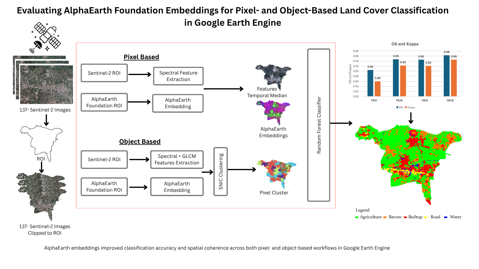
The workflow of this study comprised several key steps, including satellite image acquisition, preprocessing, temporal feature extraction, and validation of the Random Forest classification results using Overall Accuracy (OA), macro-averaged F1 score, and the Kappa coefficient (Figure 2). Four distinct classification pipelines were developed: (i) Pixel-Based Spectral Indices (PBSI), (ii) Pixel-Based AlphaEarth Embedding (PBAE), (iii) Object-Based Spectral Indices (OBSI), and (iv) Object-Based AlphaEarth Embedding (OBAE). These pipelines were designed to comprehensively assess the temporal, spectral, and embedding characteristics of the data for land cover classification.
Data Collection and Processing:
Sentinel-2 Level-2A imagery (13 spectral bands; 10–20 m spatial resolution) was accessed via the Google Earth Engine (GEE) platform for the period 1 January–31 December 2024. The collection COPERNICUS/S2_SR_HARMONIZED was filtered to the region of interest (ROI) and restricted to scenes with less than 10 % cloud cover. After applying these filters, a total of 137 cloud-free images were retained for further processing.
AlphaEarth Foundation Embeddings:
For the same period and ROI, AlphaEarth embeddings were accessed in GEE from the GOOGLE/SATELLITE_EMBEDDING/V1/ANNUAL dataset. Each 10 m pixel is represented by a 64-band feature vector (A00–A63) derived from the AlphaEarth Foundation model[18,20]. These embeddings integrate optical, radar, and temporal information to encode global land-surface dynamics in a compact feature space. Unlike traditional spectral inputs or vegetation indices, they capture multi-sensor and spatio-temporal relationships rather than isolated spectral responses. The embedding dataset was clipped to the 2024 calendar year and aligned spatially with the Sentinel-2 imagery to enable direct comparison of pixel- and object-based classification outputs.
Pixel-Based Feature Extractions:
For the pixel-based LULC workflow, several spectral indices were computed: Normalized Difference Vegetation Index (NDVI), Bare Soil Index (BSI), and Modified Normalized Difference Water Index (MNDWI). To enhance temporal stability, the mean and standard deviation of NDVI, as well as the mean of BSI and MNDWI, were calculated across the 2024 image collection. The final feature stack included [B2, B3, B4, B6, B8, NDVI_mean, NDVI_stdDev, BSI_mean, MNDWI_mean]. Bands B2, B3, B4, and B8 (10 m) were used for vegetation discrimination, while Band B6 (SWIR1, 20 m) was resampled to 10 m to support soil and built-up area separation. Pixel-based classification results are prone to the salt-and-pepper effect, which can be mitigated by object-based aggregation.
Object-Based Segmentation:
For the object-based analysis, Simple Non-Iterative Clustering (SNIC) segmentation was applied using B2, B3, B4, B8, and NDVI_mean as inputs. SNIC groups spectrally similar neighboring pixels into homogeneous clusters, generating a label image in which each pixel corresponds to a unique object. Texture information was derived from the Gray-Level Co-occurrence Matrix (GLCM) [21]. A grayscale composite was produced using luminance weights (0.299 × B8 + 0.587 × B4 + 0.114 × B3), and seven GLCM metrics were computed: Angular Second Moment, Contrast, Correlation, Entropy, Variance, Inverse Difference Moment, and Sum Average. These features describe local texture characteristics such as homogeneity, smoothness, and structural complexity. The final object-level feature set comprised [B2, B3, B4, B6, B8, NDVI_mean, NDVI_stdDev, BSI_mean, MNDWI_mean, gray_asm, gray_contrast, gray_corr, gray_ent, gray_var, gray_idm, gray_savg, cluster]. As an alternative, AlphaEarth embeddings provide a compact, information-rich representation for object-level classification.
Classification Framework
Training Data And Sampling:
Training data were prepared within the Google Earth Engine (GEE) environment through visual interpretation of high-resolution imagery available from the Google Satellite basemap, which primarily composites sub-meter to few-meter resolution data provided by Maxar and Airbus. Cadastral parcel boundaries were utilized as spatial references to guide sample delineation.
A total of 3,005 samples were collected across five land-use/land-cover (LULC) classes—Agriculture, Built-up, Barren, Road, and Water—representing the dominant land-cover types in the study area. Stratified random sampling was employed to ensure balanced class representation [22] with each class contributing approximately 600 samples. The dataset was divided into training (70 %; 2,135 samples) and validation (30 %; 870 samples) subsets, following common practice in remote sensing [23]. For pixel-based classification, training was conducted at the pixel level, while for object-based analysis, labels were assigned at the segment level to minimize within-object variability.
Classifier and Hyperparameters :
The Random Forest (RF) classifier was selected for its non-parametric nature, robustness to noisy predictors, and proven effectiveness in remote sensing applications [23,24]. Four experimental pipelines were evaluated: (i) pixel-based classification using spectral indices, (ii) pixel-based classification using AlphaEarth embeddings, (iii) object-based classification combining spectral indices with GLCM texture features, and (iv) object-based classification using AlphaEarth embeddings.
All experiments were implemented within the Google Earth Engine (GEE) environment. The RF classifier was configured with 500 decision trees to balance computational efficiency and predictive performance. For object-based analyses, GLCM texture features were derived using a 5 × 5 moving window. To identify optimal segmentation parameters, a parameter sweep was performed over SNIC seed and neighborhood size combinations. This sensitivity analysis quantified the effect of segmentation granularity on classification accuracy (OA) and agreement (Kappa).
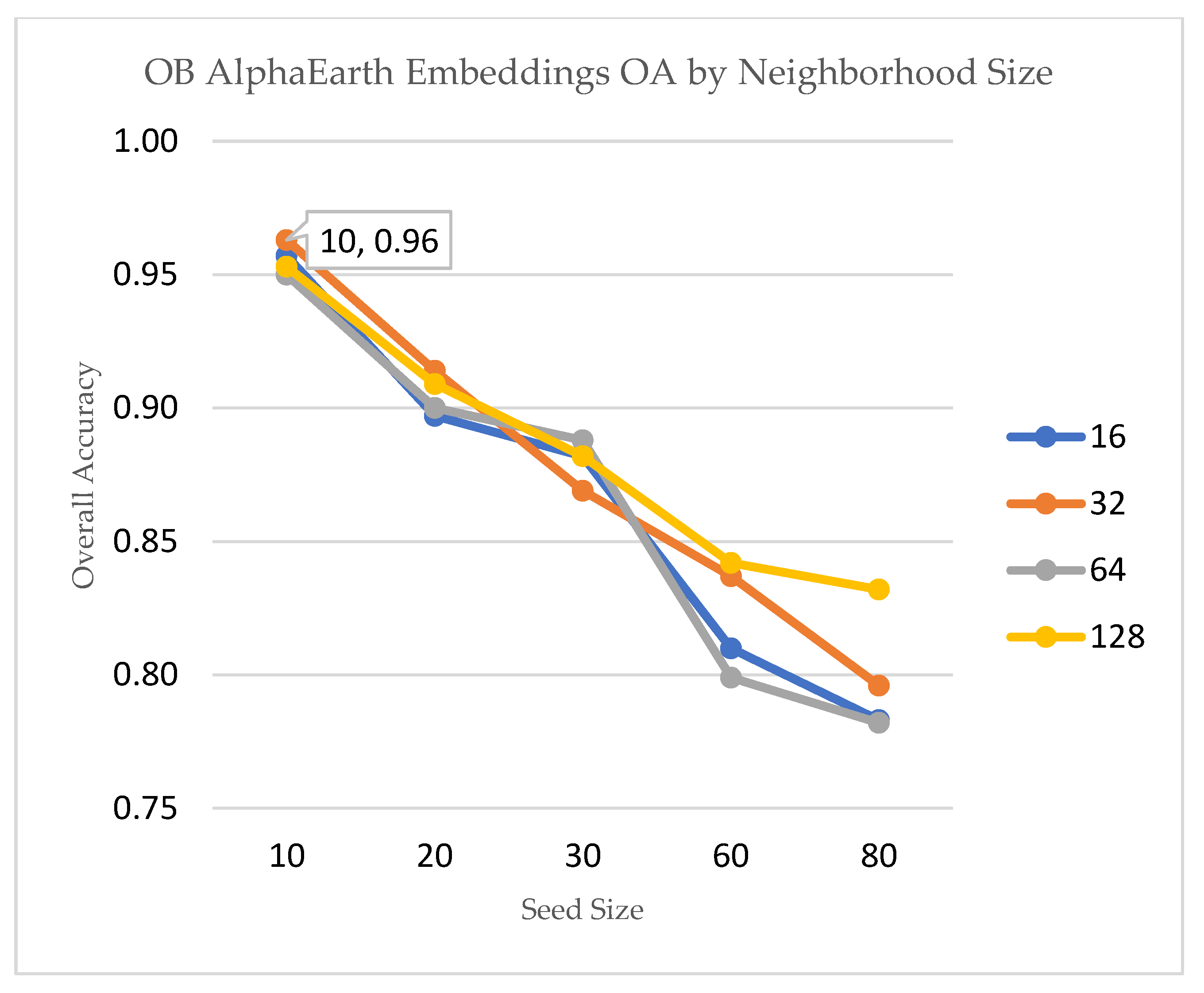
SNIC parameters were optimized separately for the spectral-index and embedding pipelines because the two input feature spaces have distinct spatial smoothness and intra-object homogeneity. We conducted a parameter sweep over seed spacing (10–80 m) and neighborhood size (16–128) and selected the settings that maximized validation OA under spatial cross-validation (seed=60, neighborhood=128 for spectral indices; seed=10, neighborhood=32 for embeddings). Table 2 summarizes the best performing parameter sets and Figure 3 provides the sensitivity plots for the two object-based pipelines.
Overall accuracy is plotted (see Figure 3a,b) against SNIC seed values, with neighborhood size represented by colored curves. The spectral-indices pipeline achieved the highest OA (0.95) at seed size 10 and neighborhood size 128, showing that finer segmentation improves boundary delineation but may introduce noise at higher seed values.
Figure 3.
(a): Sensitivity of object-based classification accuracy (OA) to SNIC parameters. Neighborhood size is plotted in 4 different colors.
Figure 3.
(a): Sensitivity of object-based classification accuracy (OA) to SNIC parameters. Neighborhood size is plotted in 4 different colors.
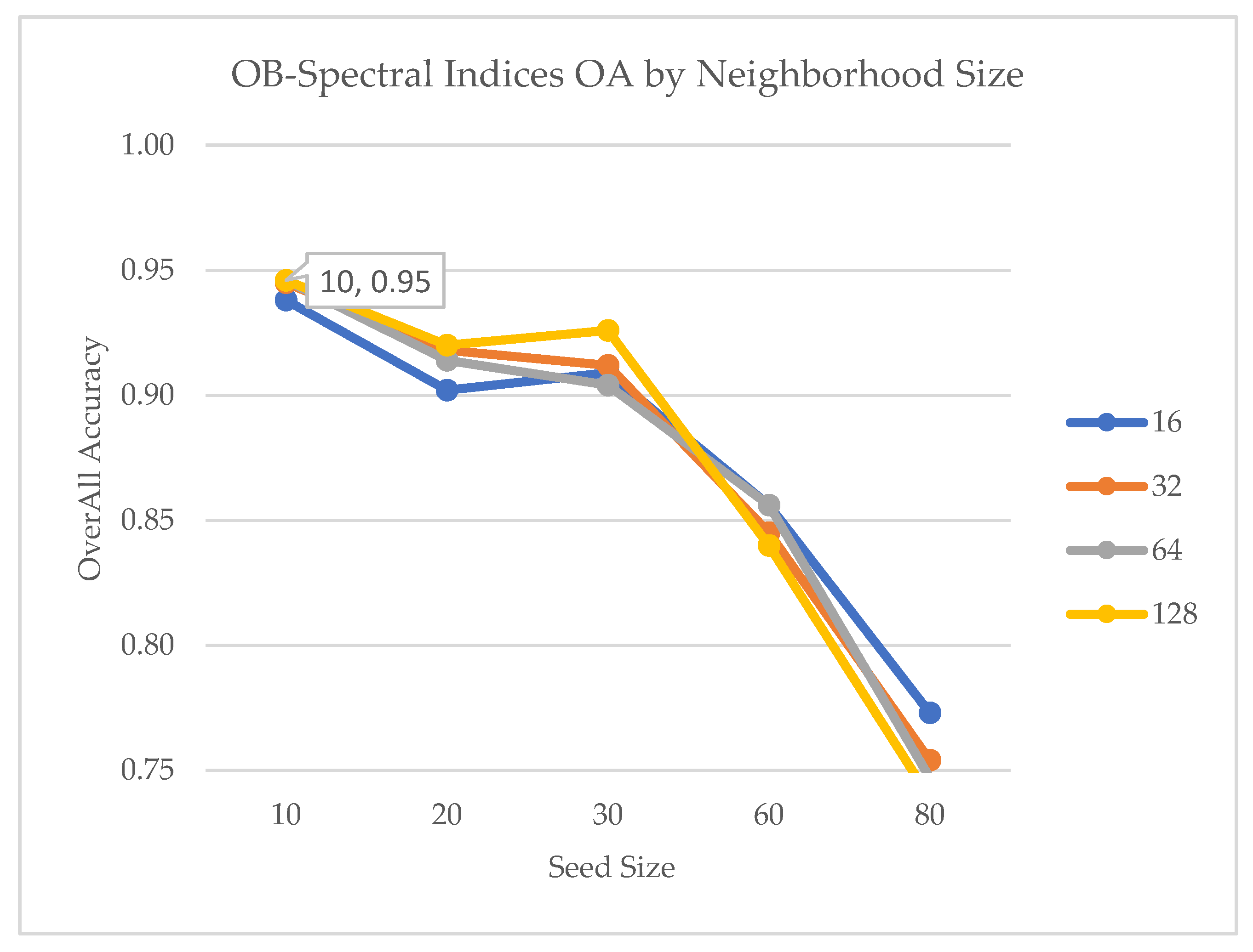
Figure 3.
(b): Sensitivity of object-based classification accuracy (OA) to SNIC parameters. Neighborhood size is plotted in 4 different colors.
Figure 3.
(b): Sensitivity of object-based classification accuracy (OA) to SNIC parameters. Neighborhood size is plotted in 4 different colors.
Results
The performance of each classification pipeline was evaluated using Overall Accuracy (OA), macro-averaged F1 score, and the Kappa coefficient. The F1 score represents the harmonic mean of User’s Accuracy (UA) and Producer’s Accuracy (PA)—equivalent to precision and recall in machine learning—and provides a balanced measure of per-class performance. The macro-average ensures equal weight for all land cover classes, minimizing bias caused by class imbalance.
The results demonstrate that the Object-Based AlphaEarth Embedding (OBAE) model achieved the highest performance, with 0.96 OA, 0.89 macro-F1, and 0.95 Kappa, outperforming all other pipelines (Figure 4 and Table 3).
The Pixel-Based Spectral Indices (PBSI) model yielded the lowest scores (0.90 OA, 0.79 macro-F1, 0.86 Kappa), while the AlphaEarth-based models (PBAE and OBAE) consistently outperformed the spectral index-based approaches in both pixel- and object-based frameworks (Table 3).
Class-Wise Performance:
At class level (Table 4), the PBAE pipeline improved classification consistency across all major land-cover types, particularly for built-up and road classes. Both pixel-based models showed reduced producer accuracy for water, likely due to limited training samples and confusion with shadowed or spectrally similar regions.
As shown in (Table 5), both object-based pipelines improved producer accuracies for vegetation and built-up classes. The AlphaEarth-based model provided better delineation of built-up and barren areas, while the spectral index-based model showed slightly higher precision for water and road features.
Across all configurations, object-based classification improved overall performance relative to pixel-based methods by reducing noise and enhancing class boundaries. The AlphaEarth embedding models (PBAE and OBAE) consistently achieved higher overall accuracy and F1 score than their spectral index counterparts. This indicates the potential of pretrained embedding features to generalize spatial patterns beyond the limitations of conventional spectral and index-based representations. Water remains the low performing class in both PBSI and OBSI because of the limited presence of water patches in the study area.
Visual Assessment:
The spatial patterns of the classified maps are shown in (Figure 5 and Figure 6). Embedding-based outputs(Figure 5g) produced smoother land-cover maps with reduced salt-and-pepper noise compared to spectral index pipelines (Figure 5c). This was particularly evident in heterogeneous areas, where object-based embedding classification(Figure 6d) further enhanced boundary delineation and improved representation of linear features such as roads.
Area Statistics:
The class-wise area estimates derived from the four pipelines show consistent totals of approximately 1800 hectare across all configurations, corresponding to ≈ 93 % of the 1930-hectare ROI after cloud masking. Minor discrepancies (< 1 %) between spectral- and embedding-based totals arise from differences in data completeness and segmentation boundary effects. Table 7a summarizes the class-wise area estimates obtained from the pixel-based (PBSI) and object-based (OBSI) pipelines using spectral indices.

Table 6.
a). Class-wise area (ha) derived from spectral index-based pipelines (PBSI, OBSI).
| Class | PBSI Area (ha) | OBSI Area (ha) |
| Agriculture | 1032.51 | 1152.26 |
| Barren | 344.7 | 210.56 |
| Built-up | 368.39 | 363.78 |
| Road | 32.83 | 39.76 |
| Water | 17.58 | 32.46 |
| Total | 1796.01 | 1798.82 |
Similarly, Table 6b reports the corresponding results for the embedding-based approaches (PBAE, OBAE).
Table 6.
b. Class-wise area (ha) derived from embedding-based pipelines (PBAE, OBAE).
| Class | PBAE Area (ha) | OBAE Area (ha) |
| Agriculture | 1160.09 | 1224.6 |
| Barren | 215.98 | 166.85 |
| Built-up | 407.81 | 328.69 |
| Road | 23.4 | 71.37 |
| Water | 2.24 | 18.02 |
| Total | 1809.53 | 1809.53 |
The AlphaEarth embedding datasets are pre-harmonized and gap-filled, resulting in a slightly larger valid-pixel coverage than Sentinel-2 spectral indices, which exclude cloudy or low-quality observations. Consequently, the embedding-based pipelines (PBAE, OBAE) report marginally higher total mapped area than the spectral-index pipelines (PBSI, OBSI), while maintaining nearly identical proportional class distributions.
Discussion:
This study evaluated conventional spectral index–based and AlphaEarth embedding–based Random Forest pipelines under both pixel- and object-based paradigms, highlighting how foundation embeddings reshape land-cover mapping. The results confirm that pretrained multi-sensor embeddings deliver consistent performance gains, especially in heterogeneous urban environments where spectral indices often suffer from confusion between built-up, road, and barren classes.
The area statistics (tables 6a–6b) indicate that both spectral and embedding-based pipelines produced comparable total mapped areas (~1,800 ha, ≈93 % of the 1,930 ha ROI), suggesting minimal geometric distortion across classification paradigms. Slightly higher coverage from embedding-based models reflects their gap-filled and harmonized nature, confirming their utility for operational mapping under cloud-affected conditions.
Technically, AlphaEarth embeddings derive their advantage from a cross-sensor, spatio-temporal learning framework that integrates optical, radar, and topographic information. Unlike handcrafted spectral indices that rely on fixed reflectance ratios, embeddings encode richer spectral–spatial representations, capturing fine-grained textures, edge continuity, and contextual relationships between neighboring land-cover types. This representation richness allows the classifier to distinguish spectrally similar but semantically distinct surfaces, such as barren fields and built-up structures, with greater reliability. Furthermore, embeddings generalize spatial patterns learned from global-scale training data, providing robustness to illumination changes, seasonal variation, and local noise—factors that often degrade traditional index-based models. These properties explain the smoother, more coherent land-cover maps and improved delineation of built-up and road features.
Consistent improvements in overall accuracy, F1, and Kappa demonstrate that pretrained embeddings generalize effectively even with limited training samples. From an application standpoint, the gains in urban and road delineation are particularly relevant for cadastral updating and land administration in semi-arid regions such as Pabbi, where built surfaces, bare soil, and seasonal vegetation frequently overlap within small parcels. Embedding-based pipelines improved boundary precision and reduced intra-class variability, yielding cartographically stable outputs suitable for urban growth monitoring and land-use planning. Conversely, both pipelines exhibited lower accuracy for water classes due to the scarcity and narrow geometry of irrigation channels in the study area. This limitation reflects the actual land-cover composition rather than a systematic model weakness.
Parameter sensitivity experiments also revealed that SNIC segmentation is scale dependent. Optimal configurations differed between the two feature domains, reflecting their inherent spatial variance. The finer segmentation (seed = 10, neighborhood = 32) observed for embeddings corresponds to their higher spatial information density, whereas spectral indices required coarser aggregation (seed = 10, neighborhood = 128) to suppress intra-class noise. These findings underscore the importance of scale-aware tuning when applying object-based methods across heterogeneous feature spaces.
Conclusion:
AlphaEarth embeddings consistently outperformed traditional spectral indices across both pixel- and object-based Random Forest pipelines, improving overall accuracy by up to 5 % and Kappa by 3 %. Their pretrained, multi-sensor representation enhanced delineation of built-up and road classes and maintained stable class-wise area estimates within ±1 % of the total mapped region. Object-based segmentation further improved spatial coherence and reduced noise, demonstrating that embedding-based approaches are operationally robust for cadastral updating and urban land monitoring.
These results underscore the potential of foundation embeddings to provide accuracy comparable to deep-learning approaches through scalable, cloud-native workflows such as Google Earth Engine, without the computational overhead of end-to-end neural training. The approach offers a practical pathway for national mapping agencies and land administration authorities to modernize land information systems using open-access data and reproducible AI pipelines.
Future work will integrate AlphaEarth embeddings with U-Net and SAM architectures for parcel-level change detection.
Limitations and Future Work:
Although AlphaEarth embeddings significantly improved classification accuracy, some limitations remain. The 10 m Sentinel-2 resolution constrains the detection of narrow features such as irrigation channels and smallholder field boundaries. Moreover, the pretrained embedding model was developed for general-purpose Earth observation and not specifically optimized for agricultural or cadastral contexts, which may limit sensitivity to subtle land-cover transitions. Future work should explore fine-tuning or domain adaptation using regional training data to enhance class separability and local relevance.
The rich spatial–contextual representations of AlphaEarth embeddings also offer potential for agricultural field boundary extraction. Combining them with higher-resolution imagery or multi-temporal features could enable more precise parcel delineation and support scalable land-use monitoring and cadastral updating in diverse agro-ecological regions.
Supplementary Materials
Acknowledgments
We want to extend our sincere thanks to Google for freely providing Sentinel-2, and AlphaEarth Embedding datasets integrated in Google Earth Engine. This research has received no funding.
Conflicts of Interest
The authors declare no conflict of interest.
References
- Talukdar, S.; Singha, P.; Mahato, S.; Shahfahad; Pal, S. ; Liou, Y.A.; Rahman, A. Land-Use Land-Cover Classification by Machine Learning Classifiers for Satellite Observations-A Review. Remote Sens. 2020, 12. [Google Scholar]
- Basheer, S.; Wang, X.; Farooque, A.A.; Nawaz, R.A.; Liu, K.; Adekanmbi, T.; Liu, S. Comparison of Land Use Land Cover Classifiers Using Different Satellite Imagery and Machine Learning Techniques. Remote Sens. 2022, 14. [Google Scholar] [CrossRef]
- Drusch, M.; Del Bello, U.; Carlier, S.; Colin, O.; Fernandez, V.; Gascon, F.; Hoersch, B.; Isola, C.; Laberinti, P.; Martimort, P.; et al. Sentinel-2: ESA’s Optical High-Resolution Mission for GMES Operational Services. Remote Sens. Environ. 2012, 120, 25–36. [Google Scholar] [CrossRef]
- Gorelick, N.; Hancher, M.; Dixon, M.; Ilyushchenko, S.; Thau, D.; Moore, R. Google Earth Engine: Planetary-Scale Geospatial Analysis for Everyone. Remote Sens. Environ. 2017, 202, 18–27. [Google Scholar] [CrossRef]
- Amani, M.; Ghorbanian, A.; Ahmadi, S.A.; Kakooei, M.; Moghimi, A.; Mirmazloumi, S.M.; Moghaddam, S.H.A.; Mahdavi, S.; Ghahremanloo, M.; Parsian, S.; et al. Google Earth Engine Cloud Computing Platform for Remote Sensing Big Data Applications: A Comprehensive Review. IEEE J. Sel. Top. Appl. Earth Obs. Remote Sens. 2020, 13, 5326–5350. [Google Scholar] [CrossRef]
- Huo, C.; Chen, K.; Zhang, S.; Wang, Z.; Yan, H.; Shen, J.; Hong, Y.; Qi, G.; Fang, H.; Wang, Z. When Remote Sensing Meets Foundation Model: A Survey and Beyond. Remote Sens. 2025, 17, 179. [Google Scholar] [CrossRef]
- Xiao, A.; Xuan, W.; Wang, J.; Huang, J.; Tao, D.; Lu, S.; Yokoya, N. Foundation Models for Remote Sensing and Earth Observation: A Survey. IEEE Geosci. Remote Sens. Mag. 2024. [Google Scholar] [CrossRef]
- Lu, D.; Weng, Q. A Survey of Image Classification Methods and Techniques for Improving Classification Performance. Int. J. Remote Sens. 2007, 28, 823–870. [Google Scholar] [CrossRef]
- Tassi, A.; Vizzari, M. Object-Oriented Lulc Classification in Google Earth Engine Combining Snic, Glcm, and Machine Learning Algorithms. Remote Sens. 2020, 12, 1–17. [Google Scholar] [CrossRef]
- Phiri, D.; Simwanda, M.; Salekin, S.; Nyirenda, V.R.; Murayama, Y.; Ranagalage, M. Sentinel-2 Data for Land Cover/Use Mapping: A Review. Remote Sens. 2020, 12. [Google Scholar] [CrossRef]
- Clark, M.L. Comparison of Simulated Hyperspectral HyspIRI and Multispectral Landsat 8 and Sentinel-2 Imagery for Multi-Seasonal, Regional Land-Cover Mapping. Remote Sens. Environ. 2017, 200, 311–325. [Google Scholar] [CrossRef]
- Degerickx, J.; Roberts, D.A.; Somers, B. Enhancing the Performance of Multiple Endmember Spectral Mixture Analysis (MESMA) for Urban Land Cover Mapping Using Airborne Lidar Data and Band Selection. Remote Sens. Environ. 2019, 221, 260–273. [Google Scholar] [CrossRef]
- Acharya, T.D.; Subedi, A.; Lee, D.H. Evaluation of Water Indices for Surface Water Extraction in a Landsat 8 Scene of Nepal. Sensors (Basel) 2018, 18, 2580. [Google Scholar] [CrossRef] [PubMed]
- Huang, L.; Jiang, B.; Lv, S.; Liu, Y.; Fu, Y. Deep-Learning-Based Semantic Segmentation of Remote Sensing Images: A Survey. IEEE J. Sel. Top. Appl. Earth Obs. Remote Sens. 2024, 17, 8370–8396. [Google Scholar] [CrossRef]
- Voelsen, M.; Rottensteiner, F.; Heipke, C. Transformer Models for Land Cover Classification with Satellite Image Time Series. PFG – J. Photogramm. Remote Sens. Geoinf. Sci. 2024, 92, 547–568. [Google Scholar] [CrossRef]
- Dimitrovski, I.; Kitanovski, I.; Simidjievski, N.; Kocev, D. In-Domain Self-Supervised Learning Improves Remote Sensing Image Scene Classification. IEEE Geosci. Remote Sens. Lett. 2024, 21. [Google Scholar] [CrossRef]
- Chen, J.; Du, X.; Zhang, J.; Wan, Y.; Zhao, W. SEMANTIC KNOWLEDGE EMBEDDING DEEP LEARNING NETWORK FOR LAND COVER CLASSIFICATION. Int. Arch. Photogramm. Remote Sens. Spatial Inf. Sci. 2023, XLVIII-1-W2-2023, 85–90. [Google Scholar] [CrossRef]
- Brown, C.F.; Kazmierski, M.R.; Pasquarella, V.J.; Rucklidge, W.J.; Samsikova, M.; Zhang, C.; Shelhamer, E.; Lahera, E.; Wiles, O.; Ilyushchenko, S.; et al. AlphaEarth Foundations: An Embedding Field Model for Accurate and Efficient Global Mapping from Sparse Label Data. 2025.
- Lu, S.; Guo, J.; Zimmer-Dauphinee, J.R.; Nieusma, J.M.; Wang, X.; VanValkenburgh, P.; Wernke, S.A.; Huo, Y. Vision Foundation Models in Remote Sensing: A Survey. OpenReview 2024. [Google Scholar] [CrossRef]
- Satellite Embedding V1 | Earth Engine Data Catalog | Google for Developers. Available online: https://developers.google.com/earth-engine/datasets/catalog/GOOGLE_SATELLITE_EMBEDDING_V1_ANNUAL#citations (accessed on 20 September 2025).
- Haralick, R.M.; Dinstein, I.; Shanmugam, K. Textural Features for Image Classification. IEEE Trans. Syst. Man Cybern. 1973, SMC-3, 610–621. [Google Scholar] [CrossRef]
- Foody, G.M. Status of Land Cover Classification Accuracy Assessment. Remote Sens. Environ. 2002, 80, 185–201. [Google Scholar] [CrossRef]
- Belgiu, M.; Drăgu, L. Random Forest in Remote Sensing: A Review of Applications and Future Directions. ISPRS J. Photogramm. Remote Sens. 2016, 114, 24–31. [Google Scholar] [CrossRef]
- Rodriguez-Galiano, V.F.; Ghimire, B.; Rogan, J.; Chica-Olmo, M.; Rigol-Sanchez, J.P. An Assessment of the Effectiveness of a Random Forest Classifier for Land-Cover Classification. ISPRS J. Photogramm. Remote Sens. 2012, 67, 93–104. [Google Scholar] [CrossRef]
Figure 1.
OpenStreetMap view of the Study Area.
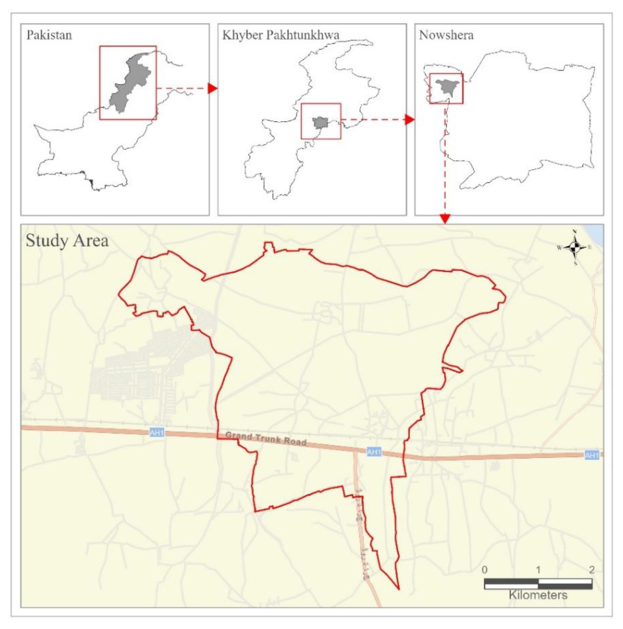
Figure 2.
Methodological workflow
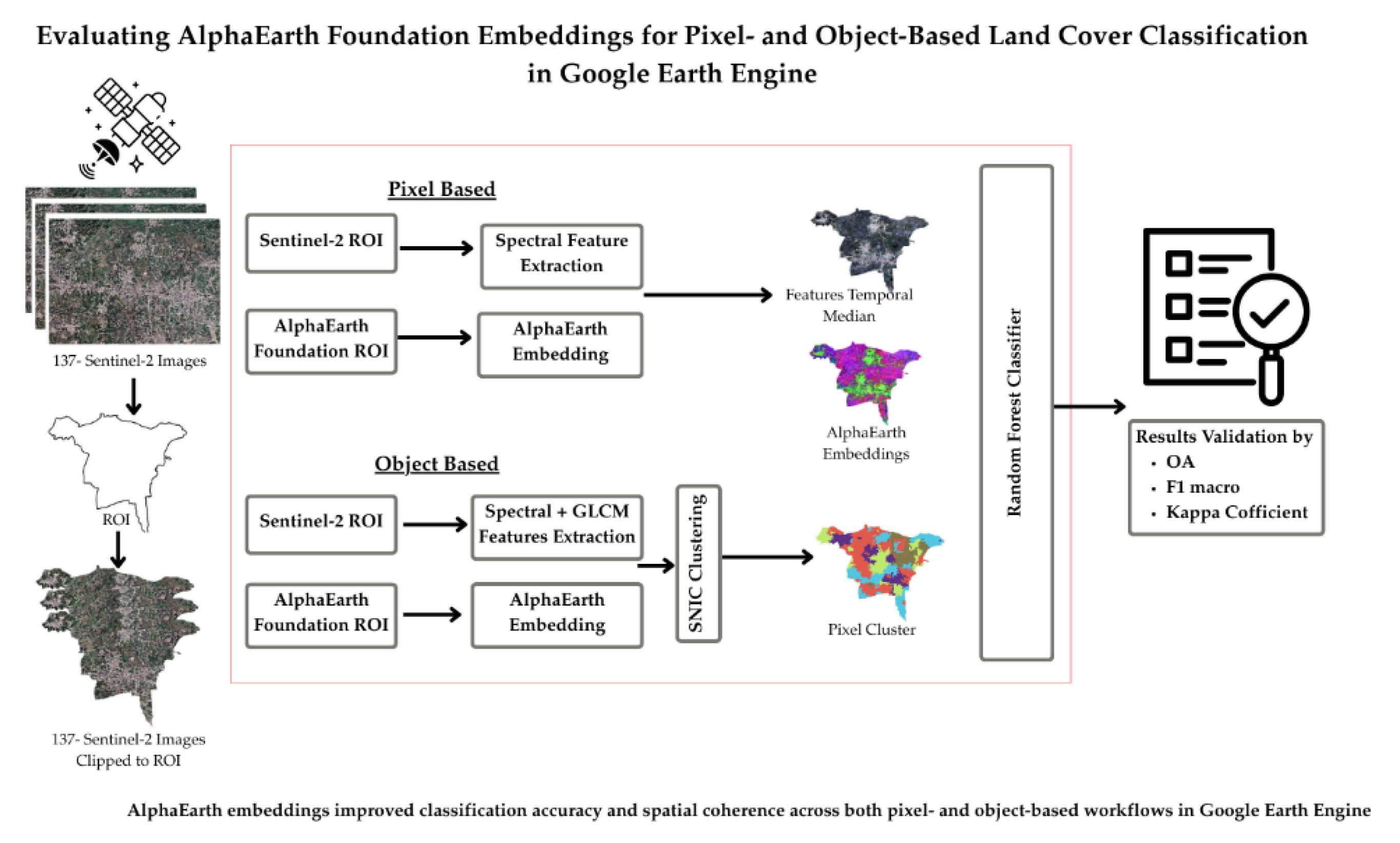
Figure 4.
Comparison of Overall Accuracy (OA), macro-averaged F1 score, and Kappa coefficient across pixel-based and object-based classification pipelines.
Figure 4.
Comparison of Overall Accuracy (OA), macro-averaged F1 score, and Kappa coefficient across pixel-based and object-based classification pipelines.
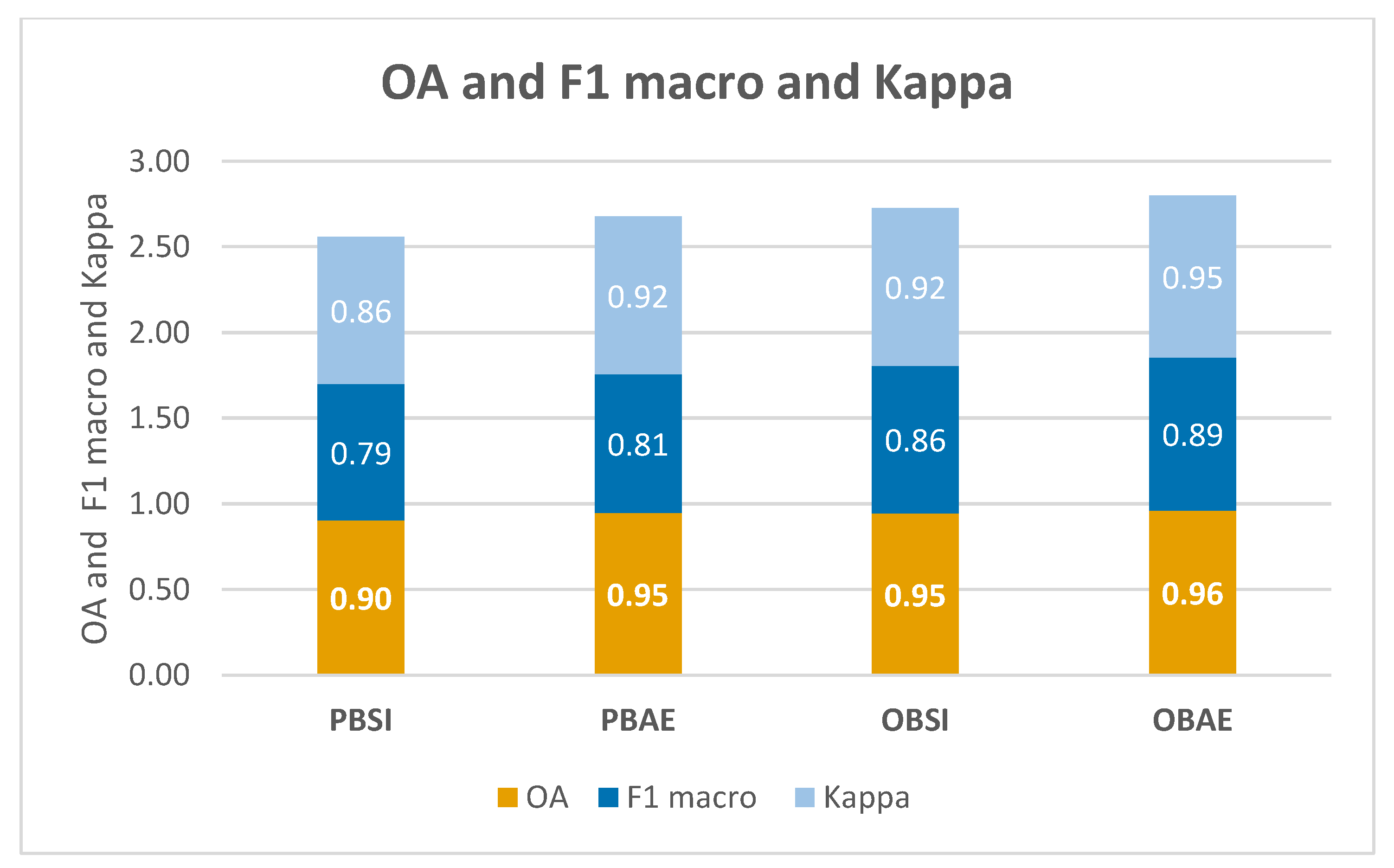
Figure 5.
(a) RGB, (b)Spectral Indices(SI) median, (c) PBSI Classified (d) RGB (e) AlphaEarth Embedding (AE) (g) PBAE Classified Image.
Figure 5.
(a) RGB, (b)Spectral Indices(SI) median, (c) PBSI Classified (d) RGB (e) AlphaEarth Embedding (AE) (g) PBAE Classified Image.
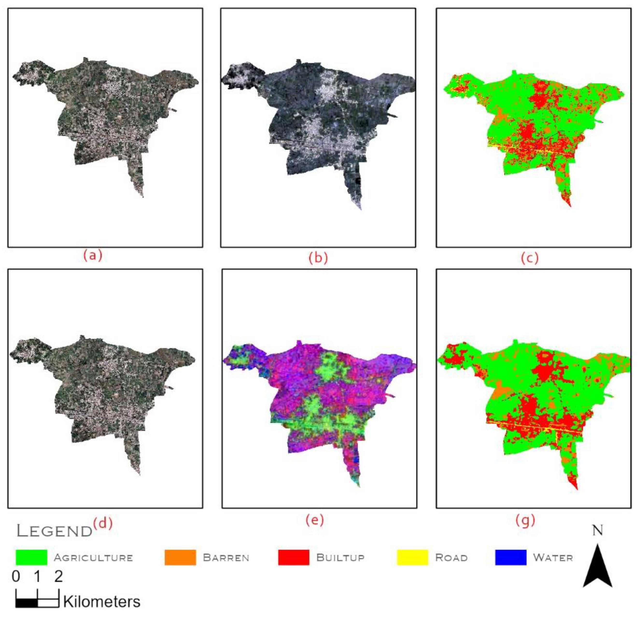
Figure 6.
(a) SNIC segmentation (b) OBSI classified Image (c) AE Embedding (d) OBAE classified Image.
Figure 6.
(a) SNIC segmentation (b) OBSI classified Image (c) AE Embedding (d) OBAE classified Image.
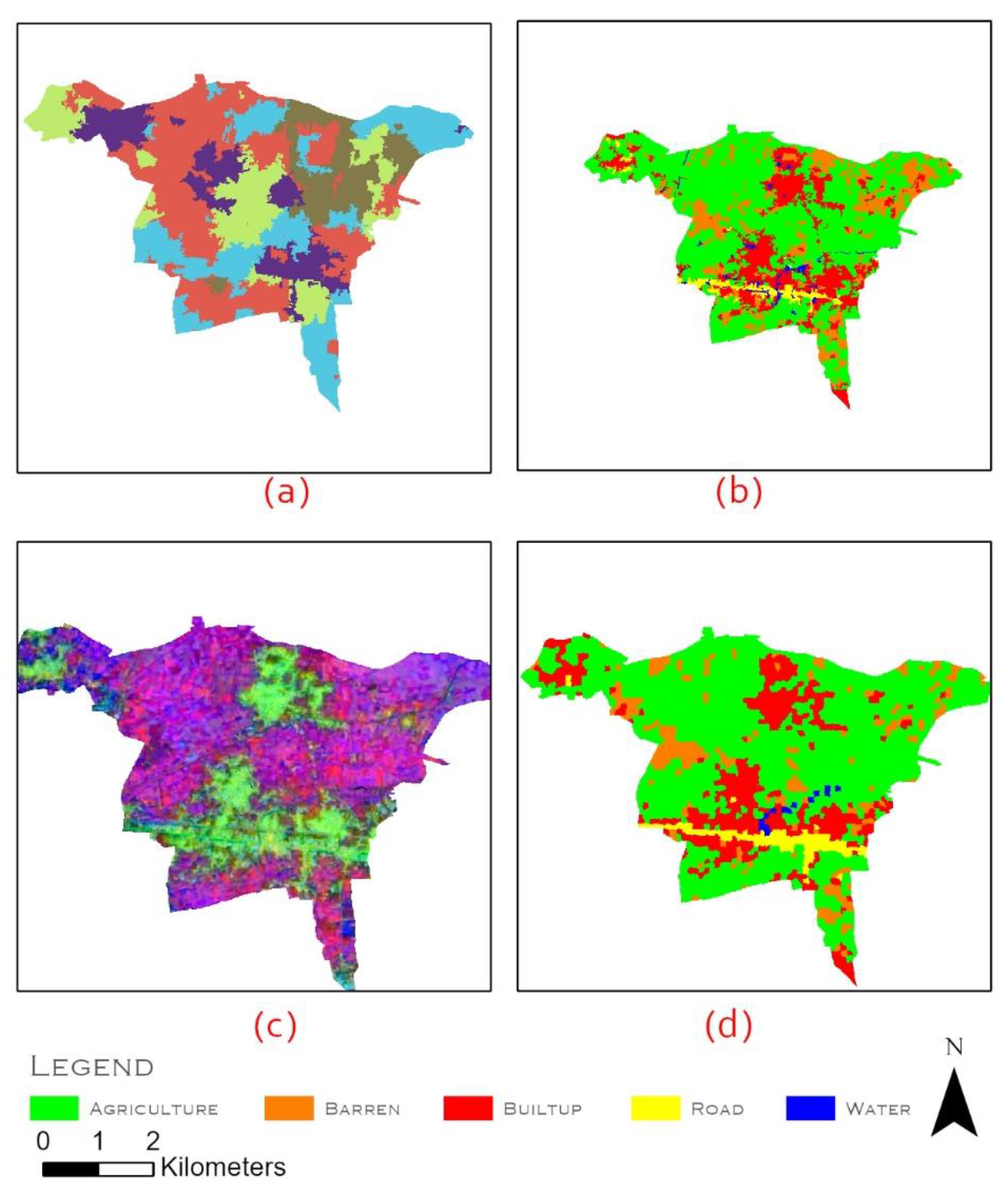
Table 1.
Land-use/land-cover (LULC) classes from the cadastral survey (1928–29).
| Class | Area (Hectare) | Parcel |
| Agriculture | 1725 | 6331 |
| Built up | 59 | 137 |
| Graveyard | 10 | 29 |
| Road/Streets | 90 | 193 |
| Stream | 46 | 320 |
| Grand Total | 1930 | 7010 |
Table 2.
Best value for SNIC seed and neighborhood size.
| Pipeline | Best OA | Best Kappa | Best Seed | Best Neighborhood | Trend Summary |
| OB-Spectral Indices | 0.95 | 0.92 | 10 | 128 | High accuracy at small seeds (fine segments); degradation as seed increases |
| OB-AlphaEarth Embeddings | 0.96 | 0.95 | 10 | 32 | Embeddings more stable, best performance at small seeds and moderate neighborhoods |
Table 3.
Summary of Overall Accuracy (OA), macro-averaged F1 score, and Kappa coefficient for all four classification pipelines
Table 3.
Summary of Overall Accuracy (OA), macro-averaged F1 score, and Kappa coefficient for all four classification pipelines
| Method | OA | F1 macro | Kappa |
| PBSI | 0.90 | 0.79 | 0.86 |
| PBAE | 0.95 | 0.81 | 0.92 |
| OBSI | 0.95 | 0.86 | 0.92 |
| OBAE | 0.96 | 0.89 | 0.95 |
Table 4.
Class-wise producer (PA) and user (UA) accuracies and F1 score for pixel-based classification pipelines.
Table 4.
Class-wise producer (PA) and user (UA) accuracies and F1 score for pixel-based classification pipelines.
| Classes | PBSI | PBAE | ||||
| UA (Precision) | PA (Recall) | F1 Score | UA (Precision) | PA (Recall) | F1 Score | |
| Agriculture | 0.92 | 0.96 | 0.94 | 0.96 | 0.99 | 0.97 |
| Barren | 0.92 | 0.89 | 0.90 | 0.93 | 0.94 | 0.94 |
| Built-up | 0.87 | 0.90 | 0.89 | 0.94 | 0.94 | 0.94 |
| Road | 0.80 | 0.60 | 0.69 | 0.98 | 0.94 | 0.96 |
| Water | 0.83 | 0.42 | 0.56 | 1.00 | 0.13 | 0.24 |
Table 5.
Class-wise producer (PA) and user (UA) accuracies for object-based classification pipelines.
Table 5.
Class-wise producer (PA) and user (UA) accuracies for object-based classification pipelines.
| Classes | OBSI | OBAE | ||||
| UA (Precision) | PA (Recall) | F1 Score | UA (Precision) | PA (Recall) | F1 Score | |
| Agriculture | 0.97 | 0.97 | 0.97 | 0.96 | 0.99 | 0.97 |
| Barren | 0.91 | 0.96 | 0.94 | 0.98 | 0.96 | 0.97 |
| Built-up | 0.95 | 0.91 | 0.93 | 0.96 | 0.94 | 0.95 |
| Road | 0.92 | 0.95 | 0.94 | 0.95 | 0.98 | 0.96 |
| Water | 0.80 | 0.40 | 0.53 | 0.75 | 0.50 | 0.60 |
Disclaimer/Publisher’s Note: The statements, opinions and data contained in all publications are solely those of the individual author(s) and contributor(s) and not of MDPI and/or the editor(s). MDPI and/or the editor(s) disclaim responsibility for any injury to people or property resulting from any ideas, methods, instructions or products referred to in the content. |
© 2025 by the authors. Licensee MDPI, Basel, Switzerland. This article is an open access article distributed under the terms and conditions of the Creative Commons Attribution (CC BY) license (http://creativecommons.org/licenses/by/4.0/).
Copyright: This open access article is published under a Creative Commons CC BY 4.0 license, which permit the free download, distribution, and reuse, provided that the author and preprint are cited in any reuse.


