
Submitted:
26 November 2025
Posted:
27 November 2025
You are already at the latest version
Abstract
Script-based computer-aided design (CAD) tools offer accessible, open, and highly customizable design environments, but their broader adoption is limited by the cognitive and computational difficulty of describing curved, irregular, or free-form geometries through code. Here, cognitive difficulty refers to challenges in curve interpretation, spatial reasoning, and mentally mapping geometric intent into parametric scripts, while computational difficulty relates to the mathematical effort, syntax precision, and debugging complexity required to generate valid geometries. Recent studies show that users frequently struggle with this combined burden, highlighting the need for more guided and intuitive workflows. This study presents a unified, open-source framework that addresses these challenges by enabling concept-to-CAD transformation through 2D point-based representations. The framework integrates an Interactive Point Cloud Modeling (IPCM) Layer with a set of modular systems for curve construction, point generation, transformation, and data formatting, together with script-based rendering functions for generating CAD geometry. These components allow users to generate geometrically valid digital models without navigating the heavy geometric calculations, strict syntax requirements, and debugging demands typical of script-based CAD workflows. Six structured case studies demonstrate the workflow across mechanical, artistic, and handcrafted forms, while additional examples highlight its applicability to cultural motif digitization, historical alphabet reconstruction, reverse engineering, and educational prototyping. These demonstrations also show that the framework can generate fabrication-ready outputs—including volumetric models, 2D profiles, and vector representations—highlighting its adaptability across diverse design and manufacturing contexts. All systems and functions are made publicly available, enabling the entire pipeline to be carried out using free and open-source tools. By providing a practical and reproducible basis for point-based modeling, the framework advances computational design practice and supports wider adoption of script-based CAD workflows.
Keywords:
design workflow
; digital fabrication
; open systems
; point cloud modeling
; script-based CAD
1. Introduction
Computer-Aided Design (CAD) has long been a cornerstone of modern engineering, manufacturing, and design education [1,2,3,4,5,6,7]. Traditional CAD systems such as AutoCAD®, SolidWorks®, CATIA®, Onshape®, and Fusion 360® have established powerful ecosystems for feature-based, GUI-driven modeling, enabling detailed product design, analysis, and simulation. However, these platforms often require substantial costs, computational resources, and specialized training, which can limit accessibility—particularly for small and medium-sized enterprises (SMEs), educational institutions, hobbyists, and individual innovators seeking lightweight or flexible design environments. At the same time, the expansion of digital fabrication technologies and open-source movements [8,9,10,11,12] has intensified the focus on personalized and one-of-a-kind product development [11,13,14,15,16,17]. Affordable 3D printing and small-scale manufacturing now allow individuals and small enterprises to produce customized products directly from digital designs. This growing culture of accessible and distributed fabrication has, in turn, heightened the demand for transparent, flexible, and customizable design tools, motivating a wide range of users—including students, hobbyists, educators, designers, and developers—to explore alternatives to conventional proprietary platforms.
Responding to this shift, a new paradigm of script-based and open-source CAD tools (e.g., OpenSCAD [18], CadQuery [19], and similar platforms) has emerged, reimagining the design process as a programmatic, generative, and collaborative activity. These tools allow users to define models through scripts (or code) rather than graphical manipulation, enabling parameterization, reproducibility, and integration with computational workflows. This code-driven design approach not only supports a high degree of automation and customization but also aligns with the growing movement toward open-source engineering and digital democratization in manufacturing. Several studies [20,21,22,23,24,25] illustrate this growing use of open-source, script-based CAD tools in practice. Additionally, the rise of generative AI and vibe coding (AI-assisted coding through prompting) has further strengthened the relevance of these script-based platforms—particularly in education, research, and rapid prototyping—by making code generation and model exploration more intuitive and collaborative. One may refer to the works in [15,17,23,26,27,28,29,30] to see how generative AI and vibe-coding approaches are increasingly being used to accelerate script-based CAD modeling.
Figure 1 illustrates the basic workflow differences between traditional CAD tools and script-based modeling environments. As seen in Figure 1(a), the traditional workflow (here, Onshape®) typically begins with a concept or a detailed 2D drawing containing dimensional information. The designer then opens a CAD application, selects an appropriate reference plane, and creates sketches using graphical tools such as lines, rectangles, circles, or ellipses. These sketches are transformed into three-dimensional forms through extrusion, revolution, or lofting operations, and additional features are generated by applying Boolean operations (union, difference, and intersection) through interface commands. In contrast, Figure 1(b) demonstrates how the same model can be created within a script-based CAD environment. On the left, an OpenSCAD script defines the same geometric entities and operations using parameterized code, while on the right, a CadQuery script performs equivalent modeling through a different syntax. In both cases, the designer constructs the object algorithmically, and rendering the script produces the resulting 3D model.
While Figure 1 illustrates the basic workflow of script-based CAD, it primarily represents simple geometric forms that can be described parametrically. In practice, however, many design tasks involve curved, irregular, or free-form geometries that are considerably more difficult to model through code. Figure 2 presents such cases, where Figure 2(a)–(c) correspond to dimensioned or technically defined parts such as contoured profiles and revolved surfaces, and Figure 2(d) depicts decorative or conceptual motifs derived from sketches or physical references. Even with dimensional data or reference drawings, recreating these shapes algorithmically requires detailed mathematical logic, curve formulation, and coordinate mapping. Traditional GUI-based CAD tools allow designers to sketch and refine parametric curves (Bezier, spline, B-spline, and NURBS) interactively with immediate visual feedback. In contrast, script-based tools demand explicit coding for each feature—often through lengthy, iterative processes that are difficult to adjust or debug. Even with vibe coding, achieving precise curvature or intricate form typically involves extensive trial and error. Although OpenSCAD and CadQuery include libraries for curve and surface generation, modeling complex free-form geometries remains a demanding and time-consuming task, posing a significant challenge to the wider adoption of script-based CAD in design, education, and manufacturing.
Recent studies reinforce the abovementioned observations. Gonzalez Avila et al. [31] identified that script-based CAD users face difficulties with spatial reasoning, script debugging, creating organic or curved shapes, and navigating complex script, collectively highlighting the limitations of current workflows. Follow-up research by the same group [25] further reports that parametric modeling in OpenSCAD requires substantial mathematical effort, often creating an unnecessary barrier for newcomers. Related work on augmented fabrication [32] also identifies challenges in transferring real-world geometry into digital models, particularly for novices working with free-form or physically constrained shapes. Collectively, these studies echo the practical issues described above and underscore the need for more accessible, guided workflows in script-based CAD. Motivated by these recurring difficulties, this study explores an intermediate, point-based mechanism designed to bridge conceptual intent with code-level geometry, offering a more transparent and manageable pathway for modeling complex forms.
Building on the above contemplation, this study proposes an open-source framework aiming to lower the difficulty of modeling irregular and free-form geometries in script-based environments. As part of this framework, a middle layer is introduced that enables users to interactively create, arrange, and export point clouds corresponding to the desired model or shape, which can then be utilized for rendering in script-based environments. This study also identifies the necessary functional requirements for developing the systems and functions related to the proposed framework, develops them (systems and functions), and demonstrates their applicability. For better understanding, the remainder of this article is organized as follows. Section 2 describes the proposed framework, Section 3 outlines the related systems, functions, and underlying requirements, Section 4 presents the systems and functions development, Section 5 demonstrates application examples, and Section 6 concludes the study with final remarks.
2. Proposed Framework
This section presents the conceptual basis of the proposed framework. In particular, Section 2.1 illustrates the difficulty in modeling irregular and free-form shapes in script-based environments through a simple example, highlighting the motivation behind seeking a more supportive approach. Section 2.2 then outlines the conceptual framework developed to address this difficulty.
2.1. Problem Framing and Motivation
Consider a user who wishes to model the wavy profile shown in Figure 3. Although simple in appearance, this geometry requires a smoothly varying outline that must be represented using a parametric curve. For clarity, this example is used to illustrate the steps involved when generating such a profile in script-based CAD environments.
Figure 4 shows the corresponding implementation in CadQuery (CQ). As seen in Figure 4 (see the code on the left side), the modeling process begins with a user-defined list of control-point coordinates. These points are then passed to a parametric curve function (here, spline) to construct the curved profile, after which the profile is closed and extruded into a solid model. The right side of Figure 4 visualizes the control points as yellow spheres, indicating that the resulting geometry directly reflects these specified coordinates. The full script used to reproduce this example is provided in Appendix A (Table A1).
Similarly, Figure 5 presents the same profile created in OpenSCAD. Since OpenSCAD does not include a native method for generating parametric curves, an interpolation function—in this example, a Catmull–Rom formulation—is implemented to compute intermediate points along the curve. A sampling loop then discretizes the curve into a polygon suitable for extrusion. As before, the control points shown on the right determine the overall shape, but the workflow requires additional steps for curve interpolation and sampling prior to forming the solid. The complete script for this case is also provided in Appendix A (Table A2).
These examples highlight several observations relevant to modeling irregular or free-form profiles in script-based environments:
- parametric curves are essential for representing smooth or irregular boundaries,
- some environments provide native functions (e.g., splines in CQ) while others require user-implemented formulations,
- control-point coordinates must either be manually specified or mathematically deduced—both of which require users to understand how point placement influences the curve,
- developing or adapting the mathematical logic for parametric curves becomes increasingly demanding when irregularities increase, and
- number of steps grows substantially as the geometry becomes less regular.
Although the example shape in Figure 3 is relatively simple, the process illustrated in Figure 4 and Figure 5 becomes considerably more demanding when handling shapes such as those shown earlier in Figure 2. In such cases, users must manage more control points, derive or approximate curve segments mathematically if needed, and implement additional logic to capture local irregularities. As the number or complexity of features increases, the cumulative mathematical and coding effort can become impractical—particularly for learners, occasional users, or those exploring script-based CAD for rapid prototyping.
The abovementioned observations motivate the development of a more supportive approach that facilitates the creation of irregular and free-form profiles while preserving compatibility with script-based CAD workflows. Section 2.2 introduces the conceptual framework designed to address this need.
2.2. Conceptual Framework
Design research widely recognizes that design activity unfolds through two fundamental but interdependent spaces: a conceptual space, where ideas, intentions, and possibilities are explored, and a formal or solution space, where these ideas are translated into concrete representations. This distinction is consistent with multiple established design theories. For example, the Double Diamond model [33] conceptualizes design as moving from problem exploration to solution definition, mirroring the transition from conceptual ideation to concrete design development. Likewise, Concept–Knowledge (C–K) Theory [34,35] explicitly separates the concept space (C), where ideas are expanded without predefined structure, from the knowledge space (K), where structured information and formal models are used to materialize concepts.
Across these frameworks, a common insight emerges: design involves moving back and forth between what can be characterized as a Concept Layer, where sketches, reference images, or ideas express intent, and a Design Layer, where this intent is translated into computable or manufacturable forms. However, when this transition is carried out in script-based CAD environments, a significant cognitive and computational burden arises [25,31,32]. Cognitively, users must map visual or intuitive geometric ideas into explicit coordinates, control points, and curve logic. Computationally, they must manage mathematical formulations, syntax precision, and debugging steps that increase disproportionately when geometries become irregular or free-form. As illustrated in Section 2.1, these combined challenges become increasingly severe when the geometry contains irregular or free-form features, making the concept-to-script translation step one of the major bottlenecks in contemporary code-driven CAD workflows.
To ease this transition, the proposed framework introduces an intermediate Interactive Point-Cloud Modeling (IPCM) Layer—inserted between the Concept Layer and the Script-Based Rendering Layer—providing an alternative to the traditional workflow that moves directly from concept to script (or code), as shown in Figure 6. In this layer, users interactively construct structured point clouds that reflect their visual understanding of the intended geometry. Instead of determining control-point coordinates through trial-and-error or writing interpolation logic manually, users manipulate points through intuitive interfaces. These control points are then evaluated using standard parametric curve formulations—such as Bézier curves, Bernstein polynomials, splines, or related approaches—to generate smooth profiles consistent with the user’s adjustments. As illustrated in Figure 6, the IPCM Layer is conceived as a set of supporting subsystems (System A, B, C,…) that collectively enable this process. The resulting point cloud sets are then supplied to the Script-Based Rendering Layer, where dedicated functions (Function A, B, C,…) use the points to construct the solid model or generate alternative formats as needed (such as SVG, DXF, STL, or OBJ).
To illustrate how the proposed workflow operates, Figure 7 presents a minimal end-to-end example using the same wavy profile introduced earlier (Figure 3). As seen in Figure 7, the wavy profile corresponds to the Concept Layer, where the desired outline is defined. Within the IPCM Layer, a structured point cloud representing this outline is generated interactively; only the resulting points are shown here for demonstration purposes, without system-level descriptions. These points are then passed to the Script-Based Rendering Layer, where a short OpenSCAD script constructs the solid model. This example highlights how the IPCM Layer mediates between conceptual intent and script-based rendering. It also demonstrates the merit of having such an intermediate layer, compared with the challenges observed in the traditional workflow—such as manually determining control-point coordinates, formulating parametric curves, implementing interpolation logic, and managing increasingly long scripts, as outlined in Section 2.1. By introducing an intermediate layer, the proposed framework provides a practical means of reducing this burden. Instead of relying on mathematical deduction or trial-and-error coding, users can generate geometry-ready point sets through intuitive manipulation.
It is worth mentioning that the idea of using human cognition to construct point clouds has precedent in earlier studies [35,36,37], where point sets were generated analytically through recursive or user-defined algorithms. These works demonstrate that if humans can perceive sub-shapes or components within a target object, they can also contribute to constructing its digital representation. However, these studies focus on specific demonstration cases and do not serve as general-purpose workflows. Moreover, they do not articulate system-level definitions, requirements, or provide modular developments that could support broader reuse or extension. As a result, they rely on manual parameter adjustment and example-specific logic, and the reconstruction stage frequently depended on proprietary CAD tools. While these contributions established the conceptual possibility of cognition-guided point construction, their workflows were not structured in a way that could be readily adapted or extended to broader applications. The present framework builds on this foundational insight by operationalizing it into a reproducible, open-source workflow that generalizes the idea and makes it applicable across a wider range of design contexts. Rather than an ad hoc or example-specific process, the IPCM Layer organizes point-cloud creation into a structured and flexible workflow that complements script-based modeling while reducing the burden associated with low-level geometric definition.
Nevertheless, practical questions emerge: What systems and minimum functionalities are required for the IPCM Layer to reliably support the modeling of irregular or free-form geometries, and what functions are necessary within the Rendering Layer to materialize the proposed framework? The following section addresses these questions.
3. Systems and Requirements
As outlined in Section 2, this section presents the systems, requirements, and functions associated with the proposed framework. For clarity, Section 3.1 and 3.2 describe these elements for the IPCM and Rendering Layers, respectively.
3.1. IPCM Layer
As established in Section 2, the IPCM Layer forms an intermediate stage, enabling a structured transition from conceptual intent to script-based rendering. To make this possible, the IPCM Layer must consist of several systems that collectively support the creation, transformation, and preparation of point-cloud data required for use in script-based CAD environments. The systems and their purposes are described below.
3.1.1. System A—Generating Point Cloud for Irregular Profiles
Because irregular and free-form geometries are a primary focus of the proposed framework, the IPCM Layer must include a system that allows users to construct such profiles interactively. Users place and adjust control points through a visual interface, and the system evaluates these points using standard parametric curve formulations to generate a structured point-cloud representation of the intended outline.
Examples in Figure 2 illustrate the relevance of this capability. The curved boundary in Figure 2(a), the varying body curvature of the vase in Figure 2(b), the handle profile in Figure 2(c), and the organic outlines in Figure 2(d) all contain irregularities that require curve evaluation based on user-defined control points. This system provides the functionality by forming continuous point sets aligned with the user’s visual interpretation of such features.
3.1.2. System B—Generating Point Cloud for Geometric Elements
In addition to irregular profiles, many objects include regular geometric features such as circle, ellipse, and rectangle segments. Although script-based CAD environments typically provide native primitives for modeling these features, the IPCM Layer must include a system for generating point clouds corresponding to such geometric elements when needed. This enables users to maintain a unified point-cloud workflow regardless of whether a feature is free-form or geometric.
3.1.3. System C—Transforming Generated Point Clouds
Many design tasks require adjusting the spatial position, size, or orientation of a generated point cloud before it can be used meaningfully. For example, translation is needed to reposition a point set relative to a reference frame or rotation axis; scaling allows dimensional adjustment when the canvas-generated points must match real sizes; mirroring enables left–right or top–bottom reflection when a full shape can be constructed from a half-shape; and rotation supports generating repeated or radially arranged features. Collectively, these transformations allow a single point set to be repurposed, extended, or spatially coordinated without redrawing it—making System C essential for preparing point clouds for downstream rendering.
In the context of the examples shown in Figure 2, these needs appear naturally. For Figure 2(a–c), which include profiles with explicit dimensions, scaling ensures that the sampled points conform to the required real-world sizes. For Figure 2(b–c), which represent features formed by revolution, translation may be required to align the profile curve with the intended axis before rotation. For Figure 2(a) and Figure 2(d), repeated or radially arranged elements—such as contour segments or petal-like motifs—can be produced from a single representative segment through rotation. System C provides these operations in an integrated form, enabling users to construct complete geometries from minimal initial input while maintaining spatial correctness across all transformed point sets.
3.1.4. System D—Cleaning and Sequencing of Point Clouds
Many rendering operations require point sets to follow a consistent ordering so that they form a continuous outline or boundary. For this reason, the IPCM Layer requires a system dedicated to cleaning and sequencing point clouds before they are passed to the rendering stage.
When points are generated across multiple curve segments or transformed through operations such as rotation, mirroring, or scaling (as mentioned in Section 3.1.3), the resulting coordinates may not follow a proper traversal order or may contain duplicates. System D resolves such issues by producing an ordered, duplication-free point set that conforms to the requirements of rendering functions expecting structured and sequential point arrays.
3.1.5. System E—Formatting of Point Clouds for Rendering Environments
Because a shape generated in the IPCM Layer is ultimately represented as a sequence of points (xi,yi) for i = 1,2,…, the point set must be exported in a structure compatible with the target rendering environment. However, script-based CAD platforms differ in how such point data must be written. For example, OpenSCAD expects point arrays in the form [[x1, y1], [x2, y2], …], whereas CadQuery typically uses Python tuples such as [(x1, y1), (x2, y2), …]. This system ensures that the point data generated in the IPCM Layer can be inspected and formatted according to these environment-specific conventions, enabling seamless transfer to the Script-Based Rendering Layer.
3.1.6. Systems Requirements
The discussions above distill into a set of functional requirements that must be ensured when developing the systems. Table 1 outlines these requirements and indicates how they correspond to each system within the IPCM Layer.
As shown in Table 1, System A—responsible for generating point clouds for irregular and free-form profiles—must provide a visual user interface equipped with both direct and indirect manipulation capabilities for placing and adjusting control points. Because users typically rely on a reference sketch or image when tracing free-form outlines, System A must also support data importing, allowing a background or overlay image to be loaded onto the canvas for guided point placement. It must also evaluate these points using standard parametric curve formulations. In many cases, however, a single curve is insufficient to represent an entire outline. The system must therefore support piecewise construction, allowing the user to divide the shape into multiple curve segments based on visual cognition. For example, the bird motif in Figure 2(d) contains several distinct curvature regions—such as the head arc, wing contour, and tail bend—that cannot be captured adequately by a single parametric curve. Each segment may also require a different sampling density depending on its geometric complexity: small or simple features may need only sparse sampling, while detailed regions require a higher density of points. Thus, the system must support piecewise point sampling as well. In addition, System A must manage continuity, ensuring that adjacent segments connect meaningfully when a continuous outline is intended or remain independent when discontinuity is appropriate. Finally, System A must allow the resulting point sets to be exported for subsequent use.
As shown in Table 1, System B—responsible for generating point clouds for geometric elements—must provide a visual interface equipped with both direct and indirect manipulation capabilities that allows users to specify regular primitives through simple selections or minimal input parameters. As geometric primitives are often traced or aligned relative to a reference sketch, System B must also support data importing, enabling users to load a background or overlay image on the canvas for guided placement and adjustment. Behind the interface, the system must incorporate the mathematical formulations needed to compute point clouds for common geometric features such as circles, arcs, ellipses, and rectangles. For example, when a user selects a circle, the system must automatically evaluate standard parametric equations (e.g., , ) using either user-specified parameters or a small number of guiding points, such as three points on the circumference. The same principle applies to ellipses, partial arcs, and other primitives. This ensures that geometric features—such as the circular regions in Figure 2(a) or the eye in Figure 2(d)—can be represented with consistent accuracy within the point-cloud workflow. As with other systems in the IPCM Layer, System B must support exporting the generated point sets for subsequent use.
As shown in Table 1, System C—responsible for transforming generated point clouds—must provide an interface for importing and transforming points. Behind this interface, the system must implement the mathematical operations required to perform geometric transformations such as translation, rotation, mirroring, and scaling. These transformations rely on standard linear-algebra formulations (e.g., rotation matrices, reflection matrices, and translation vectors), which the system must apply automatically when the user triggers a transformation command. This capability allows users to construct repeated or symmetric features efficiently—for instance, replicating a single petal-shaped point cloud to form the radial arrangement suggested in Figure 2(d), or creating mirrored curvature patterns such as those indicated in Figure 2(a). The transformed point sets must remain exportable for subsequent use.
As shown in Table 1, System D—responsible for cleaning and sequencing point clouds—must ensure that the generated or transformed points follow a coherent traversal order suitable for downstream rendering. When point sets are created piecewise, merged from multiple segments, or manipulated through operations such as rotation or mirroring, their natural sequence is often disrupted. The system must therefore incorporate mechanisms for importing the generated point sets, and for determining and adjusting their order using simple but essential algorithms such as nearest-neighbor traversal, angular sorting, or user-guided re-indexing. A visual interface must allow the user to inspect the current order and make corrections when necessary, ensuring that the final sequence forms a meaningful boundary or path for reconstruction. This requirement becomes particularly important in scenarios where multiple features are combined, such as stitched curve segments or mirrored petals from Figure 2(d). As with the other IPCM systems, the ordered point sets must be exportable for subsequent use.
Finally, as shown in Table 1, System E must ensure that the generated point sets can be imported, inspected, and written in the appropriate format for the target rendering platform. To support this, the system should provide simple inspection utilities—such as tabular views or basic plots—that allow users to verify point correctness before export. System E may also be realized through common spreadsheet editors (e.g., LibreOffice Calc® or Google Sheets®), enabling users to refine, manually transform, or adjust point values when needed. By handling import, verification, manual transformation, and standardized formatting, System E ensures seamless transfer of point-cloud data to the Script-Based Rendering Layer.
3.2. Script-Based Rendering Layer
The Rendering Layer receives structured point-cloud data from the IPCM Layer and must provide functions that directly operate on these points to produce the intended output. Because users may require either 2D or 3D representations, these functions must be designed flexibly. For outlines, the functions must be able to construct paths from the supplied points regardless of whether the sequence is open or closed. In contrast, the generation of 2D surfaces requires a closed point sequence that defines an enclosed region; an open sequence cannot form a surface. The Rendering Layer must therefore allow users to specify whether a given point set should be treated as an open path, a closed boundary, or a surface-generating loop, depending on design intent.
To support further modeling, functions must also extend from 2D to 3D. A closed surface may be extruded into a solid, and users must be able to control extrusion direction and magnitude directly from the point-defined geometry. Likewise, any point-derived shape—whether a path, surface, or solid—must be transformable through translation, rotation, mirroring, and scaling. When multiple solids are created, the Rendering Layer must support Boolean operations (union, difference, intersection) so that users can combine or modify point-derived models without reverting to geometric primitives.
The Rendering Layer must also include functions for exporting the resulting geometry in various formats. For instance, paths may be exported as SVG or DXF, while solids may be exported as STL or OBJ. These capabilities allow point-based designs to be used directly for visualization, 3D printing, or downstream CAD operations.
Finally, the Rendering Layer must provide functions that can directly utilize the point sets generated in the IPCM Layer. When native functions already support the abovementioned operations (such as path creation, extrusion, Boolean operations, or export) without additional burden on the user, they can be used as-is. However, when native functions cannot operate on point clouds in the required manner, the Rendering Layer must include a set of custom functions designed specifically to interpret and reconstruct models from the points. These custom functions may rely on fully custom logic or combine native commands with additional procedures, but in all cases they must be exposed to the user as accessible templates—ensuring that point-based workflows require minimal input and remain consistent with the overarching goal of lowering the entry barrier for script-based modeling.
4. Developing Systems and Functions
This section presents the developed systems and functions corresponding to the definitions and requirements outlined in Section 3. For clarity, Section 4.1 details the development of the systems that constitute the IPCM Layer, and Section 4.2 presents the functions developed for the Script-Based Rendering Layer.
4.1. Developing Systems for IPCM Layer
This subsection describes the tools, techniques, and implementation approaches used to realize each system in the IPCM Layer, and provides flowcharts that illustrate how the systems operate in practice. The underlying mathematical formulations are summarized in the relevant appendices, while full source code and web-based implementations are made accessible through the provided URLs.
4.1.1. System A—Generating Point Cloud for Irregular Profiles
System A is realized through two algorithmic implementations, referred to as System A1 and System A2. Both implementations fulfill the same role as defined by the requirements in Section 3. System A1 is built on a Bézier–Bernstein polynomial formulation [38,39], where both the curve-evaluation logic (i.e., computing the continuous curve from a set of control points) and the point-sampling procedure (i.e., generating discrete points along that curve) are implemented directly in JavaScript (JS). System A2, by contrast, employs the spline-based curve generation functions of the open-source D3.js library (version 6.7.0) [40,41,42], combined with custom JS routines for extracting sampled points from the rendered spline curve. The inclusion of two implementations reflects the fact that there are multiple valid parametric curve formulations, each offering different modeling characteristics: Bézier curves tend to exhibit global influence from individual control-point adjustments, while spline-based curves offer more localized control and greater stability for complex outlines. As such, System A is designed to accommodate multiple curve formulations, with the flexibility to incorporate additional algorithms in future extensions of the framework.
Regardless of whether A1 or A2 is used, System A provides the same user-level capabilities. Each implementation offers a canvas on which the user may load a reference image (if needed) or work within a blank workspace. Through a set of buttons, input boxes, and context-dependent prompts, the user can specify the number of curve segments (pieces), interact with a canvas, place and drag control points for each segment on the canvas, assign the number of sampled points per segment, indicate whether successive segments should be continuous or independent, and visualize the resulting sampled points along the curve. Note that, here, continuity refers to C0 continuity. (C0 continuity is a property where adjacent curves are connected at their joints without any gaps, meaning they share the same endpoints. For two curves to have C0 continuity, the end of one curve must be exactly the same point as the beginning of the next curve.). Once the user is satisfied, the combined point set can be exported in CSV format. In this way, both implementations of System A satisfy the functional requirements outlined in Table 1 in Section 3.
Figure 8 shows the workflow of System A. The user begins by choosing either System A1 or System A2. Either system provides an 800 × 600 (width × height) canvas, where a reference image may be loaded or the user may work on the blank canvas. The user then specifies how many curve segments will be created and begins working on the first one. For each segment, the user places control points directly on the canvas and may drag them to refine the intended shape; the system continuously redraws the curve as these points are adjusted. Once the control points are in place, the user sets the number of points to be sampled from that segment, and the system automatically generates the sampled points along the drawn curve. Before moving to the next segment, the user may choose whether the new segment should start from the last point of the previous one (ensuring continuity) or begin independently. Each completed segment’s points are then stored, and this process repeats until all specified segments are defined. When the final segment is finished, the system merges all segments, allows the user to visualize the combined point set on the canvas, and finally exports the full collection of labeled control and sampled points as a CSV file for downstream use.
Table B1 in Appendix B summarizes the mathematical formulations associated with the abovementioned workflow, particularly the formulations used for curve evaluation, point sampling, and the construction of the final point-cloud set from the defined segments, corresponding control points, and number of points to be sampled, when Bézier–Bernstein polynomial formulation (System A1) is considered. Similarly, Table B2 in Appendix B summarizes the same when spline-based formulation (System A2) is considered. It is worth mentioning that the algorithms shown in Table B1 and Table B2 differ specifically in the steps related to curve formulation and point sampling. In Table B1, the curve formulation is implemented directly within the system, providing access to the parametric curve and enabling sampled points to be computed immediately from its mathematical expression. But in Table B2, a spline implementation from D3.js is adopted, which does not expose the underlying curve coordinates and instead outputs an SVG path. Consequently, additional JS routine is developed to interpret the SVG path geometry and extract the required sampled points.
4.1.2. System B—Generating Point Cloud for Geometric Elements
Like System A, System B is implemented using custom JS routines to generate point clouds for geometric elements such as circles, arcs, ellipses, and polygons. As outlined in Section 3, although script-based CAD environments already provide native commands for constructing these primitives, System B serves as a complementary mechanism that enables users to create point-based representations of such shapes in parallel with the irregular profiles produced by System A. In this way, both geometric and free-form components are handled within the same IPCM Layer.
Figure 9 shows the workflow of System B. The system provides the same 800 × 600 canvas used in System A, where the user may load an optional reference image or work directly on a blank workspace. As seen in Figure 9, the user begins by selecting a geometric primitive from a dropdown menu—currently supporting circle, ellipse, arc, major arc, and polygons. For primitives that require geometric computation (e.g., circle, ellipse, arc, major arc), the user must place a minimum set of reference points on the canvas. For example, a circle requires three points on its circumference, and an arc requires three points defining its curvature. The dropdown menu indicates both the number and the order in which these points must be defined. Once the required points are placed, the system computes the corresponding curve and generates a point-cloud representation using its internal sampling routine. For polygonal shapes, the process is entirely point-based: the user simply clicks to specify the vertices, and the system connects them directly without further computation. As seen in Figure 9, the resulting point cloud can then be visualized and exported as a CSV file.
Table C1 in Appendix C summarizes the formulations used in System B for modeling the available geometric shapes as point clouds. As seen in Table C1, each primitive is described in terms of its required user inputs (e.g., number and type of reference points), the logical steps used to interpret those inputs in the computation, and the resulting point sets that are generated on the canvas.
4.1.3. System C—Transforming Generated Point Clouds
Like Systems A and B, System C is also built on custom JavaScript routines to perform geometric transformations on point clouds generated by the previous systems. It provides operations such as translation, mirroring, rotation, scaling, and sampling, allowing users to modify a point cloud directly within the IPCM Layer. As outlined in Section 3, such transformations are often necessary when multiple point-cloud sets must be created from a single base geometry—for example, in cases where symmetric or repeated features share an identical underlying shape.
Figure 10 shows the workflow of System C. As seen in the figure, the user begins by loading a point cloud in a predefined CSV format (X, Y). The system visualizes the uploaded data using open source Plotly.js library (version 2.24.1) [43], supporting three plotting styles—scatter, line, and line-with-markers—to assist the user in examining the geometry. After visualization, the user selects a transformation type from a horizontal tabbed menu. The currently supported operations include translation, mirroring, rotation, scaling, and sampling, each implemented through custom JS routines. In particular, Translation shifts every point in the cloud by a user-specified offset in the x and y directions. Mirroring reflects the point cloud across either the x-axis, y-axis, or an arbitrary user-defined vertical or horizontal line. Rotation turns the entire set of points about a chosen reference point—either the origin (0,0) or a user-defined coordinate—and may be applied clockwise or counter-clockwise. Scaling expands or contracts the points. Two types of scaling are supported: (1) global scaling, which multiplies every coordinate by a user-defined factor relative to the global origin, and (2) range-based scaling, which remaps the x- or y-coordinates so that the point cloud fits a new user-specified interval. Sampling reduces the number of points by extracting every k-th point from the current set, enabling point-density control. Notably, each newly applied transformation operates on the most recently generated point set, enabling chained operations that progressively build complex variations from a single base geometry. This capability is particularly useful for creating repeated or symmetric elements—for example, rotating a point cloud multiple times to produce evenly spaced radial features. A reset option is also available in the interface to restore the original loaded point cloud whenever needed. All generated sets can also be exported together as a CSV file for downstream use.
Table D1 in Appendix D summarizes the mathematical formulations underlying the above transformations. Let the loaded or current point cloud be denoted by L ={Li = (xi, yi) | i = 0,1,…,N-1}. Each transformation maps L to a new point set T = {Ti = (x’i, y’i)}. Table D1 lists the required user inputs and the corresponding computational rules used to obtain T from L.
4.1.4. System D—Cleaning and Sequencing of Point Clouds
System D extends the IPCM Layer by providing essential preprocessing operations for the generated point-cloud data. As noted in Section 3, such data may contain duplicate coordinates or lack a meaningful sequential order, further leading to inconsistencies during downstream modeling or rendering. To support this requirement, System D is implemented in Python programming language (version 3.10) [44] using libraries such as Tkinter, Pandas (version 2.3.3) [45], SciPy (version 1.15.3) [46], and Matplotlib (version 3.10.7) [47]. A nearest-neighbor–based method is currently employed to establish point order, while the framework is designed to accommodate additional sorting algorithms in future updates. This way, System D enables users to prepare clean, structured, and reliable datasets within the IPCM Layer before rendering when needed.
Figure 11 shows the workflow of System D. As seen in Figure 11, the process begins by loading point cloud data in a predefined CSV format (X, Y, Z), where the system reads the file using Pandas and normalizes the required columns so that X and Y are always present and Z is added as 0 if unavailable. Duplicate points are then identified by checking repeated (X, Y) pairs, and these duplicates are logged in the text area and removed to form a cleaned dataset. From this clean set, the system constructs an ordered traversal of the points using a nearest-neighbor strategy implemented with SciPy’s KDTree. The process begins by identifying the leftmost point in the dataset—that is, the point with the smallest X-coordinate—which becomes the starting point of the sequence. The cleaned point set is then indexed in a KDTree, allowing the system to efficiently query the closest unvisited point at each step. At every iteration, the algorithm takes the current point, retrieves its neighbors sorted by distance, and selects the nearest one that has not yet been visited. This procedure continues until every point in the cleaned dataset has been assigned a position in the sequence. If the user enables the close loop option, the algorithm then appends the starting point to the end of the sequence, forming a closed cycle suitable for applications that require a continuous loop. Throughout this process, the interface provides visual feedback by plotting the original, cleaned, and sorted point sets using Matplotlib and by writing diagnostic messages—such as counts, indices, and mappings between original and sorted positions—into the log panel. Finally, the system allows the user to export the original, cleaned, and sorted datasets as separate CSV files, ensuring that each stage of the preprocessing pipeline remains accessible for downstream use.
Table E1 in Appendix E summarizes the mathematical formulations corresponding to the above operations. Let the loaded point cloud be denoted by L ={Li = (xi, yi) | i = 0,1,…,N-1}, which may contain duplicated coordinates or lack a meaningful sequential structure. Each operation transforms L into an intermediate or final dataset, such as the cleaned set C or the ordered set T, according to the computational rules listed in Table E1.
4.1.5. System E—Formatting of Point Clouds for Rendering Environments
System E, which provides a lightweight formatting environment within the IPCM Layer for preparing point-cloud data for downstream CAD workflows, is implemented using custom JavaScript routines that integrate open source JS libraries: Plotly.js (version 2.24.1) [43] for plotting and visualization, jSpreadsheet CE or formerly jExcel.js (version 4.15.0) [48] for spreadsheet-style data editing, and jSuites.js (version 4.17.5) [49] for UI components and auxiliary interface behaviors. As outlined in Section 3, point-cloud datasets often need to be inspected, verified, and reformatted according to the requirements of the environment in which they will ultimately be used. System E offers this capability within the IPCM Layer.
Figure 12 shows the workflow of System E. The process begins by loading point-cloud data, either from a CSV file or by pasting the raw coordinates directly into the interface. The data are then visualized, allowing the user to verify the overall structure and distribution of points before proceeding. If necessary, the dataset can be inspected or modified in the spreadsheet panel, where all numeric values are displayed in an editable tabular format. Once the dataset is finalized, System E converts the points into the syntax required by downstream CAD environments such as CQ or OpenSCAD. The formatted output can then be exported as a text file or copied directly from the workspace for immediate use.
Note that although a built-in spreadsheet editor is provided to support a unified user experience, equivalent functionality can also be achieved using established open-source tools such as LibreOffice Calc® or Google Sheets®. The integrated editor remains under active development and is not yet intended to replace such full-featured spreadsheet solutions.
4.2. Developing Functions for Rendering Layer
As described in Section 3, the Script-Based Rendering Layer receives structured point-cloud data from the IPCM Layer and convert these points into usable geometric entities. In standard script-based environments such as OpenSCAD or CQ, powerful native operations already exist. For instance, revolving a 2D sectional profile to generate a solid model of vase or cup, or performing Boolean operations between solids. However, such operations assume that the user already possesses a well-defined geometric primitive or curve representation. When only an arbitrary sequence of points is available, these native tools cannot operate directly, creating a gap between point-based modeling and conventional solid-modeling workflows. To address this, the Rendering Layer must provide a minimal set of custom functions capable of interpreting point sequences as paths or boundaries so that users can obtain an immediate renderable shape before applying higher-level modeling operations. In the present work, OpenSCAD (development snapshot, version 2025.07.02 (git 3880cb321)) [18] is adopted as the primary rendering environment, ensuring that point-derived geometries can be visualized and manipulated as early as possible. Accordingly, a small collection of custom functions has been developed to make these point sets directly meaningful in OpenSCAD while still remaining compatible with its native modeling operations; equivalent implementations for CadQuery can be realized in the same manner when needed.
Table F1 in Appendix F summarizes the developed functions for OpenSCAD, listing their syntax, purpose, and required input arguments. These functions together form the basic rendering toolkit needed to make point-cloud data immediately usable within the Script-Based Rendering Layer. As outlined in table F1, the ‘close_path’ function converts an open sequence of points into a closed loop when a boundary or enclosed surface is required. The ‘show_points’ function provides a mechanism for visually inspecting the point distribution by drawing spheres at each coordinate. For surface-based representations, the ‘create_polygon’ function interprets an ordered point set as a 2D region. The ‘extrude_polygon’ function extends this region into a 3D solid through linear extrusion. For path-based representations, the ‘create_2d_path’ function constructs a continuous outline by sweeping circular or square cross-sections along the supplied points using hulling operations. Its 3D counterpart, the ‘extrude_2d_path’ function extrudes the generated 2D path vertically to produce tubular or block-like solids. Collectively, these functions provide a minimal yet complete set through which point-defined geometries can be rendered in OpenSCAD and then further refined using its native operations.
Nevertheless, all the developed systems have also been implemented as independent web-based tools, accessible at the portal: https://commons-repo.github.io/002-research/. Figure 13 shows a screenprint of the portal’s index page, where all the systems (Systems A (A1 and A2), B, C, D, and E, corresponding to Section 4.1.1–4.1.5) are hosted. As seen in Figure 13, each system can be accessed directly by selecting its panel, while the documentation link (shown at the bottom of the portal page) provides access to all supporting files and examples. These supporting materials include the system-wise user guides, illustrative examples, the OpenSCAD template file for the rendering functions (corresponding to Section 4.2), and its corresponding user guide, allowing users to understand and reproduce the complete set of workflows. Note that maintaining the systems as independent tools within this portal is a deliberate design choice: it allows each system to evolve modularly, simplifies experimentation, and enables iterative upgrades without interfering with rest of the components.
Importantly, all the developed systems operate entirely on the client side and do not store or transmit any user data. Point-cloud files, images, and design inputs remain within the user’s local environment, ensuring that proprietary concepts or geometry are never uploaded or retained externally. Yet, for offline use, the complete repository can be downloaded from https://github.com/commons-repo/002-research.git (or via the GitHub CLI: gh repo clone commons-repo/002-research). Once downloaded, the systems can be run locally by simply opening the included index.html file. All JavaScript (JS) routines developed for the systems—including the logic corresponding to the workflows, formulations, and algorithms described earlier—are fully contained in the repository to support transparency, reuse, and further extension. The repository also includes the OpenSCAD template file and all supporting materials referenced above.
Supporting materials, especially the system-wise user guides, are also included as supplementary documents to this manuscript. These guides provide the operational details that cannot be accommodated within the main text. These help users walk through each system step by step. To ensure continuity, a consistent set of example datasets is used across all guides and in the rendering-layer demonstrations, enabling readers to follow the complete workflow and reproduce the results in their own environment.
5. Application
This section demonstrates how the proposed framework operates in practice by applying it to the representative shapes introduced earlier in Figure 2. The focus is on showing how the developed systems and rendering functions collectively enable users to construct solid models. Operational details—such as how individual systems are used, how points are placed or adjusted, or how transformations are executed—are not repeated here. These aspects are already addressed in Section 4, where each system was presented with workflow diagrams, algorithmic formulations, and accompanying documentation. Accordingly, this section concentrates only on the integrated use of the developed systems and functions.
5.1. Case 1
Recall the concept shown in Figure 2(a). Figure 14 illustrates how the developed systems are used to generate the corresponding point clouds in the IPCM Layer. As seen in Figure 14, the process begins with System A (A1), where the outline of a single tooth is constructed as two curve segments that share a common endpoint to maintain continuity; the distinction between these segments is indicated by the black and orange points in the figure. The sampled points from both segments collectively form the base geometry for one repeating tooth profile. System B is then used to generate the point cloud for the circular inner region, and in addition to producing the sampled points for this region, it provides the center coordinates required for subsequent operations. Using this center information, the tooth profile is supplied to System C, which performs rotational replication to generate the complete set of teeth. Because the concept contains 36 teeth, System C rotates the base profile in increments of 10 degrees, producing 35 additional copies. As seen in Figure 14, the resulting rotated points are then merged with the circular point set obtained from System B. Although these merged points preserve proportional relationships, they still reflect the coordinate range of the working canvas (800 × 600). To recover the intended scale of the concept—specifically, an outer radius of 125 units—the combined dataset is processed again in System C using its scaling function: the X-axis range is remapped to [–125, 125], and the Y-coordinates are uniformly scaled to maintain proportionality. The purple points in Figure 14 show the scaled result. With scaling complete, the combined dataset is transferred to System E, where the merged points are separated into two distinct sets—one for the outer teeth and one for the inner circle—using the spreadsheet editor. Finally, System E formats each set into OpenSCAD-compatible point lists, producing the two structured arrays (points1 and points2) that serve as inputs for the rendering stage.
Figure 15 shows the rendering stage for the above. As seen in Figure 15, the two point sets (points1 and points2) prepared above are first inserted into an OpenSCAD script. The script begins by including the developed template file using the ‘include <openscad_template.scad>’ command. In this script, the point lists are defined and then passed to the template’s custom functions. Each set of points is first processed with ‘close_path’ to ensure a closed boundary, after which the resulting paths are supplied to ‘extrude_polygon’ to generate the corresponding solids. Following this, OpenSCAD’s native ‘difference’ operation is applied to combine these solids and produce the final blade geometry shown in Figure 15. Once the model is constructed, it can then be exported in standard CAD formats such as STL, OBJ, or STEP for downstream use.
5.2. Case 2
Recall the concept shown in Figure 2(b), which provides a sectional representation of a vase profile. Figure 16 illustrates how the developed systems are used to generate the corresponding point cloud in the IPCM Layer. As seen in Figure 16, the user first reconstructs the sectional curve by dividing it into 21 segments, each handled in System A (A1), where continuity is maintained between successive segments but not between the first and twenty-first; this is shown through alternating black and orange point sets that mark segment boundaries. The sampled points from all 21 segments are then combined to form the complete cross-sectional curve. This collective point set is next supplied to System C for scaling. In contrast to the previous example, scaling is performed along the Y-axis because the concept in Figure 2(b) specifies a total height of 160 units; accordingly, the Y-range is remapped to [0, 160], and the X-coordinates are scaled uniformly to preserve proportionality. The resulting scaled curve is shown in purple in Figure 16. Since this point set represents a 2D cross-sectional profile, it must be aligned with the rotation axis before being revolved into a solid. For this purpose, the scaled points are input again into System C, where the entire set is translated horizontally by an offset of –353.83513 (determined from the plotted coordinates) to align the profile with the vertical axis through the origin. The translated curve is shown again in Figure 16. Finally, this aligned point set is transferred to System E, where it is formatted into an OpenSCAD-compatible point list named ‘points’, which is used directly in the rendering stage.
Figure 17 shows the rendering stage for the above. As seen in Figure 17, the point set (‘points’) prepared above is inserted into an OpenSCAD script, which—similar to the previous example—includes the developed template file and calls its custom functions. In this script, the point list ‘points’ is defined and passed step-by-step through the template and native functions. First, the points are processed with ‘close_path’ to convert the sampled section into a closed boundary. Next, this closed boundary is supplied to ‘create_polygon’ for generating the corresponding 2D region. Finally, this region is placed inside a native ‘rotate_extrude’ block, which sweeps the profile around the vertical axis to produce the complete vase geometry shown in Figure 17.Once the solid is obtained, it can be exported in standard CAD formats such as STL, OBJ, or STEP for downstream use.
5.3. Case 3
Recall the concept shown in Figure 2(c). Figure 18 illustrates how the developed systems are used to generate the point clouds for both the cup body and the handle. As seen in Figure 18, the user first constructs these two components separately in System A (A1). The body is divided into seven curve segments and the handle into five, with continuity maintained between successive segments but not between the first and last—an arrangement indicated by alternating black and orange point sets in the figure. The sampled points from the seven body segments are combined to form one collective set, while the five handle segments form another. These two sets are then appended to create a single combined dataset, which is supplied to System C for scaling. Since the concept specifies an overall height of 33 units, scaling is applied along the Y-axis by remapping the Y-range to [0, 33] while uniformly adjusting the X-coordinates to preserve proportionality. The scaled result is shown in purple in Figure 18. This scaled dataset is then processed again in System C to align the body profile with the vertical axis for subsequent revolved solid generation. For this, the entire set is translated horizontally by –348.32001, as determined directly from the plotted coordinates. The translated points are also shown in Figure 18. Finally, this combined dataset is transferred to System E, where it is decomposed back into two separate sets—one for the body and one for the handle—and each is formatted as an OpenSCAD-compatible point list (points1 and points2) for the rendering stage.
Figure 19 shows the rendering stage for the above. As seen in Figure 19, the two point sets (points1 and points2) prepared above are inserted into an OpenSCAD script that begins, as before, by including the developed template file. In this script, the first set, points1, represents the cup body and is processed step-by-step: the points are first passed to ‘close_path’ to form a closed profile, after which the resulting boundary is supplied to ‘create_polygon’ inside a ‘rotate_extrude’ block to generate the revolved outer geometry of the cup. The handle uses the second point set, points2, which is likewise closed using ‘close_path’ and then converted into a 2D region through ‘create_polygon’. This region is extruded using ‘extrude_polygon’ after a simple ‘rotate’ and ‘translate’ operation to position it correctly relative to the cup body. Finally, both solids are combined within a native ‘union’ operation to produce the complete cup model shown in Figure 19. Once assembled, the model can be exported in standard CAD formats such as STL, OBJ, or STEP for downstream use.
5.4. Case 4
Recall the concept shown in Figure 2(d), shown here as a flower pattern. Figure 20 illustrates how the developed systems are used to generate the corresponding point clouds. As seen in Figure 20, the user first constructs a single repeating petal in System A (A1) by dividing its outline into two curve segments, with continuity maintained between them but not across the closed boundary; this distinction is shown through alternating black and orange point sets. The sampled points from these two segments collectively form one complete petal profile. The circular inner region is generated separately using System B, which provides both the corresponding point cloud and the center coordinates needed for subsequent replication. Using this center coordinates, the petal profile is supplied to System C, where it is rotated in 60-degree increments to produce the six-petal arrangement. Because this example represents a freeform sketch without predefined dimensional constraints, no scaling or translation is required. As seen in Figure 20, the resulting dataset therefore consists of two independent point sets: a rotated petal set and a circular inner set. These are transferred separately to System E, where each is formatted into an OpenSCAD-compatible point list (points1 for the circular region and points2 for the rotated petals), which are then used directly in the rendering stage.
Figure 21 shows the rendering stage for the above. As seen in Figure 21, the two point sets (points1 and points2) are inserted into an OpenSCAD script that begins, as before, by including the developed template file. In this script, each set of points is first converted into a closed boundary using ‘close_path’, after which the resulting paths are supplied to the ‘extrude_2d_path’ function. As described in Section 4, unlike polygon-based extrusion, ‘extrude_2d_path’ constructs a path-following solid by sweeping a circular cross-section along the sequence of points. As seen in Figure 21, this operation is applied once to the rotated petal path and once to the circular inner path, and both resulting solids are then combined using a native ‘union’ operation to produce the complete flower model. Once assembled, the model can be exported in standard CAD formats such as STL, OBJ, or STEP for downstream use.
5.5. Case 5
Recall the final concept in Figure 2(d), shown here as a carved bird motif. Unlike the previous examples, which were design drawings or sketches, this case originates from a real handcrafted object, giving it a reverse-engineering character and illustrating the broader versatility of the proposed framework. Figure 22 shows how the motif is decomposed into its constituent parts and converted into point sets using the developed systems. As seen in Figure 22, the outer silhouette (Part 1) is reconstructed in System A (A2) using five curve segments with continuity maintained between successive segments but not across the closed boundary, producing one set of points. Part 2, the inner decorative swirl, is captured with a single segment in System A2, giving one additional set. Part 3 consists of six small petals arranged around the center; because these petals are handcrafted and not geometrically identical, each is treated independently as its own segment in System A2 to preserve the natural variation—yielding six point sets. Part 4 consists of three short feather-like strokes at the tail, again captured individually without continuity, producing three more sets. Finally, Part 5, the circular eye region, is generated using System B, which provides the circular points set. In total, 12 (twelve) distinct point sets are obtained to represent the full motif. As seen in Figure 22, these are then passed to System E, where each set is formatted as an OpenSCAD-compatible point list for use in the rendering stage.
Figure 23 shows the rendering stage for the above. As seen in Figure 23, the twelve (12) point sets prepared above are inserted into an OpenSCAD script that begins by including the developed template file. In this script, the outer bird silhouette (points1) is first converted into a solid using ‘extrude_polygon’, after which the remaining decorative components are extruded one by one using ‘extrude_polygon’. A single rotated variant of one decorative element (the decorative swirl, points2) is produced by applying a ‘rotate’ and a ‘translate’ operation immediately before extrusion. The tail-feather strokes (points9, points10, and points11) are generated using ‘extrude_2d_path’, which sweeps a circular cross-section along each path to form the corresponding curved solids. Finally, all these solids are combined within a native ‘difference’ block, where the outer silhouette serves as the base and the remaining components act as subtractive features to reproduce the recessed details of the original motif. Once the final geometry is obtained, it can be exported in standard CAD formats such as STL, OBJ, or STEP for downstream use.
5.6. Case 6
Let us consider another example, shown in Figure 24, corresponding to a concept diagram of a 12-tooth spur-gear profile. As seen in Figure 24, the user first constructs a single repeating inter-tooth segment in System A (A1), where the curved region between two adjacent teeth is sampled to obtain its X, Y coordinates. The center of the gear is then determined in System B by placing a point at the desired rotation center on the canvas. Using this center point, the sampled segment is supplied to System C, where it is rotated in 30-degree increments to generate the full 12-segment arrangement. When visualized as a scatter plot, the rotated points correctly outline the gear; however, the corresponding line plot reveals that the point order is irregular, resulting in a non-continuous contour. This behavior reflects the transformation-related ordering issues discussed earlier in Section 3 and Section 4. To resolve this, the complete rotated point set is passed to System D, which automatically sorts the coordinates into a consistent sequence, producing a clean, closed path suitable for downstream use. As seen in Figure 24, the resulting ordered points are then transferred to System E, where they are formatted into an OpenSCAD-compatible point list for rendering.
Figure 25 shows the rendering stage for the above. As seen in Figure 25, the point list prepared in System E is inserted into an OpenSCAD script. In this script, the gear-profile points are supplied to the template’s ‘extrude_polygon’ function to generate the 3D gear body. Because gears typically require a shaft hole, the center coordinates obtained earlier from System B are used with OpenSCAD’s native ‘translate’ function to position a ‘cylinder’ at the correct location. This cylinder is then subtracted using the native ‘difference’ operation to create the mounting feature. Once constructed, the gear model can be exported in standard CAD formats such as STL, OBJ, or STEP for downstream use.
5.6. Broader Applications and Flexibility
Beyond the examples presented above, the developed systems and functions have been applied across a wide range of additional domains, demonstrating their versatility for both cultural and technical digitization tasks. These applications include digitizing cultural motifs and handcrafted patterns from physical artefacts—such as Sanatan artwork, mandala designs, and textile motifs from Bangladesh, Mongolia, Ainu, and Okinawa—as well as reconstructing everyday craft objects like wooden toys, vases, flowerpots, and similar handcrafted forms. The same point-based workflow has also been used for conceptual sketches and historical materials that lack existing CAD representations. A notable example is the reconstruction of early Bengali alphabet strokes, where archival image fragments were converted into point sets and then into 3D-printable models for educational use. Mechanical elements such as gear profiles have been generated in a similar manner from legacy drawings. A curated gallery showcasing these diverse results is available at https://commons-repo.github.io/002-research/example-cases.html (linked from the project portal in Section 4).
Additionally, the printability of the generated models is also examined by fabricating physical prototypes of the solid models shown in Figure 15, Figure 19, Figure 21, Figure 23, and Figure 25. These models are exported directly from the rendering layer as STL files and printed using standard FDM 3D printers (Creality Hi and K2 Plus). Figure 26(a)-(e) shows the resulting printed objects, respectively. Although this printing exercise is not intended as a formal manufacturability study, it provides a practical confirmation that the constructed models preserve sufficient geometric fidelity for physical realization.
A notable aspect of the developed systems and functions is that the final outcome does not need to be a solid model. Once the point sets are available, the rendering functions can be used in multiple ways by simply changing the operations applied to them. For example, reconsider the bird motif introduced in Figure 23. If the extrusive operations are replaced with their 2D counterparts—such as using ‘create_polygon’ and ‘create_2d_path’—the same point sets yield a 2D digital drawing rather than a volumetric solid. This 2D representation can be exported as an SVG file and subsequently used for a variety of downstream applications, including CNC routing, laser engraving, or other subtractive fabrication processes. Figure 27(a) illustrates the 2D reconstruction and its corresponding SVG output, while Figure 27(b) shows an example of the motif engraved onto a wooden block using a laser engraver and cutter (Falcon A1). These examples highlight that the developed framework is not restricted to solid modeling, but can be flexibly adapted for multiple fabrication and visualization modalities.
A second notable aspect of the framework is that even when the same point sets are used, different rendering functions can produce entirely different types of solid models. By simply switching between functions—such as replacing ‘extrude_2d_path’ with ‘extrude_polygon’—the user can generate alternative geometric interpretations of the same underlying shape. For example, the flower pattern can be rendered as a tubular outline by using ‘extrude_2d_path’ (Figure 20 and Figure 21), or as a set of fully filled regions by using ‘extrude_polygon’. Figure 28 illustrates this scenario. These outcomes differ significantly in form and style despite relying on identical point data. This shows that the rendering layer enables purposeful variation in model semantics—outline vs. solid, open vs. closed forms—without modifying the IPCM-layer geometry.
6. Concluding Remarks
This paper presents a unified, open-source framework for transforming design concepts into meaningful CAD-ready models through 2D point-based representations. By integrating an Interactive Point Cloud Modeling (IPCM) Layer with a suite of interactive systems and custom rendering functions, the framework significantly lowers the cognitive and computational barriers that typically accompany script-based modeling. It enables users—including beginners, students, educators, SMEs, and non-CAD specialists—to create geometrically valid digital models without navigating complex mathematical formulations or advanced CAD operations. In doing so, the approach contributes to design methodology by offering a lightweight, transparent, and accessible representation strategy that supports early-stage conceptualization and smooth concept-to-CAD translation. All systems and functions are made publicly available, ensuring that the entire workflow is reproducible and fully implementable using open-source resources.
The broad set of applications demonstrated in this study highlights the framework’s versatility. The six structured case studies show how the systems function as an end-to-end pipeline, while the extended examples—ranging from digitized cultural motifs and reconstructed alphabet strokes to handcrafted wooden objects—illustrate its relevance across technical, artistic, and educational domains. Because the workflow is fully scriptable and inherently modular, it supports a range of design activities including STEM education, rapid prototyping, reverse engineering, design-intent communication, one-of-a-kind product development, and customer–producer collaboration. The ability to generate multimodal outputs (3D solids, 2D profiles, SVG drawings, laser engravings, and 3D-printed models) further positions this framework as a flexible computational design support tool that accommodates diverse fabrication pathways while preserving the underlying point-based representation.
While effective for a wide range of tasks, the current framework is primarily based on 2D point modeling. Extending the workflow to support direct 3D point modeling is an important future direction. Providing additional curve-drawing algorithms beyond the current two would also give users finer control over point-based modeling. Automation may also play a key role: integrating ML- or AI-assisted point extraction could reduce manual effort when working from sketches or photographs. In terms of system development, another direction is to bring Systems A–E into a unified interface for smoother workflows while still preserving their modularity. On the rendering side, expanding the function library to handle 3D point sets and extending support to platforms such as CadQuery would broaden applicability. Although the present framework preserves dimensional accuracy and spatial relationships through consistent canvas coordinates, translation operations, and uniform scaling (as demonstrated in the case studies), mechanically sensitive components demand more rigorous evaluation. Future work will therefore examine mesh quality, surface smoothness, internal structure, and the manufacturability of such components compared with conventional modeling techniques.
Taken together, this work advances point-based computational design by providing a practical, reproducible, and openly accessible framework that addresses a long-standing challenge in script-based modeling: the difficulty of representing irregular and free-form geometries through code. Rather than offering only a technical implementation, the framework contributes a design-method perspective—one that reduces cognitive load, structures early-stage representation, and supports transparent concept-to-CAD reasoning. As such, it provides both a functional platform for immediate use and a foundation for continued methodological and technical development in computational design practice.
Acknowledgments
The author gratefully acknowledges the conceptual influence of early works by Professor Dr. Sharifu Ura (ORCID URL: https://orcid.org/0000-0003-4584-5288) and Dr. Tashi (ORCID URL: https://orcid.org/0000-0002-2849-8280), whose ideas on human-guided point-cloud construction provided an initial motivation for exploring this direction. Although the present framework was developed independently, their contributions helped shape the foundational perspective that point-based representations can serve as meaningful intermediates in computational design. Preliminary findings from this study have been accepted for presentation at the 11th International Conference on Leading Edge Manufacturing in 21st Century (LEM21), sponsored by the Manufacturing and Machine Tool Division and co-sponsored by the Manufacturing Systems Division of the Japan Society of Mechanical Engineers (JSME), to be held December 1–5, 2025, in Itoman, Okinawa, Japan.
Appendix A. CAD Scripts Related to Section 2.

Table A1.
CADQuery (CQ) Script.
| import cadquery as cq # (1) Control points pts = [ (0, 0), # start on left (10, 8), (20, 5), (30, 10), (40, 6), (50, 0) # end on right ] # (2) Spline profile profile = ( cq.Workplane(“XY”) .spline(pts) .lineTo(0, 0) # close profile .close() ) # (3) Extrude solid = profile.extrude(-10) # negative = reverse direction # (4) Show control points spheres = [] for x, y in pts: spheres.append( cq.Workplane(“XY”) .center(x, y) .sphere(1.5) ) spheres_obj = spheres [0] for s in spheres [1:]: spheres_obj = spheres_obj.union(s) |
Table A2.
OpenSCAD Script.
| // (1) Control points pts = [ [0,0], [10,8], [20,5], [30,10], [40,6], [50,0] ]; // (2) Spline function function lerp(a, b, t) = a + (b − a) * t; function catmull_rom(p0, p1, p2, p3, t) = 0.5 * ( 2*p1 + (-p0 + p2) * t + (2*p0 − 5*p1 + 4*p2 − p3) * t*t + (-p0 + 3*p1 − 3*p2 + p3) * t*t*t ); function spline(points, samples=40) = [ for (i=[0:len(points)-2]) for (j=[0:samples]) let( p0 = points[max(i-1,0)], p1 = points[i], p2 = points[i+1], p3 = points[min(i+2,len(points)-1)], t = j/samples ) catmull_rom(p0, p1, p2, p3, t) ]; // (3) Spline profile top_curve = spline(pts, 60); // build spline from control points top_curve_rev = [ for(i=[len(top_curve)-1:-1:0]) top_curve[i] ]; // reverse spline toward the start outline = concat([[0,0], [50,0]], top_curve_rev); // create closed profile // (4) Extrude translate([0,0,-10]) linear_extrude(height=10) polygon(outline); // (5) Show control points for (p = pts) translate([p [0], p [1], 0]) sphere(r=1.2, $fn=60); |
Appendix B. Formulations Related to System A (Section 4.1.1).
Table A2.
Formulations related to Bézier–Bernstein polynomial-based algorithm (System A1).
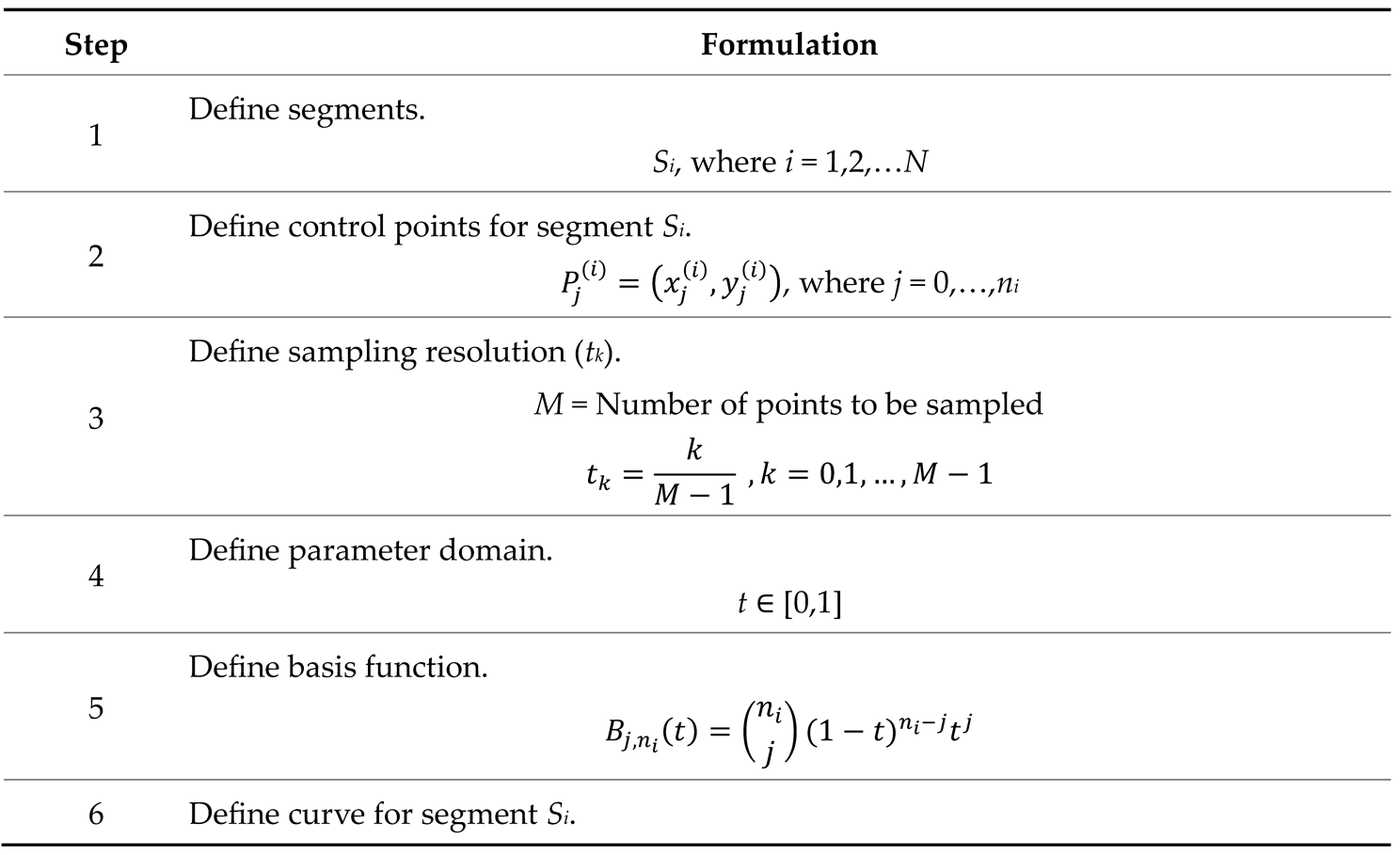 |
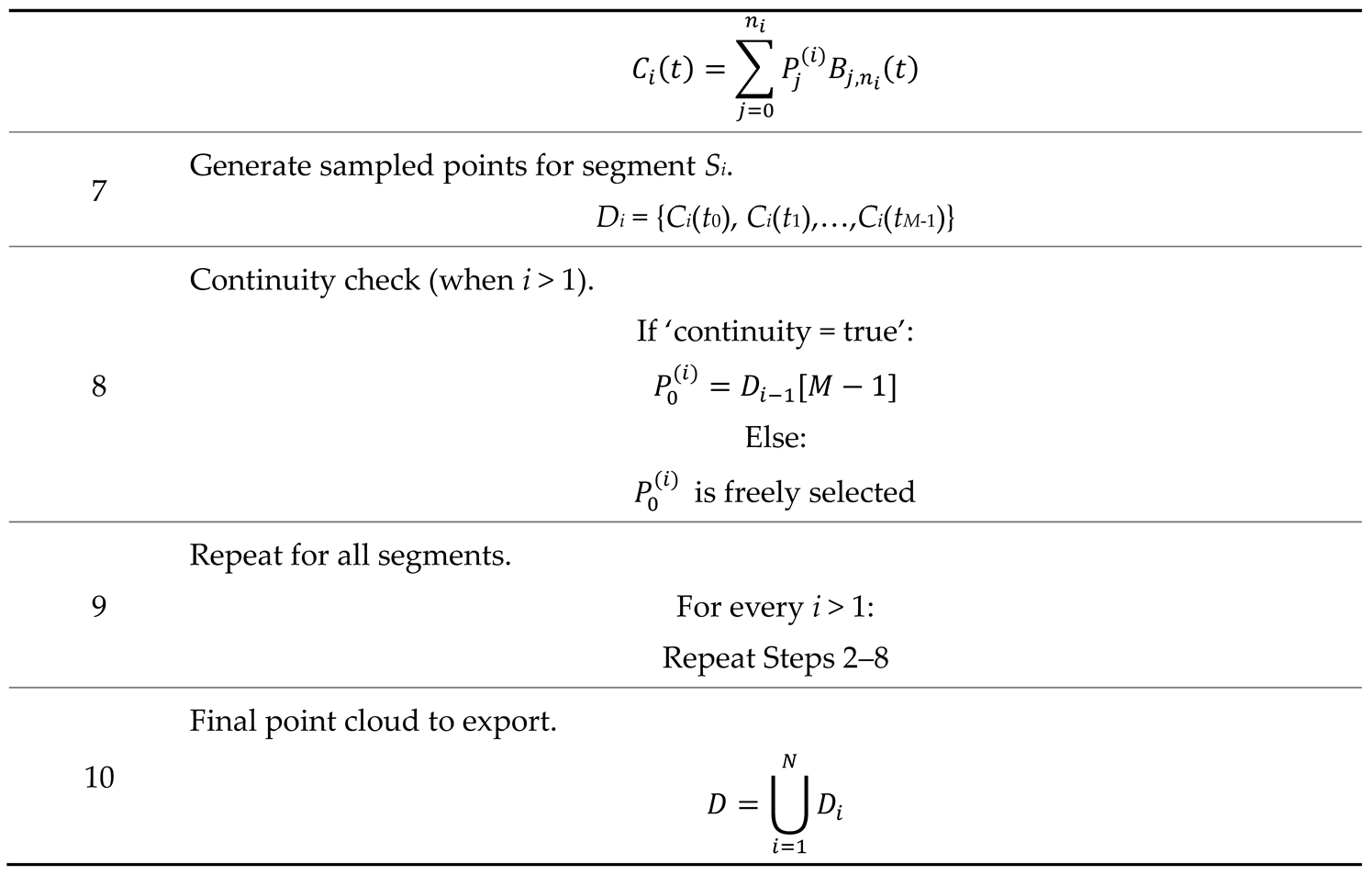 |
Table A3.
Formulations related to spline-based algorithm (System A2).
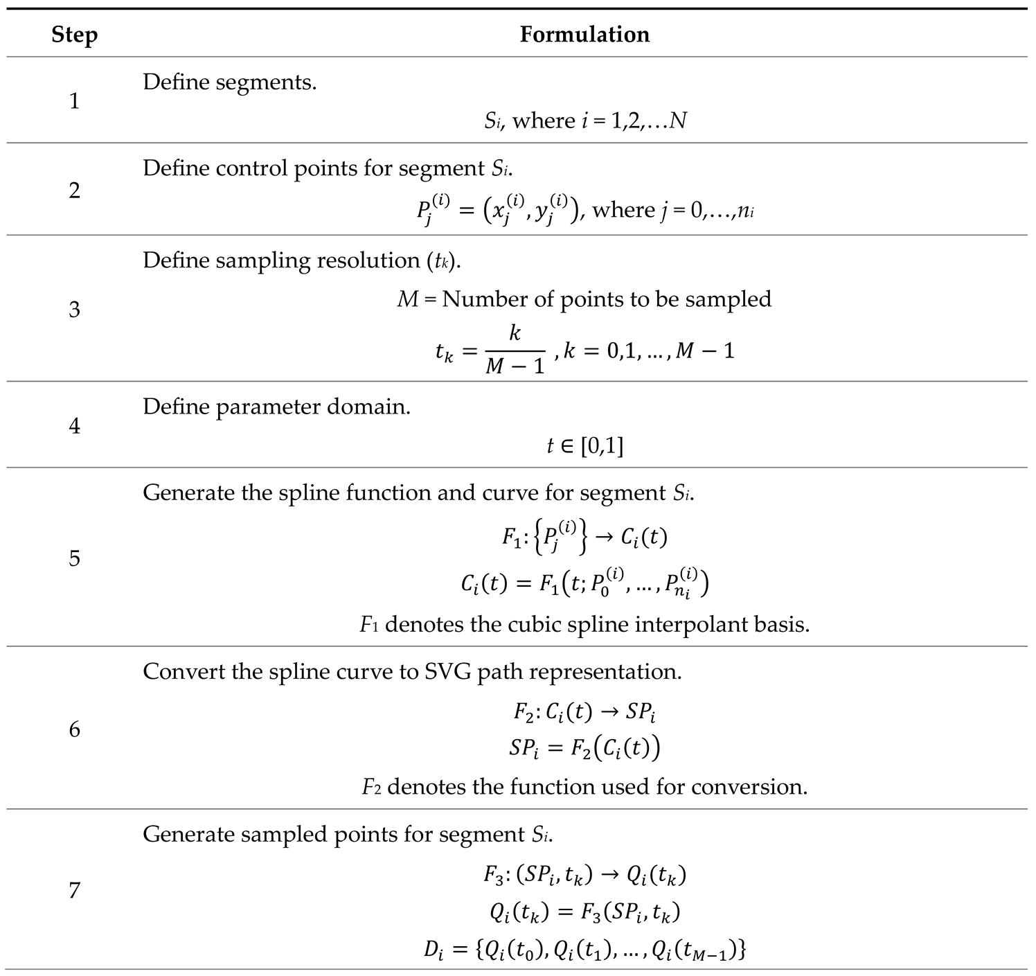 |
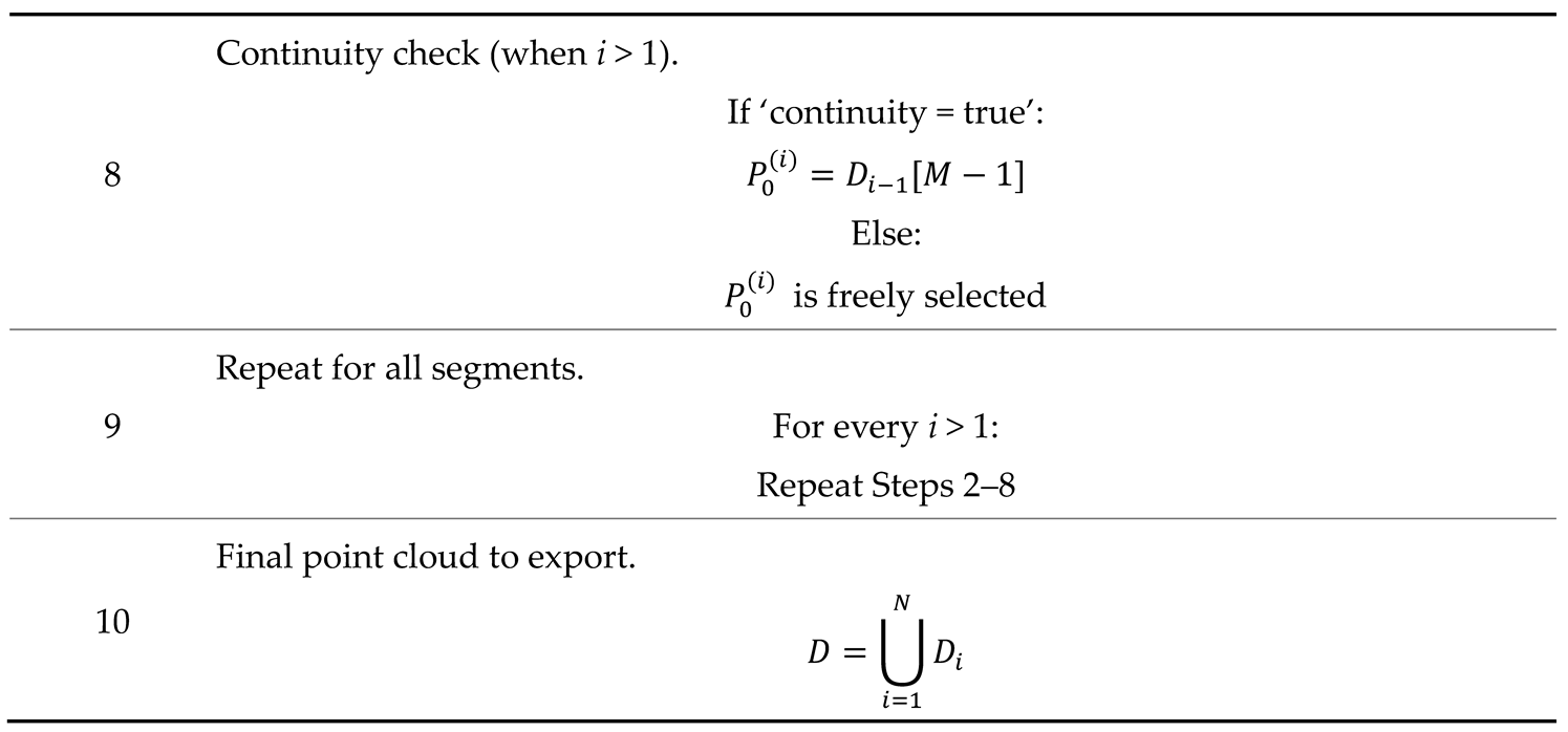 |
Appendix C. Formulations Related to System B (Section 4.1.2).
Table A4.
Formulations related to computing geometric shape’s point clouds.
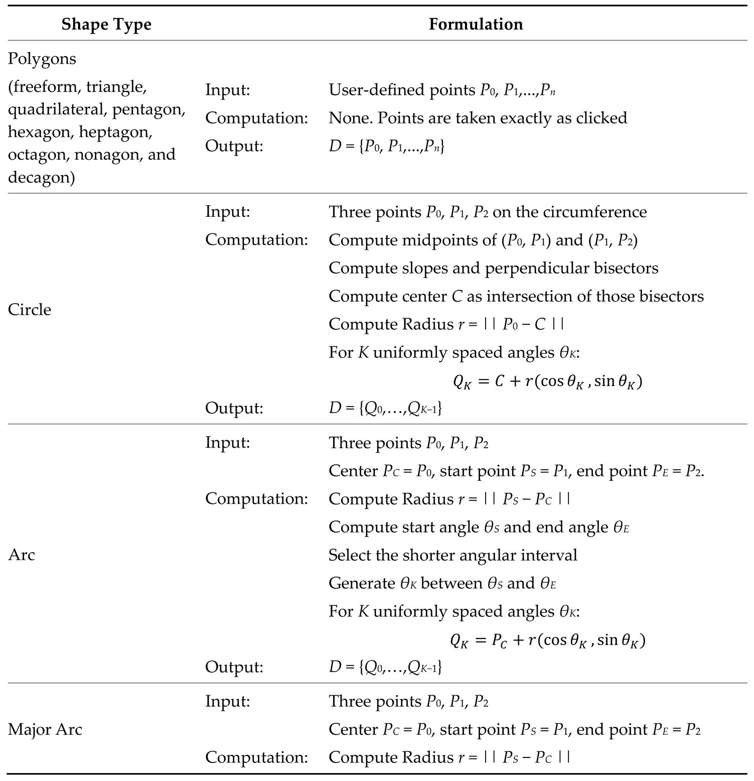 |
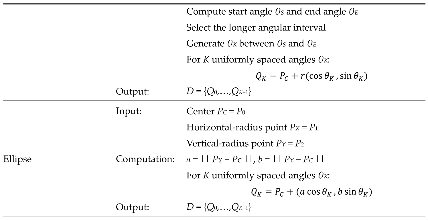 |
Appendix D. Formulations Related to System C (Section 4.1.3).
Table A5.
Formulations related to transforming a given set of points.
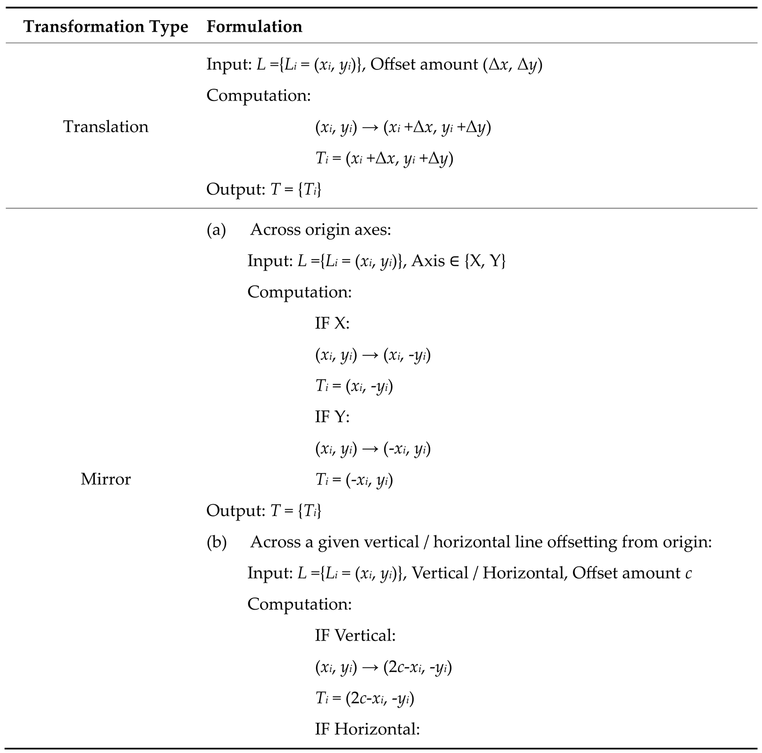 |
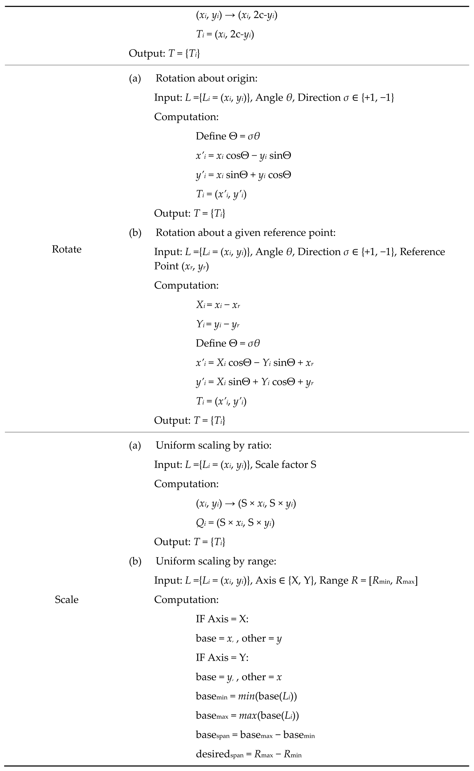 |
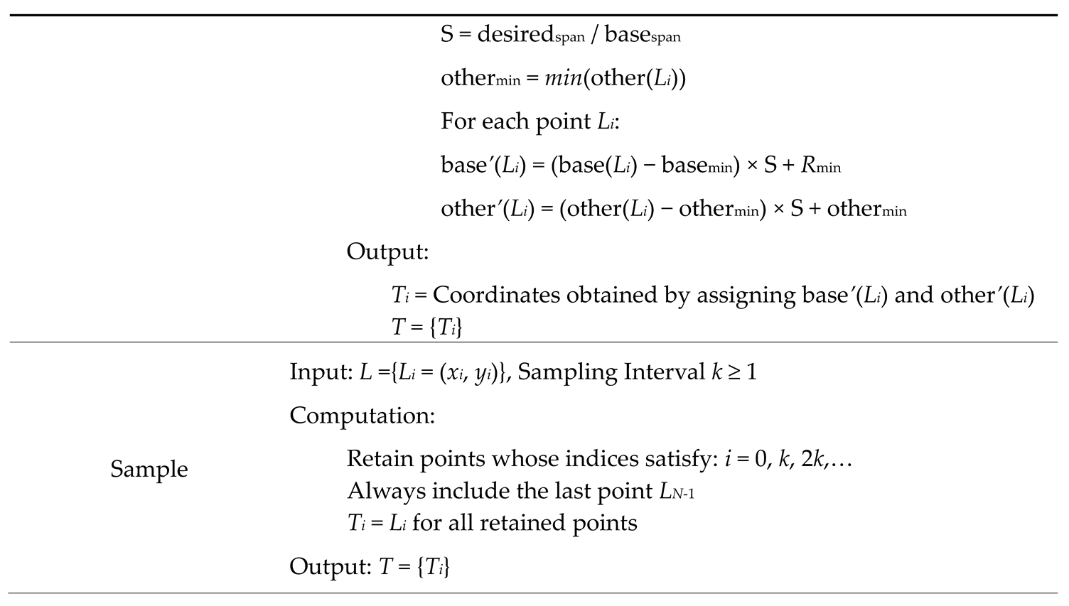 |
Appendix E. Formulations Related to System D (Section 4.1.4).
Table A6.
Formulations related to cleaning and sequencing a given set of points.
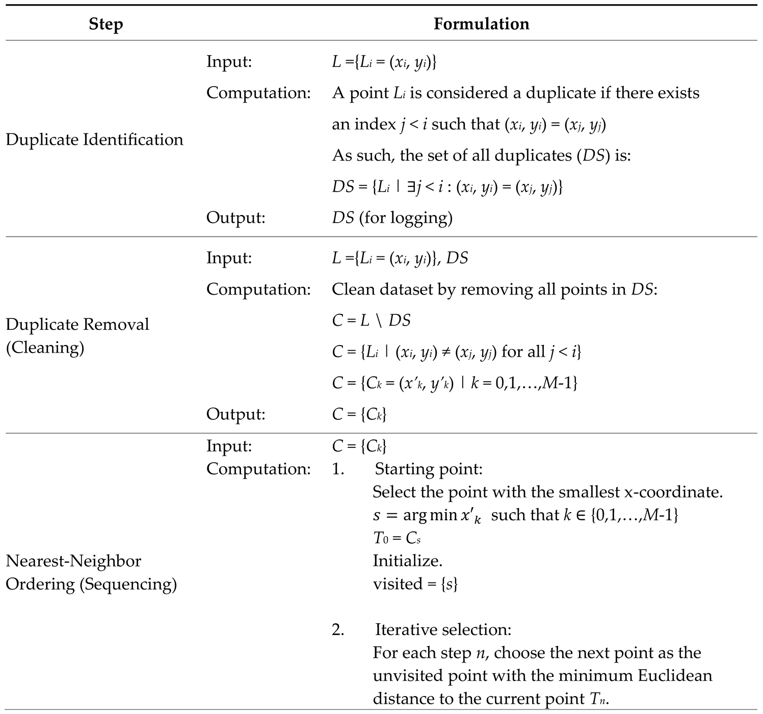 |
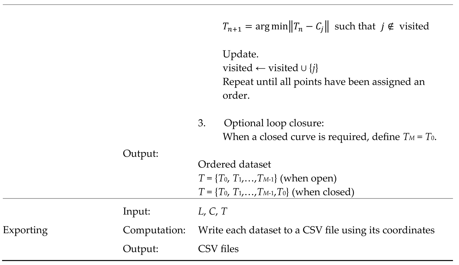 |
Appendix F. Developed Functions Related to OpenSCAD (Section 4.2).
Table A7.
Developed functions related to OpenSCAD.
| SN | Syntax | Input Arguments | Purpose (or Outcome) |
|---|---|---|---|
| 1 | close_path (points_set) | points_set: A list of 2D points [[x, y], [x, y],...] |
Returns a new point set with the first point appended to the end. |
| 2 | show_points (points_set, radius, fragments, col) | points_set: A list of 2D points. radius: Radius of the sphere at each point. fragments: Controls smoothness of the sphere (number of fragments). col: Color of the spheres (string name or RGB list). |
Displays each point as a sphere. |
| 3 | create_polygon (points_set) | points_set: A list of 2D points in the order of polygon vertices. |
Draws a filled 2D polygon using the provided point set. |
| 4 | extrude_polygon (points_set, height) | points_set: A list of 2D points in the order of polygon vertices. height: Extrusion height. |
Extrudes a 2D polygon. |
| 5 | create_2d_path (points_set, width, fragments, shape) | points_set: A list of 2D points. width: Diameter (for circle) or side length (for square). fragments: Controls smoothness (used only if shape is “circle”). shape: Shape type for drawing hull — “circle” or “square”. |
Creates a 2D path using hulls between either circles or squares. |
| 6 | extrude_2d_path (points_set, width, fragments, height, shape) | points_set: A list of 2D points. width: Diameter (for circle) or side length (for square). fragments: Controls smoothness (used only if shape is “circle”). height: Extrusion height. shape: Shape type for drawing hull — “circle” or “square”. |
Extrudes a 2D path based on either circles or squares. |
References
- Dym, C.L.; Agogino, A.M.; Eris, O.; Frey, D.D.; Leifer, L.J. Engineering Design Thinking, Teaching, and Learning. J. Eng. Educ. 2005, 94, 103–120. [Google Scholar] [CrossRef]
- MacMahon, C.; Browne, J. CADCAM: principles, practice and manufacturing management, 2. ed.; Prentice Hall: Harlow, England, 1998. [Google Scholar]
- Groover, M.P. Automation, production systems, and computer-integrated manufacturing, Fifth edition; Pearson: New York, 2018. [Google Scholar]
- Ullah, A.M.M.S.; Sato, M.; Watanabe, M.; Rashid, M. ; Bangladesh Institute of Management Integrating CAD, TRIZ, and Customer Needs. Int. J. Autom. Technol. 2016, 10, 132–143. [Google Scholar] [CrossRef]
- Black, I. Back to the future with CAD: its impact on product design and development. Des. Stud. 1990, 11, 207–211. [Google Scholar] [CrossRef]
- Kallis, D.; Fritz, W. CAD in engineering education: Getting the balance right. in 2009 3rd IEEE International Conference on E-Learning in Industrial Electronics (ICELIE), Porto: IEEE, Nov. 2009, pp. 36–39. [CrossRef]
- Brink, H.; Kilbrink, N.; Gericke, N. Teach to use CAD or through using CAD: An interview study with technology teachers. Int. J. Technol. Des. Educ. 2022, 33, 957–979. [Google Scholar] [CrossRef]
- Dougherty, D. The Maker Movement. Innov. Technol. Governance, Glob. 2012, 7, 11–14. [Google Scholar] [CrossRef]
- Pearce, J.M. Open-Source Lab; Elsevier: Amsterdam, Netherlands, 2014. [Google Scholar] [CrossRef]
- Armstrong, R. The Long Tail: Why the Future of Business Is Selling Less of More. Can. J. Commun. 2008, 33, 127–128. [Google Scholar] [CrossRef]
- Gershenfeld, N.A. Fab: the coming revolution on your desktop—from personal computers to personal fabrication, 1. ed.; Basic Books: New York, NY, 2005. [Google Scholar]
- Westerlund, M.; Leminen, S.; Rajahonka, M. Designing Business Models for the Internet of Things. Technol. Innov. Manag. Rev. 2014, 4, 5–14. [Google Scholar] [CrossRef]
- Koren, Y. The global manufacturing revolution: product-process-business integration and reconfigurable systems; Wiley: Hoboken, New Jersey, 2010. [Google Scholar]
- Kutari, L.D.; Ura, S. Analyzing Customer-Producer Interaction System Using Axiomatic Design Theory. Proc. Int. Conf. Des. Concurr. Eng. Manuf. Syst. Conf. 2023, 2023, 43. [Google Scholar] [CrossRef]
- Ghosh, A.K.; Rentzsch, M.; Ura, S. Fostering Empathy in AI-Driven Co-Creation of CAD Models. Procedia CIRP 2025, 134, 741–746. [Google Scholar] [CrossRef]
- Rayna, T.; Striukova, L. The Impact of 3D Printing Technologies on Business Model Innovation. in Digital Enterprise Design & Management, vol. 261, P. Benghozi, D. Krob, A. Lonjon, and H. Panetto, Eds., in Advances in Intelligent Systems and Computing, vol. 261. , Cham: Springer International Publishing, 2014, pp. 119–132. [CrossRef]
- Tadokoro, F.; Ghosh, A.K.; Ura, S. On the effective co-creation of CAD models by leveraging generative artificial intelligence. Procedia CIRP 2025, 134, 663–668. [Google Scholar] [CrossRef]
- OpenSCAD — The Programmers’ Solid 3D CAD Modeller. [Online]. Available: https://openscad.org/.
- CadQuery contributors, CadQuery. (Oct. 28, 2025). Zenodo. [CrossRef]
- Kopowski, J.; Mreła, A.; Mikołajewski, D.; Rojek, I. Enhancing 3D Printing with Procedural Generation and STL Formatting Using Python. Appl. Sci. 2024, 14, 7299. [Google Scholar] [CrossRef]
- Xie, H.; Ju, F. Text-to-CadQuery: A New Paradigm for CAD Generation with Scalable Large Model Capabilities. arXiv 2025. [Google Scholar] [CrossRef]
- Gómez-De-Gabriel, J.M.; Muñoz-Ramírez, A.J.; Palacios, M.; Parras, L. Rapid end-of-arm-tooling manufacturing of vacuum grippers. Int. J. Comput. Integr. Manuf. 2019, 32, 1231–1241. [Google Scholar] [CrossRef]
- Deng, H.; Khan, S.; Erkoyuncu, J.A. An Investigation on Utilizing Large Language Model for Industrial Computer-Aided Design Automation. Procedia CIRP 2024, 128, 221–226. [Google Scholar] [CrossRef]
- Machado, F.; Malpica, N.; Borromeo, S. Parametric CAD modeling for open source scientific hardware: Comparing OpenSCAD and FreeCAD Python scripts. PLOS ONE 2019, 14, e0225795. [Google Scholar] [CrossRef] [PubMed]
- Gonzalez, J.F.; Pietrzak, T.; Girouard, A.; Casiez, G. Facilitating the Parametric Definition of Geometric Properties in Programming-Based CAD. In Proceedings of the 37th Annual ACM Symposium on User Interface Software and Technology, Oct. 2024, Pittsburgh PA USA: ACM; pp. 1–12. [CrossRef]
- Makatura, L.; et al. How Can Large Language Models Help Humans in Design and Manufacturing? arXiv 2023. [Google Scholar] [CrossRef]
- Makatura, L.; Foshey, M.; Wang, B.; Hähnlein, F.; Ma, P.; Deng, B.; Tjandrasuwita, M.; Spielberg, A.; Owens, C.; Chen, P.Y.; et al. How Can Large Language Models Help Humans in Design and Manufacturing? Part 1: Elements of the LLM-Enabled Computational Design and Manufacturing Pipeline. Harvard Data Science Review 2023. [Google Scholar] [CrossRef]
- Makatura, L.; Foshey, M.; Wang, B.; Hähnlein, F.; Ma, P.; Deng, B.; Tjandrasuwita, M.; Spielberg, A.; Owens, C.; Chen, P.Y.; et al. How Can Large Language Models Help Humans in Design And Manufacturing? Part 2: Synthesizing an End-to-End LLM-Enabled Design and Manufacturing Workflow. Harvard Data Science Review 2023. [Google Scholar] [CrossRef]
- Filz, M.-A.; Thiede, S. Generative AI in Manufacturing Systems: Reference Framework and Use Cases. Procedia CIRP 2024, 130, 238–243. [Google Scholar] [CrossRef]
- Nelson, M.D.; Goenner, B.L.; Gale, B.K. Utilizing ChatGPT to assist CAD design for microfluidic devices. Lab a Chip 2023, 23, 3778–3784. [Google Scholar] [CrossRef]
- Avila, J.F.G.; Pietrzak, T.; Girouard, A.; Casiez, G. Understanding the Challenges of OpenSCAD Users for 3D Printing. In Proceedings of the CHI Conference on Human Factors in Computing Systems, Honolulu HI USA, May 2024; pp. 1–20. [Google Scholar] [CrossRef]
- Mahapatra, C.; Jensen, J.K.; McQuaid, M.; Ashbrook, D. Barriers to End-User Designers of Augmented Fabrication. In Proceedings of the 2019 CHI Conference on Human Factors in Computing Systems, Glasgow Scotland Uk: ACM, May 2019; pp. 1–15. [Google Scholar] [CrossRef]
- The Double Diamond—Design Council.” Accessed: Nov. 23, 2025. [Online]. Available: https://www.designcouncil.org.uk/our-resources/the-double-diamond/.
- Hatchuel, A.; Weil, B. C-K design theory: an advanced formulation. Res. Eng. Des. 2008, 19, 181–192. [Google Scholar] [CrossRef]
- Kutari, L.D.; Ura, S. Improving reverse engineering processes using C-K theory of design. Res. Eng. Des. 2025, 36, 1–17. [Google Scholar] [CrossRef]
- Tashi; Ullah, A.S.; Watanabe, M.; Kubo, A. Analytical Point-Cloud Based Geometric Modeling for Additive Manufacturing and Its Application to Cultural Heritage Preservation. Appl. Sci. 2018, 8, 656. [CrossRef]
- Tashi; Ullah, A.M.M.S.; Kubo, A.; Tashi, T. Developing a Human-Cognition-Based Reverse Engineering Approach. In Proceedings of the JSME 2020 Conference on Leading Edge Manufacturing/Materials and Processing, Virtual, Online, Sept. 2020. [CrossRef]
- Farin, G. The Bernstein Form of a Bézier Curve. In Curves and Surfaces for CAGD, Elsevier, 2002; pp. 57–79. [CrossRef]
- Computer graphics: principles and practice, 2. ed.; in C, Reprinted with corr., 25. print. in The systems programming series; Foley, J.D., Ed.; Addison-Wesley: Bosto, 2010. [Google Scholar]
- Bostock, M.; Ogievetsky, V.; Heer, J. D³ Data-Driven Documents. IEEE Trans. Vis. Comput. Graph. 2011, 17, 2301–2309. [Google Scholar] [CrossRef] [PubMed]
- What is D3?” Accessed: Nov. 23, 2025. [Online]. Available: https://d3js.org/what-is-d3.
- D3.js: Data-Driven Documents. Accessed: Nov. 23, 2025. [Online]. Available: https://d3js.org/.
- Plotly.js: Open-Source JavaScript Graphing Library. Accessed: Nov. 23, 2025. [Online]. Available: https://plotly.com/javascript/.
- Welcome to Python.org. Available online: https://www.python.org/ (accessed on 3 April 2022).
- McKinney, W. Data structures for statistical computing in python. In Proceedings of the 9th Python in Science Conference, Austin, TX, USA, 28 June–3 July 2010; Volume 445, pp. 51–56. [Google Scholar]
- Virtanen, P.; Gommers, R.; Oliphant, T.E.; Haberland, M.; Reddy, T.; Cournapeau, D.; Burovski, E.; Peterson, P.; Weckesser, W.; Bright, J.; et al. SciPy 1.0: Fundamental Algorithms for Scientific Computing in Python. Nat. Methods 2020, 17, 261–272. [Google Scholar] [CrossRef] [PubMed]
- Hunter, J.D. Matplotlib: A 2D graphics environment. Comput. Sci. Eng. 2007, 9, 90–95. [Google Scholar] [CrossRef]
- jExcel: Lightweight JavaScript Data Grid (Community Edition, MIT License). Accessed: Nov. 23, 2025. [Online]. Available: https://github.com/jspreadsheet/ce.
- jSuites UI Library. jSuites — JavaScript UI Components. Accessed: Nov. 23, 2025. [Online]. Available: https://jsuites.net/.
Figure 1.
Basic CAD workflow in (a) traditional and (b) script-based environments.
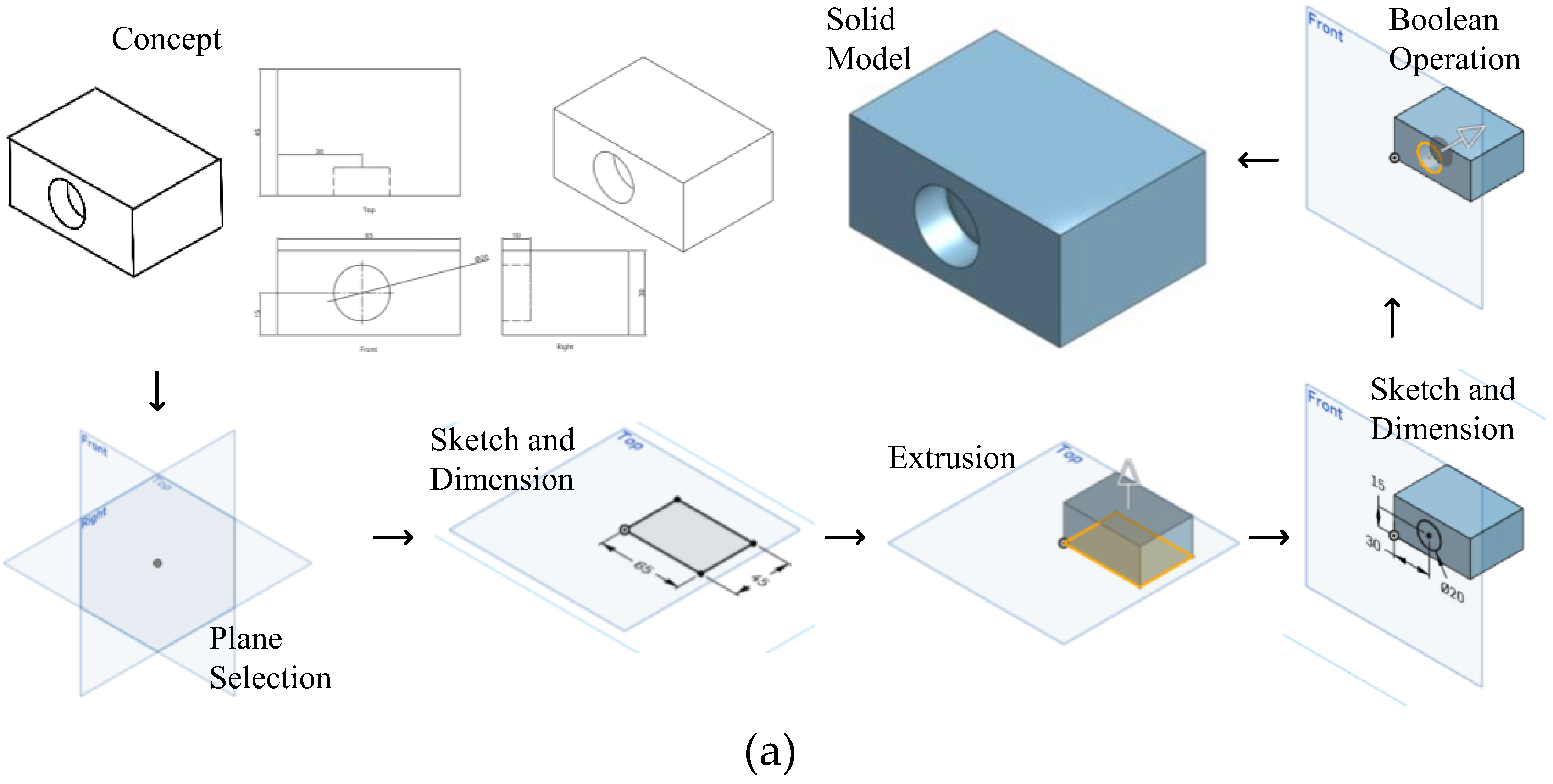
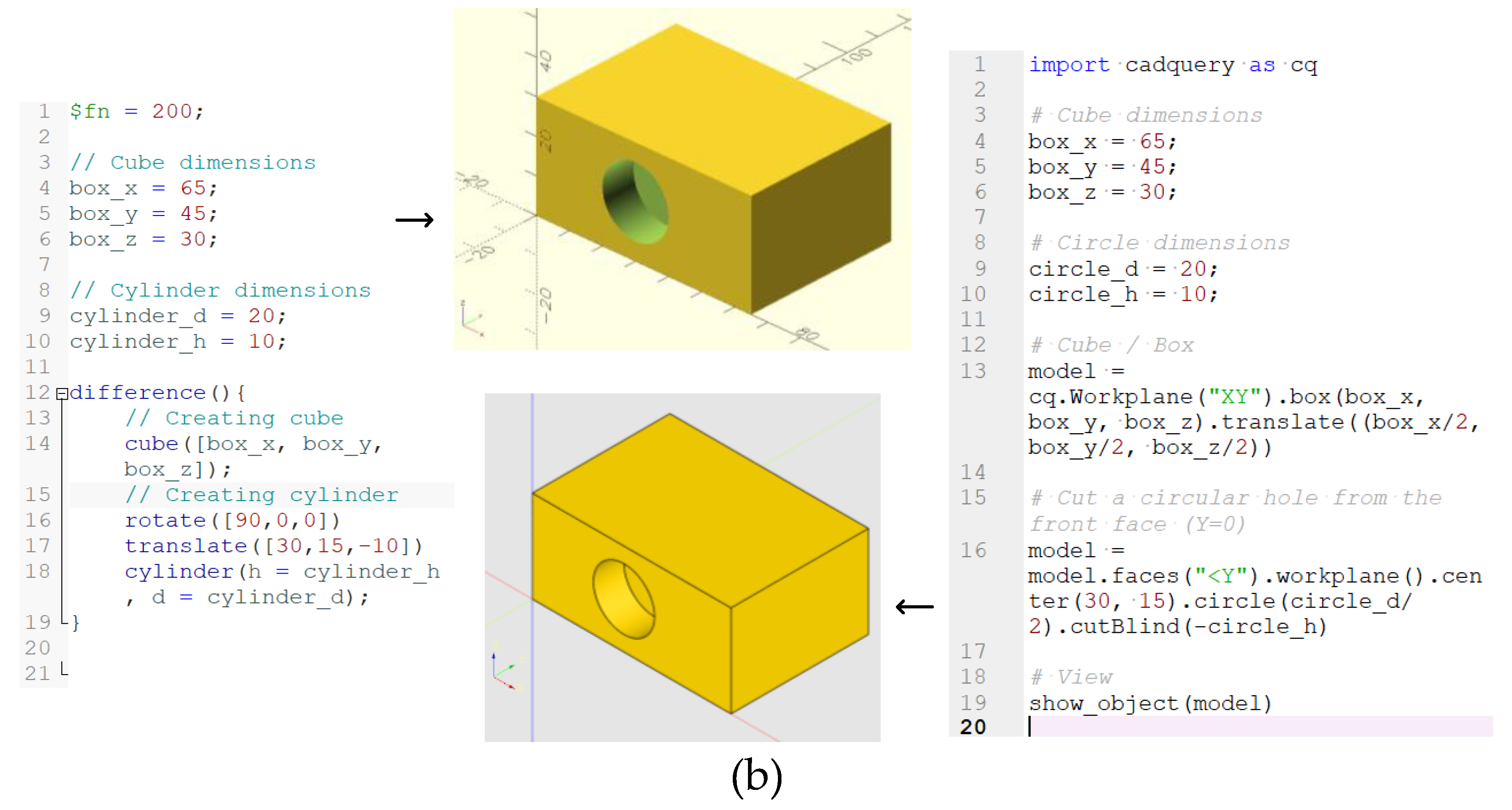
Figure 2.
Example free-form and irregular shapes.
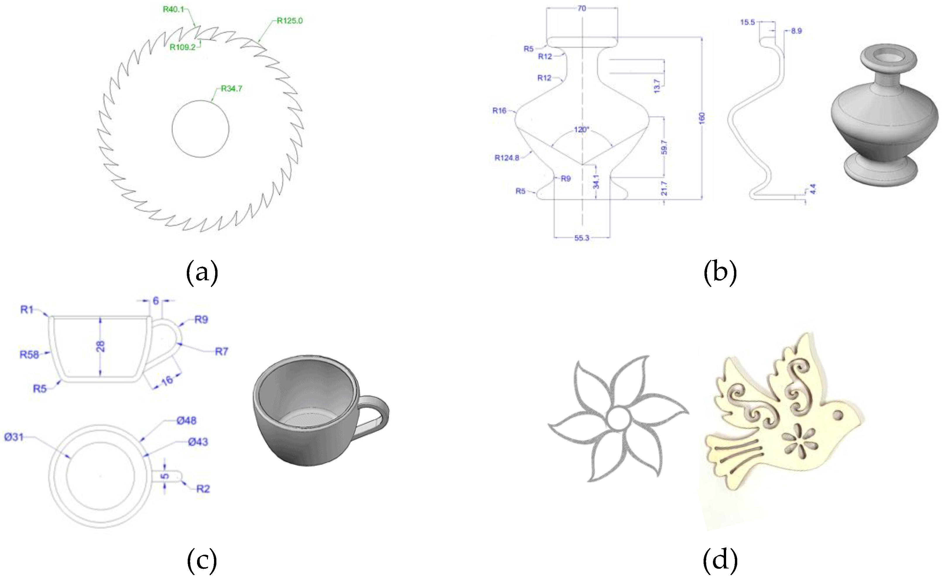
Figure 3.
Example shape.
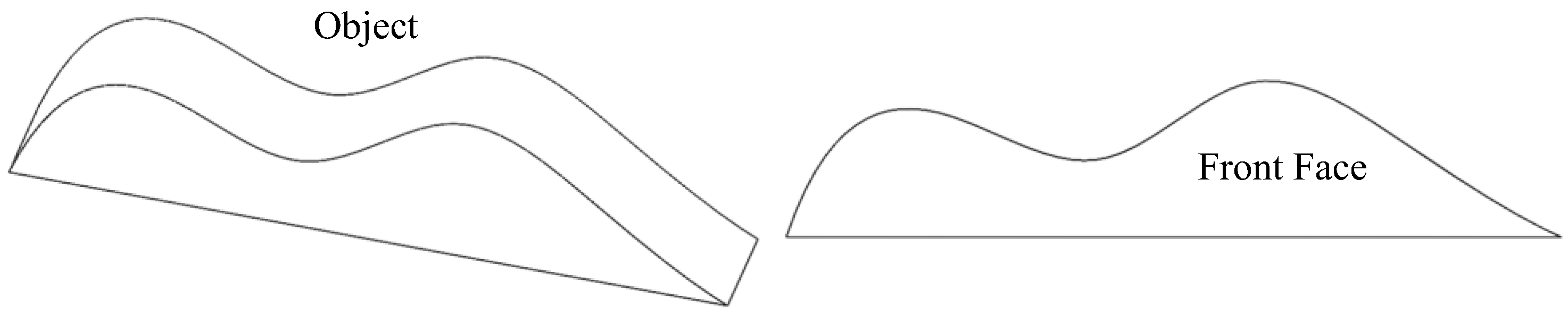
Figure 4.
Example CQ code and outcome for modeling the shape in Figure 3.
Figure 4.
Example CQ code and outcome for modeling the shape in Figure 3.
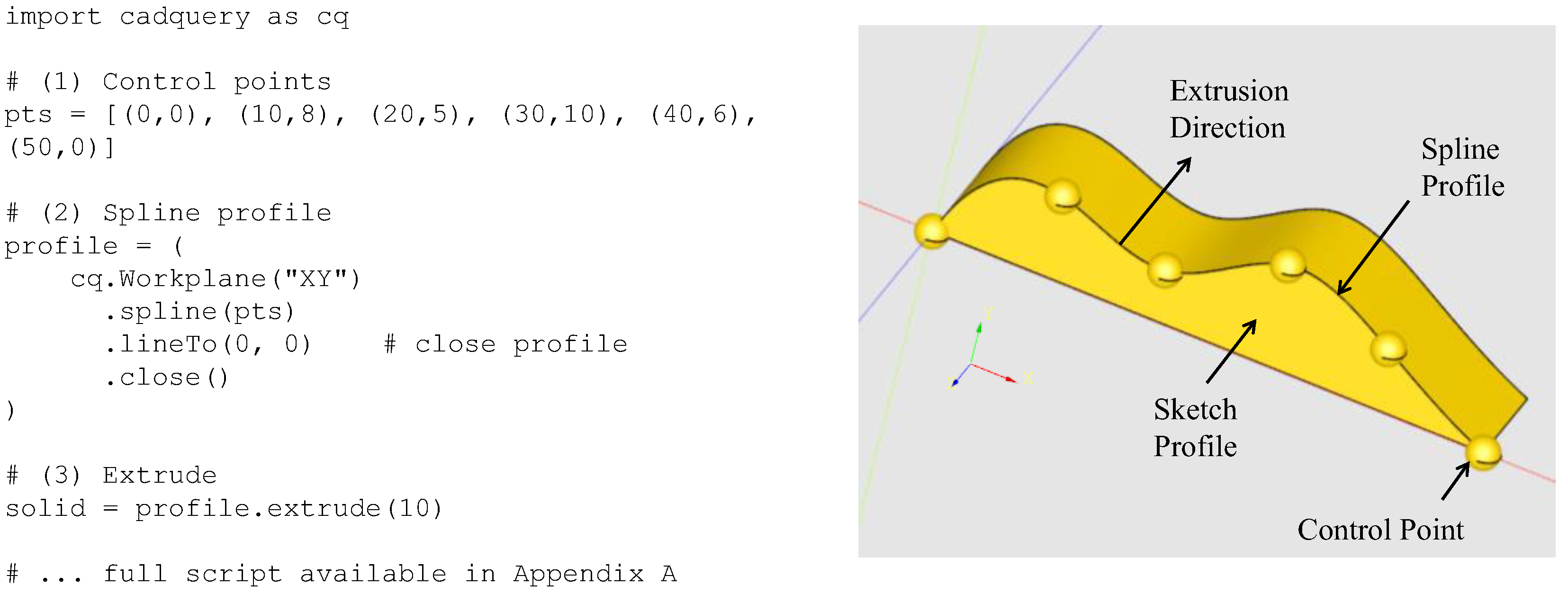
Figure 5.
Example OpenSCAD code and outcome for modeling the shape in Figure 3.
Figure 5.
Example OpenSCAD code and outcome for modeling the shape in Figure 3.
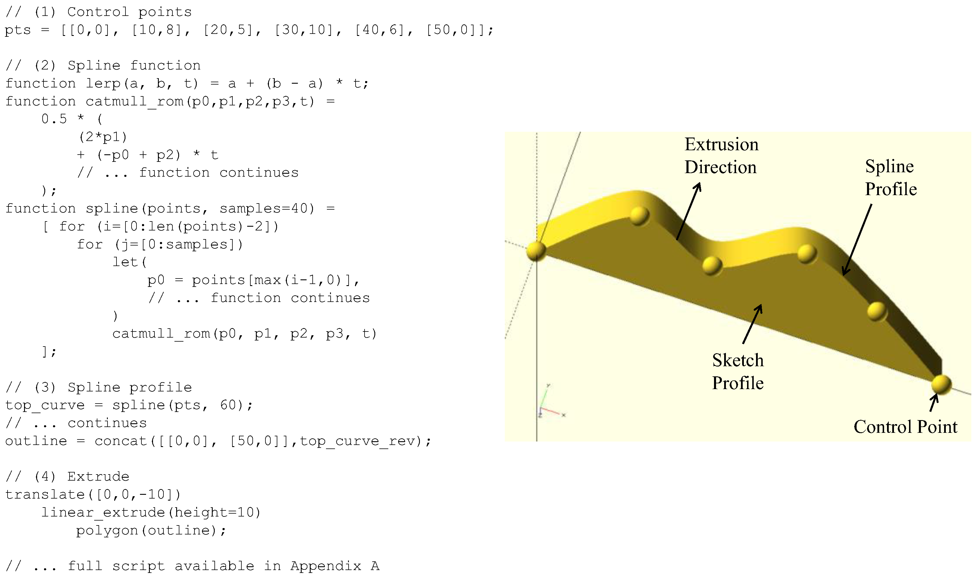
Figure 6.
Proposed CAD framework.
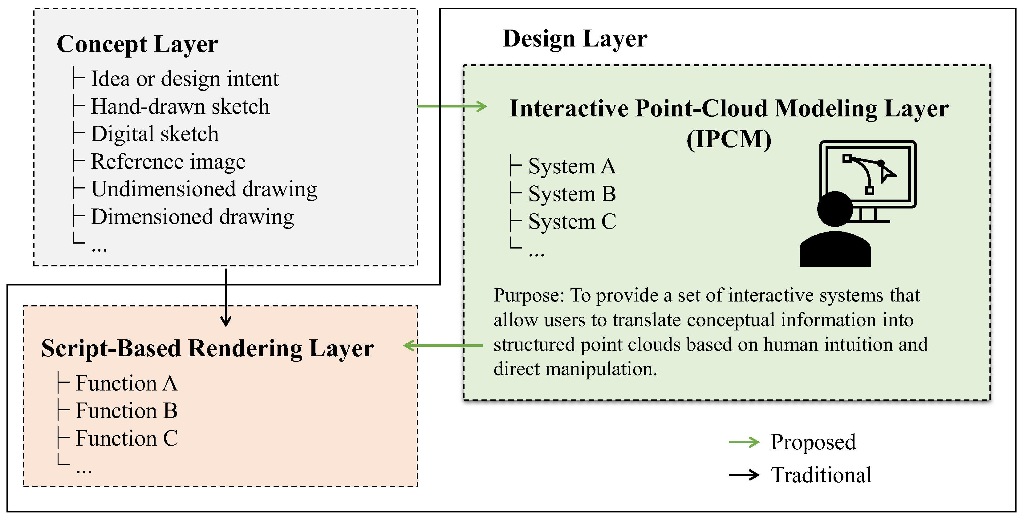
Figure 7.
Outlining the use of proposed framework.
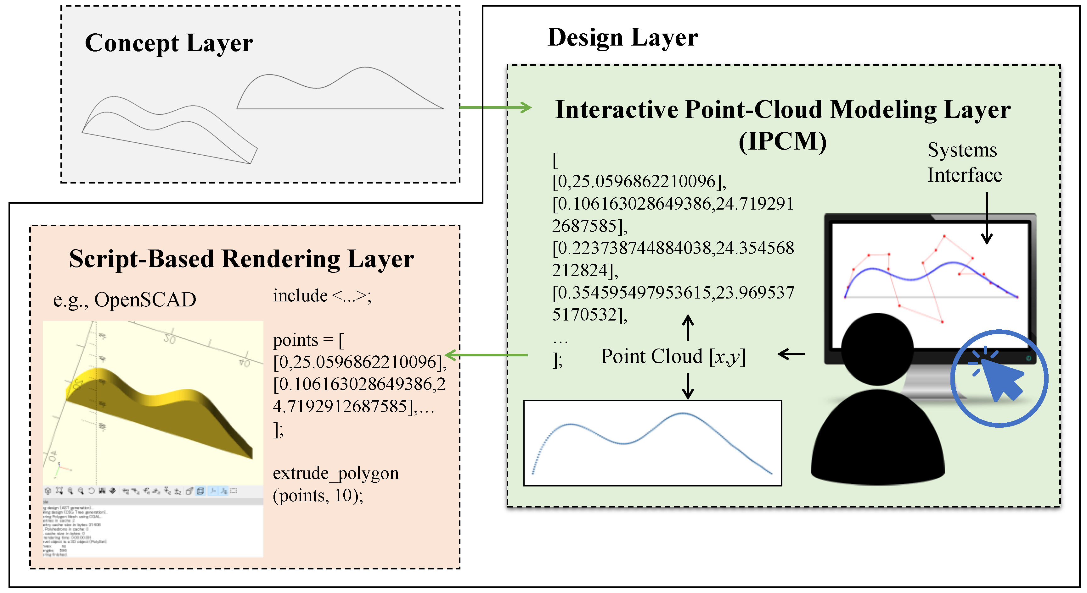
Figure 8.
Outline of the System A workflow.
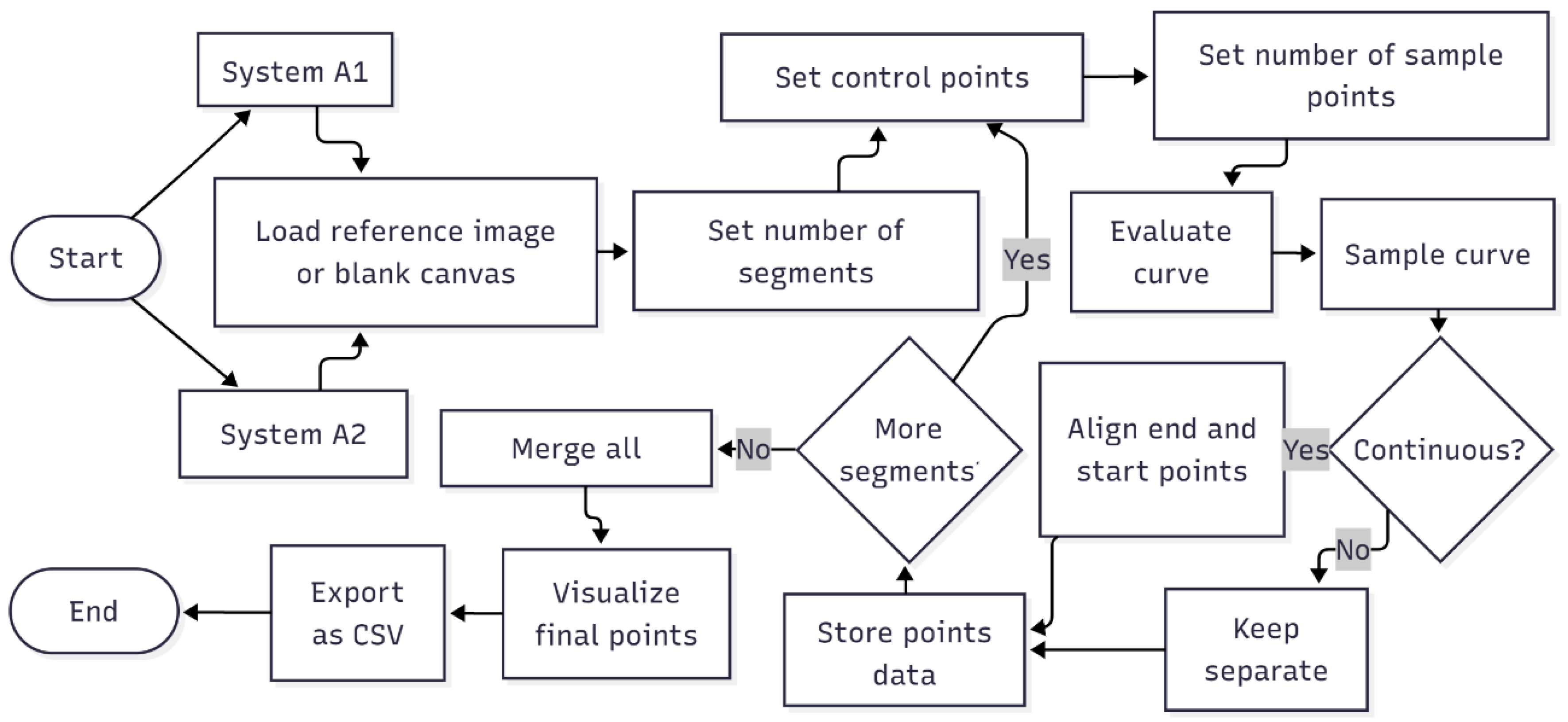
Figure 9.
Outline of the System B workflow.
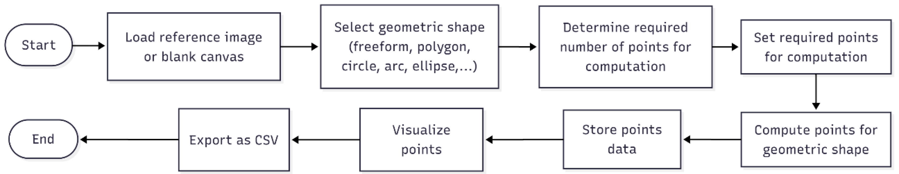
Figure 10.
Outline of the System C workflow.
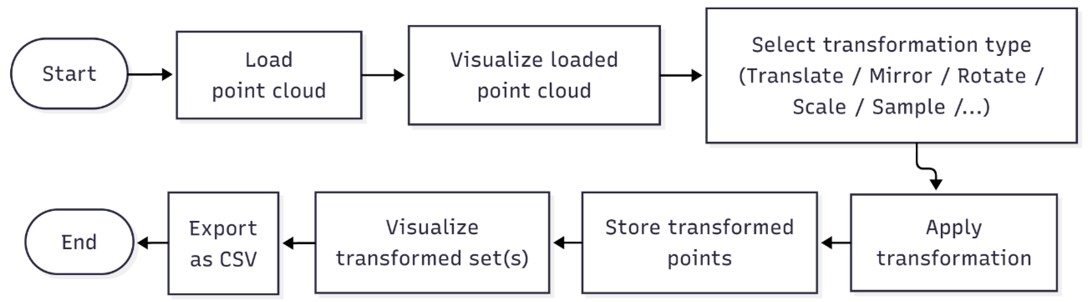
Figure 11.
Outline of the System D workflow.
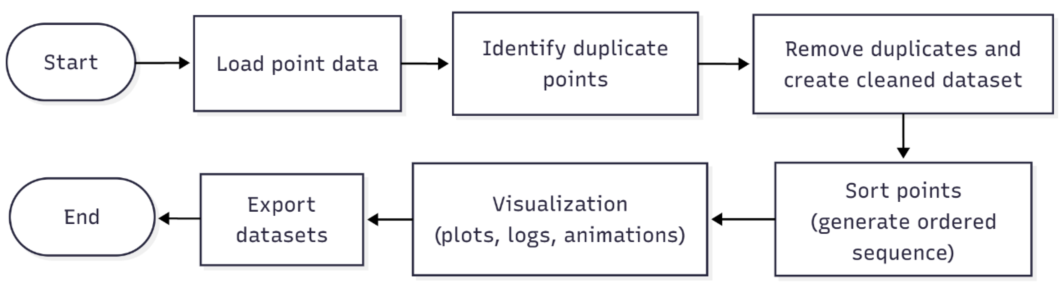
Figure 12.
Outline of the System E workflow.
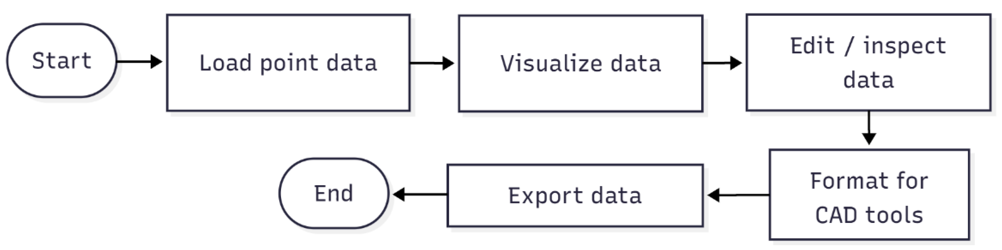
Figure 13.
Screenprint of the online portal for IPCM Layer.

Figure 14.
Generating points in the IPCM layer for the concept in Figure 2(a).
Figure 14.
Generating points in the IPCM layer for the concept in Figure 2(a).

Figure 15.
Rendering and constructing CAD model from the generated points in Figure 14.
Figure 15.
Rendering and constructing CAD model from the generated points in Figure 14.
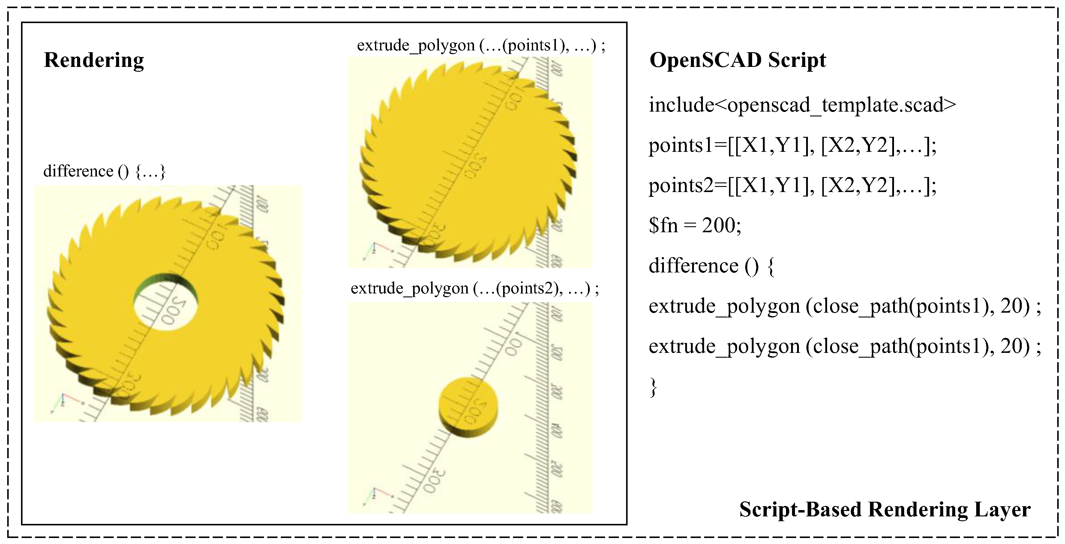
Figure 16.
Generating points in the IPCM layer for the concept in Figure 2(b).
Figure 16.
Generating points in the IPCM layer for the concept in Figure 2(b).
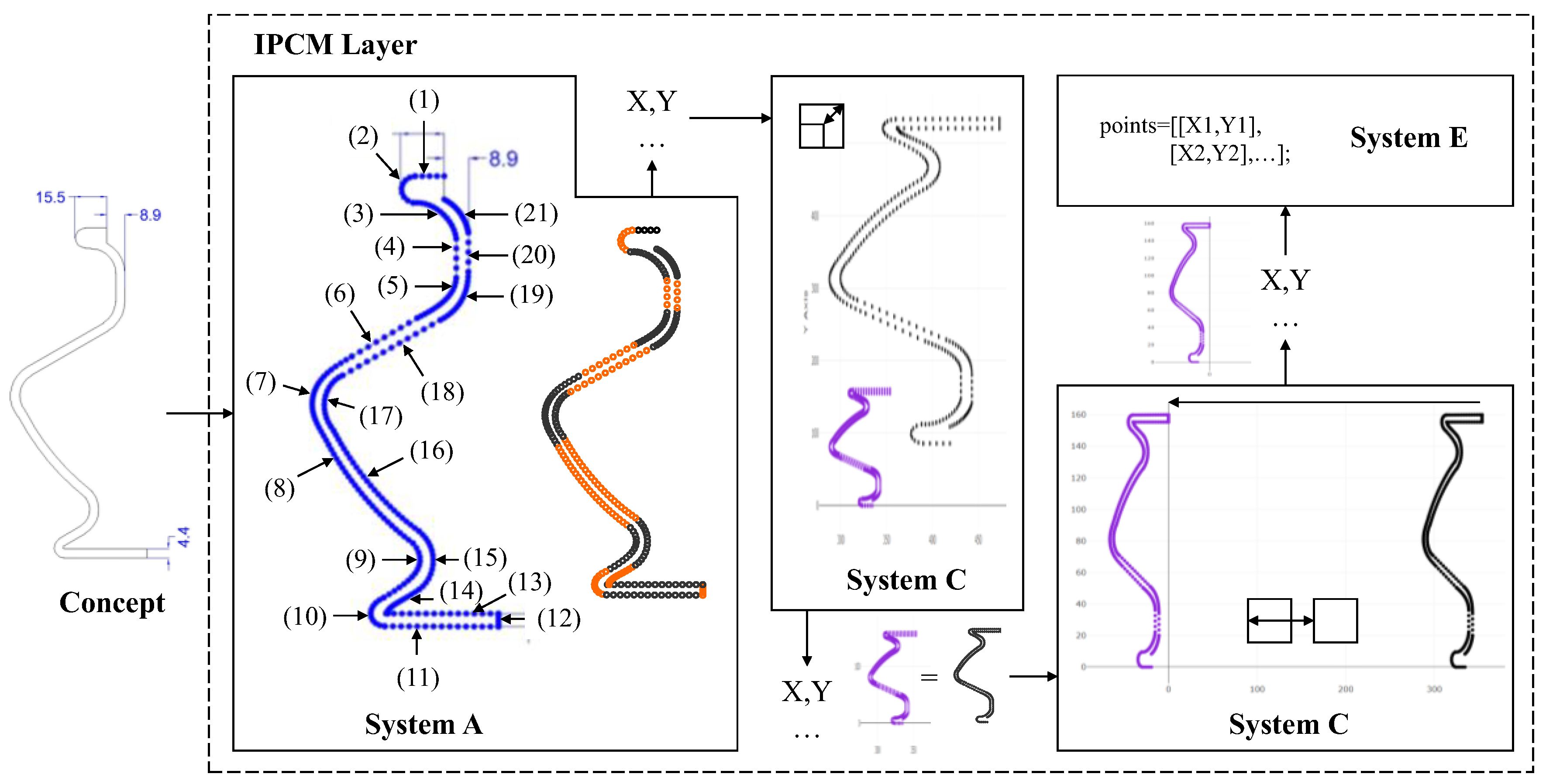
Figure 17.
Rendering and constructing CAD model from the generated points in Figure 16.
Figure 17.
Rendering and constructing CAD model from the generated points in Figure 16.
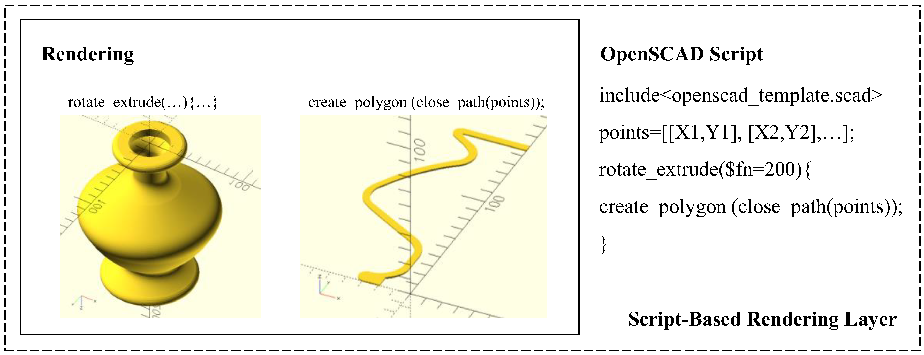
Figure 18.
Generating points in the IPCM layer for the concept in Figure 2(c).
Figure 18.
Generating points in the IPCM layer for the concept in Figure 2(c).
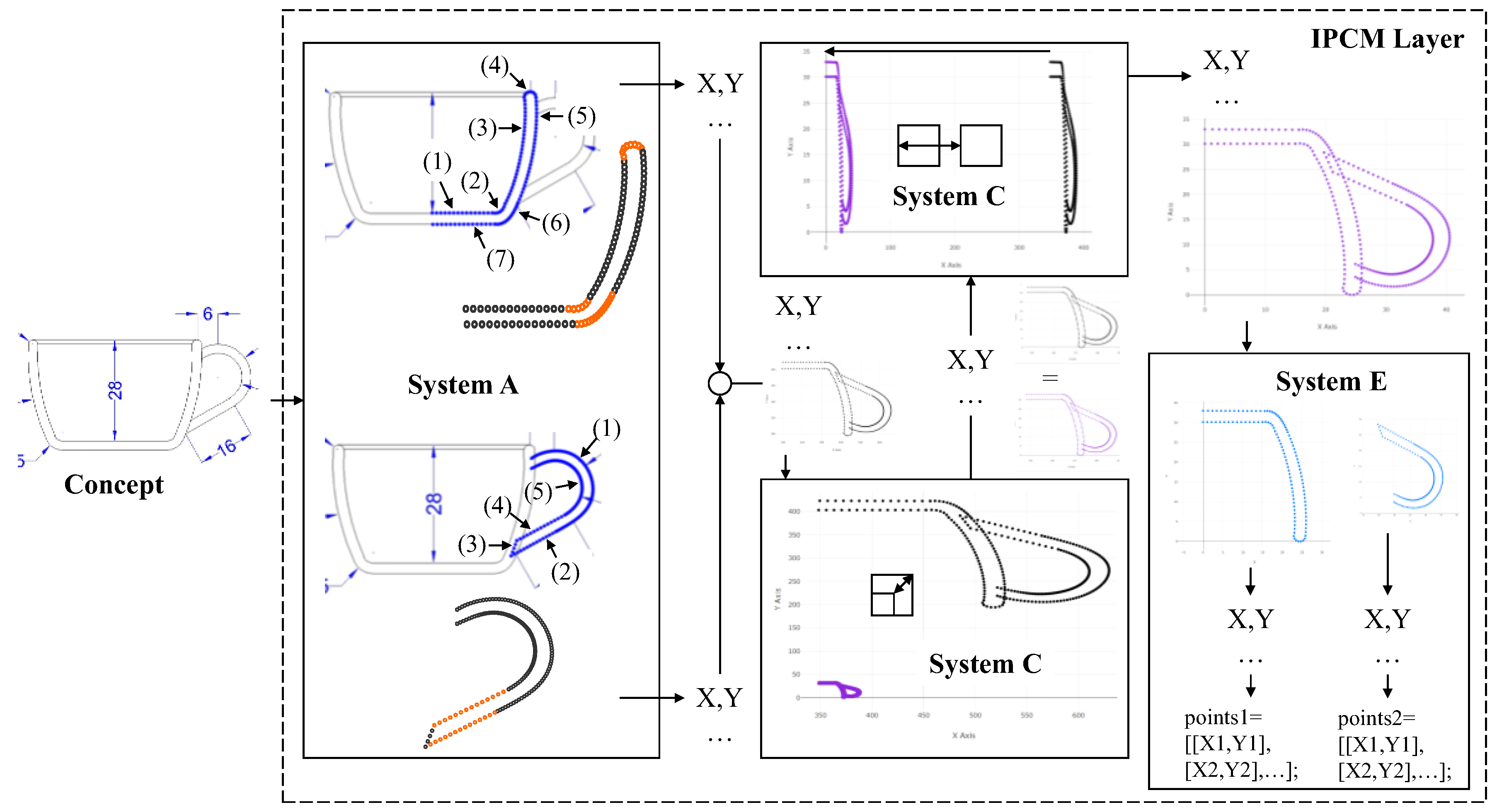
Figure 19.
Rendering and constructing CAD model from the generated points in Figure 18.
Figure 19.
Rendering and constructing CAD model from the generated points in Figure 18.
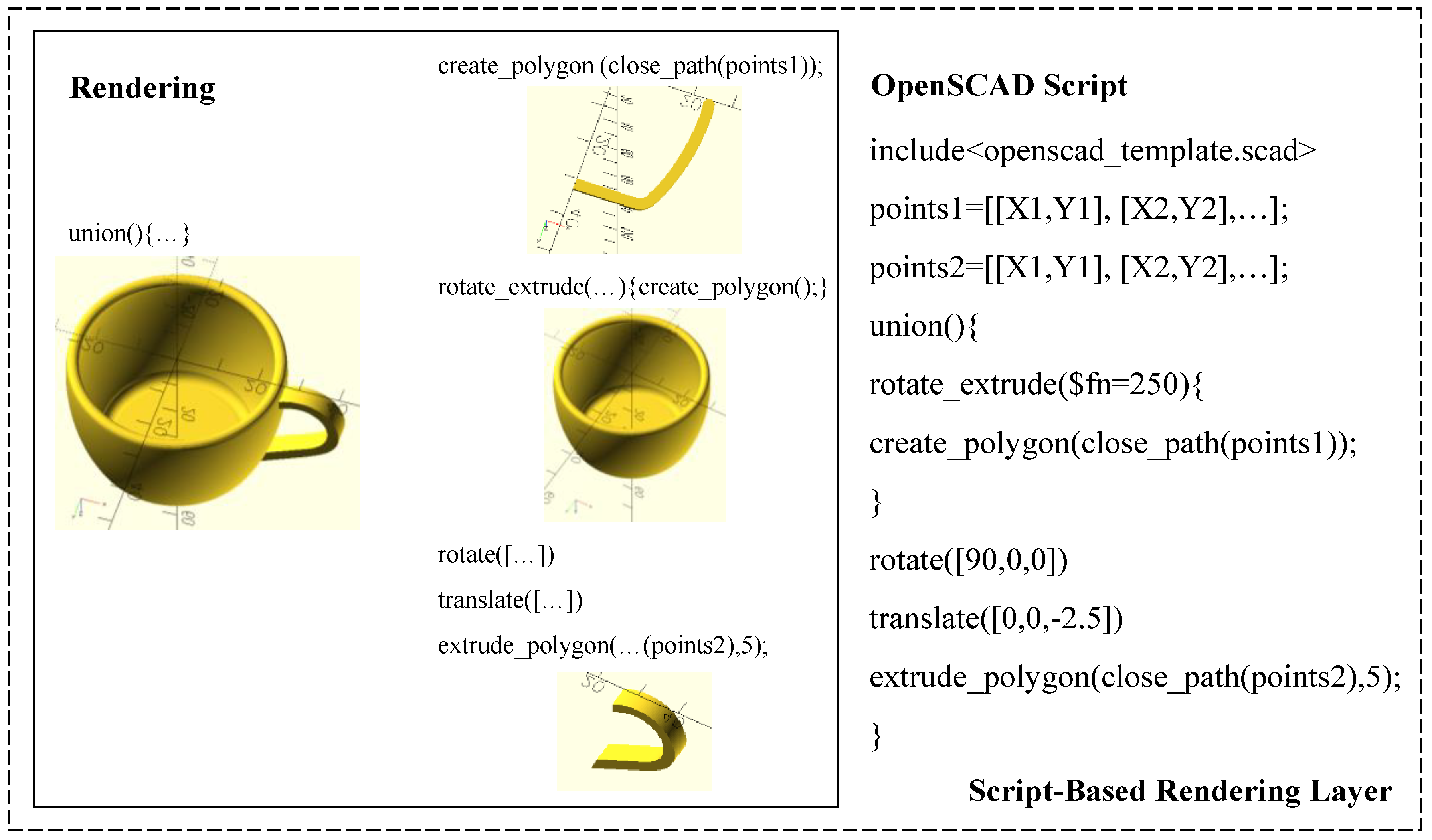
Figure 20.
Generating points in the IPCM layer for the concept in Figure 2(d).
Figure 20.
Generating points in the IPCM layer for the concept in Figure 2(d).
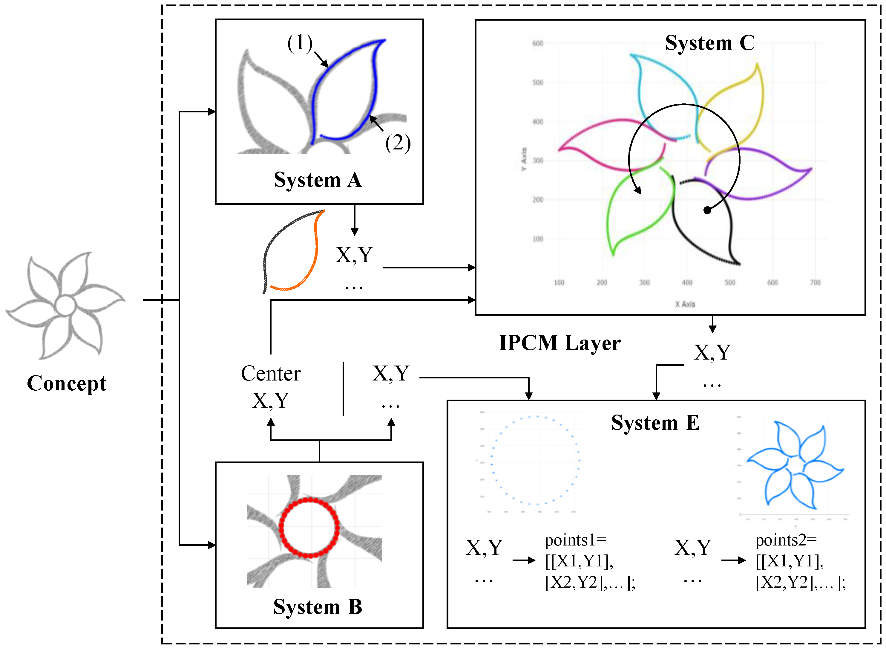
Figure 21.
Rendering and constructing CAD model from the generated points in Figure 20.
Figure 21.
Rendering and constructing CAD model from the generated points in Figure 20.
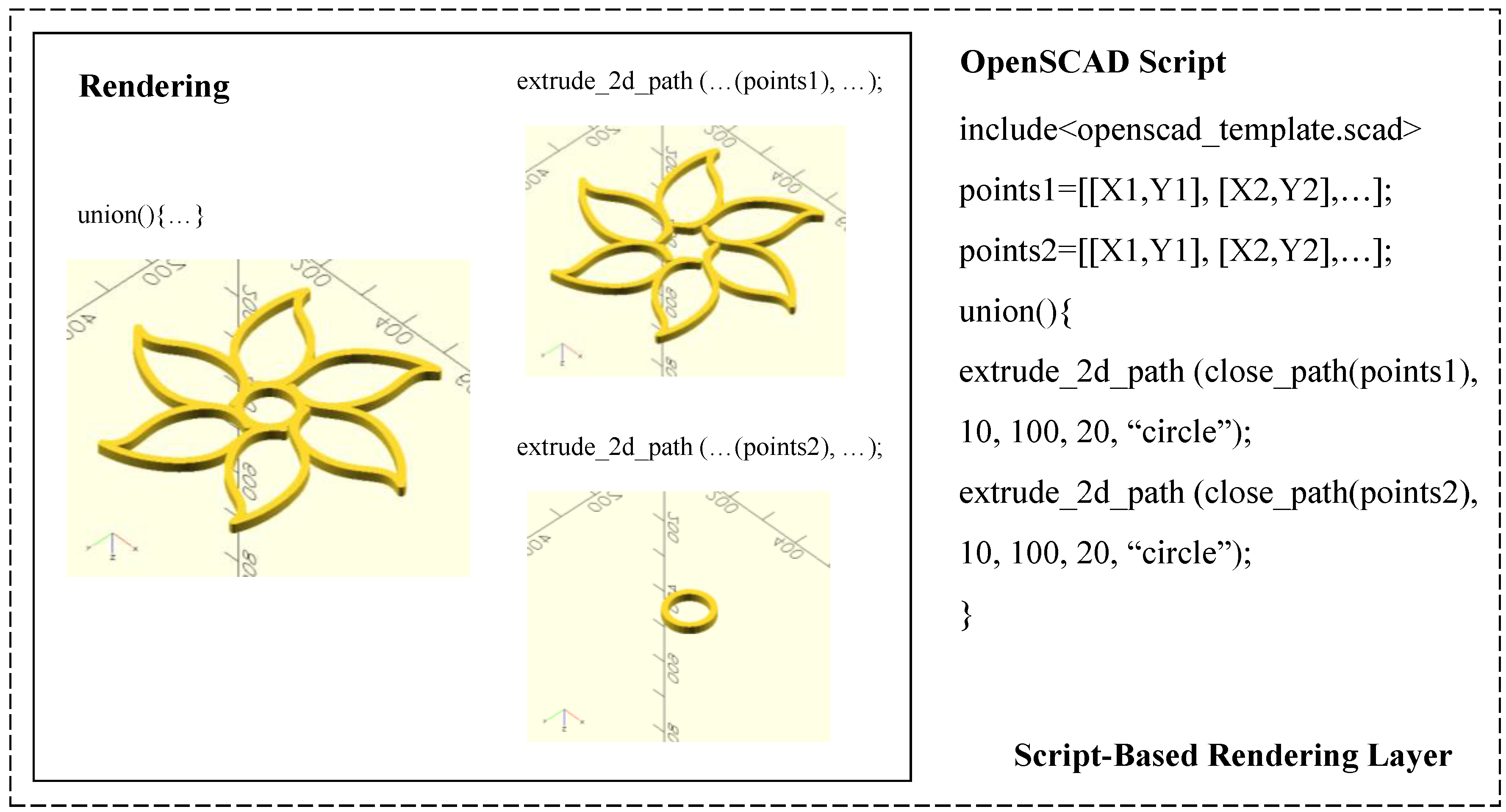
Figure 22.
Generating points in the IPCM layer for the concept in Figure 2(d) (bird motif).
Figure 22.
Generating points in the IPCM layer for the concept in Figure 2(d) (bird motif).
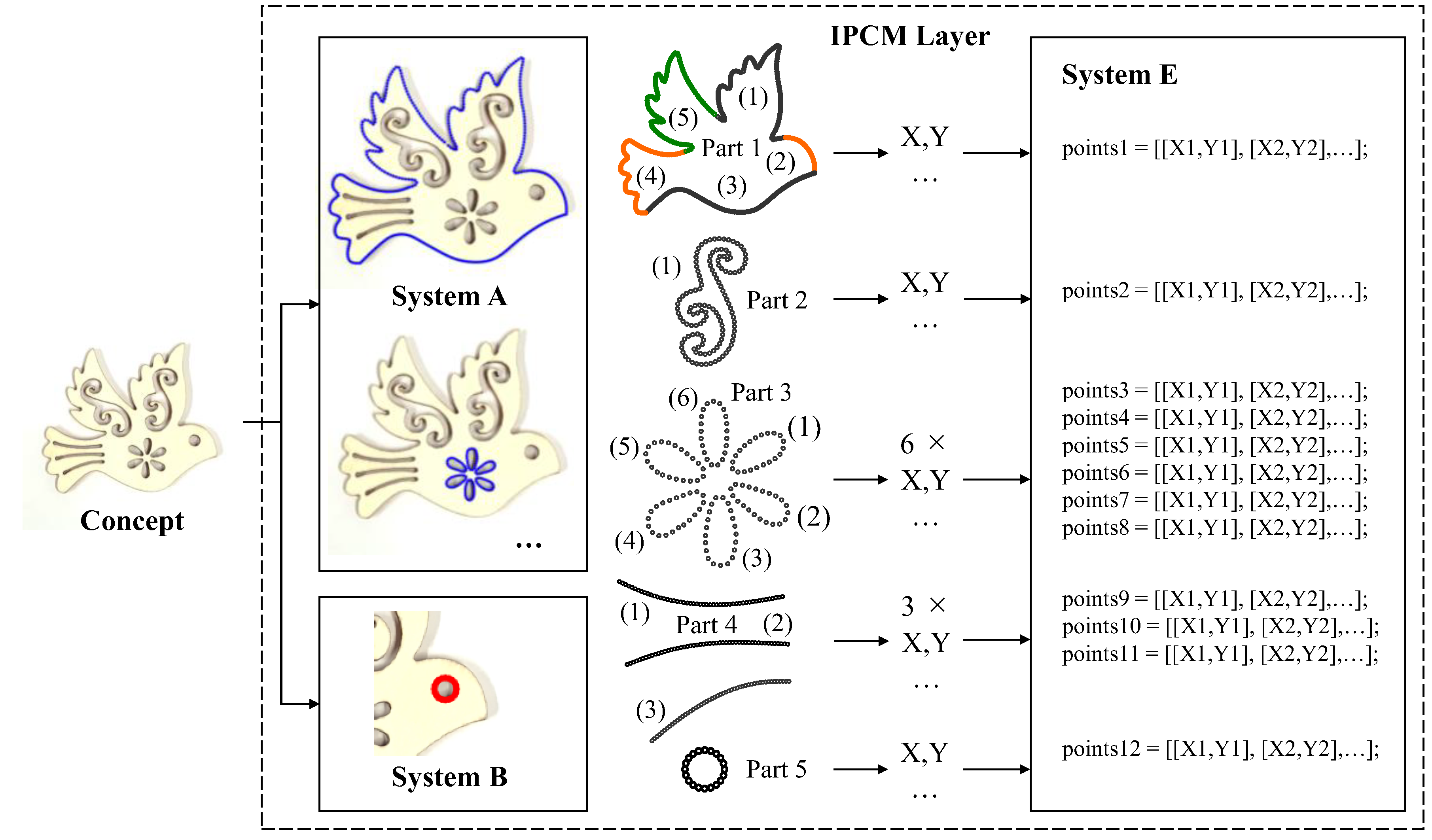
Figure 23.
Rendering and constructing CAD model from the generated points in Figure 22.
Figure 23.
Rendering and constructing CAD model from the generated points in Figure 22.
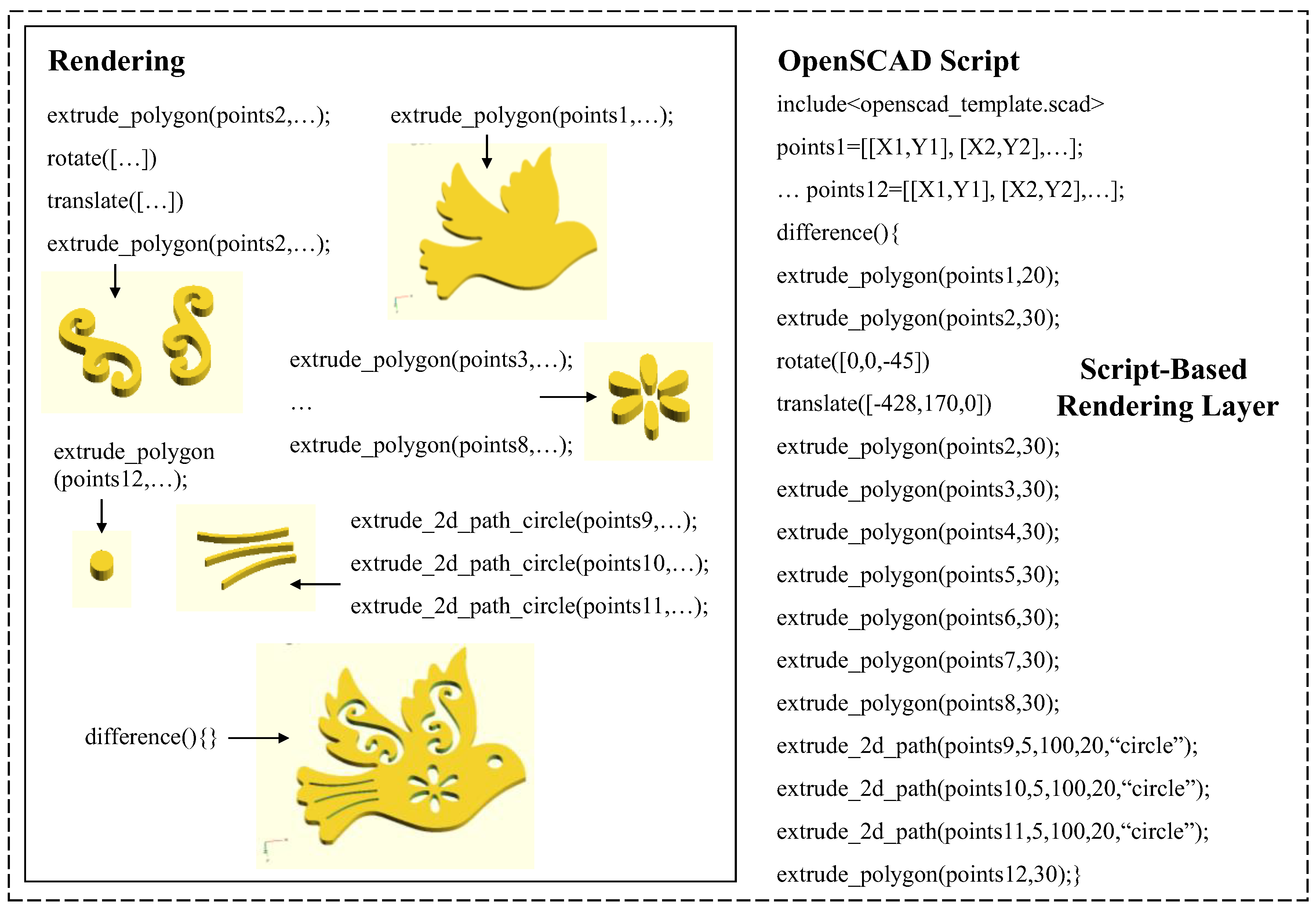
Figure 24.
Generating points in the IPCM layer for a spur gear.
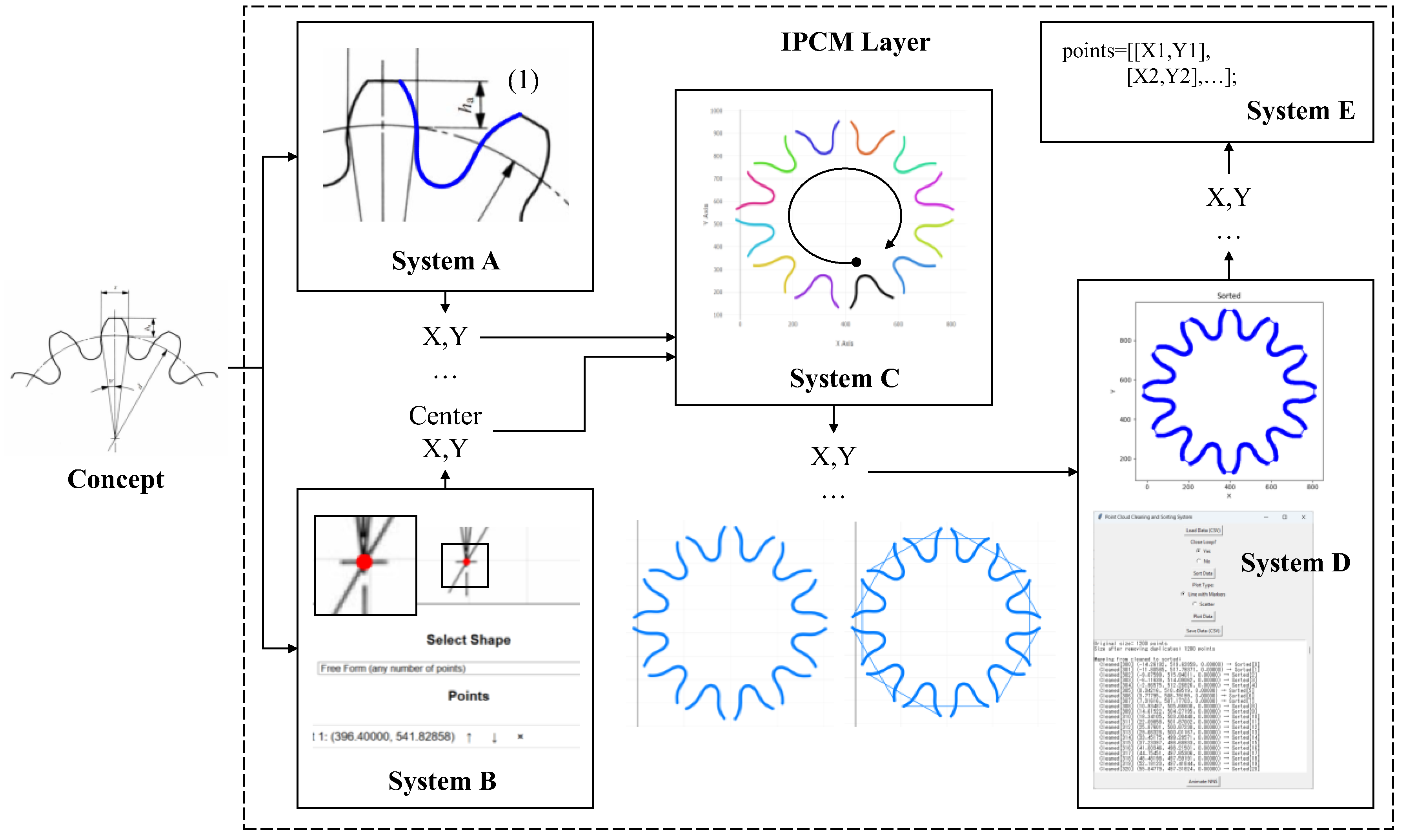
Figure 25.
Rendering and constructing CAD model from the generated points in Figure 24.
Figure 25.
Rendering and constructing CAD model from the generated points in Figure 24.
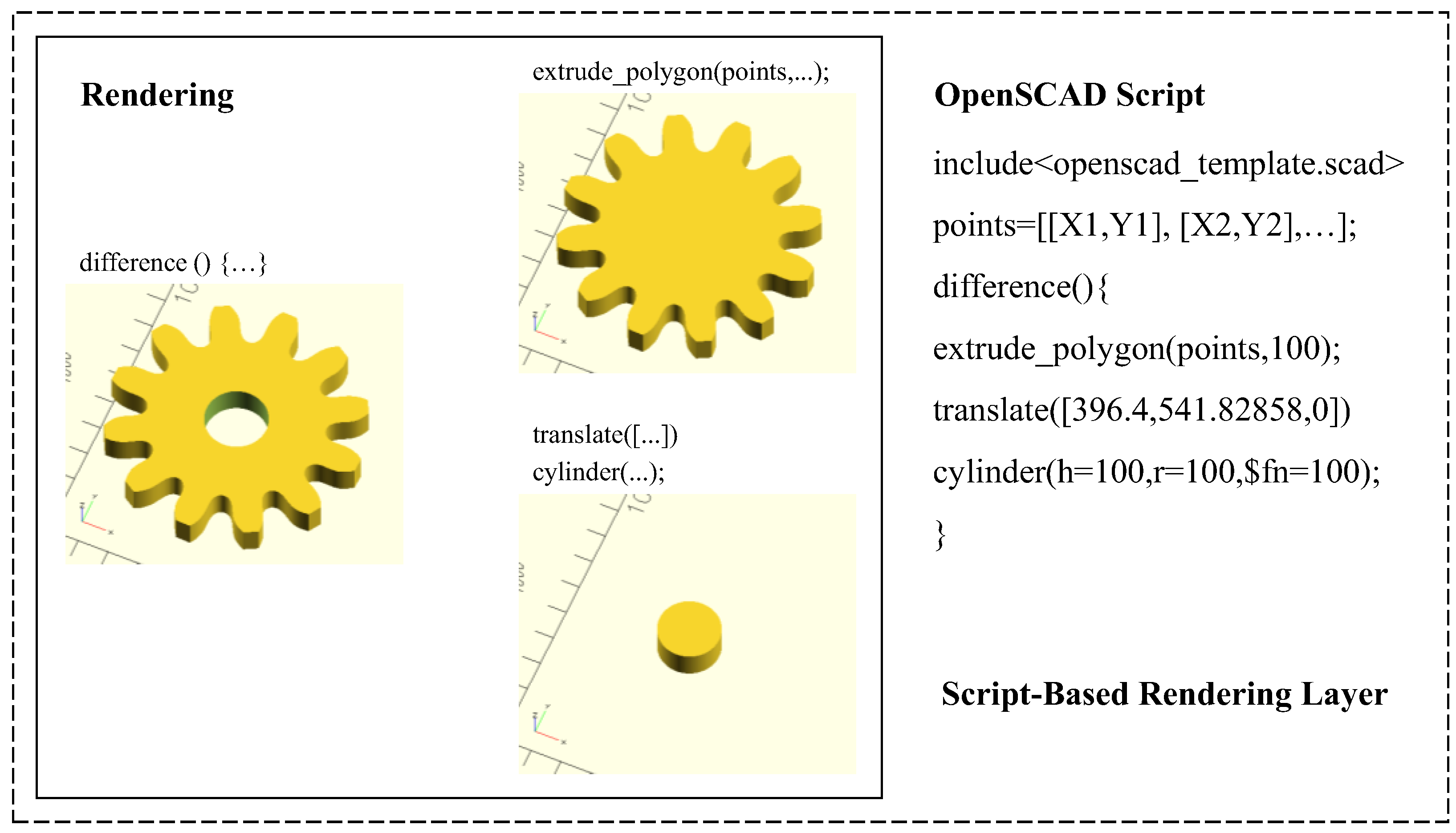
Figure 26.
3D-printed physical prototypes.

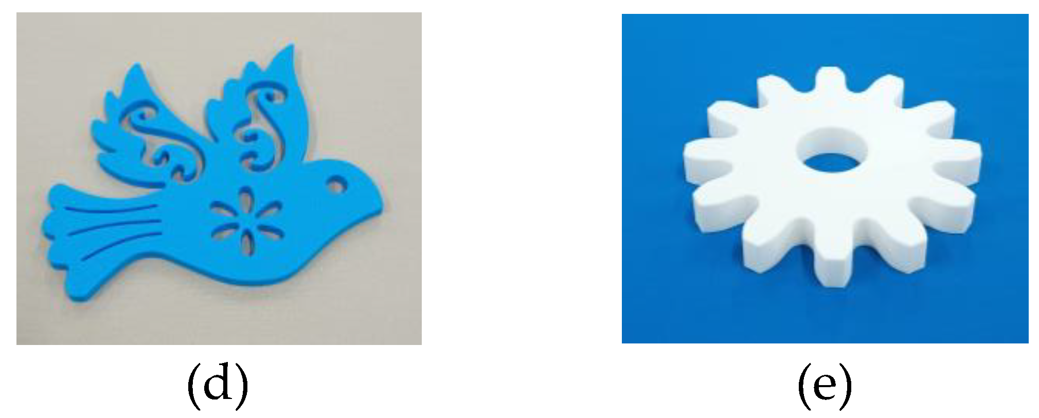
Figure 27.
(a) 2D reconstruction and SVG data, and (b) fabricated samples.
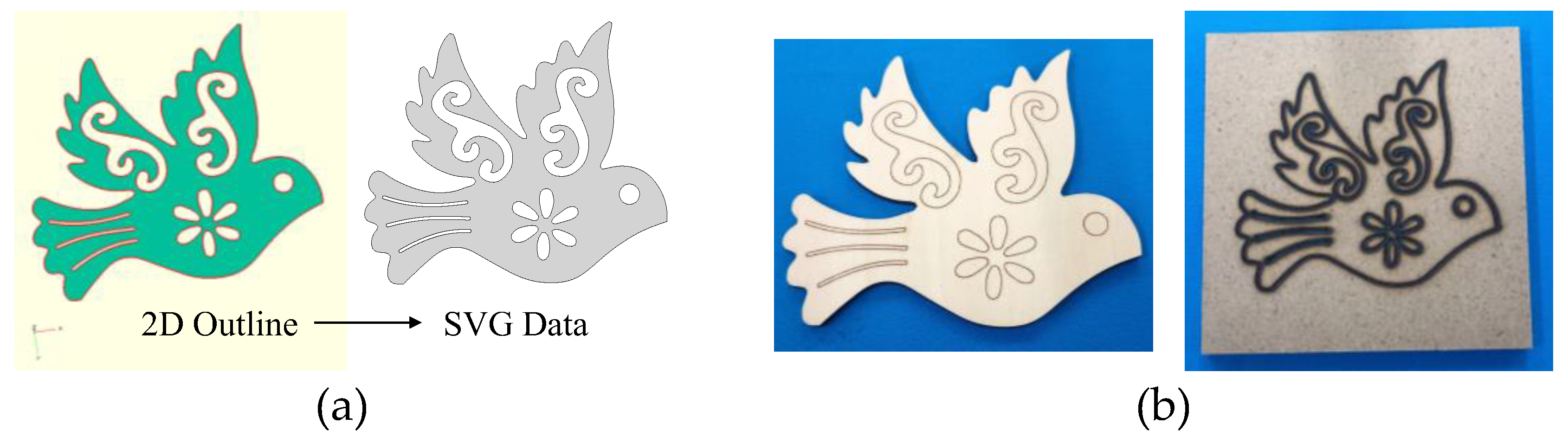
Figure 28.
Alternative rendering of the flower pattern and its 3D-printed counterpart.
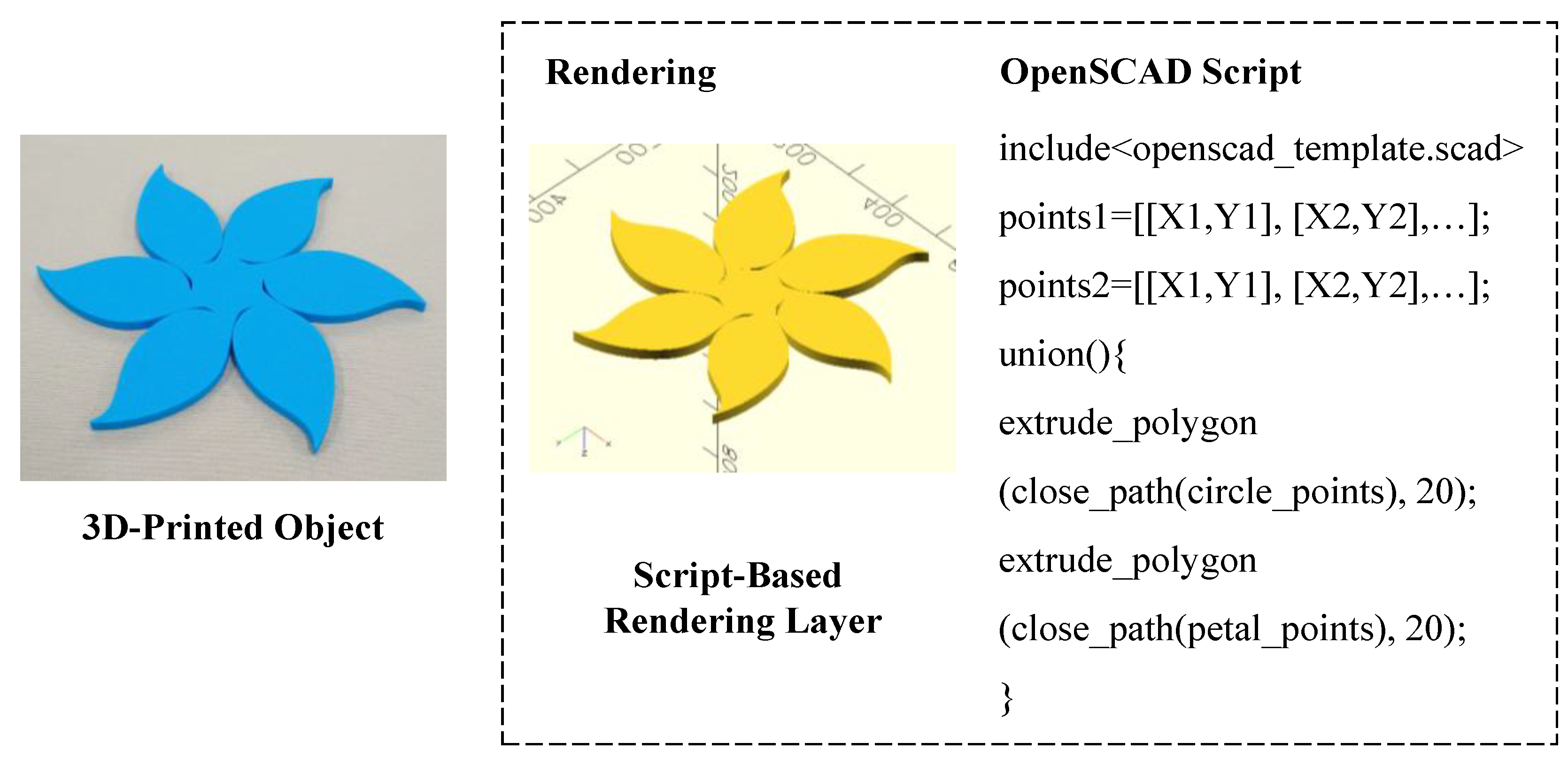
Table 1.
Functional requirements related to the systems in the IPCM Layer.
| Functional Requirements | System A | System B | System C | System D | System E |
|---|---|---|---|---|---|
| User Interface (UI) | ○ | ○ | ○ | ○ | ○ |
| Direct UI Manipulation | ○ | ○ | |||
| Indirect UI Manipulation | ○ | ○ | ○ | ○ | ○ |
| Data Importing | ○ | ○ | ○ | ○ | ○ |
| Parametric Curve Evaluation | ○ | ||||
| Geometric Primitive Generation | ○ | ||||
| Piecewise Construction | ○ | ||||
| Piecewise Point Sampling | ○ | ||||
| Piecewise Continuity | ○ | ||||
|
Transformation
(Rotation, Mirror, Scale…) |
○ | ○ | |||
| Cleaning and Sequencing | ○ | ||||
| Data Formatting | ○ | ||||
| Data Exporting | ○ | ○ | ○ | ○ | ○ |
Disclaimer/Publisher’s Note: The statements, opinions and data contained in all publications are solely those of the individual author(s) and contributor(s) and not of MDPI and/or the editor(s). MDPI and/or the editor(s) disclaim responsibility for any injury to people or property resulting from any ideas, methods, instructions or products referred to in the content. |
© 2025 by the authors. Licensee MDPI, Basel, Switzerland. This article is an open access article distributed under the terms and conditions of the Creative Commons Attribution (CC BY) license (http://creativecommons.org/licenses/by/4.0/).
Copyright: This open access article is published under a Creative Commons CC BY 4.0 license, which permit the free download, distribution, and reuse, provided that the author and preprint are cited in any reuse.


