
Submitted:
24 November 2025
Posted:
26 November 2025
You are already at the latest version
Abstract
Bounds for positive definite sets such as attractors of dynamic systems are typically characterized by Lyapunov-like functions. These Lyapunov functions and their time derivatives must satisfy certain definiteness conditions, whose verification usually requires considerable experience. If the system and a Lyapunov-like candidate function are polynomial, the definiteness conditions lead to Boolean combinations of polynomial equations and inequalities with quantifieres that can be formally solved using quantifier elimination. Unfortunately, the known algorithms for quantifier elimination require considerable computing power, meaning that many problems cannot be solved within a reasonable amount of time. In this context, it is particularly important to find a suitable mathematical formulation of the problem. This article develops a method that reduces the expected computational effort required for the necessary verification of definiteness conditions. The approach is illustrated using the example of the Chua system with cubic nonlinearity.
Keywords:
positive invariant sets
; Lyapunov techniques
; quantifier elimination
; Chua’s circuit
1. Introduction
Lyapunov’s direct method enables stability analysis without knowing the explicit solution of a (usually nonlinear) differential equation [1,2]. This method was originally introduced for stability analysis of equilibrium points, but has been extended to numerous related problems in recent decades. In addition to control theory applications, e.g. with control Lyapunov functions, Lyapunov’s method can also be used to estimate basins of attraction, trapping regions and attractors [3,4,5].
If a nonlinear dynamic system has a chaotic attractor, then the geometry of this attractor usually cannot be described exactly in a straightforward manner. For many questions, such as estimating the attractor’s dimension [6,7], it is necessary or helpful to narrow down this attractor in the state space. Such an containment can be realized via positive invariant sets, which are described by sublevel sets of a Lyapunov-like function [3,4,5]. In this case, one starts from a positive definite Lypunov-like candidate function and must show that its time derivative along the dynamic system in question is negative outside the sublevel set. There are two difficulties here: firstly, choosing the correct candidate function, and secondly, showing that its total time derivative is negative for large values. In particular, the second step usually requires extensive experience and intuition.
The positive definiteness of the candidate function can usually be ensured or easily verified. The property that the time derivative of the candidate function is negative in certain regions can be described by combining inequalities with quantifiers. For polynomial systems with a polynomial Lyapunov candidate function, these inequalities are polynomial as well and the resulting formulas with quantifiers can be solved with a technique known as quantifier elimination (QE) [8,9,10,11].
The calculation of bounds for positively invariant sets using QE has already been successfully applied to the Lorenz system, the Lorenz-Haken system, and a system going back to Rössler [12,13]. This approach was successful because the Lyapunov candidate functions used were fairly simple. Minor generalizations of the Lyapunov candidate functions would quickly result in a situation where the required calculations could no longer be performed within a reasonable amount of time. For further applications of the proposed approach, it is therefore important to reduce the computational effort. In [14], a method was developed to simplify the underlying quantifier elimination problem when searching for suitable Lyapunov functions. This method was reduced to the two-dimensional case and focused on stability analysis of equilibrium points. This paper extends the approach to systems of arbitrary finite dimension. In addition to analyzing the stability of equilibrium points, it is also possible to determine bounds for positively invariant sets.
The paper is structured as follows. In Section 2 we provide mathematical preliminaries. The Lorenz system is discussed in Section 3 as a motivational example, where the choice of the Lyapunov-like candidate function has an impact on the computability. The main result is presented in Section 4. In Section 5 we illustrate the approach on Chua’s system with cubic nonlinearity. The results are discussed in Section 6.
2. Mathematical Preliminaries
2.1. Nonlinear Systems and Positive Invariant Sets
Consider a nonlinear autonomous system
of ordinary differential equations with the vector field with the state vector x. For the computational methods derived in the paper we assume that the vector field f is polynomial, i.e., its components are multivariate polynomials in the variables with rational coefficients. From this follows that f is smooth and locally Lipschitz. Consequently, for every initial value there exists an at least locally defined unique solution . The existence of a global solution will become apparent later, when bounds of the solution have been shown.
A subset is called positive invariant with respect to (1) if every solution of (1) starting in stays in for all future times, i.e.,
Such sets are also called trapping regions [15]. Positive invariant sets can be approximated using Lyapunov-like candidate functions and a constant by
where the subset is bounded by the level set . If all solutions of (1) starting with initial values with tend to , the set contains an attractor. In this case, the solution of (1) is bounded by
Without explicit knowledge of the solution of (1), the bound describing the subset (3) can be computed by
using Lyapunov techniques, where the derivative is the directional derivative of V along the dynamics of system (1). This derivative can be written as a Lie derivative of the scalar field V along the vector field f, i.e.,
see [2]. Alternatively, the bound can be calculated using the differential inequality
as suggested in [16]. The result is an interval for , from which the minimum or infimum is selected as the best bound.
Example 1.
Quadratic forms
with a positive definite symmetric matrix are often used as a candidate function for V. When the matrix P contains free parameters, the definiteness can be ensured. For example, by Sylvester’s criterion or a Cholesky decomposition [17,18,19]. A construction method for more general candidate functions is based on sum of squares (SOS) decomposition [20], but leads to a purely numerical procedure. However, it is much more difficult to solve (5) or (7) for the bound γ. In particular, formulas (5) or (7) are only solvable if for large .
2.2. Quantifier Elimination
The formulas (5) and (7) specify the bound for the positive invariant set (3). These formulas contain quantifiers, namely the universal quantifier ∀ and the existential quantifier ∃. These formulas can be solved by quantifier elimination.
Let us briefly introduce some notations and concepts [9]. The starting point for our considerations are polynomial equations or inequalities over the reals of the form
called atomic formulas in the variables . A Boolean combination of finitely many atomic formulas using logical operators such as is called a quantifier-free formula. A quantifier-free formula describes a semi-algebraic set. Let be a quantifier-free formula in the variables X and the additional variables . A prenex formula has the form
with quantifiers . The variables Y are called quantified variables. The remaining variables not bound by a quantifier are called free variables. The Tarski-Seidenberg theorem [8,9,21] states, that for every prenex formula there exists an equivalent quantifier-free formula solely depending on the free variables X. This transformation from a prenex formula to an equivalent quantifier-free formula is called quantifier elimination (QE).
Over the past half-century, a number of different methods for performing quantifier elimination have been developed. The best-known methods are the cylindrical algebraic decomposition (CAD) [22,23], the virtual substitution (VS) [24,25] and the real root classification [26]. However, all these methods are very computationally intensive. In order to apply QE to practical problems, it is very important to find an appropriate mathematical formulation.
Several software packages are available for solving non-trivial QE problems. The open source package QEPCAD B [27] uses CAD and is available in the repositories of common Linux distributions. The package REDLOG [28] is based on the computer algebra system REDUCE and contains implementations of CAD as well as VS. The computed quantifier-free expressions can be simplified with SLFQ [29]. Commercial computer algebra systems such as Maple or Mathematica also have procedures and libraries for carrying out QE, e.g. [30,31].
Example 2.
Consider the real biquadratic polynomial
with the parameters p and q. The question of the existence of at least one real root can be described by the following prenex formula
where x is a quantified variable and are free variables. Applying QE to (12) leads to the equivalent quantifier-free formula
Similarly, one can ask under what conditions on the parameters the polynomial only takes positive function values:
Carrying out QE to (14) leads to the equivalent quantifier-free formula
3. Motivational Example
The Lorenz system is one of the most popular nonlinear systems exhibiting chaotic dynamics. The system is governed by the differential equations
with positive parameters . To calculate bounds for the Lorenz attractor, numerous Lyapunov candidate functions were investigated [16,32,33,34]. Two well-known candidate functions were given in [5] and [4, Appendix C]:
The level sets of these functions describe a sphere and an ellipsoid, respectively, both shifted with respect to the -axis. Another common feature is that the coefficients of the monomials and are the same within each equation. If we ignore this commonality for the time being, we can consider the functions (17) and (18) as special cases of the Lyapunov candidate function
with the coefficients and , cf. [12]. The time derivative of along (16) is given by
The free parameters should be chosen so that is possible for large . The cubic term is the one with the highest degree. However, the monomial has an odd degree. This monomial can be both positive and negative for large . However, if we choose , the derivative (20) can become negative for large due to the quadratic terms. This explains the above-mentioned commonality in the candidate functions (17) and (18).
If we now ignore the displacement along the -axis, then (19) represents a special case of a quadratic form (8), where the matrix P is a diagonal matrix. The question arises whether a better bound on the invariant set is possible with a dense matrix
The matrix P is positive definite if and only if
according to Sylvester’s criterion [17,18].
The Lie derivative of (8) with the generic matrix (21) is a polynomial in the variables with total degree 3. The terms with the highest degree are
Since the highest degree is an odd number, the associated monomials
are indefinite w.r.t. their sign for large . If these monomials occur in , the condition for will not be fulfilled. Therefore, the entries of the matrix (21) have to be chosen such that the terms (23) vanish. This is achieved by choosing the coefficients as follows
resulting in the diagonal matrix
with .
Remark 1.
The choice (25) corresponds exactly to the coefficients in (19). This means that the dense matrix (21) does not provide any advantage for evaluating the global attraction of (3), i.e., for the behavior of the system for large . This does not rule out the possibility that a dense matrix P could also have advantages for the more precise determination of bounds for invariant sets for smaller .
Remark 2.
For the candidate Lyapunov functions (17), (18), (19) as well as (8) with (21), bounds γ can theoretically be determined exactly (with reference to the respective candidate function) in finite time by applying QE to the formulas (27) and (31). For the candidate function (17), (18), symbolic expressions for the bound γ as a function of the symbolic parameters can be obtained on a standard PC in a few seconds, whereby case distinctions occur for different parameter ranges [12]. When using the candidate function (19), the situation is different. Neither with symbolic nor with numerically specified system parameters did QE deliver a solution, even after several days of computing time. Only when numerical values were specified for the parameters , thereby creating a decision problem, did QE deliver a result. This also meant that it was not possible to directly verify whether the more general approach (8) with (21) offers any advantages.
Problem 1.
Remark 2 implies that the candidate function must be selected in such a way that, on the one hand, there are enough degrees of freedom to meet the definiteness requirements, but on the other hand, there are not too many free parameters to be able to check these definiteness conditions with QE in reasonable time.
4. Results
Section 4.1 deals with the use of QE to validate the local definiteness of functions, as used in the stability analysis of steady states. For this, Section 4.2 describes a necessary condition that requires significantly less computing power. In this process, the terms of lowest degree of a polynomial are evaluated consecutively. If one proceeds in a similar manner in reverse, starting with terms of the highest degree and working downwards, one obtains conditions for Lyapunov candidate functions that are suitable for estimating positive invariant sets, see Section 4.3.
4.1. Description of Local Positive Definiteness by Prenex Formulas
To formulate the stability conditions, we need the concept of positive definiteness of a Lyapunov candidate function V and negative definiteness or semi-definiteness of its time derivative . The algorithms refer to both V and , so we will use the designation in the following. Since we are dealing with polynomials in this paper, all functions are globally defined and continuously differentiable.
Definition 1.
A function is called locally positive definite or positive definite on a neighborhood around the origin if
If (26) holds on , the function is called globally positive definite.
In the same manner we define positive semi-definite with , negative definite with and negative semi-definite with for all . Clearly, a function W is negative definite (semi-definite) if is positive definite (semi-definite). A function W is called indefinite if the function is neither positive semi-definite nor negative semi-definite, i.e., for every neighborhood there exists two points with and .
We assume that the function W is a multivariate polynomial without a constant term, which ensures . If we characterize the neighborhood with using the maximum norm, the test for a given candidate function W regarding local positive definiteness on can be formulated with the following prenex formula:
If W is fully specified without free parameters, the prenex formula (27) constitutes a decision problem, where QE leads either to true or false. If W contains free parameters (e.g. (8) with a symbolic matrix (21)), QE would result in a quantifier-free formula with conditions on the free parameters. In principle, after applying QE, the prenex formula (27) would provide a conclusive test for positive definiteness or a characterization of the free parameter values required for it. However, it is not clear whether, for a given function, QE can be performed within a reasonable time due to the computational effort involved.
Consider a region of the state space defined by
In this region, the substitution
with defines the mapping
and describes a change of coordinates between and . The Lyapunov candidate function W can be written on in the new coordinates as follows:
The regions describe a decomposition of the state space as depicted in Figure 1 for . Condition (27) can be tested for each region separately using the new coordinates by
for . Note that the prenex formula (31) still has the same number of quantified variables as (27). The restriction to one sector could in some cases lead to a simplification of QE, but on the other hand, the degree of some terms will increase due to the multiplication of and x in (29), which can lead to a higher computational effort.
Remark 3.
If the auxiliary variables are fixed (or assumed to have already been eliminated), then the function is a univariate polynomial in the variable z. The definiteness of a single term of a univariate polynomial can be easily determined. For an even number k, the term is positive or negative definite if and only if or , respectively. For an odd number k, the term with is indefinite. Transforming a multivariate polynomial into a univariate polynomial therefore simplifies the definiteness test.
4.2. Necessary Condition
If the order of consecutive quantified variables of the same quantifier is swapped, the logical statement in question does not change. Changing the order of variables with different quantifiers, on the other hand, changes the statement. Swapping the existential quantifier with the universal quantifier results in the following implication:
Now we apply this implication to (31) and obtain the following necessary condition
with the prenex formula H. The function can be written as a polynomial
in the variable z with coefficients from the ring of real polynomials in . Without loss of generality we assume that the constant term vanishes, i.e., . For fixed values , the prenex formula H simply states the local positive definiteness of the function , i.e., has a local minimum at . For univariate polynomials, this means that the term of lowest degree is even with a positive coefficient. From (33), the formula
is obtained. Formula (35) is therefore a necessary condition for to be locally positive definite. Necessary condition for to be locally negative definite as well as locally positive or negative semi-definite can be formulated similarly.
Remark 4.
For practical implementation, it would be useful to check the various conditions for the coefficients step by step:
If the first condition is fulfilled, then the function is locally positive definite and the algorithm is terminated. Otherwise, the subsequent conditions must be checked.
Remark 5.
Although relation (35) is only necessary for (31), it can be used to restrict the degrees of freedom in the choice of parameters for the Lyapunov candidate function and thus possibly eliminate superfluous terms. From a computational point of view, the formulation (35) has several advantageous compared to (26). On the one hand, the number of quantified variables has been reduced by two. In addition, there is no change between different quantifier types, which is particularly advantageous for performing QE with VS [25]. On the other hand, formulation (35) is based only on polynomials in λ, so that omitting z results in terms of lower degree and thus allows for faster computation.
4.3. Description of Definiteness at Large Values
To check the stability of an equilibrium (typically at the origin), local definiteness conditions must be checked in the neighborhood of this equilibrium. These conditions apply to small values of . For determining bounds for positively invariant sets, however, the behavior for large is of interest. The following form of definiteness is essentially complementary to local definiteness [35].
Definition 2.
A function is called
positive definite at infinity
or
positive definite at large values
if there exists a number with
A function is called (positive) coercive [36] if for .
In a similar way, the terms positive semi-definite, negative definite and negative semi-definite at infinity can be introduced. Clearly, a polynomial coercive function is positive definite at infinity. The use of a coercive function is recommended in itself, since the sets (3) defined by the preimages of such a function are compact.
Example 3.
The function with is positive definite at infinity, but not coercive.
A minor modification of (27) leads to a test of a given candidate function W regarding positive definiteness at infinity with the following prenex formula:
As in Section 4.1, the Lyapunov-like candidate function W can be rewritten on a region according to (30). Then, condition (37) leads to
for . Applying the implication (32) yields the necessary condition
with the prenex formula J. The prenex formula J simply states the positive definiteness of the function at infinity. As before, we consider as an univariate polynomial (34) of degree M in the variable z. For an even degree M, the prenex formula
is a necessary condition for to be positive definite at infinity. For an odd degree M, the prenex formula
is a necessary condition for to be positive definite at infinity.
Remark 6.
As stated in Remark 4, it may be useful for practical implementation to check the conditions on the coefficients step by step. If M is even, the conditions are obtained from (40) as follows:
If the first condition is met, the algorithm can be terminated. Otherwise, the subsequent conditions would need to be examined.
5. Chua’s Circuit with Cubic Nonlinearity
In Section 5.1, we derive a model for Chua’s circuit in which the piecewise-linear nonlinearity is replaced by a cubic polynomial. The conditions for the definiteness of functions at infinity derived in Section 4.3 are applied in Section 5.2 to derive conditions on the structure of a Lyapunov-type candidate function for the Chua system. Admissible ranges for the parameter values of the Lyapunov-like candidate function are determined in Section 5.3. The computation of bounds for the containment of positively invariant sets is performed in Section 5.4.
5.1. System Model
Chua’s circuit is an electronic circuit that can generate a chaotic attractor known as double scroll when appropriate parameter values are used [37,38]. The circuit diagram is shown in Figure 2. Kirchhoff’s circuit laws yields the following differential equations
with and the conductance and . In [37,39], the authors used the normalized parameter values , , and .
The nonlinearity of the circuit is a voltage controlled current source known as Chua’s diode and labeled D in the circuit diagram. Typically, the nonlinearity is a 3-segment piecewise-linear function
In [39], the parameter values and were used. The replacement of the non-smooth function (43) by cubic polynomial
was suggested in [40]. In [41, p. 143], the parameters a and b were chosen such that the functions (43) and (44) assume the smallest distance in the sense of quadratically integrable functions on the interval :
Figure 3 shows both characteristics, which are in very good agreement over the interval , but diverge outside this range.
To illustrate the system’s behavior we carried out a numerical simulation with SageMath [42] using the parameters given above. Using the initial conditions , the transients seem to converge to the chaotic attractor as shown in Figure 4 (left). With the initial conditions , the solution, however, converges towards a limit cycle. This transient response is shown in Figure 4 (right). The axes scalings in Figure 4 show that the limit cycle lies further out in the state space than the chaotic attractor.
5.2. Structure of the Quadratic Lyapunov-like Candidate Function
Consider the Chua system (42) with the cubic nonlinearity (44) and the additional constraints
on the parameters. To derive bounds on a positive invariant set we use a Lyapunov-like candidate function V as a quadratic form (8) with the matrix (21). The function V is positive definite if and only if (22) holds. The positive definiteness of V can thus be easily ensured. The question of whether or how the entries of the matrix P can or should be chosen so that the time derivative becomes negative definite or at least semi-definite for large values is much more difficult.
The time derivative of the Lyapunov-like candidate function V has the form
where the numerator is a multivariate polynomial W in the variables and the parameters. The denominator is a positive constant. The definiteness of can therefore be determined by the definiteness of W. The expression for W is very extensive and is therefore not given here.
Now, we will decompose the state space into three regions as already depicted in Figure 1. Since the vector field f is a polynomial of degree 3 and V is quadratic in the variables , the Lie derivative (6) is a polynomial of degree 4. Therefore, the functions defined by (30) on the three regions are polynomials of the degree 4 in the variable z having the form
with and .
For large , only the terms of degree 4 are relevant. Therefore, the terms of degree 4 should not be positive for all . This corresponds to the property of positive semi-definiteness of at infinity. According to Remark 6 one would therefore check the leading coefficient regarding to its sign first. Together with (46), we therefore obtain the prenex formulas
for similar to (40). The QE was carried out with REDLOG. The resulting quantifier-free expressions were combined using conjunction (AND) and subsequently simplified with SLFQ leading to
Note that if we replace the condition in (49) by the strict inequality , QE would lead to the result .
5.3. Parametrization of the Quadratic Lyapunov-like Candidate Function
Consider the matrix P with the spezial structure according to (51). The matrix P is positive definite if and only if
With the simplification resulting from the structure (51), the numerator polynomial of (47) can be written as
This polynomial function has no terms of degree 3. For the function W to be negative definite at infinity, the monomials , , must have negative coefficients:
These coefficients are negative if
The second order mixed terms could also have an impact on the definiteness:
The calculation of a bound for the delimitation of positively invariant sets would be simplified if these terms could be set to zero. Because of according to (52) the coefficient in (57) cannot become zero. Because after (56), the coefficient in (58) cannot become zero either. The coefficient in (59) becomes zero if and only if
which leads to a further simplification of W:
For we used the parameter values given in Section 5.1. In addition, we normalized . The conditions (52), (56), and (60) lead to
If we add existence quantifiers for and to the expression, then after QE we obtain the condition . For further calculation, we choose . Eliminating yields the condition
on . This means that lies in the (relatively small) interval
For the parameter, we choose the arithmetic mean of the two limits:
With specified, we obtain the condition
on the remaining parameter resulting in
In summary, the following parameters are used for the matrix (51):
5.4. Computation of the Bounds
After specifying the Lyapunov-like candidate function V according to (8) with (51) and (62), an attempt can be made to calculate the bound for a positive invariant set (3). Similar to (7) we use the prenex formula
where only the denominator W of was used to obtain a polynomial formulation (see (47)). Applying QE to (63) should provide conditions for in the form of a quantifier-free formula. Unfortunately, even after several days of computing time, the attempt with QE was unable to deliver a result, so the calculation was aborted.
However, if we replace the symbolic variable with a specific positive number, the prenex formula (63) becomes a decision problem with the possible results true or false, which could be solved on a standard PC in a few hundred milliseconds. In combination with a bisection method, the bound can therefore be calculated with arbitrary precision. Carrying out QE on (63) with yields true whereas yields false. The levels sets of this bound are ellipses shown in Figure 5 with red color. In addition, the transients already depicted in Figure 4 are also shown using blue and green color for the chaotic attractor and the stable limit cycle, respectively. When specifying the elements of the matrix P, arbitrary decisions were also made to determine and . Therefore, other parameter values for the admissible ranges were generated using a random number generator, and we attempted to find a bound using the prenex formula (63). The levels resulting from these bounds are shown with gray color in Figure 5.
6. Discussion
Although the quantifier elimination is a powerful tool to compute definite bounds for attractors, its high computational effort restricts the applicability to rather simple systems and Lyapunov candidates. A slight simplification or reformulation of the problem can reduce the computation time significantly. Therefore, the construction of appropriate quantified formulas is an important topic. In this contribution we have shown a state transformation that is particularly useful for the proof of bounds on positive invariant sets using Lyapunov functions.
By the change of order for the quantifiers necessary conditions for the ansatz parameters can be found much more easily, that is, with less computational effort. Every such reduction for the parameter space in return simplifies the original problem. That the quantifier elimination problem must be solved for each region , separately is of minor importance.
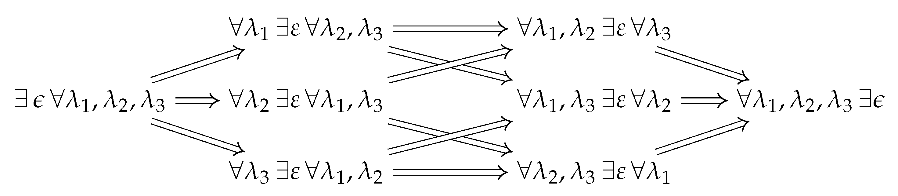
From (31) to (33) or from (38) to (39) the existential quantifier for was swapped several times with the universal quantifiers for . There are a lot of intermediate steps, precisely, one for each partition of the set into two, of gradually changing difficulty that could be considered: Let be disjoint sets such that
Then, according to (32),
Applying this implication to (31) (or (38)) reduces to the problem of positive definiteness (at infinity) in dimension .
All these partitions and implications are shown in Figure 6 for . For the example in Section 5 we have only used the quantified formulas with quantifiers shown on the left corresponding to (38) and on the right corresponding to (39). In general one could get additional restrictions on the parameter space for the Lyapunov candidate function by traversing the graph from the right to the left.
It should be noted that there are in general still a lot of Lyapunov functions that are positive definite (at infinity) with a negative definite (at infinity) derivative along the system dynamics for a particular parametric ansatz. This could also be observed for the example in Section 5. Each of these Lyapunov-like functions yields a positive invariant set, where one candidate function may lead to a better bound than the other. In principle, one could compute the intersection of all these bounds, which is, however, an even more sophisticated semi-algebraic problem.
Author Contributions
Conceptualization, K.R. and D.G.; methodology, D.G.; software, K.R.; validation, K.R.; formal analysis, K.R. and D.G.; writing—original draft preparation, K.R.; writing—review and editing, D.G.; visualization, K.R. and D.G.; project administration, K.R.; funding acquisition, K.R. All authors have read and agreed to the published version of the manuscript.
Funding
This research was funded by the Deutsche Forschungsgemeinschaft (DFG) – 417698841.
Institutional Review Board Statement
Not applicable.
Data Availability Statement
The source files will be available on Github [43] under the GNU General Public License v3.0.
Conflicts of Interest
The authors declare no conflicts of interest.
Abbreviations
The following abbreviations are used in this manuscript:
| QE | quantifier elimination |
| CAD | cylindrical algebraic decomposition |
| VS | virtual substitution |
| SOS | sum of squares |
References
- Slotine, J.J.E.; Li, W. Applied Nonlinear Control; Prentice-Hall: Englewood Cliffs, New Jersey, USA, 1991.
- Khalil, H.K. Nonlinear Control; Pearson: Essex, England, 2015.
- Leonov, G.A.; Bunin, A.I.; Koksch, N. Attractor Localization of the Lorenz System. ZAMM - Journal of Applied Mathematics and Mechanics 1987, 67, 649–656. [CrossRef]
- Sparrow, C. The Lorenz Equations: Birfucations, Chaos, and Strange Atractors; Springer-Verlag: New York, 1982.
- Li, D.; an Lu, J.; Wu, X.; Chen, G. Estimating the bounds for the Lorenz family of chaotic systems. Chaos, Solitons & Fractals 2005, 23, 529–534. [CrossRef]
- Reitmann, V.; Leonov, G.A. Attraktoreingrenzung für nichtlineare Systeme; Vol. 97, Teubner-Texte zur Mathematik, BSB Teubner: Leipzig, 1987.
- Kuznetsov, N.; Reitmann, V. Attractor dimension estimates for dynamical systems: theory and computation; Springer, 2020.
- Tarski, A. A Decision Method for Elementary Algebra and Geometry; Project rand, Rand Corporation, 1948.
- Caviness, B.F.; Johnson, J.R., Eds. Quantifier Elimination and Cylindical Algebraic Decomposition; Springer: Wien, Austria, 1998.
- She, Z.; Xia, B.; Xiao, R.; Zheng, Z. A semi-algebraic approach for asymptotic stability analysis. Nonlinear Analysis: Hybrid Systems 2009, 3, 588–596. [CrossRef]
- Tong, J.; Bajcinca, N. Computation of Feasible Parametric Regions for Common Quadratic Lyapunov Functions. In Proceedings of the European Control Conference (ECC), Limassol, Cyprus, 2018; p. 807–812.
- Röbenack, K.; Voßwinkel, R.; Richter, H. Automatic Generation of Bounds for Polynomial Systems with Application to the Lorenz System. Chaos, Solitons & Fractals 2018, 113C, 25–30. [CrossRef]
- Röbenack, K.; Voßwinkel, R.; Richter, H. Calculating Positive Invariant Sets: A Quantifier Elimination Approach. Journal of Computational and Nonlinear Dynamics 2019, 14. [CrossRef]
- Natkowski, L.; Gerbet, D.; Röbenack, K. On the Systematic Construction of Lyapunov Functions for Polynomial Systems. PAMM 2023, 23, e202200197.
- Pogromsky, A.Y.; Santoboni, G.; Nijmeijer, H. An ultimate bound on the trajectories of the Lorenz system and its applications. Nonlinearity 2003, 16, 1597–1605.
- Krishchenko, A.P. Localization of invariant compact sets of dynamical systems. Differential Equations 2005, 41, 1669–1676.
- Gilbert, G.T. Positive definite matrices and Sylvester’s criterion. The American Mathematical Monthly 1991, 98, 44–46.
- Marcus, M.; Minc, H. A Survey of Matrix Theory and Matrix Inequalities; Dover, 1992.
- Tibken, B.; Dilaver, K.F. Computation of subsets of the domain of attraction for polynomial systems. In Proceedings of the Proceedings of the 41st IEEE Conference on Decision and Control, 2002. IEEE, 2002, Vol. 3, p. 2651–2656.
- Ichihara, H. Sum of Squares Based Input-to-State Stability Analysis of Polynomial Nonlinear Systems. SICE Journal of Control, Measurement, and System Integration 2012, 5, 218–225.
- Seidenberg, A. A New Decision Method for Elementary Algebra. Annals of Mathematics 1954, 60, 365–374. [CrossRef]
- Collins, G.E. Quantifier elimination for real closed fields by cylindrical algebraic decompostion. In Proceedings of the Automata Theory and Formal Languages 2nd GI Conference Kaiserslautern, May 20–23, 1975. Springer, 1975, p. 134–183.
- Collins, G.E.; Hong, H. Partial Cylindrical Algebraic Decomposition for Quantifier Elimination. Journal of Symbolic Computation 1991, 12, 299–328. [CrossRef]
- Weispfenning, V. The complexity of linear problems in fields. Journal of Symbolic Computation 1988, 5, 3–27. [CrossRef]
- Sturm, T. Thirty Years of Virtual Substitution: Foundations, Techniques, Applications. In Proceedings of the Proc. of the 2018 ACM on International Symposium on Symbolic and Algebraic Computation. ACM, 2018, p. 11–16.
- Gonzalez-Vega, L.; Lombardi, H.; Recio, T.; Roy, M.F. Sturm-Habicht Sequence. In Proceedings of the Proc. of the ACM-SIGSAM 1989 International Symposium on Symbolic and Algebraic Computation, Portland, Oregon, USA, 1989; p. 136–146. [CrossRef]
- Brown, C.W. QEPCAD B: A program for computing with semi-algebraic sets using CADs. ACM SIGSAM Bulletin 2003, 37, 97–108. [CrossRef]
- Dolzmann, A.; Sturm, T. Redlog: Computer algebra meets computer logic. ACM SIGSAM Bulletin 1997, 31, 2–9. [CrossRef]
- Brown, C.W.; Gross, C. Efficient preprocessing methods for quantifier elimination. In Proceedings of the CASC. Springer, 2006, Vol. 4194, Lecture Notes in Computer Science, p. 89–100.
- Iwane, H.; Yanami, H.; Anai, H. SyNRAC: A Toolbox for Solving Real Algebraic Constraints. In Proceedings of the Mathematical Software – ICMS 2014; Hong, H.; Yap, C., Eds., Berlin, Heidelberg, 2014; Vol. 8592, Lecture Notes in Computer Science, p. 518–522.
- Chen, C.; Maza, M.M. Quantifier elimination by cylindrical algebraic decomposition based on regular chains. Journal of Symbolic Computation 2016, 75, 74–93.
- Leonov, G.A.; Bunin, A.I.; Koksch, N. Attraktorlokalisierung des Lorenz-Systems. ZAMM – Journal of Applied Mathematics and Mechanics 1987, 67, 649–656. [CrossRef]
- Krishchenko, A.P.; Starkov, K.E. Localization of compact invariant sets of the Lorenz system. Physics Letters A 2006, 353, 383–388. [CrossRef]
- Li, D.; an Lu, J.; Wu, X.; Chen, G. Estimating the ultimate bound and positively invariant set for the Lorenz system and a unified chaotic system. Journal of Mathematical Analysis and Applications 2006, 323, 844–853.
- McCaffrey, D. Geometric existence theory for the control-affine H∞ problem. Journal of mathematical analysis and applications 2006, 324, 682–695.
- Abou-Kandil, H.; Freiling, G.; Ionescu, V.; Jank, G. Symmetric differential Riccati equations: an operator based approach. In Matrix Riccati Equations in Control and Systems Theory; Springer, 2003; p. 411–466.
- Matsumoto, T. A chaotic attractor from Chua’s circuit. IEEE Trans. on Circuits and Systems 1984, 31, 1055–1058.
- Chua, L.O. The genesis of Chua’s circuit. Archiv für Elektronik und Übertragungstechnik (AEÜ) 1992, 46, 250–257.
- Kennedy, M.P. Robust OP AMP realization of Chua’s circuit. Frequenz 1992, 3-4, 66–80.
- Zhong, G.Q. Implementation of Chua’s Circuit with a Cubic Nonlinearity. IEEE Trans. on Circuits and Systems I 1994, 41, 934–941.
- Röbenack, K. Regler- und Beobachterentwurf für nichtlineare Systeme mit Hilfe des Automatischen Differenzierens; Shaker Verlag: Aachen, 2005.
- The Sage Developers. SageMath, the Sage Mathematics Software System (Version 10.2), 2024. https://www.sagemath.org.
- Computation of Bounds for Polynomial Dynamic Systems, Source files. Available online:. https://github.com/TUD-RST/computation-bounds-polynomial-systems.
Figure 1.
Decomposition of the state space.
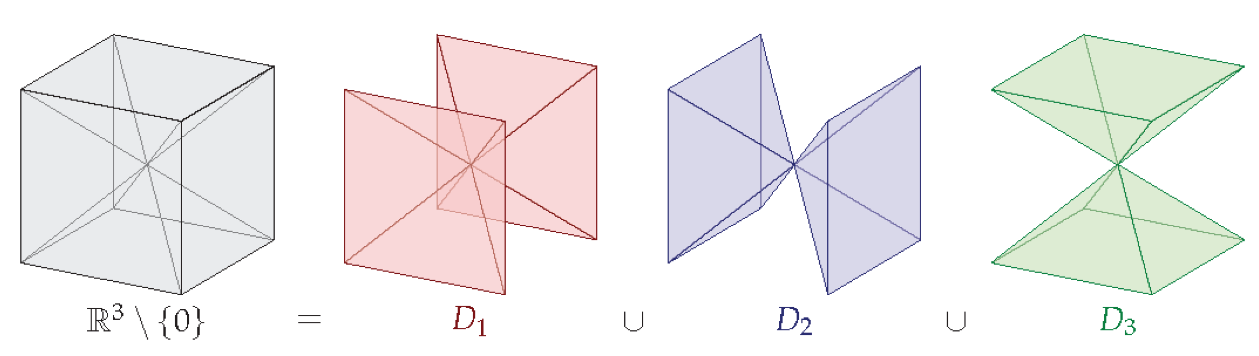
Figure 2.
Circuit diagram of Chua’s circuit
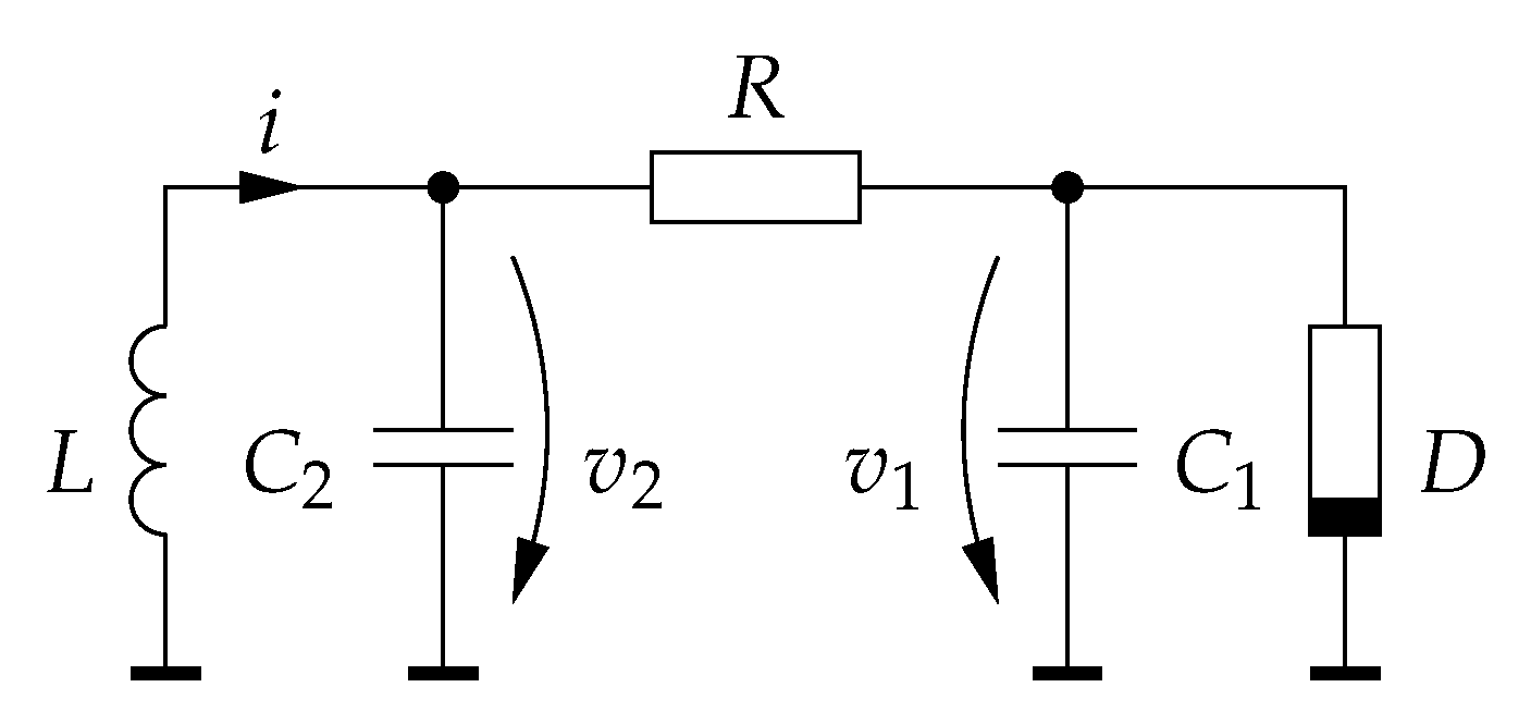
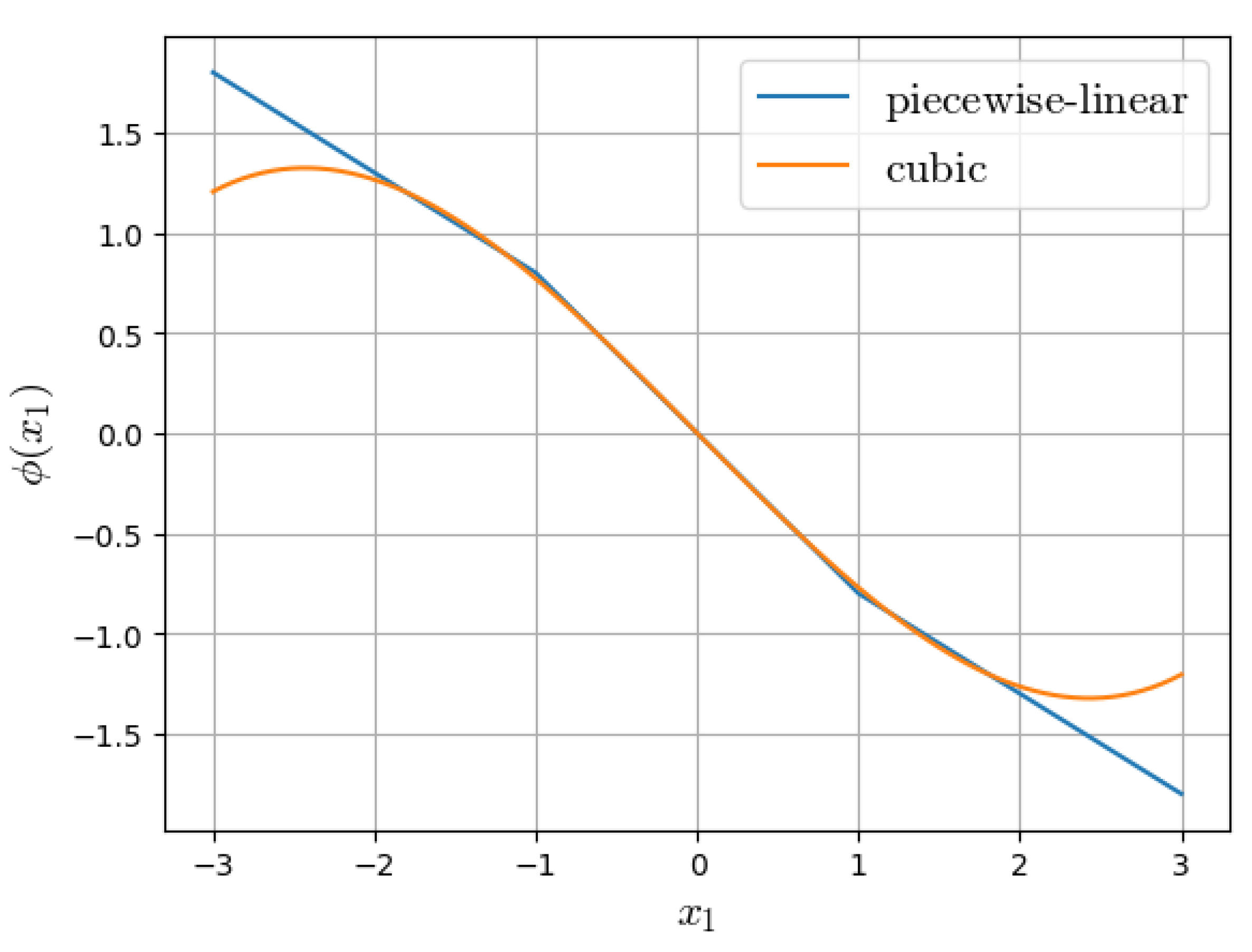
Figure 4.
Numerical simulation results, chaotic attractor (left), settling into a limit cycle (right)
Figure 4.
Numerical simulation results, chaotic attractor (left), settling into a limit cycle (right)
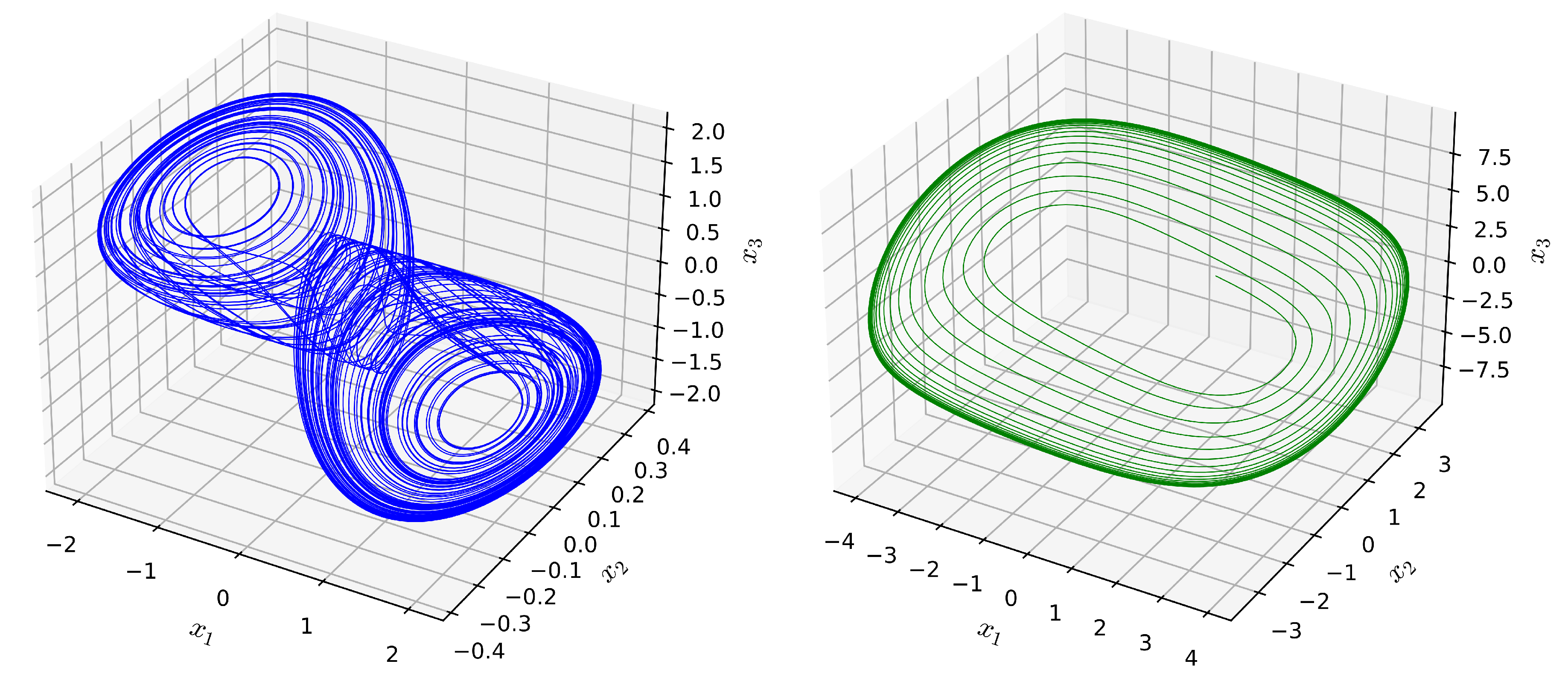
Figure 5.
Bounds on the positive invariant set, projection into the different 2-dimensional planes
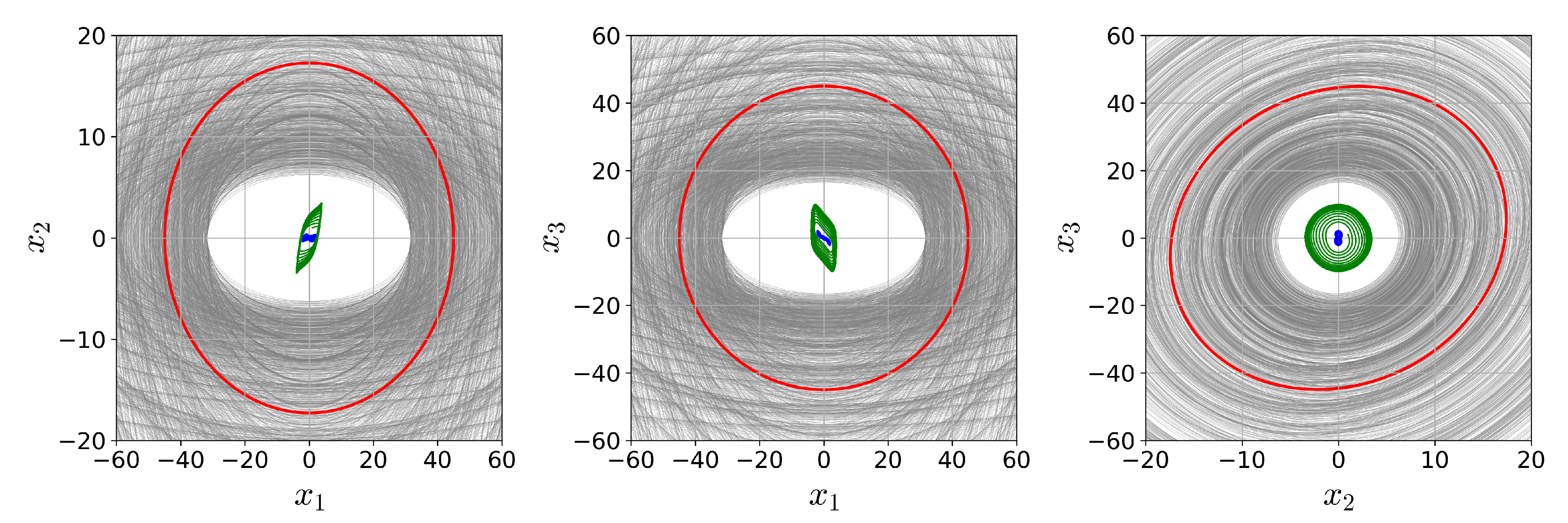
Figure 6.
Swapping the order of quantifiers and the implications of the resulting statements. Shown are all combinations for three universal quantifiers.
Figure 6.
Swapping the order of quantifiers and the implications of the resulting statements. Shown are all combinations for three universal quantifiers.
Disclaimer/Publisher’s Note: The statements, opinions and data contained in all publications are solely those of the individual author(s) and contributor(s) and not of MDPI and/or the editor(s). MDPI and/or the editor(s) disclaim responsibility for any injury to people or property resulting from any ideas, methods, instructions or products referred to in the content. |
© 2025 by the authors. Licensee MDPI, Basel, Switzerland. This article is an open access article distributed under the terms and conditions of the Creative Commons Attribution (CC BY) license (http://creativecommons.org/licenses/by/4.0/).
Copyright: This open access article is published under a Creative Commons CC BY 4.0 license, which permit the free download, distribution, and reuse, provided that the author and preprint are cited in any reuse.


