
Submitted:
21 November 2025
Posted:
25 November 2025
You are already at the latest version
Abstract
This paper presents an analytic and computational framework to study noise in the distribution of prime numbers through layers based on multi-step prime gaps. Given the n-th prime pn, we consider the differences g(k,n) := p(n+k) − p(n), group these distances for different values of k and normalize them by an appropriate logarithmic scale. This produces, for each k, a discrete-time signal that can be analysed with tools from signal processing and control theory (Fourier analysis, resonators, RMS sweeps, and linear combinations). The main conceptual point is that all these layers should inherit the same underlying “noise” coming from the nontrivial zeros of the Riemann zeta function, up to deterministic filtering factors depending on k. We make this idea precise in a heuristic spectral inheritance hypothesis, motivated by the explicit formula and the change of variables t = log x. We then implement the construction computationally for hundreds of thousands of primes and several layers k, and we measure the response of bandpass resonators as a function of their central frequency. The numerical results show three phenomena: (i) the magnitude spectra of the layers share prominent peaks at the same frequencies, (ii) the RMS responses of resonators for different layers display aligned “hills” in the frequency domain, and (iii) a nearly perfect flattening is obtained by taking an appropriate linear combination of layers obtained via singular value decomposition. These findings support the picture that the same spectral content is present across layers and that the differences lie mainly in deterministic gain factors. The framework is deliberately modest from the point of view of number theory: we do not attempt to prove new theorems about primes, but rather to provide a coherent signal- processing view in which standard tools from electrical engineering can be used to explore the noisy side of the prime distribution in a structured way.
Keywords:
prime gaps
; Riemann zeta zeros
; spectral analysis
; signal processing
; FFT
; resonators
; singular value decomposition
; layers of prime gaps
1. Introduction
The distribution of prime numbers encodes deep arithmetic information and has been studied from many perspectives: analytic number theory, probabilistic models, computational experiments, and more recently connections with quantum chaos and random matrices. A central role is played by the Riemann zeta function and its nontrivial zeros; through the explicit formulas, these zeros appear as frequencies in oscillatory terms that correct the main asymptotic behaviour.
From the viewpoint of signal processing, it is natural to interpret these oscillatory terms as a kind of noise superimposed on a smooth trend. This has inspired several approaches where one studies the Fourier transform of arithmetic functions, the response of resonators, or the autocorrelation of prime-related sequences. The present work fits into this general philosophy, but focuses on a specific class of observables based on layers of prime gaps.
Given the sequence of primes , the simplest distance observable is the one-step gap . It is well known that, on average, one has , but the fluctuations around this trend are highly irregular and carry arithmetical information. Instead of looking only at , we consider k–step gaps
for . We refer to the collection for fixed k as the layer of order k. Intuitively, each layer measures aggregated distances between primes over different scales: captures immediate neighbours, looks two steps ahead, and so on.
The central idea of this paper is that, after an appropriate normalization based on logarithms, the fluctuations of these layers should all be driven by the same underlying noise, which in turn is governed by the nontrivial zeros of . The role of k is then to act as a parameter that changes the effective filter applied to this noise, but not the noise itself. This leads to the notion of spectral inheritance: different layers inherit the same spectral content with different deterministic gains.
Our goal is twofold:
- 1.
- To formulate a precise heuristic framework for spectral inheritance based on the explicit formula and the change of variables , which is natural from the point of view of the prime number theorem and its refinements.
- 2.
- To implement this framework computationally and examine the spectral properties of several layers via Fourier transforms and resonator sweeps, with particular attention to the alignment of peaks and the possibility of cancelling the noise by linear combinations of layers.
The rest of the paper is organised as follows. Section 2 recalls the explicit formula for the Chebyshev function and explains how the zeros of appear as frequencies in a variable . Section 3 introduces the definition of layers, their logarithmic normalization and the resulting discrete-time observables. Section 4 describes the spectral inheritance hypothesis and its interpretation in terms of linear systems and frequency responses. Section 5 presents the numerical methodology (grids in t, FFTs, resonators, and RMS sweeps) and the main experimental results. Finally, Section 6 discusses the limitations of the approach and possible extensions.
2. Background: Explicit Formulas and Logarithmic Time
Let denote the Chebyshev function
where the sum runs over prime powers . A fundamental result in analytic number theory is that admits an explicit formula in terms of the zeros of . One convenient form is
where the sum runs over the nontrivial zeros of . For our purposes, the key point is that the terms can be written as
Thus, if we perform the change of variables
the oscillatory terms become exponentials in the variable t. This suggests that it is natural to think of as a signal in the time variable t, whose spectral content is supported at frequencies given by the imaginary parts of the zeros of .
More precisely, if we write
then can be expressed (formally) as a superposition of complex exponentials
plus smoother terms. Thus behaves like a deterministic noise composed of oscillatory modes with frequencies , each modulated by an amplitude factor depending on t and on the real part . If the Riemann hypothesis holds, then for all nontrivial zeros, and the amplitudes decay as .
For our purposes, it suffices to retain the following heuristic picture:
- There is a natural time variable in which prime-related quantities can be viewed as signals.
- The nontrivial zeros of provide characteristic frequencies that appear in the spectral decomposition of these signals.
- The smooth main term corresponds to a trend, and the deviations from this trend can be interpreted as noise with a rich frequency structure.
The layers we introduce in the next section are designed so that their fluctuations can be thought of as measurements of this underlying noise.
3. Layers of Prime Gaps and Logarithmic Normalization
Let be the sequence of prime numbers in increasing order. For each integer , we define the k–step gap
for indices n such that exists in the range of primes we are studying. We call the collection the layer of order k.
Heuristically, one expects to be of size on average, in accordance with the prime number theorem. However, this rule of thumb is not directly suited for spectral analysis, because it does not account for the growth of , and it does not provide a natural time parameter. To address this, we introduce a logarithmic normalization and a time variable as follows.
For each k and n we define
which is the logarithm of the geometric mean of the primes . This choice of time variable has two advantages:
- It centres the measurement of around the primal mass of the block , rather than on a single endpoint.
- It ensures that, when k is fixed and n varies, the time points are approximately equally spaced with respect to the natural density of primes in the logarithmic scale.
We then normalize by the factor and define the dimensionless fluctuation
If the simple heuristic held exactly at the corresponding logarithmic scale, one would have and hence . Thus measures the relative deviation from the expected average behaviour in a scale-invariant way.
The collection can be viewed as a discrete-time signal for each k, sampled at irregular times . To perform spectral analysis in a consistent way across different values of k, we interpolate these samples on a common uniform grid in t, as described in Section 5.
The layer index k plays a role analogous to a scale parameter in multiresolution analysis:
- For , we are looking at immediate neighbour distances between consecutive primes.
- For larger k, we aggregate gaps over longer stretches, which tends to smooth out local irregularities but can enhance the visibility of slower oscillations.
From the viewpoint of spectral inheritance, we expect all layers to be influenced by the same underlying noise, but with different effective frequency responses.
4. Spectral Inheritance and Linear Systems Viewpoint
The explicit formula suggests that many prime-related observables can be expressed, after suitable normalization and change of variables, as linear functionals of the same underlying noise process . Concretely, we imagine a signal of the form
where the sum runs over the imaginary parts of the nontrivial zeros of and are slowly varying amplitudes.
In this picture, our layer signals (obtained from interpolation) are given by
where is an effective kernel that encodes how the layer of order k responds to the underlying noise. This is reminiscent of a linear time-invariant system, although the dependence of on t means that the system is only approximately time-invariant over finite windows.
Taking Fourier transforms in t leads to
where is the frequency response of the k–th layer. If the main spectral content of is concentrated at frequencies corresponding to zeros of , then we expect that:
- The spectra for different k share pronounced peaks at the same frequencies.
- The amplitudes of these peaks differ according to the gain factors .
- Linear combinations of the can be used to enhance or suppress particular frequencies, similarly to the design of filters in electrical engineering.
We refer to this phenomenon as spectral inheritance: the layers inherit the same set of frequencies from the underlying noise, and the differences between layers are captured by deterministic filters.
From a practical standpoint, this viewpoint motivates the following numerical experiments:
- 1.
- Compute the magnitude spectra of several layers via FFT on a common time grid and look for aligned peaks.
- 2.
- Drive simple second-order resonators with and measure the root mean square (RMS) output as a function of the resonator centre frequency, looking for aligned “hills”.
- 3.
- Use singular value decomposition (SVD) to search for linear combinations of layers that produce nearly flat responses, indicating cancellation of the inherited noise.
These experiments are described in detail in the next section.
5. Numerical Methodology and Experiments
5.1. Data and Layers
We work with the first N primes , where N is chosen large enough to provide good frequency resolution while keeping the computational cost manageable. In the experiments reported here, we used values of N up to , with most figures based on to facilitate reproducibility.
For each k in a chosen set (typically ), we compute the k–step gaps
the logarithmic times
and the normalized deviations
This yields, for each k, a cloud of points .
Since the are not exactly equally spaced and the ranges of differ slightly with k, we proceed as follows:
- We determine an interval that is common to all considered layers by intersecting their ranges.
- We construct a uniform grid for with M a power of two (to facilitate FFT).
- For each k, we interpolate onto using simple linear interpolation, obtaining a sampled signal on the common grid.
The choice of M controls the frequency resolution; in the figures, we typically take or .
5.2. Spectral Estimation via FFT
Given a sampled signal on the grid , we subtract its empirical mean to focus on fluctuations and apply a Hann window to reduce spectral leakage:
where . We then compute the discrete Fourier transform
with frequencies for .
In practice, we use the real-to-complex FFT provided by standard libraries and retain only the nonnegative frequencies. The magnitude spectrum is given by , and we interpret as a discrete approximation to the frequency response of the k–th layer.
Figure 1 shows the magnitude spectra for up to a certain cutoff in , highlighting the presence of common peaks.
5.3. Resonator Sweeps and RMS Response
While FFTs provide a global view of the spectral content, it is also informative to probe the layers with simple bandpass filters and measure their output energy as a function of the central frequency. This is analogous to sweeping a resonator across frequencies and monitoring its RMS response.
We consider a family of discrete-time second-order resonators parameterised by a central frequency and a damping factor . A simple model is given by the difference equation
where is the input signal (in our case, ) and is the output. For each in a chosen range, we iterate this filter and compute the RMS value of after discarding an initial transient:
This procedure yields, for each layer k, a function that indicates how strongly the layer excites the resonator at each frequency. If the underlying noise has peaks at frequencies , we expect the RMS curves for different layers to exhibit bumps or “hills” centred near these frequencies.
Figure 2 shows the RMS sweeps for over a range of . The curves share several aligned features, with overall amplitude decreasing as k increases.
5.4. Difference of Layers and Near-Flat Linear Combinations
To probe the coherence of the inherited noise across layers, we consider two related constructions.
First, we examine the simple difference of RMS responses between layers, for instance
If the layers inherit the same spectral content with different amplitudes, we expect to exhibit a smoother profile than the individual RMS curves, although not perfectly flat because of amplitude mismatches and residual differences.
Figure 3 shows , , and their difference . The difference curve has significantly reduced amplitude compared to the individual RMS curves, indicating partial cancellation of the common noise.
Second, we search for linear combinations of RMS curves that are as flat as possible. Concretely, let K be the number of layers considered, and let X denote the matrix whose columns are the sampled RMS curves over L frequency points. We then look for a vector of coefficients such that is nearly constant (or nearly zero) as a function of .
A convenient way to implement this is via singular value decomposition (SVD) applied to the centred matrix
where is the vector of column means and is a vector of ones. The right singular vector corresponding to the smallest singular value provides a candidate coefficient vector that minimizes the variance of .
Figure 4 shows one such almost-flat combination obtained from four layers. The resulting curve is very close to zero across the explored frequency range, providing strong evidence that the layers share a common spectral structure that can be cancelled by an appropriate linear combination.
5.5. Summary of Numerical Steps
For clarity and reproducibility, we summarise here the main steps of the numerical pipeline as pseudocode.
In the final version of the paper we plan to include a code repository (e.g. on GitHub) with the scripts used.
Basic pseudocode.
To compare observed spectral peaks with the imaginary parts of zeros of , we proceed as follows:
- 1.
- Estimate the position of the main spectral peaks (e.g. via local parabolic interpolation around the discrete maximum).
- 2.
- Record the observed frequency .
- 3.
- Compare it with a known zero and compute the relative error
For primes and layers , the most prominent peaks of the spectra in the range appear at frequencies and . When these values are compared with the imaginary parts of the first nontrivial zeros of , we obtain the correspondence shown in Table 1. The relative errors lie between and , which is compatible with the finite-length resolution of the window in t and the discretization of the frequency grid.
This quantitative agreement is consistent with the qualitative picture of Section 2: the layer observables act as linear functionals of the same underlying noise , and therefore they inherit the same set of frequencies . What changes from one layer to another are the filtering factors (determined by the corresponding windows), which modulate the amplitudes but do not create new frequencies. These peaks occur in the same bands where Figure 1 and Figure 2 display the most pronounced structures, reinforcing the interpretation of a common background spectrum shared by all layers.
5.6. Resonator sweeps by layer
The sweeps for share the following features:
- A pronounced maximum at low frequencies (for instance around ).
- “Hills” or bumps in intervals of that align across layers.
- Relative amplitudes that decrease with k, roughly in a way compatible with the normalisation by .
These observations are consistent with the interpretation that all layers inherit the same spectral content with different gain factors.
6. Discussion and Outlook
The experiments reported here support the spectral inheritance picture for layers of prime gaps. The magnitude spectra of the normalized deviations exhibit common peaks at frequencies compatible with the imaginary parts of nontrivial zeros of . The resonator sweeps show aligned hills across layers and a clear decrease of overall amplitude with k. The construction of nearly flat linear combinations via SVD provides a striking visual confirmation that the layers share a coherent noise component that can be cancelled.
From the standpoint of number theory, these findings are heuristic and do not prove new theorems about primes. However, they offer a structured way to view the noisy part of prime distributions through the lens of linear systems and signal processing. Several directions for further work suggest themselves:
- Refining the normalisation and time parameter to better match rigorous asymptotics from the explicit formula.
- Extending the analysis to other arithmetic sequences, such as prime pairs, prime k–tuples, or values of in short intervals.
- Designing resonators tuned to specific hypothetical zeros and studying how the RMS response changes under perturbations of the zero set.
- Exploring connections with random matrix models by comparing the empirical spectra of layers with those of suitable ensembles.
More broadly, the methodology illustrates how a toolbox from electrical engineering—Fourier analysis, windowing, resonators, RMS measurements, and SVD—can be fruitfully applied to classical problems in analytic number theory. Even if the ultimate questions (such as the Riemann hypothesis) remain out of reach, such interdisciplinary views can provide new intuitions and suggest novel quantitative conjectures.
Acknowledgments
The author thanks the mathematical and engineering communities for the many freely available resources (textbooks, lecture notes, software libraries) that make this kind of cross-disciplinary experiment possible.
References
- H. M. Edwards, Riemann’s Zeta Function, Dover Publications, 2001.
- A. Ivić, The Riemann Zeta-Function, Dover Publications, 2003.
- H. L. Montgomery and R. C. Vaughan, Multiplicative Number Theory I: Classical Theory, Cambridge Studies in Advanced Mathematics, Cambridge University Press, 2007.
- A. M. Odlyzko, The 1020-th zero of the Riemann zeta function and 175 million of its neighbors, preprint, available from the author’s webpage.
- T. Tao, Various blog posts on the distribution of primes and the Riemann zeta function, https://terrytao.wordpress.com.
Figure 1.
Magnitude spectra for layers , computed from normalized deviations interpolated onto a common grid in , windowed with a Hann window, and transformed via FFT. The main peaks appear at essentially the same frequencies for all layers, with amplitudes decreasing with k.
Figure 1.
Magnitude spectra for layers , computed from normalized deviations interpolated onto a common grid in , windowed with a Hann window, and transformed via FFT. The main peaks appear at essentially the same frequencies for all layers, with amplitudes decreasing with k.
Figure 2.
Resonator sweeps for layers , obtained by driving a second-order bandpass filter with the windowed signals . The curves share common “hills” at similar values of , while the overall amplitude decreases with k.
Figure 2.
Resonator sweeps for layers , obtained by driving a second-order bandpass filter with the windowed signals . The curves share common “hills” at similar values of , while the overall amplitude decreases with k.
Figure 3.
Resonator sweeps for layers and , and their difference . The difference curve has substantially lower amplitude, reflecting partial cancellation of the inherited spectral content.
Figure 3.
Resonator sweeps for layers and , and their difference . The difference curve has substantially lower amplitude, reflecting partial cancellation of the inherited spectral content.
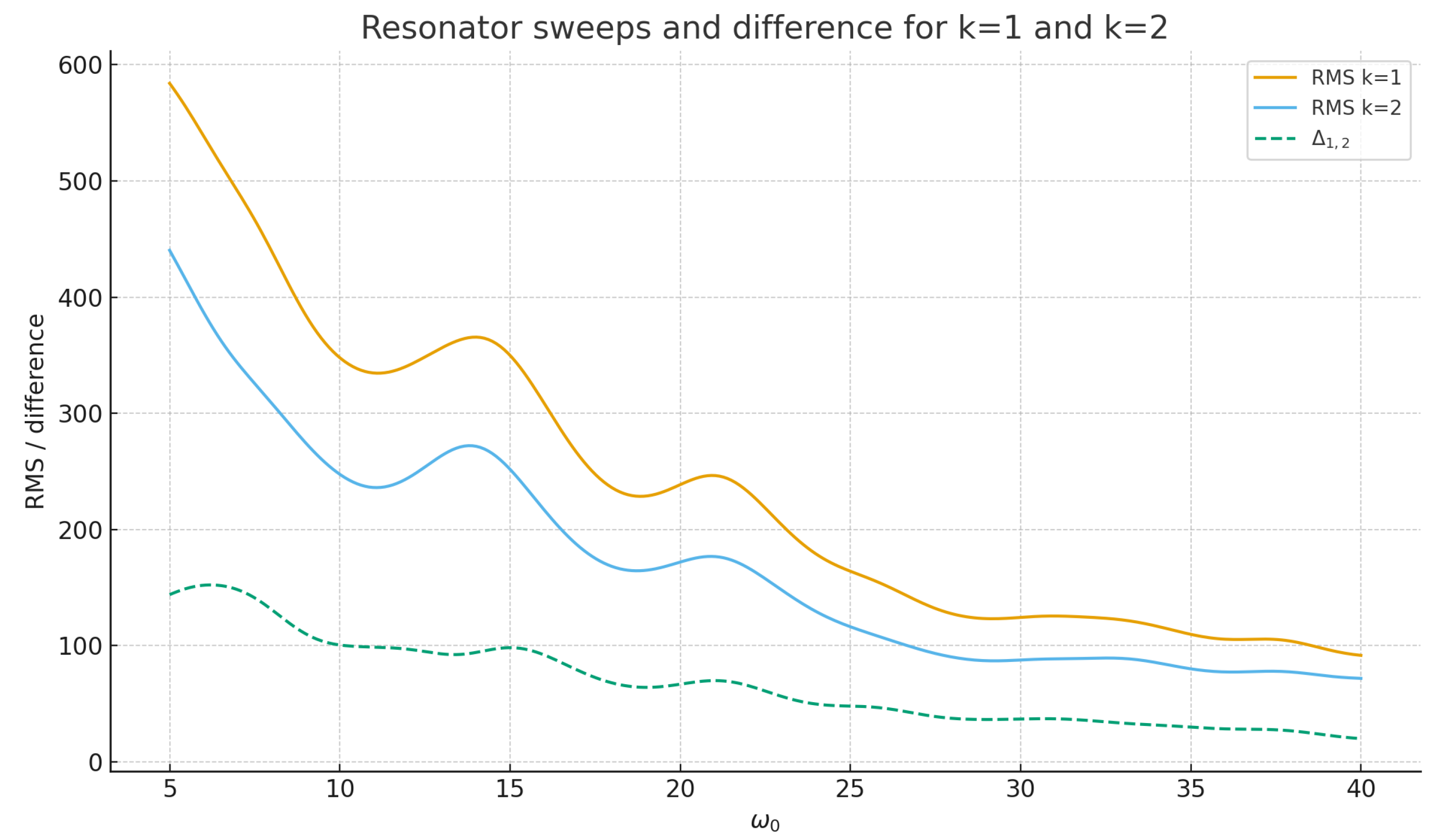
Figure 4.
Resonator sweeps for layers (thin curves) and a nearly flat linear combination (thick curve) obtained via SVD on the centred RMS matrix. The near cancellation supports the idea of a common inherited noise across layers.
Figure 4.
Resonator sweeps for layers (thin curves) and a nearly flat linear combination (thick curve) obtained via SVD on the centred RMS matrix. The near cancellation supports the idea of a common inherited noise across layers.


Table 1.
Correspondence between main observed frequencies in the layer spectra and the imaginary parts of nontrivial zeros of , for primes and grid points in the variable .
Table 1.
Correspondence between main observed frequencies in the layer spectra and the imaginary parts of nontrivial zeros of , for primes and grid points in the variable .
| Peak | Observed frequency | Zeta zero | Relative error |
| 1 | 14.11 | ||
| 2 | 21.16 | ||
| 3 | 33.34 | ||
| 4 | 37.83 |
Disclaimer/Publisher’s Note: The statements, opinions and data contained in all publications are solely those of the individual author(s) and contributor(s) and not of MDPI and/or the editor(s). MDPI and/or the editor(s) disclaim responsibility for any injury to people or property resulting from any ideas, methods, instructions or products referred to in the content. |
© 2025 by the authors. Licensee MDPI, Basel, Switzerland. This article is an open access article distributed under the terms and conditions of the Creative Commons Attribution (CC BY) license (http://creativecommons.org/licenses/by/4.0/).
Copyright: This open access article is published under a Creative Commons CC BY 4.0 license, which permit the free download, distribution, and reuse, provided that the author and preprint are cited in any reuse.


