
Submitted:
22 November 2025
Posted:
25 November 2025
You are already at the latest version
Abstract
Forests play a vital role in the global carbon cycle but face growing anthropogenic pressures, with climate change and forest fragmentation among the most critical. In West Africa, particularly in Ghana, the interaction between increasing aridity and forest fragmentation remains underexplored, despite its significance for forest biomass dy-namics and carbon storage processes. This study examined the effect of climate-driven aridification on above-ground biomass (AGB) in Ghana's ecological zones, both directly and indirectly through forest fragmentation and biodiversity, using structural equation modeling (SEM) and generalized additive models (GAMs). Results from this study show that AGB declines along the aridity gradient, with humid zones supporting the highest biomass and semi-arid zones the lowest. The SEM analysis revealed that areas with a lower aridity index (drier conditions) had significantly lower AGB, indicating that aridification reduces forest biomass. Fragmentation indirectly mediated this effect, while biodiversity (as measured by species richness) showed no significant influence. GAMs highlighted nonlinear fragmentation effects: mean patch area (AREA_MN) was the strongest predictor, showing a unimodal relationship with biomass, whereas number of patches (NP), edge density (ED), and landscape shape index (LSI) reduced AGB. Overall, these findings demonstrate that aridity and spatial configuration jointly control biomass, with fragmentation acting as a key mediator of this relationship. Dry and transitional forests emerge as particularly vulnerable, emphasizing the need for management strategies that maintain large, connected forest patches and integrate restoration into climate adaptation policies.
Keywords:
above-ground biomass
; forest fragmentation
; tropical forest
; remote sensing
; climate change
; aridity index
1. Introduction
Tropical forest ecosystems play a crucial role in regulating the global climate system, acting as significant carbon sinks while supporting biodiversity and maintaining ecosystem functions [1,2]. Among their many ecological contributions, the capacity to store carbon in AGB is critical to mitigating climate change and maintaining ecosystem functions [3]. However, these forests are increasingly threatened by two global drivers: land-use change and climatic variability, which lead to significant changes in biomass dynamics globally [4,5]. In Ghana, these pressures have led to forest degradation, deforestation, and increased fragmentation of forest landscapes [6,7], with a profound impact on woody biomass. Forest fragmentation, a key driver of woody biomass changes, refers to the division of forest landscapes into smaller, isolated patches, decreasing the natural habitat in the landscape [8].
Forest fragmentation results in reduced patch size, increased edge effects, and the isolation of forest fragments, altering microclimatic conditions and disrupting ecological processes, such as species dispersal, gene flow, and nutrient cycling [9,10]. These changes can reduce species richness, alter forest structure, and ultimately diminish. Biodiversity plays a critical role in supporting biomass production, as communities of diverse species can enhance resource-use efficiency, stabilize productivity, and increase resilience to environmental stressors [11]. Thus, biodiversity loss resulting from fragmentation may compound the decline in AGB. Quantifying fragmentation is essential for understanding how landscape structure influences carbon storage dynamics and processes [12]. Most of the fragmentation metrics are strongly correlated, making them redundant if all are chosen for a particular analysis. Selecting a relevant subset from the numerous available metrics can be a challenging task. According to Turner [13], fragmentation metrics must be selected to achieve specific objectives, minimize redundancy, explain pattern variability across the landscape, and encompass a substantial portion of their potential value range. According to Flowers et al. [14], when using fragmentation metrics to quantify landscape structure in forest ecosystems, it is recommended to select metrics that capture the characteristics of the landscape area, edge effects, and shape complexity. Alongside fragmentation, climate change, particularly the decrease in aridity (aridification) and variability in rainfall, has emerged as a critical driver of tropical forest dynamics [15]. Conversion of forests, coupled with climate stress, intensifies fragmentation, reduces biodiversity, and ultimately lowers AGB.
Despite extensive studies on the drivers of AGB in tropical forests in West Africa and Ghana, some critical gaps still remain in literature. Most studies have investigated the direct effects of climate change or forest fragmentation on AGB in isolation, often without considering the interactive effects of these two drivers [16,17]. For example, assessing climate change impacts typically focuses on temperature or precipitation anomalies and their effects on tree growth and mortality [18,19] while those assessing fragmentation tend to concentrate on landscape structural attributes quantified by spatial configuration metrics, such as patch size, edge effects, and landscape connectivity, without considering climatic gradients [10].
This singular approach limits our understanding of how combined environmental conditions jointly influence forest carbon dynamics. In Ghana, existing studies have focused primarily on carbon stock estimation and deforestation monitoring [7,8,9,10,11,12,13,14,15], with a limited focus on how climate stress, such as humidification or aridification, interacts with fragmentation and biodiversity to influence AGB. Several regional studies, primarily conducted in Ghana, have documented relationships between disturbance, biodiversity, and biomass. For example, Oduro et al. [20] and Addo-Fordjour et al. [21] documented declines in woody biomass and species richness with increasing forest disturbance, but without modeling fragmentation metrics or climatic gradients. Similarly, Mensah et al. [22] reported that biodiversity has a positive influence on forest productivity in Ghanaian and Ivorian forest reserves; These relationships were explored independently of spatial configurations or aridity. Only a few studies, such as those by Brinck et al. [23] and Chidumayo and Gumbo [24], have suggested that fragmentation mediates climate-biomass relationships in African drylands; however, extensive quantification and modeling remain scarce. Given Ghana’s climatic gradient from the humid forest zone in the south to the semi-arid savanna zone in the north, it is essential to integrate both climatic and landscape factors when assessing biomass variation. Although climatic stress (e.g., drought and increased temperature) can directly affect biomass, recent findings suggest that its full impact may be amplified or moderated by the degree of forest fragmentation [25]. Thus, the effects of climate change on woody biomass are likely mediated by landscape structure. Yet, these mediating interactions have rarely been explored. Addressing this gap is critical for informing adaptive forest management and carbon conservation strategies. To address these gaps, this study sought to answer the following research questions:
(1) What are the direct and indirect effects of climate change – Aridity Index (AI) on AGB? We hypothesized that decreasing AI (aridification) directly reduces AGB, with wetter zones (higher AI) maintaining higher mean AGB than drier zones. We further hypothesize that decreasing AI (aridification) indirectly influences AGB through its effects on fragmentation and biodiversity.
(2) How do landscape structural attributes, quantified through fragmentation metrics such as number of patches (NP), edge density (ED), mean patch area (AREA_MN), landscape shape index (LSI), and mean shape index (MSI), influence AGB, and what are their relative contributions? We hypothesized that AGB exhibits nonlinear responses to these structural attributes, with varying contributions across different dimensions of fragmentation. Collectively, these questions aim to elucidate the direct and indirect pathways through which climatic aridity, as represented by AI, and landscape structure shape AGB variation across Ghana’s ecological zones.
2. Materials and Methods
2.1. Study Area and Datasets
Ghana is a West African country, bordering Burkina Faso to the north, Togo to the east, Côte d’Ivoire to the west, and the Gulf of Guinea to the south (Figure 1). The geographical coordinates of the country are 7.9465° N and 1.0232° W, and it occupies an area of approximately 238,533 km². Ghana is divided into 16 administrative regions and 261 districts [26]. It has diverse terrain and landscapes, including forests, savannas, mangroves, wetlands, and mountains. Several anthropogenic activities, including agriculture, mining, and logging, have contributed to the degradation of the natural vegetation cover [27]. Almost 15% of its land is protected for conserved species, distinct ecosystems, and ecological processes [28]. The country has a tropical climate, with an average minimum and maximum temperatures of 21 °C and 34.3 °C, respectively [29], and precipitation ranging from 900 to 2000 mm per year, with the highest amounts occurring from April to June in the south and from April to November in the north [30]. This study combined environmental and vegetation variables to assess the relationships between forest fragmentation, biodiversity, and aridity.
2.2. Vegetation Data Extraction
This study employed a data assembly approach in which tree-level occurrence data were obtained from the Global Biodiversity Information Facility (GBIF) website (https://www.gbif.org/) [31]. GBIF is the world’s largest global biodiversity information facility, providing open access to data on all life forms. The network aggregates data from various sources using data standards, including Darwin Core, which forms the bulk of GBIF’s species and tree occurrence records. The data also included field notes and supplementary literature. A targeted search for tree occurrences within Ghana on March 8, 2025, retrieved a total of 38,399 records. The data were subjected to stages of quality control procedures. First, records lacking valid geographic coordinates, scientific names, collection years, duplicates, and points falling outside Ghana’s geographic boundaries were removed.
To eliminate outdated datasets, only occurrences recorded between 2000 and 2011 were retained, resulting in 9,716 valid records. Because GBIF data are known to exhibit strong spatial clustering around well-surveyed areas and regions of higher accessibility [32], a spatial thinning procedure was applied to reduce sampling bias and residual spatial autocorrelation [33]. All occurrences were projected to UTM Zone 30N (EPSG: 32630), and two thinning radii were implemented to generate datasets ready for analysis at different spatial units: a 500m buffer radius, representing fine-scale vegetation distribution patterns, and a 1.5km buffer radius, representing broader landscape-scale heterogeneity. Within each buffer, duplicate coordinates and multiple occurrences of the same species were merged, and a buffer centroid was retained as the representative point.
After thinning, the 500m datasets contained 3,388 records, while the 1.5km dataset contained 2,979 records. To ensure that all tree occurrences represented actual forest tree species, the thinned datasets were subsequently masked using the landcover classification dataset produced by Njomaba et al. [26]. All occurrences falling within landcover classes identified as non-forest were excluded, leaving only points intersecting forest pixels. The final filtered datasets contained 1,211 points for the 500m buffer and 1,067 points for the 1.5km buffers, representing verified forest tree occurrences across Ghana. These were used in subsequent analysis at two spatial levels, representing small and landscape-scale vegetation patterns.
2.2.1. Spatial Autocorrelation Diagnostics
To evaluate residual spatial structure following the spatial thinning procedure, we conducted empirical variograms and Moran’s I correlograms for the GBIF occurrence centroids at 500m and 1.5km spatial data (Figure S1-S2; Table S1). The 500m dataset exhibited a variogram still at ≈ 2.9km and Moran’s I = 0.537 (p = 1.6 x 10 ̶ 195), while the 1.5km dataset leveled at ≈ 3.6km with Moran’s I = 0.337 (p = 2.97 x 10 ̶ 138). Independence (I ≤ 0.05) was not reached within ≤ 6km and ≤ 10km, respectively, indicating moderate residual autocorrelation but sufficient reduction for modeling. These diagnostics validated the choice of thinning radii for the fine- and landscape-level analyses and guided the inclusion of spatial correlation structures in subsequent models.
2.2.2. Biodiversity Metric: Species Richness
In this study, biodiversity was represented using species richness (S), a simple yet widely used computational metric that quantifies the number of unique tree species recorded within a spatial unit. Species richness helps in capturing variations in community composition and is particularly suitable for large-scale biodiversity assessments using occurrence-based data [34]. Tree occurrence records from the cleaned GBIF dataset were first harmonized using the GBIF Backbone Taxonomy through the R package ‘taxize’ [35], ensuring that synonyms and spelling variants were consolidated under accepted species names. Non-tree taxa, duplicates, and occurrences with incomplete taxonomic information were excluded.
After cleaning, richness was computed as the number of distinct tree species within each 500m and 1.5km buffer zones, corresponding to the analytical units described in Section 2.2. Although biodiversity encompasses both computational and structural components, namely species richness and evenness, the computation of evenness metrics, such as Pielou’s J’, requires species abundance that is unavailable in GBIF’s presence-only data. As noted by Meyer et al. [36] and Beck [32], occurrence databases are biased toward collection frequency and survey effort, making abundance metrics unreliable. Therefore, in this study, species richness was used as a robust proxy for local tree diversity, consistent with large-scale studies that rely on presence-only occurrence data [37,38]. While species richness does not fully capture community evenness, it provides an ecologically meaningful and spatially consistent measure of taxonomic diversity across Ghana’s forested landscapes.
2.3. Above-Ground Biomass (AGB) Dataset and Extraction
The AGB data were derived from the European Space Agency (ESA) Climate Change Initiative (CCI) global AGB product (version 5.0.1; [39]). This dataset provides annual estimates of woody AGB (Mg ha-1) at 100m resolution for multiple years (2010 – 2020), oven-dry woody mass of all living trees (stems, branches, twigs, and bark), excluding roots and stumps. Raster layers from 2017 and 2020 were subset to Ghana’s national boundary and resampled to match the analytical grids defined by the 500m and 1.5km GBIF buffer centroids. (Section 2.2). Mean AGB and within-buffer standard deviations (SD) were extracted for each circular buffer, ensuring alignment with spatial predictors (aridity, fragmentation, and biodiversity).
To evaluate the temporal consistency and reliability of the ESA AGB layers, the 2017 and 2020 AGB layers were compared across both spatial resolutions. There is an excellent agreement (r = 0.988) for both scales, with low bias (-0.66 Mg ha-1 at 500m; -0.70 Mg ha-1 at 1.5 km), and small errors (RMSE ≈ 10 Mg ha-1, MAE ≈ 6 Mg ha-1). The mean SD values were 55.4–56 Mg ha-1 across years, confirming stable spatial variability. Based on these diagnostics, the 2020 AGB layer was retained for all analysis as it provides the most recent and spatially complete estimates (Table S2; Figure S3).
2.3.1. Validation of Above-Ground Biomass with GEDI Biomass Footprints
The 2020 ESA CCI AGB layer was validated against the Global Ecosystem Dynamic Investigation (GEDI) Level 2B footprint biomass estimates to assess its accuracy [40]. GEDI provides LiDAR-based estimates of AGB density, derived from waveform structure, representing ~ 25m footprints that directly measure forest vertical structure. GEDI footprints falling within forested areas as defined by the land cover mask described in Section 2.2 were extracted and aggregated to 500m circular buffers to match the AGB spatial scale.
The validated employed both unweighted and uncertainty-weighted metrics, as well as Deming regression (λ = 1) to account for measurement errors in both datasets. The unweighted validation yielded a moderate correlation (r = 0.418; R² = 0.175), with an RMSE of 69.0 Mg ha-1, MAE = 25.9 Mg ha-1, and bias = -0.93 Mg ha-1. Weighted validation improved accuracy (r = 0.200; RMSE = 151.1 Mg ha-1, MAE = 6.48 Mg ha-1 bias = ̶ 6.47 Mg ha-1 ). The Deming regression yielded a slope of (0.40 ± 0.09) and an intercept of (15.25 ± 3.17 Mg ha-1 ), indicating a slight underestimation of higher AGB values but overall strong consistency (Figure S4).
This demonstrates that large-scale spatial gradients in AGB, particularly along aridity and fragmentation axes, reflect genuine ecological variation rather than artifacts of map bias, supporting the use of ESA-CCI AGB for regional modeling. Similar validation approaches using GEDI footprints have demonstrated the robustness of ESA and other satellite-based biomass products across diverse tropical forest contexts [41,42]. The extracted AGB values were assigned to each GBIF buffer centroid. The 500m datasets were used for fine-scale analysis, such as Analysis of Variance (ANOVA) and Principal Component Analysis (PCA). In contrast, the 1.5km dataset was used for the landscape-level analysis (SEMs and GAMs), where reduced spatial dependence among variables is required.
2.4. Climate Data (Aridity Index)
The Global Aridity Index (Global AI) [43] dataset was applied to model the influence of climatic conditions on AGB distribution in Ghana. The dataset provides moderate-resolution (30 arcseconds, ~1 km²) global raster data, characterizing aridity conditions based on the ratio of precipitation to reference evapotranspiration over the period 1970-2000. The data were derived from implementing the Food and Agriculture Organization (FAO)-56 Penman–Monteith Reference Evapotranspiration equation, making it a robust measure of rainfall deficit relative to the atmospheric water demand for vegetation regrowth. The following equation defines the Aridity Index (AI):
These categorical values were used in further analysis to evaluate differences in AGB across climatic gradients. Because Global-AI datasets represent a multidecadal average rather than a single-year climate product, they provide a stable reference for linking long-term aridity conditions to current patterns of biomass, biodiversity, and landscape fragmentation.
2.5. Forest Fragmentation Metrics
Forest structural fragmentation was quantified using the land cover dataset from Njomaba et al. [26], a national land cover map explicitly developed for Ghana. This land cover dataset offers a consistent representation of forest cover and other land cover classes. From this land cover raster, all forest-related land cover classes were reclassified as forest, and all other classes were assigned non-forest. This reclassification produced a binary raster (forest = 1, non-forest = 0), which was used as the base forest mask for fragmentation assessment. To characterize the structure, the binary forest raster was clipped to each of the 500m and 1.5km circular buffers defined in Section 2.2, representing fine and landscape-scale forest patterns, respectively. Within each buffer, five complementary fragmentation metrics were computed using fragmentation statistics (FRAGSTATS) algorithms implemented in the “landscapemetrics” package [45]. The metrics were selected to represent three principal dimensions of forest spatial structure, such as area, edge, and shape complexity, while minimizing redundancy among highly correlated indices.

Table 2.
Forest fragmentation metrics, equations for computation, and their descriptions.
| Fragmentation metrics | Equation | Description |
|---|---|---|
| Number of patches (NP) | Total number of discrete forest patches within the buffer. Higher NP indicates greater fragmentation. |
|
|
Landscape Shape Index (LSI) |
Quantifies shape complexity by standardizing total edge length to landscape area; 0.25 corrects for raster geometry. |
|
| Mean Shape Index (MSI) | Average shape irregularity of forest patches; higher values indicate more complex patch form. |
|
| Edge density (ED) | Total length of forest edges (m) per hectare of landscape area (A). indicates the relative amount of edge habitat. | |
| Mean Patch Area (Area_MN) | Arithmetic means of forest patch areas. Reflects average patch size and connectivity. |
Notes: N = total number of patches, A = total landscape area, eik = total edge length of patch i, aij = area of patch j, m = number of patches, LSI = landscape shape index. All metrics follow landscape ecological equations adopted from McGargical et al. (2012) and Enaruvbe and Atafo. (2018).
2.6. Temporal Consistency and Dataset Alignment
Although the input datasets used in this study span different reference periods (Global AI: 1790 – 2000; GBIF tree occurrences: 2000 – 2013; ESA CCI AGB: 2017 – 2020; land cover, 2023), they were aligned conceptually to represent stable, long-term ecological baselines that reflect persistent climatic, structural, and compositional conditions across Ghana’s forest-savanna transition. The AI represents a long-term climatological average capturing multi-decadal moisture regimes that regulate forest productivity and structure, rather than short-term interannual variability. The ESA CCI AGB dataset provides a recent, yet climatically equilibrated, estimate of woody biomass that integrates vegetation responses to long-term moisture and disturbance gradients. Validation against GEDI footprint biomass confirmed that the ESA CCI AGB products are robust for Ghana (Section 2.2; Figure S4), supporting their use as a baseline for large-scale carbon mapping.
The fragmentation layer, derived from the landcover map of Njomaba et al. [26] for the year 2023. This reflects mid-decade forest structure, consistent with the 2010–2020 period of AGB mapping. Independent assessments by Hansen et al. [47] and Acheampong et al. [48] indicate that national-scale forest loss during this period was gradual and spatially heterogeneous, making the 2023 forest mask representative of prevailing structural conditions. The GBIF biodiversity dataset (2000–2013) aligns temporally with this window and captures distribution patterns shaped by the same underlying climatic and structural drivers.
Together, these datasets represent an ecologically coherent time frame suitable for integrating climate, structure, and diversity within a space-for-time substitution (SFTS) framework [49]. This approach assumes that spatial gradients in aridity and fragmentation substitute for long-term temporal changes, enabling inference on how biodiversity and structure jointly influence carbon storage. All datasets were resampled and aggregated to a common analytical support defined by 500m and 1.5km circular buffers. This ensured that AI, fragmentation, and compositional biodiversity variables were compared over consistent spatial extents. While the original datasets differ in native resolution, the buffer-based extraction effectively harmonized them to a shared spatial support, minimizing the modifiable areal unit problem and scale-dependent variance. To assess robustness, a sensitivity analysis was performed comparing results between 500m and 1.5km datasets for all major analyses, showing a consistent direction and significance of key effects. These consistency checks confirm that the cross-scale patterns reported are not artifacts of resolution or temporal misalignment but reflect stable ecological relationships.
2.7. Temporal Consistency and Dataset Alignment
2.7.1. Effects of Aridity Index on Above-Ground Biomass
To assess the effect of climate change on AGB, we employed an SFTS approach, where spatial variation in aridity, expressed through AI, served as a proxy for temporal climatic change, as described by Blois [49]. Ghana’s four ecological zones (humid, sub-humid, dry sub-humid, and arid) were used to represent increasing levels of aridification, with transitions along this gradient interpreted as analogs of projected climate change impacts.
A one-way ANOVA was conducted to test differences in mean AGB among the four aridity classes. To ensure model robustness, assumptions of normality, homoscedasticity, and independence were evaluated through residual diagnostics. Potential heteroscedasticity was further addressed by applying heteroscedasticity-consistent (HC3) standard errors, implemented through the ‘sandwich’ and ‘lmtest’ packages in R Studio [50]. Post hoc comparisons were performed using the Scheffé multiple comparison test, which is robust to unequal variances and sample sizes [51]. This method was selected based on the approach used in a similar study by Bastias [11], which employed ANOVA to examine vegetation patterns along environmental gradients. Mean and standard deviations of AGB were summarized for each aridity class to describe biomass variation along the climatic gradient.
2.7.2. Multicollinearity and Dimensionality Diagnostics
All predictors were standardized using z-scores before analysis. Multicollinearity among the five fragmentation metrics (NP, ED, AREA_MN, MSI, LSI) was evaluated using pairwise correlation and principal component analysis (PCA). Because these metrics were highly intercorrelated (|r| > 0.8 for ED–LSI and ED-AREA_MN), PCA was applied to reduce redundancy and derive an integrated fragmentation gradient. The first principal component (Frag_PC1) explained the majority of total variance and was used as a component fragmentation variable in subsequent models (Figure S5). After dimensionality reduction, Variance Inflation Factor (VIF) diagnostics were performed on the final set of model predictors to ensure that the combined predictors were not strongly collinear. This two-step approach follows recommended practices for hierarchical ecological modeling [52], where internal collinearity is removed within metric groups with a PCA, and remaining inter-variable collinearity is verified among the final predictors using the variance inflation factor (VIF). All predictors exhibited VIF < 2 and tolerance > 0.8 (Table S4), confirming negligible multicollinearity and validating their inclusion in SEM and GAM analysis.
2.7.3. Structural Equation Modeling (SEM)
To assess the direct and indirect pathways through which AI influences AGB, we implemented both linear and nonlinear SEMs. SEMs were used to jointly estimate causal relationships among AI, fragmentation (Frag_PC1), biodiversity (S), and AGB, while accounting for spatial structures. The linear SEM was implemented using the “piecewiseSEM” package in R Studio, with each sub-model fitted as a generalized least squares (GLS) model that included an exponential spatial correlation structure based on plot centroids (x, y). This approach accounts for residual spatial autocorrelation while preserving parameter estimates. All variables were standardized (z-scores) before modeling to allow comparison of path coefficients (β). The model structure was defined as:
To capture potential nonlinear relationships that the linear model could not represent, a complementary nonlinear SEM was developed using the GAM framework. Each sub-model was fitted using thin-plate regression splines with restricted maximum likelihood (REML) optimization in the “mgcv” package. The structure mirrored the linear SEM but specified smooth functions for key predictors:
2.7.4. Structural Equation Modeling (SEM)
To explore non-linear relationships between AGB and predictor variables, we used spatial GAMs implemented in the “mgcv” package [53]. The main model took the form.
3. Results
3.1. Effects of Aridity on Above-Ground Biomass
Mean AGB declined along the aridity gradient, from the humid to the semi-arid zone (Table 3; Figure 2). A one-way ANOVA showed a highly significant effect of aridity class on AGB (Type–II test: F (3,1201) = 466.64, p < 2.2 x 10 ̶ 16). Effect sizes were large (η² = 0.34, 95% CI 0.31 – 1.00; ω² = 0.34), indicating that approximately one-third of the total variation in biomass was explained by aridity (Table S5). Robust HC3 standard errors confirmed substantially lower AGB in all drier zones relative to humid zones (p < 0.001; Table S6). Scheffé post-hoc comparisons indicated clear differences among aridity zones (Humid > Sub-humid > {Dry sub-humid, Semi-arid}), with the two driest classes not differing statistically (Table S7). The comparison between raw and calibrated AGB showed similar effect sizes (η² = 0.34 vs 0.32), confirming that calibration did not alter the strength of the climatic signal (Table S5). However, mean AGB values were consistently higher in the calibrated dataset (Table S7), which was used in all subsequent analysis.
3.2. Structural Pathways: Linear and Nonlinear SEMs
The linear SEM (GLS-based; n = 1066) captured the main causal pathways linking aridity (AI), fragmentation (Frag_PC1), biodiversity (richness), and above-ground biomass (AGB_cal) (Table 4; Figure 3a). The overall model showed a good fit (Fisher’s C = 3.04, df = 2, p = 0.219), indicating no significant missing paths. The model explained 61.9% of the variance in AGB_cal, 30.4% in fragmentation (Frag_PC1), and 0.4% in richness (Table S8). Aridity (AI) had a strong positive effect on AGB_cal (β = +0.792, p < 0.001), implying that more humid conditions promote higher biomass. In contrast, AI had a negative effect on fragmentation (β = -0.671, p < 0.001), suggesting that drier zones are associated with more fragmented forest structures. Fragmentation, in turn, had a negative effect on AGB (β = -0.223, p < 0.001), indicating that increased fragmentation reduces biomass (Figure 3a, Table S8). The effect of AI on species richness was weak but positive (β = +0.064, p < 0.05), while the path from richness to AGB was non-significant (β = -0.007, p < 0.572).
3.3. Functional Forms of Fragmentation Effects
Spatial GAMs, including individual metrics, confirmed significant nonlinear effects of all five metrics on AGB (edf ≈ 3-7; Table 5). AREA_MN showed the strongest contribution (∆AIC = 386, ∆Dev = 0.043), followed by ED (∆AIC = 268.51, ∆Dev = 0.031), LSI (∆AIC = 256.44, ∆Dev= 0.030), MSI (∆AIC = 156.77, ∆Dev = 0.020), and NP (∆AIC = 71.21, ∆Dev = 0.009). In contrast, biodiversity predictors were not significant (Richness: p = 0.052). Partial effects for the five individual metrics are provided in Figure 4.
4. Discussion
4.1. Aridity as Dominant Driver of Above-Ground Biomass Decline
Our study shows that drier areas support less AGB, with AGB declining systematically from humid to semi-arid zones. Relative to the humid forest, AGB was reduced by ~68% in the sub-humid zone, ~91% in the dry sub-humid zone, and ~97% in the semi-arid zone (Figure 2; Table 3). This supports our hypothesis that decreasing AI (aridification) reduces AGB, which is consistent with the theory and evidence that water availability, shaped by both precipitation and evaporative demand, is a key driver of forest productivity and biomass accumulation [19,20,21,22,23,24,25,26,27,28,29,30,31,32,33,34,35,36,37,38,39,40,41,42,43,44,45,46,47,48,49,50,51,52,53,54,55]. In arid and semi-arid zones, intermittent water availability restricts photosynthesis and plant growth, leading to reduced biomass accumulation [56].
Conversely, humid and sub-humid forests in Ghana benefit from high rainfall and moisture availability, which support high photosynthetic rates, dense forest structures, and elevated carbon storage [57]. Scheffé post hoc tests confirmed that these biomass differences among aridity zones were statistically significant, underscoring that the relationship between aridity and AGB is both systematic and ecologically distinct across moisture regimes. Similar patterns of aridity-driven biomass decline have been observed across tropical regions, including the Amazon Basin, Central Africa, and Northern Australia, where increasing dryness and drought have frequently weakened forest carbon sinks [58,59,60].
These findings reinforce the assertion that the mechanisms driving AGB reduction in Ghana, such as limited water availability and structural degradation, reflect fundamental ecological processes operating throughout the tropics. With climate projections forecasting increased aridification in tropical regions [61], these results have significant implications for forest carbon dynamics.
4.2. Fragmentation as Mediator of Aridity Impacts on Above-Ground Biomass
Our SEM results demonstrated the effect of aridification on biomass not only directly but also indirectly through its influence on fragmentation. Specifically, higher aridity (lower AI) was associated with greater fragmentation, which in turn decreased AGB. Fragmentation (Frag_PC1) captured landscapes dominated by small, irregularly shaped patches with high edge density and shape complexity (NP, ED, LSI positive loadings; AREA_MN and MSI negative loadings). This indicates that drier zones are not only less productive but also structurally more degraded. The mediating role of fragmentation adds an essential layer to understanding carbon dynamics in Ghana’s forest. Numerous studies have demonstrated that fragmentation exacerbates biomass loss beyond that attributable to deforestation alone. By increasing edge exposure, fragmentation accelerates desiccation, tree mortality, and microclimatic stress [62,63]. Patch isolation further disrupts seed dispersal, regeneration, and species persistence, undermining long-term forest stability. In tropical Africa, fragmentation has been linked to reduced carbon storage in both humid forest and savanna-forest mosaics [64,65], consistent with our findings that fragmentation compounds aridity-driven biomass decline.
In Ghana, the dual pressures of climate stress and structural degradation are especially acute in the forest-savanna transition belt, where agricultural expansion (notably cocoa and food crops) has intensified patch proliferation and edge effects [48]. More recently, artisanal mining, known as “galamsey,” and industrial gold mining have emerged as additional drivers of forest fragmentation, converting contiguous forests into small, irregular patches with high edge density, even within protected areas [66,67]. Together, these land-use pressures compound the climatic stress captured in our SEM pathways, reinforcing that fragmentation mediates climate impacts by making forests less resilient to aridification. This interpretation is consistent with evidence showing that fragmented tropical forests are disproportionately vulnerable to climate extremes, such as drought [23], and that structural disturbances, such as selective logging, can lead to long-term carbon losses that further weaken forest resilience [68].
4.3. Limited Role of Biodiversity in Mediating Aridity–Biomass Relationships
Species richness and evenness did not significantly mediate the effects of aridity on AGB in either SEMs or GAMs. This suggests that computational diversity plays a minor role under strong climatic stress. Instead, abiotic drivers (aridification) and structural factors (fragmentation) appeared to dominate biomass dynamics. This outcome is consistent with evidence that biodiversity-biomass relationships are strongly context-dependent, varying in strength and direction depending on climate, resource availability, and structural conditions [69,70,71]. In tropical forests, species richness often enhances biomass through mechanisms such as complementarity and facilitation [70]. However, in dry or transitional ecosystems, biodiversity effects are usually weak or absent because water limitations or structural constraints restrict growth, regardless of species richness [72].
Another possible explanation lies in the biodiversity dataset used. Our species richness measures were derived from occurrence-based GBIF records, which capture species presence rather than abundance. As a result, we could not capture species evenness but only relied on species richness, which is not a great measure of biodiversity. In contrast, above-ground biomass is often disproportionately driven by a few large individuals or dominant species, sometimes referred to as the “big tree effect” [73]. This demographic skew means that biomass and diversity relationships are typically stronger when abundance-weighted diversity metrics, such as basal-area-weighted Shannon or Simpson indices, are available [74,75]. This mismatch between presence-only diversity metrics and abundance-driven biomass likely weakened statistical links in SEM and GAM analysis. Future research could address this limitation by integrating abundance-based forest inventory with remote-sensing products, which could allow more rigorous testing of biodiversity-biomass pathways.
4.4. Functional Responses of Biomass to Fragmentation Metrics
Spatial GAMs provided functional insights into how individual fragmentation metrics influenced AGB across Ghana’s landscape. Among the five metrics, AREA_MN exhibited the most substantial contributions with a unimodal response peaking at intermediate patch sizes. This suggests that moderately sized patches may maximize carbon storage by balancing interior habitat and edge effects, whereas extensive patches reduce AGB. Similar unimodal or hum-shaped relationships between patch size and ecosystem function have been observed in other tropical regions, where moderate fragmentation temporarily enhances heterogeneity before degradation dominates [76,77].
In contrast, the NP showed a negative effect on AGB, particularly at high patch densities. This suggests that excessive patch subdivision reduces the availability of the core forest interior, replacing forest with small, isolated patches that are more exposed to edges. The loss of interior habitat minimizes the capacity of forests to maintain large, biomass-rich trees and heightens vulnerability to disturbances. These findings are consistent with studies from the Amazon and Southeast Asia, where increasing patch number accelerated biomass decline by amplifying fragmentation-driven processes such as edge mortality, drought sensitivity, and fire susceptibility [78,79,80]. For ED, a weak unimodal response was observed. At low to moderate levels of edge creation, biomass appears to increase slightly, which may reflect the role of forest edges in enhancing light penetration and nutrient turnover, thereby stimulating the growth of fast-growing pioneer species [78].
These findings are consistent with studies from the Amazon and Southeast Asia, where increasing patch number accelerates biomass decline by amplifying fragmentation-driven processes, such as edge mortality, drought sensitivity, and fire susceptibility [79,80]. The LSI exhibited a negative relationship with AGB in our models. More regularly shaped patches have larger perimeter-to-area ratios, which expose proportionally greater portions of the forest to edge influences. This reduces the effective area of the forest core, thereby reducing overall biomass [76]. Similar patterns have been documented in both tropical and temperate systems, where complex patch shapes are associated with heightened edge effects, altered species composition, and reduced carbon storage [81,82]. Finally, the mean shape index (MSI) showed the weakest and inconsistent effect from the GAM models for this study.
This suggests that shape connectivity alone may not exert strong control over biomass unless coupled with patch size or edge extent. In other words, irregular shapes may only matter for AGB when patches are fragmented enough that edge effects dominate [83]. Previous studies have shown that patch shape complexity is often a secondary driver of ecological processes compared to patch areas and connectivity [84,85]. Our findings, therefore, highlight MSI as a less robust predictor of biomass compared to AREA_MN, NP, or LSI.
4.5. Functional Responses of Biomass to Fragmentation Metrics
The observed patterns of AGB loss and fragmentation are not only climate-driven but also shaped by long-standing anthropogenic activities. In humid and sub-humid zones, cocoa expansion, oil palm cultivation, and subsistence agriculture remain dominant drivers in Ghana [86]. Cocoa farming has been linked to extensive forest encroachment in Ghana and Côte d’Ivoire, accounting for more than 13% of total forest loss in the region [7]. In drier zones, fuelwood harvesting, charcoal production, and shifting cultivation drive fragmentation and hinder regeneration [24]. Illegal artisanal mining (“galamsey”) has emerged as an additional driver of deforestation and landscape degradation in Ghana, particularly within forest reserves and riparian zones [66,67]. These activities not only remove forest cover but also degrade soil and water resources, compounding fragmentation effects. Weak governance, insecure land tenure systems, and reliance on wood energy (with over 70% of rural households relying on fuelwood and charcoal) [87] further exacerbate patch proliferation and biomass decline. These socio-ecological dynamics compound climatic stress and help explain pronounced AGB reductions observed along Ghana’s aridity gradient.
4.6. Management and Policy Implications Under Climate Change
Our findings carry important implications for forest management and climate policy. Transitional and dry forests, which exhibited the steepest biomass declines, should be prioritized for ecological monitoring and adaptive interventions. While humid forests remain Ghana’s most carbon-rich ecosystems, they are increasingly threatened by fragmentation, induced through climate and anthropogenic activities, requiring policies that maintain large, connected forest patches and minimize edge proliferation. In semi-arid regions, where biomass is inherently low, restoration strategies should emphasize multifunctional land use, such as agroforestry, rather than unrealistic expectations of large carbon sink potential [88].
At the national level, these insights align with the priorities of Ghana’s Forest Plantation Strategy (2018-2021) [89] and the Green Ghana Initiative, both of which emphasize forest restoration and connectivity. However, their effectiveness is increasingly challenged by the activities of illegal artisanal mining, which has become one of the leading drivers of forest degradation and watershed destruction in Ghana [90]. These activities undermine ecosystem recovery and reduce the success of reforestation efforts. Addressing this threat requires integrated strategies that go beyond tree planting, including strict enforcement of mining regulations, community-based monitoring, and the provision of alternative livelihoods [90].
Embedding these measures into national frameworks such as REDD+ and the Green Ghana Initiative will be critical to ensure that gains in forest restoration are not hampered by continuous mining-related degradation. Regionally, Ghana’s experience aligns with the African Forest Restoration Initiative (AFR100), a pan-African effort to restore 100 million hectares of degraded land by 2030. Ghana has pledged to restore 2 million hectares under AFR100 [91], but challenges such as artisanal mining, agricultural expansion, weak governance, and climatic stresses leading to forest fragmentation continue to impede restoration efforts. These findings also align with the goals of the United Nations Decade on Ecosystem Restoration (2021-2030), highlighting that tropical transitional and dry forests are particularly vulnerable to climate change and land-use pressures [92]. These global perspectives underscore the urgency of protecting forest ecosystems and maintaining landscape connectivity across the tropics.
4.7. Limitations and Future Direction
A limitation of this study is the partial temporal mismatch among datasets: the aridity index reflects long-term averages from 1970 to 2000, whereas biomass and vegetation records correspond to 2010, fragmentation (2023), and biodiversity (2000–2013). While the space-for-time substitution framework provides a proxy for assessing climate-biomass relationships, future research should incorporate time-explicit datasets to track ecological and climatic changes directly. Another limitation is the presence of high curvature among smooth terms in the GAMs. Although addressed through PCA-based dimensionality reduction and the inclusion of spatial smoothers, this issue underscores the complexity of disentangling interacting structural variables. Moreover, biodiversity metrics derived from occurrence-based GBIF data may underestimate functional diversity, limiting their exploratory power relative to biomass outcomes. Despite these limitations, SEM and GAM models explained a substantial amount of variance in AGB, demonstrating the combined importance of climatic gradients and landscape structure. Future studies should extend this work by using dynamic modeling approaches that integrate temporal climatic variability, land-use change, and biodiversity composition. Such approaches will strengthen predictions of carbon storage resilience in the face of accelerating aridity and fragmentation pressures.
5. Conclusions
This study demonstrates that aridification (i.e., decreasing AI) is the dominant driver of aboveground biomass variation across Ghana’s ecological zones, with biomass declining sharply from humid to semi-arid forests. The 95% reduction in AGB between these extremes underscores the dominant influence of climatic water availability on controlling forest carbon storage. Aridity effects were compounded by forest fragmentation, which mediated additional biomass losses through reduction in patch size and increase in edge exposure. Spatial GAMs revealed that fragmentation effects were nonlinear: AREA_MN emerged as the strongest predictor, with NP, ED, and LSI contributing secondarily, exhibiting consistently negative effects. MSI was the weakest predictor, suggesting that patch shape complexity alone has little influence without interactions with size or edges.
From a management perspective, these findings emphasize the importance of forest management and conservation. These findings underscore that effective forest management must extend beyond tree cover targets to encompass landscape structural integrity. Conservation and restoration efforts should prioritize dry and transitional forests, maintain large, connected forests, and integrate multifunctional land uses, such as climate-resilient agroforestry, in semi-arid areas. Embedding such strategies into national frameworks, regional efforts, and global agendas will be essential to sustain forest carbon stocks. Our study highlights that protecting moisture-sensitive carbon pools and reducing fragmentation are crucial steps in maintaining the role of tropical forests as a global carbon sink in the face of intensifying climate change.
Supplementary Materials
The following supporting information can be downloaded at the website of this paper posted on Preprints.org.
Author Contributions
Conceptualization, E.N. and P.S.; methodology, E.N.; software, E.N.; validation, P.S. and B.E.A.; formal analysis, E.N.; investigation, E.N.; resources, P..S; data curation, E.N.; writing—original draft preparation, E.N., B.E.A. and P.S; writing—review and editing, E.N., B.E.A. and P.S; visualization, E.N.; supervision, P.S.; project administration, E.N.; funding acquisition, P.S. All authors have read and agreed to the published version of the manuscript. Please turn to the CRediT taxonomy for the term explanation. Authorship must be limited to those who have contributed substantially to the work reported.
Funding
This research was funded by the Faculty of Forestry and Wood Sciences—FFWS, Czech University of Life Sciences Prague, (IGA/FLD/ A_11_23 (grant number: 43140/1312/3189 and grant FORESTin3D) and supported by project TH74010001, funded by the Technological Agency of the Czech Republic through the program Chist-era.
Data Availability Statement
The datasets generated and analyzed for this study are available from the corresponding author upon reasonable request.
Acknowledgments
We extend our profound appreciation to Mr. James Nana Ofori for his pivotal role in ensuring the success of this manuscript. During the preparation of this manuscript/study, the author(s) used [ChatGPT, version 5] for the purposes of [general grammatical checks and correction of sentences]. The authors have reviewed and edited the output and take full responsibility for the content of this publication
Conflicts of Interest
The authors declare no conflicts of interest.
Abbreviations
The following abbreviations are used in this manuscript:
| AGB | Above-ground Biomass |
| AFR100 | African Forest Restoration Initiative |
| AIC | Akaike Information Criterion |
| AI | Aridity Index |
| ANOVA | Analysis of Variance |
| AREA_MN | Mean Patch Area |
| CGLS | Copernicus Global Land Service |
| CGLS-LC100 | Copernicus global land service dynamic land cover map (100m) |
| ED | Edge Density |
| ESA | European Space Agency |
| ESA-CCI | European Space Agency Climate Change Initiative (biomass) |
| ETs | Reference Evapotranspiration |
| FAO | Food and Agriculture Organization |
| GAM | General Additive Model |
| GBIF | Global Biodiversity Information Facility |
| GEE | Google Earth Engine |
| GEDI | Global Ecosystem Dynamics Investigation |
| IPCC | Intergovernmental Panel on Climate Change |
| LSI | Landscape Shape Index |
| MSI | Mean Shape Index |
| NP | Number of Patches |
| NCCP | National Climate Change Policy |
| PCA | Principal Component Analysis |
| REDD+ | Reducing Emissions from Deforestation and Degradation |
| RMSE | Root Mean Square Error |
| SEM | Structural Equation Modeling |
| SFTS | Space for Time Substitution |
| UNEP | United Nations Environmental Programme |
| VIF | Variable Inflation Factor |
References
- Zhang, X.; Huang, X. Human disturbance caused stronger influences on global vegetation change than climate change. PeerJ 2019, 7, e7763. [Google Scholar] [CrossRef]
- Pan, Y.; Birdsey, R.A.; Fang, J.; Houghton, R.; Kauppi, P.E.; Kurz, W.A.; Phillips, O.L.; Shvidenko, A.; Lewis, S.L.; Canadell, J.G.; et al. A Large and Persistent Carbon Sink in the World’s Forests. Science 2011, 333, 988–993. [Google Scholar] [CrossRef]
- Saatchi, S.S.; Harris, N.L.; Brown, S.; Lefsky, M.; Mitchard, E.T.A.; Salas, W.; Zutta, B.R.; Buermann, W.; Lewis, S.L.; Hagen, S.; et al. Benchmark map of forest carbon stocks in tropical regions across three continents. Proc. Natl. Acad. Sci. USA 2011, 108, 9899–9904. [Google Scholar] [CrossRef] [PubMed]
- Tilman, D.; Lehman, C. Human-caused environmental change: Impacts on plant diversity and evolution. Proc. Natl. Acad. Sci. 2001, 98, 5433–5440. [Google Scholar] [CrossRef] [PubMed]
- Bodart, C.; Brink, A.B.; Donnay, F.; Lupi, A.; Mayaux, P.; Achard, F. Continental estimates of forest cover and forest cover changes in the dry ecosystems of Africa between 1990 and 2000. J. Biogeogr. 2013, 40, 1036–1047. [Google Scholar] [CrossRef] [PubMed]
- Asubonteng, K.; Pfeffer, K.; Ros-Tonen, M.; Verbesselt, J.; Baud, I. Effects of Tree-crop Farming on Land-cover Transitions in a Mosaic Landscape in the Eastern Region of Ghana. Environ. Manag. 2018, 62, 529–547. [Google Scholar] [CrossRef]
- Asare, R.; Afari-Sefa, V.; Osei-Owusu, Y.; Pabi, O. Cocoa agroforestry for increasing forest connectivity in a fragmented landscape in Ghana. Agrofor. Syst. 2014, 88, 1143–1156. [Google Scholar] [CrossRef]
- Pyngrope, O.R.; Kumar, M.; Pebam, R.; Singh, S.K.; Kundu, A.; Lal, D. Investigating forest fragmentation through earth observation datasets and metric analysis in the tropical rainforest area. SN Appl. Sci. 2021, 3, 1–17. [Google Scholar] [CrossRef]
- García-Gigorro, S.; Saura, S. Forest Fragmentation Estimated from Remotely Sensed Data: Is Comparison Across Scales Possible? For. Sci. 2005, 51, 51–63. [Google Scholar] [CrossRef]
- Haddad, N.M.; Brudvig, L.A.; Clobert, J.; Davies, K.F.; Gonzalez, A.; Holt, R.D.; Lovejoy, T.E.; Sexton, J.O.; Austin, M.P.; Collins, C.D.; et al. Habitat fragmentation and its lasting impact on Earth’s ecosystems. Sci. Adv. 2015, 1, e1500052. [Google Scholar] [CrossRef]
- Bastias, C.C.; Castilla, G.R.; Zarzosa, P.S.; Herraiz, A.D.; Herranz, N.G.; Ruiz-Benito, P.; Barrón, V.; Pérez, J.L.Q.; Villar, R. Differential aridity-induced variations in ecosystem multifunctionality between Iberian Pinus and Quercus Mediterranean forests. Ecol. Indic. 2025, 173. [Google Scholar] [CrossRef]
- Bonsu, K.; Bonin, O. Assessing landscape fragmentation and its implications for biodiversity conservation in the Greater Accra Metropolitan Area (GAMA) of Ghana. Discov. Environ. 2023, 1, 1–23. [Google Scholar] [CrossRef]
- Turner Monica (1996) Landscape Ecology Theory and Practice. 72–82.
- Flowers, B.; Huang, K.-T.; Aldana, G.O. Analysis of the Habitat Fragmentation of Ecosystems in Belize Using Landscape Metrics. Sustainability 2020, 12, 3024. [Google Scholar] [CrossRef]
- Aabeyir, R.; Adu-Bredu, S.; Agyare, W.A.; Weir, M.J.C. Allometric models for estimating aboveground biomass in the tropical woodlands of Ghana, West Africa. For. Ecosyst. 2020, 7, 1–23. [Google Scholar] [CrossRef]
- Laurance, W.F.; Lovejoy, T.E.; Vasconcelos, H.L.; Bruna, E.M.; Didham, R.K.; Stouffer, P.C.; Gascon, C.; Bierregaard, R.O.; Laurance, S.G.; Sampaio, E. Ecosystem Decay of Amazonian Forest Fragments: a 22-Year Investigation. Conserv. Biol. 2002, 16, 605–618. [Google Scholar] [CrossRef]
- Malhi, Y.; Roberts, J.T.; Betts, R.A.; Killeen, T.J.; Li, W.; Nobre, C.A. Climate Change, Deforestation, and the Fate of the Amazon. Science 2008, 319, 169–172. [Google Scholar] [CrossRef]
- Phillips, O.L.; Aragão, L.E.O.C.; Lewis, S.L.; Fisher, J.B.; Lloyd, J.; López-González, G.; Malhi, Y.; Monteagudo, A.; Peacock, J.; Quesada, C.A.; et al. Drought Sensitivity of the Amazon Rainforest. Science 2009, 323, 1344–1347. [Google Scholar] [CrossRef]
- Clark, D.A.; Piper, S.C.; Keeling, C.D.; Clark, D.B. Tropical rain forest tree growth and atmospheric carbon dynamics linked to interannual temperature variation during 1984–2000. Proc. Natl. Acad. Sci. USA 2003, 100, 5852–5857. [Google Scholar] [CrossRef]
- Oduro, K.; Mohren, G.; Peña-Claros, M.; Kyereh, B.; Arts, B. Tracing forest resource development in Ghana through forest transition pathways. Land Use Policy 2015, 48, 63–72. [Google Scholar] [CrossRef]
- Addo-Fordjour P, Obeng S, Anning A, Addo M (2009) Floristic composition, structure and natural regeneration in a moist semi-deciduous forest following anthropogenic disturbances and plant invasion. Int J Biodivers Conserv 1:21–37.
- Mensah, S.; Veldtman, R.; Assogbadjo, A.E.; Ham, C.; Kakaï, R.G.; Seifert, T. Ecosystem service importance and use vary with socio-environmental factors: A study from household-surveys in local communities of South Africa. Ecosyst. Serv. 2017, 23, 1–8. [Google Scholar] [CrossRef]
- Brinck, K.; Fischer, R.; Groeneveld, J.; Lehmann, S.; De Paula, M.D.; Pütz, S.; Sexton, J.O.; Song, D.; Huth, A. High resolution analysis of tropical forest fragmentation and its impact on the global carbon cycle. Nat. Commun. 2017, 8, 14855. [Google Scholar] [CrossRef]
- Chidumayo E, Gumbo DJ (2010) The dry forests and woodlands of Africa: managing for products and services. Earthscan Libr.
- Chaplin-Kramer, R.; Ramler, I.; Sharp, R.; Haddad, N.M.; Gerber, J.S.; West, P.C.; Mandle, L.; Engstrom, P.; Baccini, A.; Sim, S.; et al. Degradation in carbon stocks near tropical forest edges. Nat. Commun. 2015, 6, 10158. [Google Scholar] [CrossRef] [PubMed]
- Njomaba, E.; Mushtaq, F.; Nagbija, R.K.; Yakalim, S.; Aikins, B.E.; Surovy, P. Adopting Land Cover Standards for Sustainable Development in Ghana: Challenges and Opportunities. Land 2025, 14, 550. [Google Scholar] [CrossRef]
- Ampim, P.A.Y.; Ogbe, M.; Obeng, E.; Akley, E.K.; MacCarthy, D.S. Land Cover Changes in Ghana over the Past 24 Years. Sustainability 2021, 13, 4951. [Google Scholar] [CrossRef]
- Lawer, E.A. Predicting the impact of climate change on the potential distribution of a critically endangered avian scavenger, Hooded Vulture Necrosyrtes monachus, in Ghana. Glob. Ecol. Conserv. 2024, 49, e02804–e02804. [Google Scholar] [CrossRef]
- Ofori, S.A.; Asante, F.; Boateng, T.A.B.; Dahdouh-Guebas, F. The composition, distribution, and socio-economic dimensions of Ghana's mangrove ecosystems. J. Environ. Manag. 2023, 345, 118622. [Google Scholar] [CrossRef]
- Abbam, T.; Johnson, F.A.; Dash, J.; Padmadas, S.S. Spatiotemporal Variations in Rainfall and Temperature in Ghana Over the Twentieth Century, 1900–2014. Earth Space Sci. 2018, 5, 120–132. [Google Scholar] [CrossRef]
- Asare (2021) Plants of Ghana. Version 1.1. In: Ghana Herb. Occur. dataset. [CrossRef]
- Beck, J.; Böller, M.; Erhardt, A.; Schwanghart, W. Spatial bias in the GBIF database and its effect on modeling species' geographic distributions. Ecol. Informatics 2014, 19, 10–15. [Google Scholar] [CrossRef]
- Aiello-Lammens, M.E.; Boria, R.A.; Radosavljevic, A.; Vilela, B.; Anderson, R.P. spThin: an R package for spatial thinning of species occurrence records for use in ecological niche models. Ecography 2015, 38, 541–545. [Google Scholar] [CrossRef]
- Hillebrand, H.; Bennett, D.M.; Cadotte, M.W. Consequences of dominance: A review of evenness effects and local and regional ecosystem processes. Ecology 2008, 89, 1510–1520. [Google Scholar] [CrossRef]
- Chamberlain, S.A.; Szöcs, E. taxize: taxonomic search and retrieval in R. F1000Research 2013, 2. [Google Scholar] [CrossRef]
- Meyer, C.; Weigelt, P.; Kreft, H. Multidimensional biases, gaps and uncertainties in global plant occurrence information. Ecol. Lett. 2016, 19, 992–1006. [Google Scholar] [CrossRef] [PubMed]
- Ficetola, G.F.; Mazel, F.; Thuiller, W. Global determinants of zoogeographical boundaries. Nat. Ecol. Evol. 2017, 1, 89–89. [Google Scholar] [CrossRef]
- Sandom, C.; Faurby, S.; Sandel, B.; Svenning, J.-C. Global late Quaternary megafauna extinctions linked to humans, not climate change. Proc. R. Soc. B: Biol. Sci. 2014, 281, 20133254. [Google Scholar] [CrossRef] [PubMed]
- Santoro M, Cartus O (2024) ESA Biomass Climate Change Initiative (Biomass_cci): Global datasets of forest above-ground biomass for the years 2010, 2015, 2016, 2017, 2018, 2019, 2020 and 2021, v5.01. In: NERC EDS Cent. Environ. Data Anal. https://gee-community-catalog.org/projects/cci_agb/#dataset-preprocessing-for-gee. Accessed 5 Apr 2024.
- Dubayah R, Tang H, Armston J, et al (2021) GEDI L2B Canopy Cover and Vertical Profile Metrics Data Global Footprint Level V002 [Data set]. In: NASA L. Process. Distrib. Act. Arch. Cent. https://doi.org/10.5067/GEDI/GEDI02_B.002. Accessed 20 Sep 2025.
- Hu, T.; Su, Y.; Xue, B.; Liu, J.; Zhao, X.; Fang, J.; Guo, Q. Mapping Global Forest Aboveground Biomass with Spaceborne LiDAR, Optical Imagery, and Forest Inventory Data. Remote Sens. 2016, 8, 565. [Google Scholar] [CrossRef]
- Thapa, N.; Narine, L.L.; Wilson, A.E. Forest Aboveground Biomass Estimation Using Airborne LiDAR: A Systematic Review and Meta-Analysis. J. For. 2025, 123, 389–412. [Google Scholar] [CrossRef]
- Zomer, R.J.; Xu, J.; Trabucco, A. Version 3 of the Global Aridity Index and Potential Evapotranspiration Database. Sci. Data 2022, 9, 1–15. [Google Scholar] [CrossRef]
- Middleton N, Thomas DS. (1997) World atlas of desertification. In: United Nations Environ. Program. https://opac.library.strathmore.edu/bib/33981. Accessed 5 Apr 2024.
- McGargical K, Cushman S, Ene E (2012) Spatial Pattern Analysis Program for Categorical Maps. https://www.fragstats.org.
- Enaruvbe GO, Atafo OP (2018) A Long-Term Assessment of Habitat Fragmentation in Coastal Wetlands, Niger Delta, Nigeria. Ife Soc Sci Rev 26:36–47.
- Hansen, M.C.; Potapov, P.V.; Moore, R.; Hancher, M.; Turubanova, S.A.; Tyukavina, A.; Thau, D.; Stehman, S.V.; Goetz, S.J.; Loveland, T.R.; et al. High-Resolution Global Maps of 21st-Century Forest Cover Change. Science 2013, 342, 850–853. [Google Scholar] [CrossRef]
- Acheampong, E.O.; Macgregor, C.J.; Sloan, S.; Sayer, J. Deforestation is driven by agricultural expansion in Ghana's forest reserves. Sci. Afr. 2019, 5. [Google Scholar] [CrossRef]
- Blois, J.L.; Williams, J.W.; Fitzpatrick, M.C.; Jackson, S.T.; Ferrier, S. Space can substitute for time in predicting climate-change effects on biodiversity. Proc. Natl. Acad. Sci. USA 2013, 110, 9374–9379. [Google Scholar] [CrossRef]
- RCoreTeam (2024) A Language and Environment for Statistical Computing. R version 4.3.3. https://www.r-project.org/.
- Allen, M. (Ed.) The SAGE Encyclopedia of Communication Research Methods; SAGE Publications, Inc.: Thousand Oaks, CA, USA, 2017. [Google Scholar] [CrossRef]
- Dormann, C.F.; Elith, J.; Bacher, S.; Buchmann, C.; Carl, G.; Carré, G.; Marquéz, J.R.G.; Gruber, B.; Lafourcade, B.; Leitão, P.J.; et al. Collinearity: A review of methods to deal with it and a simulation study evaluating their performance. Ecography 2013, 36, 27–46. [Google Scholar] [CrossRef]
- Wood S. (2017) Generalized Additive Models: An Introduction with R, Second Edition (2nd ed.). Chapman and Hall/CRC.
- Malhi, Y.; Baker, T.R.; Phillips, O.L.; Almeida, S.; Alvarez, E.; Arroyo, L.; Chave, J.; Czimczik, C.I.; Di Fiore, A.; Higuchi, N.; et al. The above-ground coarse wood productivity of 104 Neotropical forest plots. Glob. Chang. Biol. 2004, 10, 563–591. [Google Scholar] [CrossRef]
- Phillips, S.J.; Dudík, M. Modeling of species distributions with Maxent: new extensions and a comprehensive evaluation. Ecography 2008, 31, 161–175. [Google Scholar] [CrossRef]
- Choat, B.; Jansen, S.; Brodribb, T.J.; Cochard, H.; Delzon, S.; Bhaskar, R.; Bucci, S.J.; Feild, T.S.; Gleason, S.M.; Hacke, U.G.; et al. Global convergence in the vulnerability of forests to drought. Nature 2012, 491, 752–755. [Google Scholar] [CrossRef]
- Chave, J.; Andalo, C.; Brown, S.; Cairns, M.A.; Chambers, J.Q.; Eamus, D.; Fölster, H.; Fromard, F.; Higuchi, N.; Kira, T.; et al. Tree allometry and improved estimation of carbon stocks and balance in tropical forests. Oecologia 2005, 145, 87–99. [Google Scholar] [CrossRef]
- Lewis, S.L.; Lopez-Gonzalez, G.; Sonké, B.; Affum-Baffoe, K.; Baker, T.R.; Ojo, L.O.; Phillips, O.L.; Reitsma, J.M.; White, L.; Comiskey, J.A.; et al. Increasing carbon storage in intact African tropical forests. Nature 2009, 457, 1003–1006. [Google Scholar] [CrossRef]
- Murphy, B.P.; Bowman, D.M. What controls the distribution of tropical forest and savanna? Ecol. Lett. 2012, 15, 748–758. [Google Scholar] [CrossRef]
- Brienen, R.J.W.; Phillips, O.L.; Feldpausch, T.R.; Gloor, E.; Baker, T.R.; Lloyd, J.; Lopez-Gonzalez, G.; Monteagudo-Mendoza, A.; Malhi, Y.; Lewis, S.L.; et al. Long-term decline of the Amazon carbon sink. Nature 2015, 519, 344–348. [Google Scholar] [CrossRef]
- IPCC (2021) Climate Change 2021 – The Physical Science Basis: Working Group I Contribution to the Sixth Assessment Report of the Intergovernmental Panel on Climate Change. Cambridge University Press, Cambridge.
- Laurance, W.F.; Useche, D.C.; Rendeiro, J.; Kalka, M.; Bradshaw, C.J.A.; Sloan, S.P.; Laurance, S.G.; Campbell, M.; Abernethy, K.; Alvarez, P.; et al. Averting biodiversity collapse in tropical forest protected areas. Nature 2012, 489, 290–294. [Google Scholar] [CrossRef]
- Broadbent, E.N.; Asner, G.P.; Keller, M.; Knapp, D.E.; Oliveira, P.J.; Silva, J.N. Forest fragmentation and edge effects from deforestation and selective logging in the Brazilian Amazon. Biol. Conserv. 2008, 141, 1745–1757. [Google Scholar] [CrossRef]
- Taubert, F.; Fischer, R.; Groeneveld, J.; Lehmann, S.; Müller, M.S.; Rödig, E.; Wiegand, T.; Huth, A. Global patterns of tropical forest fragmentation. Nature 2018, 554, 519–522. [Google Scholar] [CrossRef] [PubMed]
- Aleman, J.C.; Staver, A.C.; Gillespie, T. Spatial patterns in the global distributions of savanna and forest. Glob. Ecol. Biogeogr. 2018, 27, 792–803. [Google Scholar] [CrossRef]
- Abugre, S.; Asigbaase, M.; Kumi, S.; Nkoah, G.; Asare, A. Forest landscape degradation, carbon loss and ecological consequences of illegal gold mining in Ghana. Discov. For. 2025, 1, 1–19. [Google Scholar] [CrossRef]
- Obeng, E.A.; Oduro, K.A.; Obiri, B.D.; Abukari, H.; Guuroh, R.T.; Djagbletey, G.D.; Appiah-Korang, J.; Appiah, M. Impact of illegal mining activities on forest ecosystem services: local communities’ attitudes and willingness to participate in restoration activities in Ghana. Heliyon 2019, 5, e02617. [Google Scholar] [CrossRef]
- Qie, L.; Lewis, S.L.; Sullivan, M.J.P.; Lopez-Gonzalez, G.; Pickavance, G.C.; Sunderland, T.; Ashton, P.; Hubau, W.; Abu Salim, K.; Aiba, S.-I.; et al. Long-term carbon sink in Borneo’s forests halted by drought and vulnerable to edge effects. Nat. Commun. 2017, 8, 1–11. [Google Scholar] [CrossRef]
- Cardinale, B.J.; Duffy, J.E.; Gonzalez, A.; Hooper, D.U.; Perrings, C.; Venail, P.; Narwani, A.; Mace, G.M.; Tilman, D.; Wardle, D.A.; et al. Biodiversity loss and its impact on humanity. Nature 2012, 486, 59–67. [Google Scholar] [CrossRef]
- Jucker, T.G.; Avăcăriței, D.; Bărnoaiea, I.; Duduman, G.; Bouriaud, O.; Coomes, D.A. Climate modulates the effects of tree diversity on forest productivity. J. Ecol. 2015, 104, 388–398. [Google Scholar] [CrossRef]
- Ratcliffe, S.; Wirth, C.; Jucker, T.; Van Der Plas, F.; Scherer-Lorenzen, M.; Verheyen, K.; Allan, E.; Benavides, R.; Bruelheide, H.; Ohse, B.; et al. Biodiversity and ecosystem functioning relations in European forests depend on environmental context. Ecol. Lett. 2017, 20, 1414–1426. [Google Scholar] [CrossRef]
- Lammerant, R.; Rita, A.; Borghetti, M.; Muscarella, R. Water-limited environments affect the association between functional diversity and forest productivity. Ecol. Evol. 2023, 13, e10406. [Google Scholar] [CrossRef]
- Sheil, D.; Bongers, F. Interpreting forest diversity-productivity relationships: volume values, disturbance histories and alternative inferences. For. Ecosyst. 2020, 7, 1–12. [Google Scholar] [CrossRef]
- Chisholm, R.A.; Muller-Landau, H.C.; Rahman, K.A.; Bebber, D.P.; Bin, Y.; Bohlman, S.A.; Bourg, N.A.; Brinks, J.; Bunyavejchewin, S.; Butt, N.; et al. Scale-dependent relationships between tree species richness and ecosystem function in forests. J. Ecol. 2013, 101, 1214–1224. [Google Scholar] [CrossRef]
- Sullivan, M.J.P.; Talbot, J.; Lewis, S.L.; Phillips, O.L.; Qie, L.; Begne, S.K.; Chave, J.; Cuni-Sanchez, A.; Hubau, W.; Lopez-Gonzalez, G.; et al. Diversity and carbon storage across the tropical forest biome. Sci. Rep. 2017, 7, 39102. [Google Scholar] [CrossRef] [PubMed]
- Arroyo-Rodríguez, V.; Fahrig, L. Why is a landscape perspective important in studies of primates? Am. J. Primatol. 2014, 76, 901–909. [Google Scholar] [CrossRef] [PubMed]
- Ewers, R.M.; Banks-Leite, C. Fragmentation Impairs the Microclimate Buffering Effect of Tropical Forests. PLOS ONE 2013, 8, e58093. [Google Scholar] [CrossRef]
- Laurance, W.F.; Camargo, J.L.; Luizão, R.C.; Laurance, S.G.; Pimm, S.L.; Bruna, E.M.; Stouffer, P.C.; Williamson, G.B.; Benítez-Malvido, J.; Vasconcelos, H.L.; et al. The fate of Amazonian forest fragments: A 32-year investigation. Biol. Conserv. 2011, 144, 56–67. [Google Scholar] [CrossRef]
- Brinck, K.; Fischer, R.; Groeneveld, J.; Lehmann, S.; De Paula, M.D.; Pütz, S.; Sexton, J.O.; Song, D.; Huth, A. High resolution analysis of tropical forest fragmentation and its impact on the global carbon cycle. Nat. Commun. 2017, 8, 14855. [Google Scholar] [CrossRef]
- Shen, C.; Shi, N.; Fu, S.; Ye, W.; Ma, L.; Guan, D. Decline in Aboveground Biomass Due to Fragmentation in Subtropical Forests of China. Forests 2021, 12, 617. [Google Scholar] [CrossRef]
- Junior, C.H.L.S.; Aragão, L.E.O.C.; Anderson, L.O.; Fonseca, M.G.; Shimabukuro, Y.E.; Vancutsem, C.; Achard, F.; Beuchle, R.; Numata, I.; Silva, C.A.; et al. Persistent collapse of biomass in Amazonian forest edges following deforestation leads to unaccounted carbon losses. Sci. Adv. 2020, 6, eaaz8360. [Google Scholar] [CrossRef]
- Harper, K.A.; Macdonald, S.E.; Burton, P.J.; Chen, J.; Brosofske, K.D.; Saunders, S.C.; Euskirchen, E.S.; Roberts, D.; Jaiteh, M.S.; Esseen, P.-A. Edge Influence on Forest Structure and Composition in Fragmented Landscapes. Conserv. Biol. 2005, 19, 768–782. [Google Scholar] [CrossRef]
- Fahrig, L. Effects of Habitat Fragmentation on Biodiversity. Annu. Rev. Ecol. Evol. Syst. 2003, 34, 487–515. [Google Scholar] [CrossRef]
- Smith, A.C.; Fahrig, L.; Francis, C.M. Landscape size affects the relative importance of habitat amount, habitat fragmentation, and matrix quality on forest birds. Ecography 2011, 34, 103–113. [Google Scholar] [CrossRef]
- Villard, M.; Metzger, J.P. REVIEW: Beyond the fragmentation debate: a conceptual model to predict when habitat configuration really matters. J. Appl. Ecol. 2014, 51, 309–318. [Google Scholar] [CrossRef]
- Acheampong EN, Ozor N, Sekyi-annan E (2014) Development of small dams and their impact on livelihoods: Cases from northern Ghana. African J Agric Res 9:1867–1877. [CrossRef]
- Dam J, Eijck J, Schure J, Zuzhang X (2017) The charcoal transition: greening the charcoal value chain to mitigate climate change and improve local livelihoods.
- Jose, S. Agroforestry for ecosystem services and environmental benefits: an overview. Agrofor. Syst. 2009, 76, 1–10. [Google Scholar] [CrossRef]
- MESTI (2018) Ministry of Environment, Science, Technology and Innovation (Mesti) Sector Medium-Term Development Plan. Accra, Ghana.
- Hilson, G. Shootings and burning excavators: Some rapid reflections on the Government of Ghana's handling of the informal Galamsey mining ‘menace’. Resour. Policy 2017, 54, 109–116. [Google Scholar] [CrossRef]
- AFR100 (2015) Peopl Restoring Africa’s Landscapes. https://afr100.org/.
- Siyum, Z.G. Tropical dry forest dynamics in the context of climate change: syntheses of drivers, gaps, and management perspectives. Ecol. Process. 2020, 9, 1–16. [Google Scholar] [CrossRef]
Figure 1.
Map of the study area showing the spatial distribution of vegetation data points obtained from the GBIF database across Ghana. The map outlines Ghana’s national boundary (red dashed line) and regional administrative boundaries (black lines).
Figure 1.
Map of the study area showing the spatial distribution of vegetation data points obtained from the GBIF database across Ghana. The map outlines Ghana’s national boundary (red dashed line) and regional administrative boundaries (black lines).
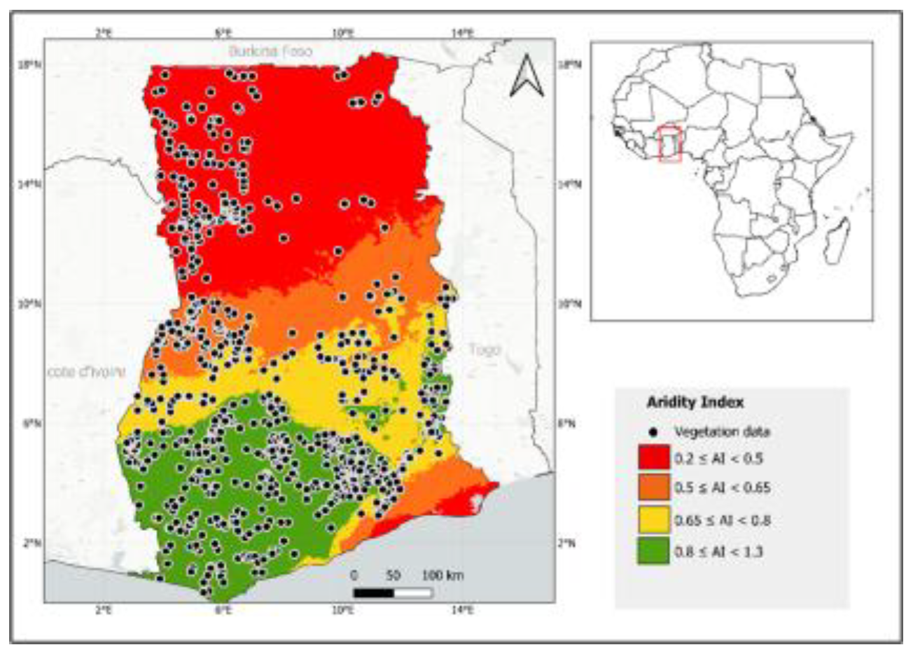
Figure 2.
Boxplot showing the distribution of above-ground biomass (AGB) across four aridity classes (Humid, Sub-humid, Dry sub-humid, and Semi-arid). Diamonds show group means. Letters above boxes are from Scheffé post hoc test (a = 0.05): groups sharing the same letter are not significantly different, while different letters indicate significant differences. Aridity classes follow the UNEP AI classification.
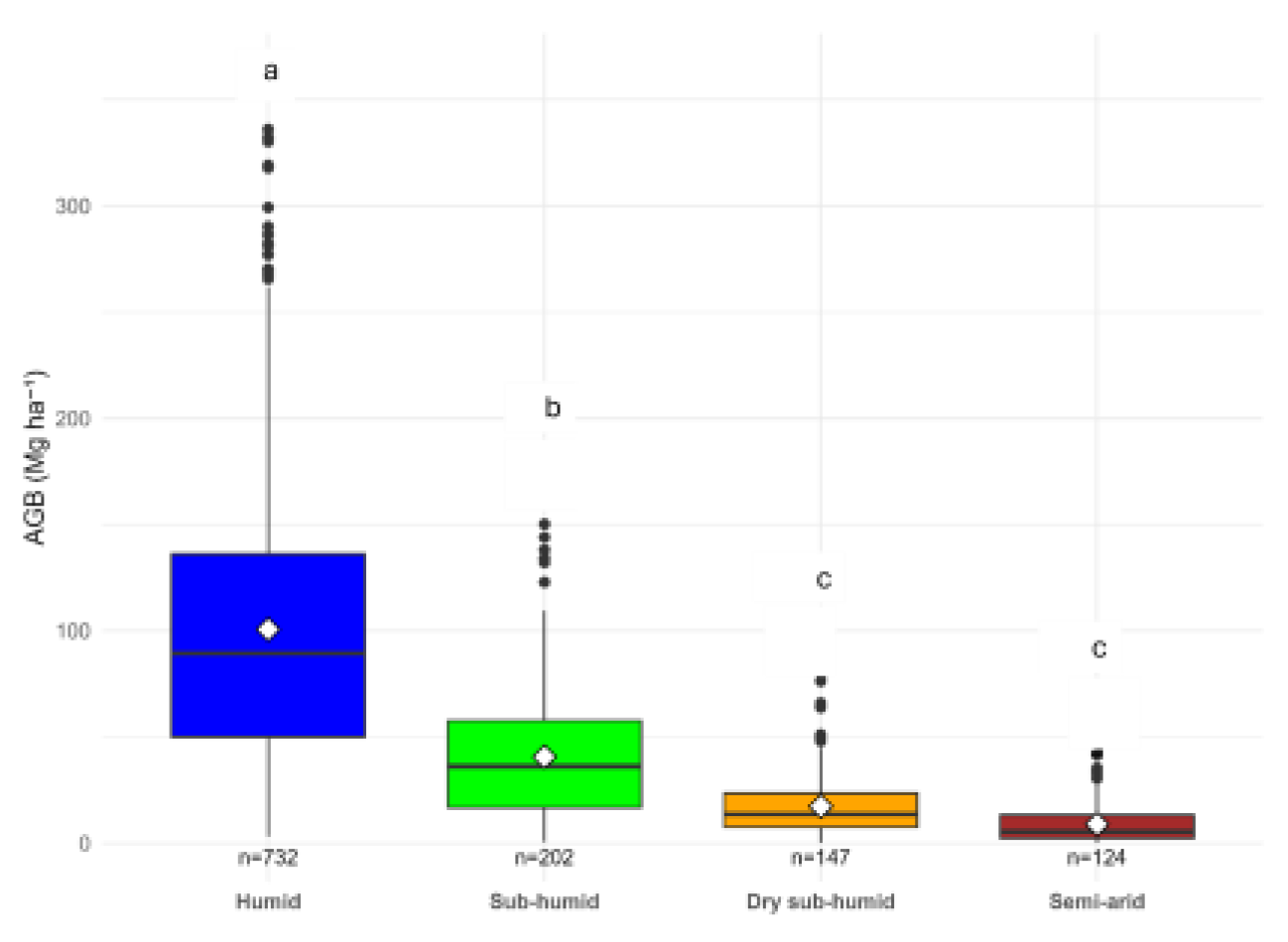
Figure 3.
Structural equation models illustrating the direct and indirect effects of aridity index (AI) on above-ground biomass (AGB_cal) through forest fragmentation (PCA composite: Frag_PC1) and biodiversity (species richness). (a) Linear SEM (GLS-based) showing standardized path coefficients (β) and significance (p-values). Green arrows indicate positive relationships, and orange indicate negative relationships. Solid lines denote significant paths, dashed green arrows represent non-significant but positive relationships. (b) Nonlinear SEM (GAM-based) showing smoothed functional relationships among AI, Frag_PC1, species richness, and AGB_cal. Arrow color indicates the direction and significance of effects: green = positive and significant, orange = negative and significant, and gray dashed arrows = non-significant paths.
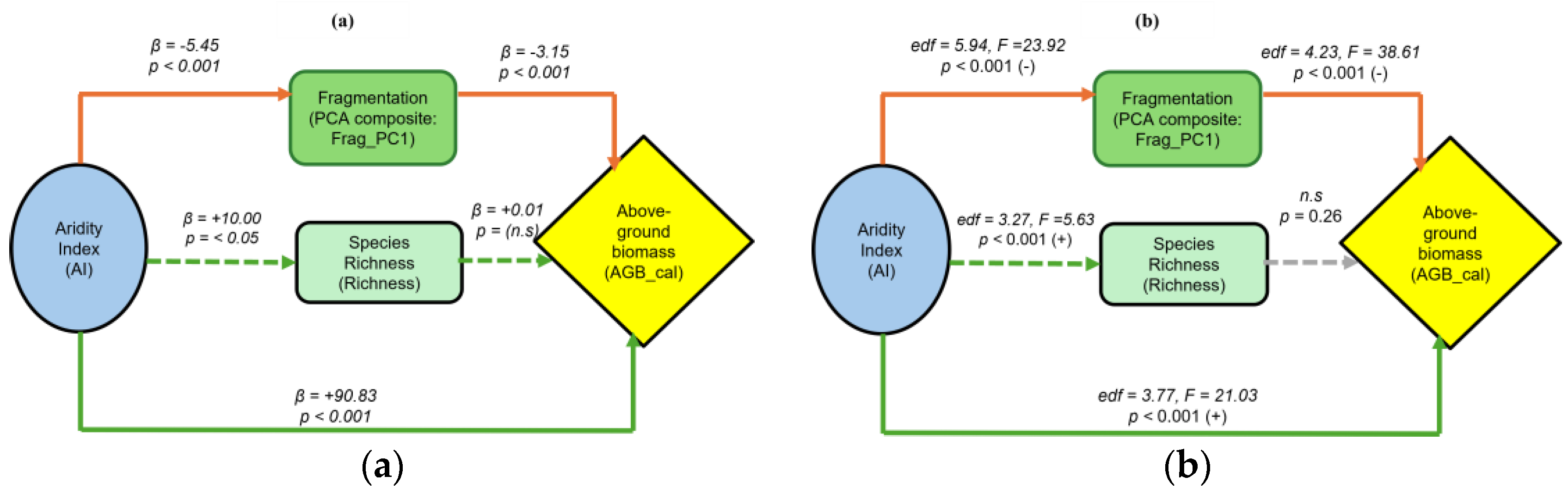
Figure 4.
Partial effects for individual fragmentation metrics (NP, AREA_MN, ED, MSI, LSI).
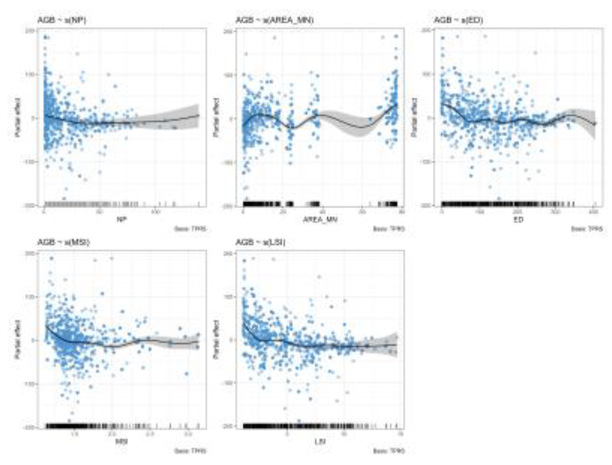
Table 1.
Classification of Ghana’s climate zones based on the Aridity Index (AI) and their land area coverage. The aridity (AI) thresholds follow the UNEP aridity classification scheme.
Table 1.
Classification of Ghana’s climate zones based on the Aridity Index (AI) and their land area coverage. The aridity (AI) thresholds follow the UNEP aridity classification scheme.
| Aridity index (AI) values | Climate class (zones) |
|---|---|
| 0.2 ≤ AI < 0.35 | Semi-arid |
| 0.35 ≤ AI < 0.5 | Dry sub-humid |
| 0.5 ≤ AI < 0.65 | Sub-humid |
| AI ≥ 0.65 | Humid |
Table 3.
Mean above-ground biomass (calibrated AGB) by aridity class.
| Aridity class | Sample size (n) | Mean AGB (Mg ha-1) | SD (Mg ha-1) | Scheffé group |
|---|---|---|---|---|
| Humid | 732 | 217.34 | 152.82 | a |
| Sub-humid | 202 | 70.13 | 69.61 | b |
| Dry sub-humid | 147 | 18.71 | 26.44 | c |
| Semi-arid | 124 | 7.30 | 13.83 | c |
Letters indicate Scheffé-adjusted significance groups (a = 0.05); classes sharing the same letter are not significantly different.
Table 4.
Model-fit statistics and variance (R2) for linear and nonlinear structural equation models linking aridity (AI), fragmentation (Frag_PC1), biodiversity, and AGBB, AIC = Akaike Information Criterion; Fisher’s C = global test of model fit; df = degree of freedom; R2 values represent variance for each endogenous variable.
| Model type | AIC | Fisher’s C | df | p-value | R2(AGB_cal) | R2(Frag_PC1) | R2(Richness) |
|---|---|---|---|---|---|---|---|
| Linear SEM | 4178.46 | 3.04 | 2 | 0.219 | 0.620 | 0.304 | 0.004 |
| Nonlinear SEM | 8130.84 | 226.34 | 18 | < 0.001 | 0.834 | 0.154 | 0.032 |
Table 5.
Spatial GAM smooth terms for AGB with each fragmentation metric modeled separately, while controlling for s(AI) and s (x, y), ∆AIC and ∆Dev are relative to baseline model AGB ~ s(AI) + s (x, y). Not applicable () for AI and biodiversity terms. Rows marked with * are taken from the main AGB model used for Figure 4.
| Predictor | edf | F | P | ∆AIC | ∆Dev |
|---|---|---|---|---|---|
| AI* | 3.71 | 13.74 | <0.001 | ‒ | ‒ |
| NP | 2.68 | 4.91 | <0.001 | 71.21 | 0.009 |
| AREA_MN | 6.95 | 46.70 | <0.001 | 386.25 | 0.043 |
| ED | 7.09 | 31.59 | <0.001 | 268.51 | 0.031 |
| MSI | 5.65 | 15.14 | <0.001 | 156.77 | 0.020 |
| LSI | 6.60 | 29.73 | <0.001 | 256.44 | 0.030 |
| Richness* | 0.60 | 0.39 | 0.052 | ‒ | ‒ |
Disclaimer/Publisher’s Note: The statements, opinions and data contained in all publications are solely those of the individual author(s) and contributor(s) and not of MDPI and/or the editor(s). MDPI and/or the editor(s) disclaim responsibility for any injury to people or property resulting from any ideas, methods, instructions or products referred to in the content. |
© 2025 by the authors. Licensee MDPI, Basel, Switzerland. This article is an open access article distributed under the terms and conditions of the Creative Commons Attribution (CC BY) license (http://creativecommons.org/licenses/by/4.0/).
Copyright: This open access article is published under a Creative Commons CC BY 4.0 license, which permit the free download, distribution, and reuse, provided that the author and preprint are cited in any reuse.


