
Submitted:
11 June 2025
Posted:
13 June 2025
You are already at the latest version
Abstract
Anthropogenic and climatic pressures can transform contiguous forests into smaller, less connected fragments. Forest biodiversity and ecosystem functioning can further-more be compromised or enhanced. We present a descriptive analysis of recent forest fragmentation in Bavaria, the largest federal state in Germany. We calculated 22 metrics of fragmentation on forest polygons, aggregated within administrative units and with respect to both elevation and aspect orientation. Using a forest mask from September 2024, we found 2.384 million hectares of forest across Bavaria distributed amongst 83,253 forest polygons 0.1 hectare and larger. XS patches (< 25 ha), outnumber all other size classes (25-160 ha, 160-789 ha, 789-3,594 ha, and 3,594-48,703 ha) by nearly 13 to 1. Edge zones, where microclimatic effects may distinguish an area up to 100m from the forest perimeter, accounted for more than 1.68 million hectares, leaving less than 703,000 remaining hectares as core forest. Although south-facing slopes dominated the state, the highest forest cover (~36%) was found on least abundant east-oriented slopes. Most of the area is located at 400-600 m.a.s.l. with around 30% of this area covered by forests, however, XL forest patches (> 3,594 ha) dominated higher elevations, covering 30-60% of land surface area between 600-1400 m.a.s.l. The distribution of the largest patches follows the higher terrain and corresponds well to protected areas.
Keywords:
remote sensing
; disturbance
; forest loss
; Germany
; landscape ecology
; temperate forest
; bark beetle
; central Europe
; forest management
1. Introduction
The threat of temperate forest degradation due to the effects of climate change is steadily escalating [1,2,3]. Forests provide numerous indispensable ecosystem services, especially the reduction and storage of atmospheric carbon [4,5], cooling of the land surface [6,7] and regulation of the hydrosphere [8,9]. Consequently, the loss of trees, and therefore vital forest structure, compromises the climate buffering function of forests (Mann et al., 2023). Reduced forest area together with an increase in the number of isolated forest patches can furthermore have consequences for forest species and ecosystem functioning as interactions between them may change unpredictably. Thus, analyzing spatial patterns of forests is essential for understanding their role in maintaining biodiversity, supporting ecosystem functions, and enhancing climate resilience.
1.1. Fragmentation Versus Forest Loss
Fragmentation refers to the discontinuous pattern of forest patches within a landscape. Such patterns can arise from human activities (logging, historical land use or land use conversion, construction of infrastructure, soil pollution), from natural causes (windthrow, insect infestations, drought, floods, wildfire), the underlying properties of the substrate (soil type & texture, hydrology, persistence of rock outcrops) or other biophysical constraints (temperature, elevation/terrain, precipitation, solar irradiance) which contribute to the natural patchiness of landscapes. The combination of these drivers results in a landscape mosaic, which is characterized by a spatially uneven distribution of landcover types, comprised of for example forests, agriculture, water bodies, and infrastructure. Except for the most remote forests, anthropologically developed regions exhibit patchy forest patterns. In other words, landscape patchiness is the rule, not the exception [11,12].
Fragmentation occurs when forests are broken apart into more numerous and disconnected patches, and can be considered as a distinct process from habitat loss [13,14]. With fragmentation per se, patches can become disconnected but the same amount of habitat area within a given landscape can still be maintained. Habitat loss, on the other hand, is a process whereby the area of forest is reduced over time. Figure 1 illustrates this concept using four scenarios of habitat loss. In the first frame, the forest covers 100% of the landscape, in the next the forest is reduced to 50%. Finally, the forest is reduced to 25% of the original size in the last frame. In the shrinkage scenario, forest habitat is lost, but not fragmented. This is also true in the perforation scenario, because forest connectivity is maintained even as the forested area is reduced.
Bisection and fragmentation are characterized by the dis-connectivity of forest area, which we refer to as fragmentation. The figure illustrates both forest loss and fragmentation of remaining habitat but it is important to distinguish this phenomenon from landscapes where the overall forest area is maintained across an increased number of individual patches. This scenario is typically referred to as ‘fragmentation per se’ as opposed to merely fragmentation [15]. Figure 2 exemplifies the fragmentation of forest without a reduction in overall forest area within the landscape. This distinction is significant, because the maintenance of habitat area within a specified landscape despite fragmentation, can still support animal habitats and ecosystem functioning [13].
Because of the heterogeneity of landscapes, the degree of fragmentation of forests within them is variable. To understand the relative intensity of fragmentation, it is useful to assess landscape patterns in terms of forested area and number of fragments, or the ‘patchiness’ of forests, within the landscape. Table 1 summarizes the degree or intensity of expected fragmentation based on these factors, resulting in different levels of forest fragmentation.
1.2. Aggregation and Isolation
Although disconnected patches may have altered functional capacity in terms of ecosystem services, biodiversity, habitats and resilience against the effects of climate change [17,18,19], counterintuitively, fragmentation can favor some species whilst disadvantaging others. This depends on the scale, distribution (isolation or aggregation of patches), cause, frequency and degree of forest loss (if any) and the affected species. This paradox has been investigated in a wide range of habitat types, climate zones and under various drivers of habitat loss [16]. In the majority of cases, Fahrig et al. determined a net positive effect of fragmentation independent of habitat loss.
Furthermore, while larger forests reliably support more species, disconnected habitats can genetically isolate populations thereby contributing to speciation over long time scales. However, the lack of incoming genetic diversity can also lead to population decline. Moreover, reduction in habitat area predictably reduces species richness within patches. These principles were the foundation of the theory of island biogeography [20].
Although initially developed for oceanic islands, this theory came to dominate the conceptual understanding of early investigations of fragmented terrestrial habitats. However, it is important to note that islands in an ocean are not directly analogous to terrestrial habitat patches. Forests are embedded in a mosaic of other landcover types that have distinctive properties which can facilitate or hinder animal movement and plant dispersion. To simplify this concept, we focus on the number of neighboring forests to each forest and their distance to understand the isolation or aggregation of forest patches within a landscape. Table 2 summarizes these concepts below.
The degree or intensity of patch isolation can thus limit or enhance the quality and quantity of species interactions. Species interactions drive underlying processes such as forest seed dispersal by birds or rodents, the movement of pathogens or infectious diseases, facilitation of gene flow or reproduction. These processes require the interaction of species within available habitat which is further modulated by habitat configuration and distribution. Fragmentation of forests therefore has species-specific effects.
1.3. Edge Structure
In unmanaged forests, where human inventions are minimal or absent, forest is lost by the aforementioned natural causes which occur at less frequent intervals than anthropogenic drivers, but can nevertheless cover large spatial areas. However, remaining forest structure (vertical layers, lying deadwood) and perimeter morphology (straight versus sinuous) are typically more heterogenous compared to human-caused forest loss [11,12,21]. The resulting structural differences between natural and anthropogenic fragmentation can favor some forest species while harming others. This is especially true for the region where interior forest is lost (perforated) where, like forest edges, microclimatic conditions differ from the interior of a forest. These abiotic conditions can furthermore be modulated by the remaining forest structure, perimeter morphology, and the adjacent landcover type [21]. This may increase biodiversity by favoring generalist species which can easily colonize disturbed areas and prefer higher light, temperature and windy conditions [22].
Forest structure can vary by species, management practices, age class, and distance to the forest perimeter [23]. For example, trees along a mature perimeter, where the vegetation has developed according to the edge conditions, often exhibit branches at lower positions on stems. Whereas a newly exposed (disturbed) perimeter, where trees had developed with greater light competition within the forest interior, branches tend to dominate higher positions. Thus, stems become exposed to abrupt changes in abiotic conditions. This difference in structure modulates a profound ‘edge-effect’ which is caused by the penetration of sunlight, thereby creating microclimatic conditions along perimeters and in edge zones [24]. Although disturbances are usually transient, the effect on growth of surrounding trees can persist even after perforations or edges have regrown [25]. Figure 3 characterizes the variability along a mature perimeter (A) and a recently disturbed perimeter (B, C) of spruce-dominated forest near Garmish-Partenkirchen (A, B) and Wessling (C).
To conceptualize the amount of edge in a forest or landscape, it is necessary to also account for the area of forests. If the overall amount of forest is large, the area where edge effects occur is relatively small. By the same token, in landscapes or patches with a small forested area, perimeters and thus edge effects, will tend to dominate the forest. This is significant, because trees stressed by temperature may be less resilient to droughts, insect infestations, or other disturbances [26]. Table 2 summarizes the so-called edginess potential for different ratios of forest area to perimeter length.

Table 2.
The ‘edginess’ or amount of edge is a function of the length of the perimeter of forest patches and the area of patches within the landscape.
Table 2.
The ‘edginess’ or amount of edge is a function of the length of the perimeter of forest patches and the area of patches within the landscape.
| Perimeter length | Patch area | Interpretation | Edginess |
| High | Low | Patches are likely long and narrow with very little if any core area | High |
| High | High | Patches are large and may have numerous perforations, edge effects are likely minimal | Low to moderate |
| Low | Low | Patches are likely small, geometric, perhaps without any core area | Moderate to high |
| Low | High | Patches may be medium sized with few or small perforations | Low |
Geospatial forest fragmentation analysis focuses on three essential zones of the forest; the perimeter, edge zone, and the core of individual patches. The edge zone is a transitional region of forest up to 100m interior to a forest perimeter which can act as a microclimatic buffer for the core zone, which is the remaining interior region [27]. Depending on management practices, perimeters and edge zones usually exhibit different biotic and abiotic characteristics and conditions compared to forest interiors in addition to increased occurrence of invasive species (Figure 4, A-E) [28].
1.4. Fragmentation Analysis
Importantly, fragmentation must be analyzed within the context of a defined landscape area [30]. Characteristics of forest patches such as amount & distribution, perimeter length, core and edge area, shape, and neighboring patch configurations can then be aggregated within landscape boundaries. Landscapes can thus be utilized as units for ecological investigations, for example investigations regarding forest species abundance based on total habitat amount within or amongst discontinuous patches. To determine the intensity of fragmentation, the number of fragments, patch distribution, and edginess can then be related to the remaining metrics within a landscape unit.
Analysis of remotely sensed imagery is an effective approach for monitoring forest condition and disturbance [31], is an under-utilized tool in the study of forest fragmentation, and is furthermore ideal for large-scale applications [32]. Given the profound differences between fragmented forests and contiguous forest ecosystems [33], an assessment of fragmentation in the largest and most forested state in Germany is needed. Furthermore, the topic has not yet been investigated on the state-scale using Earth observation (EO) data [34]. Understanding landscape patterns and processes is moreover important for the formulation and assessment of forest management strategies within the context of climate change and conservation. Therefore, fragmentation across Bavaria can be efficiently investigated by analyzing satellite data and is the subject of this inquiry. We present:
- A characterization of forests using structural and functional fragmentation metrics based on patch size categorization
- The spatial and terrain distribution of fragmentation
- State-, county-, and district-level results which can support data-driven forest policy and management decisions
2. Materials and Methods
2.1. Study Area
Forests characterize more than one-third of the land surface in Bavaria and are comprised of predominantly Norway spruce (Picea abies), European beech (Fagus sylvatica), Scots pine (Pinus sylvestris), and oak (Quercus sp.), with larch (Larix sp.), fir (Abies sp.), maple (Acer sp.), birch (Betula sp.) and others making up smaller fractions. The species composition varies based forest ownership and management, patch size, protection status, and elevation [35]. Broadly speaking, species distribution follows a gradient whereby broadleaf deciduous forests dominate Lower and Middle Franconia, and coniferous species, namely spruce dominate in higher elevations of the remaining districts becoming monocultures along the eastern and southern borders of Bavaria [36]. Mixed forests are typically found at elevations less than 600 m.a.s.l. and can be the result of careful forest management practices. In recent years, there has been a push to increase the diversity of mixed forests due to the apparent resiliency of mixed over mono-cultured forests [37].
Bavaria exhibits a heterogenous mosaic of landcover types. Forests, urban areas, rivers, agriculture and transportation infrastructure form a patchy landscape across the state; a consequence of historical land use practices, soil types, and topography. Large charismatic animal species including lynx (Lynx lynx), roe and red deer (Capreolus capreolus, Cevus elaphus), capercaillie (Tetrao urogallus), hazel and black grouse (Tetrastes bonasia, Lyrurus tetrix), moose (Alces alces) and even wolf (Canis lupus) can be found especially within the protected forests, like the Bavarian Forest National Park (BFNP) [38]. Moreover, landscapes and patches across Bavaria provide key habitats, including the last colony of greater horseshoe bats (Rhinolophus ferrumequinum) in Germany [39], and for migrating birds such as Eurasian cranes (Grus grus) and white storks (Ciconia Ciconia) [40,41].
The state of Bavarian forests today is a result of historical development and recent management schemes. Germany was subject to post-war reparations which were partly paid in the form of timber. This left the region in need of efficient afforestation strategies, which resulted in vast deliberate replanting of non-native Norway spruce [42]. This fast-growing conifer quickly reforested areas of Germany that were less vital for agriculture and infrastructure, particularly higher elevations, steep slopes, and in less productive soils. The spruce still forms the foundation of the forestry sector. However, the natural forest condition of Germany, which developed after the last glacial period, was broadleaved deciduous species. Initially oak and later beech dominated the landscape; the European beech is still the most common deciduous tree in Bavaria.
Large regions of state-owned forest in Bavaria are under a protected status. Nature reserves & parks, biosphere reserves, Natura2000 sites, and national parks together cover about one-third of the forest area [43,44]. In Figure 5, national parks are depicted separately from all other levels of protection (Figure 5 A). However, most of the forested area in Bavaria is privately owned (Figure 5 C). Topography in Bavaria varies from low mountain ranges in the north and middle of the state, to pre-alps in the south reaching nearly 3000 m.a.s.l. (Zugspitze, 2962 m). Most of the land area is less than 600 m.a.s.l. (Figure 5 B). The climate follows a similar spatial gradient whereby northern counties are warmer and drier, and southernmost districts within Swabia and Upper Bavaria, and Lower Bavaria in the east, are cooler and wetter. In recent decades, climate across the state has shifted to more mild winters and hotter, drier summers (Figure 5 D, E).
2.2. Data
The workflow for the methodology is presented in Figure 6. All data processing and preparation of figures was completed in Jupyter Lab [45] (version 4.0.6) using Python [46] (version 3.10.12). Maps were produced using the matplotlib package [47] and using QGIS [48] (version 3.34.13).
The resolution and update frequency of commonly used Copernicus forest cover products varies by product [49,50,51]. Therefore we have instead applied the most recent release of the (1) the Germany-wide forest mask developed by Thonfeld et al. [52] (updated until September 2024) and (2) the digital elevation model (DEM) produced by the Bavarian Surveying Authority [53] in this analysis (Table 4). Both datasets were re-projected using the rasterio package [54]. The EPSG: 3035 projection was selected due to area preservation, in order make the most accurate geometric calculations for fragmentation analysis. Both datasets were then masked to the study area (the federal state of Bavaria) using an administrative shapefile of the same projection.
2.3. Methodology
Fragmentation analysis is a method for understanding spatial patterns among patches of a particular habitat within a defined landscape [30]. Here we delineated the small-scale patterns among forest patches, referred to as patch-scale. Large-scale patterns are also referred to as landscape-scale patterns where a given landscape is defined. We focused on the administrative unit as the landscape based on forest management practices, rather than on the basis of an ecological landscape scale. The purpose of this definition is to support policy and forest management decisions which are often defined at the scale of administrative rather than ecological units.
FCCL Forest Mask raster data were vectorized to delineate discreet forest polygons larger than 0.1 ha. Forest polygons were then masked by county and district-level administrative boundaries in the EPSG: 3035 projection. Metrics of forest fragmentation were selected based on FRAGSTATS definitions [55,56]. We then developed an independent calculation processing chain in Python to derive fragmentation metrics. Metrics were divided into two categories: structural (size, shape, amount) and functional (spatial distribution) characteristics (detailed in Table 2). Within these two broad categories, 14 metrics of fragmentation were compiled using the processing chain. Furthermore, these metrics were aggregated by sum, mean, or both, resulting in 22 total measurements (Table 5).
We integrated terrain data into our characterization for a comprehensive spatial overview of the status and distribution of forest fragmentation in Bavaria. The 1m digital elevation model (DEM) produced by the Bavarian Surveying Authority was resampled to 10 m and re-projected (matching all data sources). The aspect was derived from the DEM using the rasterio [54] and numpy [57] libraries. Using the equal interval method, we binned the DEM data into 200m elevational zones beginning at zero and using 3000 meters above sea level (m.a.s.l.) as the maximum elevation. True elevations across Bavaria range from 108 to 2962 m.a.s.l. To derive the percent forest cover for each elevation zone, we used the overlay function to intersect the forest mask data with the elevation data, using the forest patch size categorization as subsets.
Similarly, we categorized the aspect data into four orientation bins using 315° – 45° as North, 45° - 135° as East, 135° - 225° as South, and 225° - 315° as West. The resulting multipolygons for each aspect orientation were dissolved into a single layer and intersected using the overlay function with the forest mask data, subset by forest patch size category.
Following FRAGSTATS definitions, we distinguished metrics by landscape pattern into two categories; structural and functional. Structural elements measure spatial or geometric attributes of forest (or other habitat) patches within a selected landscape unit. In the present study, the administrative unit is the landscape. Functional metrics consider the distribution of patches within a landscape with respect to surrounding nearby patches. When considered in the context of other metrics, structural and functional elements can uncover patterns and intensity of forest fragmentation.
2.3.1. Area
Metrics are presented with increasing complexity, starting with area, which considers individual patches and their aggregated area within a landscape or administrative unit. This and subsequent area measurements are given in hectares. The area of forest within a landscape distributed amongst the number of patches can suggest the intensity of fragmentation (see Table 1.).
2.3.2. Core Area
The category of core area considers a defined edge depth where the effects of sunlight, temperature, wind, and soil moisture differ from the interior of the forest. This depth can depend on several factors including climate, topography, canopy cover, species composition, and disturbances ranging from harvesting operations to insect infestations. In this study, following the literature [58] we have characterized core area with a 100m edge depth.
2.3.3. Edge Area
Edge area can be conceptualized as the inverse of the core area. Edges are divided into two metrics, the perimeter length (given in meters), and the area of the edge zone which is derived using the aforementioned edge depth employed in the core area calculations and expressed as the sum, mean, and percent. The amount of perimeter or edge area relative to the total area or core area of forests within a landscape can be used to understand the dominance of edge effects in a landscape or single forest (see Table 3.).
2.3.4. Perforations
Perforations are gaps that form as a result of disturbances in the core area of a forest. They can be measured in terms of their overall distribution by both amount and area, and the percent of the forest in which they are located. The result of perforations is effectively an increase in the perimeter and thus the edge area of the forest.
2.3.5. Shape
Two metrics for measuring shape were selected for this analysis. The perimeter-area ratio and the shape index. Taken together, shape metrics can reveal complexities in forest patch geometry that arise from forest canopy loss. Complex shapes equate to longer perimeter lengths (including within perforations) resulting in increased edge area where trees are exposed to abiotic elements.
2.3.6. Neighborhood
Neighborhood metrics are calculated by constructing a buffer (radius 200m in this analysis) around each forest patch. The patch edge-to-edge distance is measured within the buffer area. Metrics calculated include the number of neighbors within the 200m buffer, the distance between them, and in addition, the area of these neighboring patches. The aggregation or isolation of individual patches and forested landscapes can be inferred from the number of neighbors and the average distance between patches within a landscape (see Table 2.)
2.4. Metric Aggregation
Metrics were analyzed at the forest patch level and aggregated at the landscape level. Administrative units (state: Land, county: Regierungsbezirk, district: Landkreis) were used to delineate landscape borders. Where forest patches straddled an administrative border, the patch was divided (clipped) by the administrative polygon and the metrics were calculated and aggregated only for the area within the administrative unit. This scenario is not common and therefore did not result in meaningful increases in patch number.
3. Results
We delineated 83,253 individual forest polygons (hereafter patches) which contained roughly 2.384 million hectares of forest in Bavaria. Patches ranged in size from 0.1 (based on the minimum forest size, defined by the German Federal Ministry of Agriculture, Food and Regional Identity, BMEL [59]) to ~ 48,703 hectares, however the distribution of patch sizes is not normal. Figure 7 visualizes the distribution of patch sizes after applying a log-transformation of the data. Due to the skewed nature of these data, we present the fragmentation characterization in categories based on forest patch size.
Size categorization or binning was performed on the state-wide dataset using the Jenks-Caspall method [60] for clustering geospatial data. JenksCaspall optimizes bins to minimize variance within and maximize differences between bins, and is therefore well-suited for skewed data. The operation was conducted using the mapclassify library in Jupyter Lab (version 4.0.6) using Python (version 3.10.12), resulting in 5 size bins. The smallest size bin, 0.1-25 hectares is hereafter referred to as the XS size class. In order of increasing forest size, patch categorization is as follows: 25-160 hectares (S), 160-789 hectares (M), 785-3,594 hectares (L), and 3,594-48,703 hectares (XL).
The spatial distribution of patch sizes across the state of Bavaria is heterogenous. The largest forest polygons are located around the periphery of the state, namely in the northwest corner of Lower Franconia, the central and eastern regions of Upper Franconia, Upper Palatinate, and Lower Bavaria, and the southern regions of both Swabia and Upper Bavaria. The distribution roughly follows both the terrain of the state, with the largest contiguous forest polygons located at higher elevations, as well as the areas with a status of varying degrees of forest protection as nature areas, reserves, or parks at both the state and federal levels. Figure 8 (A) presents an overview of the spatial and size category distribution with inset examples of fragmentation patterns.
Figure 8 (B and C) summarize the distribution of patches with regards to terrain. In Figure 8 (B), above 2000m there is no forest cover and was therefore omitted from this figure. The total area of each elevational zone is represented on the right y-axis with bars outlined in black (1x10⁶ ha). The 1000-1200m elevational zone contains the highest percent of forest cover at just over 60% however this zone is among the smallest, covering about 120,000 ha. The lowest elevational zone, 0-200m, is covered by less forest than each subsequent zone until the climatic conditions limit tree growth above 1400m. The smallest forest patches are relatively evenly distributed across the elevational zones compared to L and XL patches which make up the largest share of forest coverage as elevation increases. Most of the land surface area of the state falls within the 400-600m elevation zone (about 3.75 million ha), however only about 30% is covered by forested area.
The total area is not evenly distributed amongst the four aspect directions (Figure 8 C). The majority of slopes are south-facing and have the second highest percent forest cover. The smallest slope category was East; however, these slopes have the highest percent coverage of forest. West-facing slopes had the smallest coverage overall.
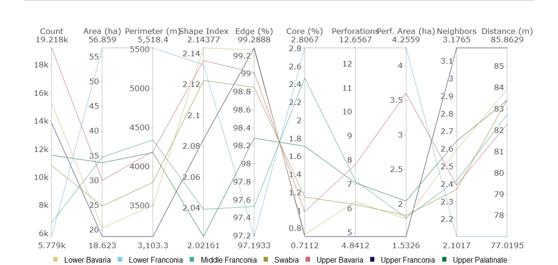
Figure 9 visualizes the state-wide results of forest fragmentation pattern characterization covering the whole of Bavaria using min-max scaling. Results are organized by the abovementioned patch size bin categorization. For detailed results tables for the state and each county of Bavaria, we refer the reader to the Supplementary Materials.
3.1. Area and Number of Patches
Most forests (77,175 patches) were categorized as XS (< 25 ha), however this category covered the smallest area overall. More than 92% of forest patches cover an area less than 25 ha each, with a total area of 192,177 ha or about 8% of the total forested area in the state. The mean area of XS patches was 2.5 ha and this varies by district. The largest patches (XL), those at least 3,594 ha cover a total of 976,504 ha amongst 101 patches, which is 41% of forested area in Bavaria. Upper Bavaria had both the largest area of XL patches (296,475 ha) distributed amongst 21 forest polygons, and the highest number of XS forest patches (17,847).
3.2. Core and Edge Area
A 100m edge depth was considered in this analysis. The remaining interior forest area not contained within the edge zone is considered core forest. Among the XS fragments, 99.8% lies within the 100m edge zone. The resulting mean core areas in these patches is 0.2 ha. Edge and core area increased with increasing patch size category. However only among patches L or larger is the average core area higher than 30%. This suggests the patch shape is highly irregular, with longer perimeter lengths and more perforations with respect to forest patch areas. For the largest fragments (XL), the average core area is 38%.
3.3. Perimeter
Total perimeter length did not have a strictly positive or negative correlation with patch size category. Instead, both the XS patch and XL patch categories had the longest total perimeter lengths; about 83.9 and 84.6 million meters respectively. Whereas the S, M, and L patch size categories had total perimeter lengths of ~51.5, ~52, and ~57 million meters respectively. Due to the total length of perimeter and small individual patch areas, the perimeter-area ratio, or ‘paratio’, was highest among fragments in the XS category.
3.4. Shape
Patch shape was measured using two metrics; the ‘paratio’ and the shape index. Paratio decreased with increasing patch size, which reflects the larger patch area with respect to patch perimeter length. Shape index increased with patch size which suggests an increase in shape complexity, meaning shapes diverge from simple geometric forms (circles, squares). Shape complexity also increases with the occurrence of perforations (see 3.5.). In Figure 10, we present examples of increasing shape complexity (A-H).
3.5. Perforations
The number and total area of forest perforations or gaps increased with patch size and varied widely between counties. Less than one gap existed per XS patch on average meanwhile the largest fragments contained on average more than 2,300 gaps across the state. Upper Bavaria had the largest area of perforations (69,164 ha), while Middle Franconia had the smallest area (12,237 ha).
3.6. Neighborhood
With respect to functional fragmentation, the patterns were not necessarily linearly correlated to patch size. Instead, XS forests had the highest total number of neighboring patches within a 200m buffer area, followed by S, M, XL, and L fragments. However, the average number of neighbors increases based on patch size category. XS patches on average have 2.1 neighbors which increased with each successive larger patch. XL patches had an average of 99 neighbors each. Although the mean area of neighboring forest polygons varied by patch size, neighboring forest patches to XL fragments were on average the largest compared to other patch sizes.
The distance between neighboring patches also varied between patches sizes and counties. In general, the distance between patches increased depending on the size of the patch. The nearest or most aggregated patches were among the XL patches and surrounding neighboring patches in Lower Franconia which were on average 58.3 meters apart (considering patches within the 200m buffer), while the longest distance between neighbors on average was 86.3 meters amongst the XS patches in Upper Franconia.
3.7. Spatial Distribution
Figure 11 and Figure 12 visualize the spatial distribution of fragmentation density patterns, aggregated at the district level in Bavaria. The metrics have been normalized by district area in order to make meaningful comparisons, and the sparse data within municipalities has been masked (grey polygons) to remove noise from the district dataset.
3.7.1. Patch Count Density
Kronach district in the northeastern region of Bavaria has the highest density of forest fragments (total number of fragments normalized by district area), followed by neighboring Kulmbach and Hof districts, and Passau district in the east. Figure 11 (A, a) highlights the high number of fragments in Passau district. Districts with lower patch densities were more evenly distributed across the state, with the county surrounding the city of Munich in the southern district of Upper Bavaria having the lowest density of patches per district area.
3.7.2. Area Density
Districts with the largest total forest area with respect to district area include Main-Spessart (inset, Figure 11 B, b), Aschaffenburg and Miltenberg in Lower Franconia; Regen and Freyung-Grafenau (corresponding to the Bavarian Forest National Park - BFNP) in the east, and Miesbach, Bad Tolz-Wolfratshausen, and Garmisch-Partenkirchen districts in southern Upper Bavaria.
3.7.3. Core Area Density
The ratio of core forest with respect to the total area per district follows similar trends as the total forested area. Districts surrounding the city of Munich have the least core forest including Dachau, Freising, Erding, Landshut, and Mühldorf. Kronach district is shown in the inset map (Figure 11 C, c) with low core forest area density.
3.7.4. Perimeter Density
Density of forest perimeter lengths tended to be higher in the north, east, and south of Bavaria. This was especially the case in Kronach and surrounding districts in Upper Franconia and the area surrounding the BFNP in the east. Oberallgau district is shown in the inset map (Figure 11 D, d).
3.7.5. Shape Complexity Density
Figure 12 (A) presents the distribution of the mean shape complexity index. As the index increases, forest patch shape deviates from simple geometry becoming increasingly complex especially for patches with long perimeter lengths and perforations. Patch shape complexity is distributed relatively evenly across the state with some exceptions of low mean complexity including Cham and the districts surrounding Nuremburg (Forchheim, Erlangen-Höchstadt, and Fürth). The inset map (Figure 12 a) presents the index in Altötting district where long narrow forest patches with perforations are common.
3.7.6. Perforation Density
Forest perforations (Figure 12 B) are particularly abundant in districts Kronach, Regen, Freyung-Grafenau, Traunstein (inset map, Figure 12 b), and Berchtesgadener Land which are also heavily forested districts, whereas districts with the smallest patch sizes also had the fewest number of forest gaps (those situated outside of Munich and Nuremberg). The highest density of perforations was found in the southern districts of Miesbach and Garmisch-Partenkirchen (inset map, Figure 12 c); as well as in Berchtesgadener Land, Regen, and Freyung-Grafenau in the east. Eichstatt in the center of Bavaria north of Ingolstadt has a notable density of perforations, unlike the surrounding districts.
3.7.7. Perforated Area Density
The highest density of perforated area was found in Miesbach district followed by Garmish-Partenkirchen (Figure 12 C and inset, c) and Regen districts. Berchtesgadener Land, Freyung-Grafenau, Bad Tölz-Wolfratshausen, Eichstätt, Forcheim, and Miltenberg districts also had high densities of perforated area. Districts with the least perforated area density were also districts with the smallest overall density of forest area, namely those east of Munich in Upper and Lower Bavaria.
3.7.8. Neighborhood density
The number of neighboring patches found within a 200m buffer of every forest fragment was highest in Kronach district, a region with high total forest area and a high density of patches relative to the area of the district. In Donau-Ries district, forest patches have few neighboring patches, meaning forest patches are more isolated (Figure 12 D, d).
4. Discussion
4.1. Number of Forests, Core Area, and General Distribution
Large forests represent roughly one-third of the total forested area of the state. The largest forests are located primarily in remote mountainous regions of the state, above 600 m.a.s.l., are typically state-owned, dominated by spruce and classified as parks or reserves.
The value of ecosystem services provided by large forests, including regulation of the hydrosphere, cannot be replaced by any other means [8]. Therefore, the protection and management of large forests is vital [61]. Large, continuous core areas are especially important for carbon reduction & storage, and land surface temperature regulation (Mann et al., 2023). In Bavaria, XL forest patches together contain over 180 times the core forest area of the XS patches combined. However, due to drought and bark beetle disturbances to spruce, recent large-scale forest loss has caused a major shift. Since 2017, the forests of Germany are now a source of carbon rather than a sink [59]. How long this trend continues is a question of forest management particularly in terms of nature conservation and tree species composition.
Among the smallest patches, the ratio of edge to core is such that only a small percent of forest can provide valuable core-specific habitats and ecosystem services. Meanwhile edge effects dominate small forests and stress edge zone buffer trees, which can lead to further forest loss. Regardless, small forest patches can still deliver ecosystem services, provide habitats, and habitat connectivity across a landscape, and should therefore not be discounted as valueless [13,63]. In a study related to the effects of small woody features (comprised of trees and/or shrubs and smaller than XS forest patches) on land surface temperatures, the authors identified a cooling effect on adjacent agricultural fields which was modulated by patch orientation and shape [64].
4.2. Perimeter, Edge Zones, Perforations, and Shape Complexity
Total forest perimeter length for the smallest patches (~83.9 mil m) was relatively similar to that of the largest forests (~84.7 mil m) in comparison to other forest sizes across Bavaria. Due to the apparent stochasticity of climate-driven tree mortality, forest patch shapes can become increasingly complex, therefore complex forest shapes contribute to the length of the forest perimeter. This exposes trees to so-called edge effects which vary considerably from conditions within the forest interior [65]. The consequences can include degraded ecosystems, biodiversity loss, and disruptions to animal movement and plant dispersion as forest species run out of contiguous habitat [63]. However, disturbance outcomes are not always unidirectional. Increased penetration of sunlight in gaps drives succession of forest species and moreover provides vital habitat, moisture retention, and nutrients via fallen deadwood.
Forest edges and interiors have distinctive microclimates which generate so-called edge effects. Vegetation structure, species composition, microclimate, nutrient cycling, and biodiversity within edges function as a buffer for forest interiors. This functionality is furthermore influenced by both latitude and management practices [58]. Therefore, a gradient can exist between the perimeter of the forest, penetrating the depth of the edge zone towards the core.
Forest edges play an important role both as buffer zones for continuous forest interior core zones, but moreover as regions where generalist species proliferate, especially following disturbances. Biodiversity (of particularly forest specialists) can be negatively impacted as forest area and connectivity of patches decreases, however, increased light penetration tends to initially benefit both early successional generalist and alien species [66,67]. In a study investigating forest edges (ecotones) in central Europe, Czaja et al. found especially vertical structural but also species differences between the edge and the interior. Their work also suggests a migration of wind-pollinated species towards the perimeter of the forests which indicates a preference or adaptation for the abiotic microclimates present along forest edges [22].
Because new perforations within the core area results in fresh edges, depending on the size of the gap, they exhibit similar microclimatic conditions as the forest perimeter. Conditions within perforations can stress newly exposed trees, which leave spruce more vulnerable to bark beetle infestations, which persist in subsequent years [68]. Moreover, perforations within a forest can increase in size over time; in the protected and largely unmanaged Berchtesgaden National Park, Kruger et al. found that expansion rates of gaps in spruce forests were higher than other forest types [69]. The sudden increase in light availability can also be favorable even for established interior trees. In a study of mixed mountain forests on the southern border of Bavaria, both coniferous and deciduous species experienced increased growth rates along the fresh edges of forest perforations larger than 80m2 [25].
4.3. Functional Metrics – Neighborhood & Connectivity
The number of neighboring patches within a 200m buffer increased with forest size category. Larger patches constitute longer perimeters, and thus a higher proximity to more neighboring patches. However, amongst the smallest patches, the mean number of neighbors was 2.1. With few neighboring patches together with small size of nearby forests (2,468 ha for XS and 12,708 ha for XL patches) this pattern suggests forest patch isolation and reduced habitat area which can influence habitats and animal movement in addition to plant dispersal and reduced biodiversity.
Habitat isolation and patch size are key considerations underpinning the theory of island biogeography, which has often been applied to forested landscapes and may be useful for managing forested landscapes where maintaining biodiversity is a desired outcome [20]. However, an alternative theory (the habitat amount hypothesis) proposes the conservation of a minimum habitat amount within a landscape, regardless of patch size or isolation, in order to achieve the same biodiversity goals [13]. In practice, these management considerations depend regionally and on the purpose (and thus species composition) and foresters must weigh the cost of each theoretic approach against the benefit whether it be economic or environmental [70].
Connectivity of small patches may be enhanced by the presence of hedgerows which typically border agricultural fields, however this approach was not investigated in this study. Hedgerows, analogous to the aforementioned small woody features (smaller than forests by definition), have a heterogenous distribution in Bavaria, and may act as corridors for supporting connectivity of forest patches and thus promote the integrity of ecosystem functioning [71].
4.4. Fragmentation Intensity – Landscape Patchiness, Aggregation, & Edginess
Taken together, the relative patchiness, aggregation of patches, and the edginess (see Tables 1, 2, & 3) help to understand the level of fragmentation intensity within a landscape. The metrics approximating these concepts were patch density, perimeter length density (including perforations) and shape complexity, and neighborhood (number of neighbors and mean distance to nearest neighbors), respectively. All of these metrics were particularly important in the northern Kronach district. Therefore, it suggests that this district may have a relatively higher intensity of fragmentation compared to other landscape units (districts). Future work could therefore concentrate on this and other similar landscape patterns to uncover drivers of forest loss and the subsequent effects on the forest ecosystem.
4.5. Terrain Distribution – Elevation & Orientation of Forest Patches
In this investigation, we included a brief description of topographical patterns of forested area. Elevation varies across the state with most of the land surface located below 600 m.a.s.l. however, the largest forests are primarily located at elevations above this and are predominantly east-oriented, although eastern slopes cover less total area than other aspects.
Temperature and precipitation vary with elevation and are thus limiting growth factors especially in mountainous terrain, meanwhile sunlight, wind and precipitation are influenced by aspect orientation. Topographically modulated microclimates can have an effect on tree height, aboveground biomass, basal area, and species distribution [72]. Elevation, aspect, and slope (not investigated in this study) interactively effect tree growth whereby the optimal orientation is determined by elevation [73]. With respect to disturbances, the magnitude of the forest loss can depend on elevation and slope orientation [74,75].
Abiotic conditions are influenced by the orientation of edges which can support temperature-dependent insects like the European spruce bark beetle (Ips typographus). Therefore, understanding the distribution of forests with respect to fragmentation metrics and terrain can supplement spruce forest management given that bark beetles prefer warmer, drier conditions which can be useful in predicting and managing future outbreaks [76]. In the BFNP, south-facing edges were twice as likely than north-facing edges to be infested in subsequent years following a nearby infestation [68].
4.6. Methodology, Further Considerations, & Limitations of the Study
Metrics for this analysis were selected from FRAGSTATS definitions of forest zones, shapes, and distributions. We found the FRAGSTATS methodology well-established, comprehensive, and widely applied to various ecological habitats (Google Scholar returns over 7,000 related publications since 2021). We therefore built our calculation processing chain based on these definitions. Other methods based on definitions of forest connector types, for example bridges, islets, loops and branches, following [77] (732 citations at the time of writing this manuscript) are equally valid, would produce similar outcomes, and may be considered in future analysis. Furthermore, this analysis presents the current status of forest fragments, a broader analysis of the process of forest fragmentation development will be the subject of a follow-on investigation.
Fragmentation is a process that can alter the structure of a forest over time. The resulting fragmented forest patches may therefore function differently than the original continuous forest. In this analysis we have presented a description of the current status of extant forest patches across the state of Bavaria. Therefore, whether the process of fragmentation is occurring is dependent on further analysis of time-series data. However, a characterization of the distribution and amount of the basic elements within forest patches (perimeter, edge zones, and core area) was not until now available for the entire state of Bavaria or at aggregated administrative levels.
Natural disturbances along edges are a key factor influencing local biodiversity meanwhile highly managed core areas are often species-poor monocultures [78]. Therefore, management plays a significant role in determining the future of forests, since the determination of which species are propagated after losses is vital for the outcome of services provided by Bavarian forests. In future studies of forest fragmentation in Bavaria, analyses based on forest ownership (state or private) may useful for reaching a target audience of managers, owners, and/or policy-makers. Furthermore, an analysis based on protected status could determine the effectiveness of management schemes in the context of fragmentation patterns. Furthermore, additional connectivity-focused analyses are needed for understanding the distribution of forests in the context of habitats and conservation.
5. Conclusions
We classified forest patches based on size and calculated both structural and functional fragmentation metrics. In so doing, we have characterized the distribution of fragments both spatially and with respect to terrain, and presented our findings within the context of state-, county-, and district-level administrative units which can support forest policy and management decisions. Our results contribute to a growing body of forest research in Bavaria based on EO data. Understanding fragmentation is imperative considering the climate-driven degradation of essential services and benefits provided by temperate forest ecosystems. We have focused on the amount and distribution of patches, forest core and edge zones, and the and densities of each metric within districts. We found:
- 83,253 forest patches cover 2.384 million hectares across the state of Bavaria.
- Nearly 1.68 million ha are edge zone (~71%) and 702,855 ha (~29%) are core zone.
- XS and XL patches had similar total perimeter lengths (~83.9 and ~84.7 million m).
- S, M, L perimeter lengths ranged from 51-57 million m.
- 93% of forest patches in Bavaria are < 25 ha with an average size of 2.5 ha.
- Among XS patches the edge zone constitutes 99.8% of forest (on average).
- XL forest patches contain an average of 38.2% core area.
- Patch shape complexity, number and area of perforations increases with size.
- Largest forest patches were distributed at the highest elevations, remaining patch sizes are more evenly distributed in terms of elevation zones.
- Smaller patches had fewer and smaller neighboring patches.
- Regen district, the location of the northern extent of the BFNP, had the highest density (in terms of area) of both forest and perforated area.
- Kronach district had the highest density of both patches and perimeter length.
- The highest percent of forest cover was found at elevations 600-1400 m.a.s.l. and on east-facing aspects.
Supplementary Materials
The following supporting information can be downloaded at the website of this paper posted on Preprints.org, Tables S1–S8.
Author Contributions
Conceptualization, K.C. and C.K.; writing – original draft preparation, K.C.; writing – review and editing, K.C., J.M., and C.K.; visualization, K.C.; supervision, C.K. All authors have read and agreed to the published version of the manuscript.
Funding
This study has been supported by the German Aerospace Center (DLR) Remote sensing data center (DFD).
Data Availability Statement
Not applicable.
Acknowledgments
We would like to express our gratitude to Patrick Sogno, Patrick Kacic, and Frank Thonfeld for their support throughout the manuscript writing process.
Conflicts of Interest
The authors declare no conflicts of interest.
References
- Ma, J.; Li, J.; Wu, W.; Liu, J. Global Forest Fragmentation Change from 2000 to 2020. Nat. Commun. 2023, 14, 3752. [Google Scholar] [CrossRef] [PubMed]
- The State of the World’s Forests 2024; FAO, 2024; ISBN 978-92-5-138867-9.
- italic>Status and Dynamics of Forests in Germany: Results of the National Forest Monitoring; Wellbrock, N., Bolte, A., Eds.; Ecological Studies; Springer International Publishing: Cham, 2019; Vol. 237. ISBN 978-3-030-15732-6.
- Cai, Y.; Zhu, P.; Liu, X.; Zhou, Y. Forest Fragmentation Trends and Modes in China: Implications for Conservation and Restoration. Int. J. Appl. Earth Obs. Geoinformation 2024, 133, 104094. [Google Scholar] [CrossRef]
- Grantham, H.S.; Duncan, A.; Evans, T.D.; Jones, K.R.; Beyer, H.L.; Schuster, R.; Walston, J.; Ray, J.C.; Robinson, J.G.; Callow, M.; et al. Anthropogenic Modification of Forests Means Only 40% of Remaining Forests Have High Ecosystem Integrity. Nat. Commun. 2020, 11, 5978. [Google Scholar] [CrossRef]
- Barta, K.A.; Hais, M.; Heurich, M. Characterizing Forest Disturbance and Recovery with Thermal Trajectories Derived from Landsat Time Series Data. Remote Sens. Environ. 2022, 282, 113274. [Google Scholar] [CrossRef]
- Hais, M.; Kučera, T. Surface Temperature Change of Spruce Forest as a Result of Bark Beetle Attack: Remote Sensing and GIS Approach. Eur. J. For. Res. 2008, 127, 327–336. [Google Scholar] [CrossRef]
- Ellison, D.; Morris, C.E.; Locatelli, B.; Sheil, D.; Cohen, J.; Murdiyarso, D.; Gutierrez, V.; Noordwijk, M.V.; Creed, I.F.; Pokorny, J.; et al. Trees, Forests and Water: Cool Insights for a Hot World. Glob. Environ. Change 2017, 43, 51–61. [Google Scholar] [CrossRef]
- Winter, C.; Müller, S.; Kattenborn, T.; Stahl, K.; Szillat, K.; Weiler, M.; Schnabel, F. Forest Dieback in Drinking Water Protection Areas—A Hidden Threat to Water Quality. Earths Future 2025, 13, e2025EF006078. [Google Scholar] [CrossRef]
- Mann, D.; Gohr, C.; Blumröder, J.S.; Ibisch, P.L. Does Fragmentation Contribute to the Forest Crisis in Germany? Front. For. Glob. Change 2023, 6, 1099460. [Google Scholar] [CrossRef]
- Collinge, S.K. Ecology of Fragmented Landscapes; JHU Press, 2009; ISBN 978-0-8018-9566-1.
- Urban, D.L.; O’Neill, R.V.; Shugart, H.H. Landscape Ecology. BioScience 1987, 37, 119–127. [Google Scholar] [CrossRef]
- Fahrig, L. Rethinking Patch Size and Isolation Effects: The Habitat Amount Hypothesis. J. Biogeogr. 2013, 40, 1649–1663. [Google Scholar] [CrossRef]
- Fahrig, L. Habitat Fragmentation: A Long and Tangled Tale. Glob. Ecol. Biogeogr. 2019, 28, 33–41. [Google Scholar] [CrossRef]
- McGarigal, K.; Cushman, S.A. Comparative Evaluation of Experimental Approaches to the Study of Habitat Fragmentation Effects. Ecol. Appl. 2002, 12, 335–345. [Google Scholar] [CrossRef]
- Fahrig, L. Ecological Responses to Habitat Fragmentation Per Se. Annu. Rev. Ecol. Evol. Syst. 2017, 48, 1–23. [Google Scholar] [CrossRef]
- Gonçalves-Souza, T.; Chase, J.M.; Haddad, N.M.; Vancine, M.H.; Didham, R.K.; Melo, F.L.P.; Aizen, M.A.; Bernard, E.; Chiarello, A.G.; Faria, D.; et al. Species Turnover Does Not Rescue Biodiversity in Fragmented Landscapes. Nature 2025, 640, 702–706. [Google Scholar] [CrossRef]
- Haddad, N.M.; Brudvig, L.A.; Clobert, J.; Davies, K.F.; Gonzalez, A.; Holt, R.D.; Lovejoy, T.E.; Sexton, J.O.; Austin, M.P.; Collins, C.D.; et al. Habitat Fragmentation and Its Lasting Impact on Earth’s Ecosystems. Sci. Adv. 2015, 1, e1500052. [Google Scholar] [CrossRef] [PubMed]
- Hertzog, L.R.; Vandegehuchte, M.L.; Dekeukeleire, D.; Dekoninck, W.; De Smedt, P.; Van Schrojenstein Lantman, I.; Proesmans, W.; Baeten, L.; Bonte, D.; Martel, A.; et al. Mixing of Tree Species Is Especially Beneficial for Biodiversity in Fragmented Landscapes, without Compromising Forest Functioning. J. Appl. Ecol. 2021, 58, 2903–2913. [Google Scholar] [CrossRef]
- MacArthur, R.H.; Wilson, E.O. The Theory of Island Biogeography; Princeton landmarks in biology; 13th printing and first Princeton landmarks in biology ed.; Princeton university press: Princeton Oxford, 1967; ISBN 978-0-691-08836-5. [Google Scholar]
- Forman, R.T.T. Land Mosaics: The Ecology of Landscapes and Regions; 9., print., transferred to digital, printing., Eds.; Cambridge Univ. Press: Cambridge, 2008; ISBN 978-0-521-47462-7. [Google Scholar]
- Czaja, J.; Wilczek, Z.; Chmura, D. Shaping the Ecotone Zone in Forest Communities That Are Adjacent to Expressway Roads. Forests 2021, 12, 1490. [Google Scholar] [CrossRef]
- Nunes, M.H.; Vaz, M.C.; Camargo, J.L.C.; Laurance, W.F.; De Andrade, A.; Vicentini, A.; Laurance, S.; Raumonen, P.; Jackson, T.; Zuquim, G.; et al. Edge Effects on Tree Architecture Exacerbate Biomass Loss of Fragmented Amazonian Forests. Nat. Commun. 2023, 14, 8129. [Google Scholar] [CrossRef]
- Buras, A.; Schunk, C.; Zeiträg, C.; Herrmann, C.; Kaiser, L.; Lemme, H.; Straub, C.; Taeger, S.; Gößwein, S.; Klemmt, H.-J. Are Scots Pine Forest Edges Particularly Prone to Drought-Induced Mortality? Environ. Res. Lett. 2018, 13, 025001. [Google Scholar] [CrossRef]
- Biber, P.; Pretzsch, H. Tree Growth at Gap Edges. Insights from Long Term Research Plots in Mixed Mountain Forests. For. Ecol. Manag. 2022, 520, 120383. [Google Scholar] [CrossRef]
- Knutzen, F.; Averbeck, P.; Barrasso, C.; Bouwer, L.M.; Gardiner, B.; Grünzweig, J.M.; Hänel, S.; Haustein, K.; Johannessen, M.R.; Kollet, S.; et al. Impacts on and Damage to European Forests from the 2018–2022 Heat and Drought Events. Nat. Hazards Earth Syst. Sci. 2025, 25, 77–117. [Google Scholar] [CrossRef]
- Schmidt, M.; Jochheim, H.; Kersebaum, K.-C.; Lischeid, G.; Nendel, C. Gradients of Microclimate, Carbon and Nitrogen in Transition Zones of Fragmented Landscapes – a Review. Agric. For. Meteorol. 2017, 232, 659–671. [Google Scholar] [CrossRef]
- Allen, J.M.; Leininger, T.J.; Hurd, J.D.; Civco, D.L.; Gelfand, A.E.; Silander, J.A. Socioeconomics Drive Woody Invasive Plant Richness in New England, USA through Forest Fragmentation. Landsc. Ecol. 2013, 28, 1671–1686. [Google Scholar] [CrossRef]
- Media Library | Integration and Application Network. Available online: https://ian.umces.edu/media-library/ (accessed on 3 April 2025).
- What Is a Landscape. Available online: https://fragstats.org/index.php/background/what-is-a-landscape (accessed on 20 March 2025).
- Fassnacht, F.E.; White, J.C.; Wulder, M.A.; Næsset, E. Remote Sensing in Forestry: Current Challenges, Considerations and Directions. For. Int. J. For. Res. 2024, 97, 11–37. [Google Scholar] [CrossRef]
- Feleha, D.D.; Tymińska-Czabańska, L.; Netzel, P. Forest Fragmentation and Forest Mortality—An In-Depth Systematic Review. Forests 2025, 16, 565. [Google Scholar] [CrossRef]
- Pöpperl, F.; Seidl, R. Effects of Stand Edges on the Structure, Functioning, and Diversity of a Temperate Mountain Forest Landscape. Ecosphere 2021, 12, e03692. [Google Scholar] [CrossRef]
- Coleman, K.; Müller, J.; Kuenzer, C. Remote Sensing of Forests in Bavaria: A Review. Remote Sens. 2024, 16, 1805. [Google Scholar] [CrossRef]
- BUNDESWALDINVENTUR ERGEBNISDATENBANK. Available online: https://bwi.info/inhalt1.3.aspx?Text=1.04%20Tree%20species%20group%20 (accessed on 17 March 2025).
- Welle, T.; Aschenbrenner, L.; Kuonath, K.; Kirmaier, S.; Franke, J. Mapping Dominant Tree Species of German Forests. Remote Sens. 2022, 14, 3330. [Google Scholar] [CrossRef]
- Lorenz, M.; Englert, H.; Dieter, M. The German Forest Strategy 2020: Target Achievement Control Using National Forest Inventory Results. Ann. For. Res. 2018, 61, 129. [Google Scholar] [CrossRef]
- Heurich, M.; Baierl, F.; Günther, S.; Sinner, K.F. Management and Conservation of Large Mammals in the Bavarian Forest National Park.
- Projekt Große Hufeisennase - LBV. Available online: https://www.lbv.de/naturschutz/life-natur-projekte/life-projekt-grosse-hufeisennase/ (accessed on 10 June 2025).
- Karte - Verbreitung Der Weißstörche in Bayern - LBV. Available online: https://www.lbv.de/naturschutz/artenschutz/voegel/weissstorch/storchenkarte/ (accessed on 10 June 2025).
- Migration - Kraniche (En). Available online: https://www.kraniche.de/en/crane-migration.html (accessed on 10 June 2025).
- Why Germany’s Dying Forests Could Be Good News – DW – 10/10/2024. Available online: https://www.dw.com/en/why-germanys-dying-forests-could-be-good-news/a-70461269 (accessed on 19 March 2025).
- General information on protected areas - LfU Bayern - LfU Bayern. Available online: https://www.lfu.bayern.de/natur/schutzgebiete/index.htm (accessed on 19 March 2025).
- Über Die Naturparke in Bayern. Available online: https://bayern.naturparke.de/naturparke-in-bayern/ (accessed on 19 March 2025).
- Kluyver, T.; Ragan-Kelley, B.; Perez, F. Jupyter Notebooks – a Publishing Format for Reproducible Computational Workflows 2016.
- Python Language Reference, Version 3.x.
- Hunter, J.D. Matplotlib: A 2D Graphics Environment. Comput. Sci. Eng. 2007, 9, 90–95. [Google Scholar] [CrossRef]
- QGIS Development Team QGIS Geographic Information System.
- About | WORLDCOVER. Available online: https://esa-worldcover.org/en/about/about (accessed on 3 April 2025).
- Global Dynamic Land Cover. Available online: https://land.copernicus.eu/en/products/global-dynamic-land-cover (accessed on 3 April 2025).
- High Resolution Layer Forest Type. Available online: https://land.copernicus.eu/en/products/high-resolution-layer-forest-type (accessed on 3 April 2025).
- German Aerospace Center (DLR) Forest Canopy Cover Loss (FCCL) - Germany - Monthly, 10m 2025.
- Open Data. Available online: https://geodaten.bayern.de/opengeodata/OpenDataDetail.html?pn=dgm1 (accessed on 19 March 2025).
- Gillies, S. Rasterio: Geospatial Raster I/O for Python Programmers 2013.
- McGarigal, K.; Marks, B.J.; Pacific Northwest Research Station (Portland, Or.) FRAGSTATS: Spatial Pattern Analysis Program for Quantifying Landscape Structure; General technical report PNW; U.S. Department of Agriculture, Forest Service, Pacific Northwest Research Station, 1995.
- McGarigal, K.; Cushman, S.; Ene, E. FRAGSTATS v4: Spatial Pattern Analysis Program for Categorical Maps 2023.
- Harris, C.R.; Millman, K.J.; van der Walt, S.J.; Gommers, R.; Virtanen, P.; Cournapeau, D.; Wieser, E.; Taylor, J.; Berg, S.; Smith, N.J.; et al. Array Programming with NumPy. Nature 2020, 585, 357–362. [Google Scholar] [CrossRef] [PubMed]
- Meeussen, C.; Govaert, S.; Vanneste, T.; Calders, K.; Bollmann, K.; Brunet, J.; Cousins, S.A.O.; Diekmann, M.; Graae, B.J.; Hedwall, P.-O.; et al. Structural Variation of Forest Edges across Europe. For. Ecol. Manag. 2020, 462, 117929. [Google Scholar] [CrossRef]
- Der Wald in Deutschland - Ausgewählte Ergebnisse der vierten Bundeswaldinventur.
- Jenks, G.F.; Caspall, F.C. ERROR ON CHOROPLETHIC MAPS: DEFINITION, MEASUREMENT, REDUCTION. Ann. Assoc. Am. Geogr. 1971, 61, 217–244. [Google Scholar] [CrossRef]
- Potapov, P.; Hansen, M.C.; Laestadius, L.; Turubanova, S.; Yaroshenko, A.; Thies, C.; Smith, W.; Zhuravleva, I.; Komarova, A.; Minnemeyer, S.; et al. The Last Frontiers of Wilderness: Tracking Loss of Intact Forest Landscapes from 2000 to 2013. Sci. Adv. 2017, 3, e1600821. [Google Scholar] [CrossRef]
- Mann, D.; Gohr, C.; Blumröder, J.S.; Ibisch, P.L. Does Fragmentation Contribute to the Forest Crisis in Germany? Front. For. Glob. Change 2023, 6, 1099460. [Google Scholar] [CrossRef]
- Valdés, A.; Lenoir, J.; De Frenne, P.; Andrieu, E.; Brunet, J.; Chabrerie, O.; Cousins, S.A.O.; Deconchat, M.; De Smedt, P.; Diekmann, M.; et al. High Ecosystem Service Delivery Potential of Small Woodlands in Agricultural Landscapes. J. Appl. Ecol. 2020, 57, 4–16. [Google Scholar] [CrossRef]
- Ghafarian, F.; Ghazaryan, G.; Wieland, R.; Nendel, C. The Impact of Small Woody Features on the Land Surface Temperature in an Agricultural Landscape. Agric. For. Meteorol. 2024, 349, 109949. [Google Scholar] [CrossRef]
- Dantas De Paula, M.; Groeneveld, J.; Huth, A. The Extent of Edge Effects in Fragmented Landscapes: Insights from Satellite Measurements of Tree Cover. Ecol. Indic. 2016, 69, 196–204. [Google Scholar] [CrossRef]
- Almoussawi, A.; Lenoir, J.; Jamoneau, A.; Hattab, T.; Wasof, S.; Gallet-Moron, E.; Garzon-Lopez, C.X.; Spicher, F.; Kobaissi, A.; Decocq, G. Forest Fragmentation Shapes the Alpha–Gamma Relationship in Plant Diversity. J. Veg. Sci. 2020, 31, 63–74. [Google Scholar] [CrossRef]
- Šipek, M.; Kutnar, L.; Marinšek, A.; Šajna, N. Contrasting Responses of Alien and Ancient Forest Indicator Plant Species to Fragmentation Process in the Temperate Lowland Forests. Plants 2022, 11, 3392. [Google Scholar] [CrossRef]
- Kautz, M.; Schopf, R.; Ohser, J. The “Sun-Effect”: Microclimatic Alterations Predispose Forest Edges to Bark Beetle Infestations. Eur. J. For. Res. 2013, 132, 453–465. [Google Scholar] [CrossRef]
- Krüger, K.; Senf, C.; Jucker, T.; Pflugmacher, D.; Seidl, R. Gap Expansion Is the Dominant Driver of Canopy Openings in a Temperate Mountain Forest Landscape. J. Ecol. 2024, 112, 1501–1515. [Google Scholar] [CrossRef]
- Augustynczik, A.L.D. Habitat Amount and Connectivity in Forest Planning Models: Consequences for Profitability and Compensation Schemes. J. Environ. Manage. 2021, 283, 111982. [Google Scholar] [CrossRef] [PubMed]
- Huber-García, V.; Kriese, J.; Asam, S.; Dirscherl, M.; Stellmach, M.; Buchner, J.; Kerler, K.; Gessner, U. Hedgerow Map of Bavaria, Germany, Based on Orthophotos and Convolutional Neural Networks. Remote Sens. Appl. Soc. Environ. 2025, 37, 101451. [Google Scholar] [CrossRef]
- Cheng, Z.; Aakala, T.; Larjavaara, M. Elevation, Aspect, and Slope Influence Woody Vegetation Structure and Composition but Not Species Richness in a Human-Influenced Landscape in Northwestern Yunnan, China. Front. For. Glob. Change 2023, 6, 1187724. [Google Scholar] [CrossRef]
- Stage, A.R.; Salas, C. Interactions of Elevation, Aspect, and Slope in Models of Forest Species Composition and Productivity. For. Sci. 2007, 53, 486–492. [Google Scholar] [CrossRef]
- Kuyek, N.J.; Thomas, S.C. Trees Are Larger on Southern Slopes in Late-Seral Conifer Stands in Northwestern British Columbia. Can. J. For. Res. 2019, 49, 1349–1356. [Google Scholar] [CrossRef]
- Maroschek, M.; Seidl, R.; Poschlod, B.; Senf, C. Quantifying Patch Size Distributions of Forest Disturbances in Protected Areas across the European Alps. J. Biogeogr. 2024, 51, 368–381. [Google Scholar] [CrossRef]
- Kozhoridze, G.; Korolyova, N.; Jakuš, R. Norway Spruce Susceptibility to Bark Beetles Is Associated with Increased Canopy Surface Temperature in a Year Prior Disturbance. For. Ecol. Manag. 2023, 547, 121400. [Google Scholar] [CrossRef]
- Soille, P.; Vogt, P. Morphological Segmentation of Binary Patterns. Pattern Recognit. Lett. 2009, 30, 456–459. [Google Scholar] [CrossRef]
- Bähner, K.W.; Tabarelli, M.; Büdel, B.; Wirth, R. Habitat Fragmentation and Forest Management Alter Woody Plant Communities in a Central European Beech Forest Landscape. Biodivers. Conserv. 2020, 29, 2729–2747. [Google Scholar] [CrossRef]
Figure 1.
Scenarios of habitat loss where forest is reduced to 50% and 25%. In each scenario habitat is lost, but only in the ‘bisection’ and ‘fragmentation’ scenarios is the forest both lost and fragmented. Adapted from [11].
Figure 1.
Scenarios of habitat loss where forest is reduced to 50% and 25%. In each scenario habitat is lost, but only in the ‘bisection’ and ‘fragmentation’ scenarios is the forest both lost and fragmented. Adapted from [11].
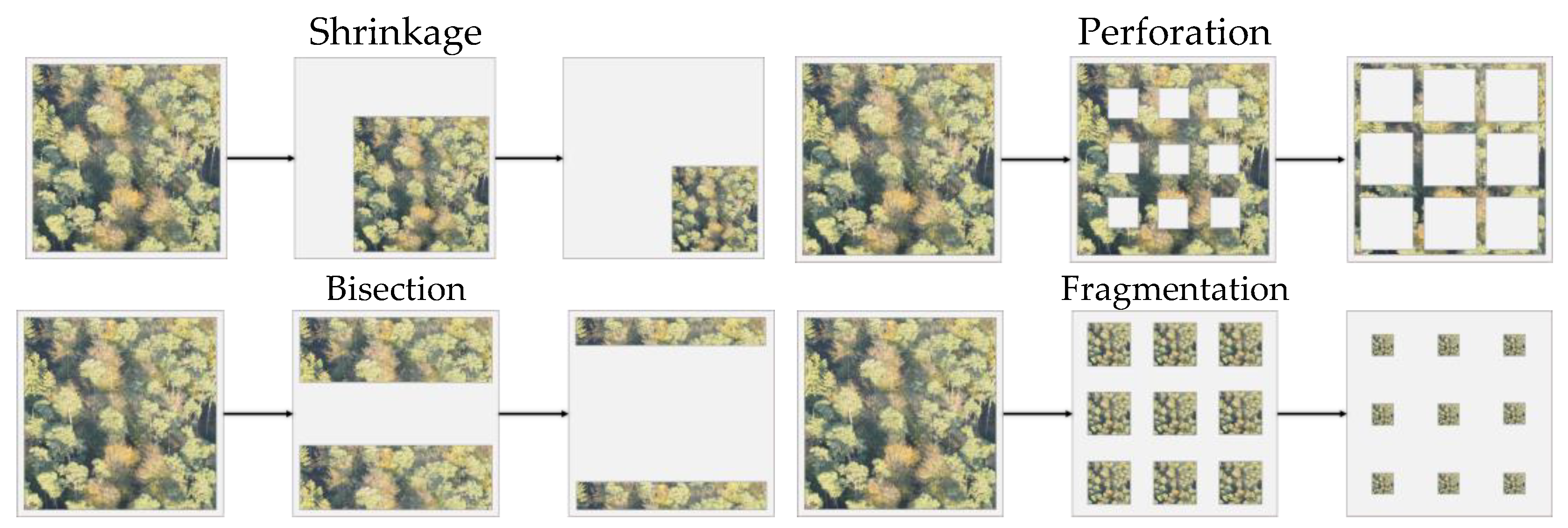
Figure 2.
Fragmentation without forest loss. Forest patches are more numerous in the subsequent frames; however, the overall area of forest within the landscape is unchanged. Adapted from [16].
Figure 2.
Fragmentation without forest loss. Forest patches are more numerous in the subsequent frames; however, the overall area of forest within the landscape is unchanged. Adapted from [16].
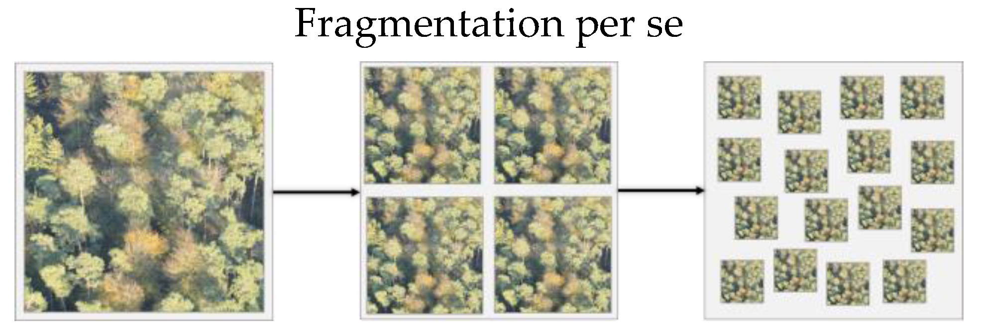
Figure 3.
A mature forest perimeter where tree architecture has developed according to abiotic to conditions along the forest perimeter (A). Recently disturbed perimeters expose spruce stems to increased sunlight, wind, and temperatures (B, C).
Figure 3.
A mature forest perimeter where tree architecture has developed according to abiotic to conditions along the forest perimeter (A). Recently disturbed perimeters expose spruce stems to increased sunlight, wind, and temperatures (B, C).
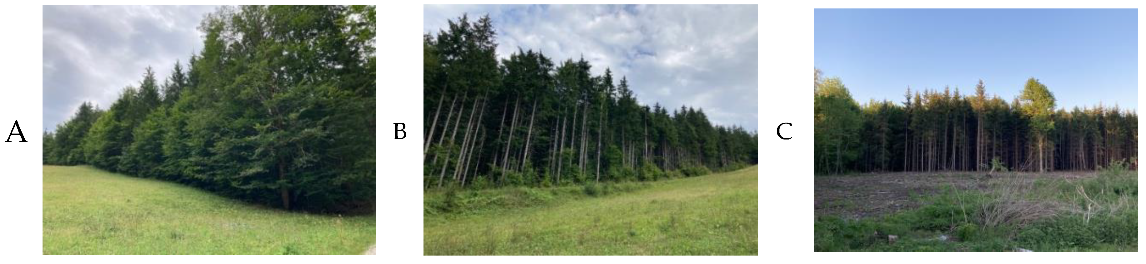
Figure 4.
Simplified examples of fragmentation patterns with polygons outlined. Numerous small patches have no distinct core zone (A), variation in patch shapes (simple/geometric, linear, highly complex) (B), perforations within forests result in longer perimeters and exposure to increased sunlight, temperature, and wind (C), large continuous forests have a distinctive buffer region (100m, blue); the ‘edge’, and interior (orange); the ‘core’, which can support greater number of species (D), linear patches can act as corridors to support animal movement (purple), meanwhile decreased connectivity between patches can have species-specific impacts on animal movement and migration (green) (E). Adapted graphics are courtesy of the University of Maryland (Center for Environmental Science, Integration and Application Network) Media Library, CC BY-SA [29].
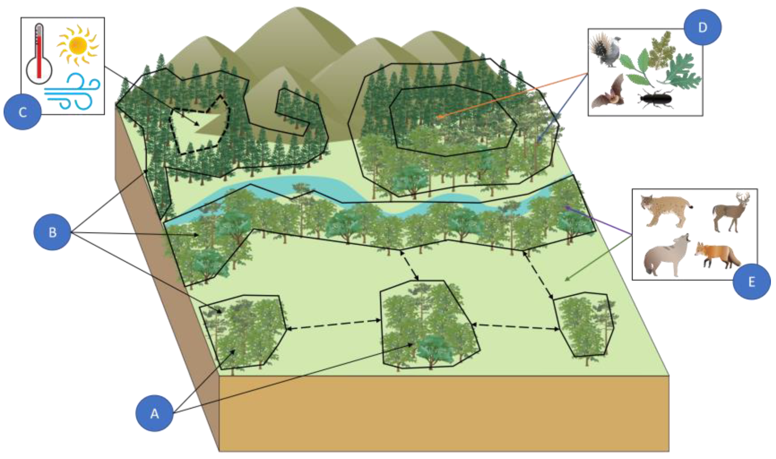
Figure 5.
Overview of Bavaria: Forests and protected areas (A), topography (B), forest ownership (C) and climate (D, E). Adapted from [34].
Figure 5.
Overview of Bavaria: Forests and protected areas (A), topography (B), forest ownership (C) and climate (D, E). Adapted from [34].
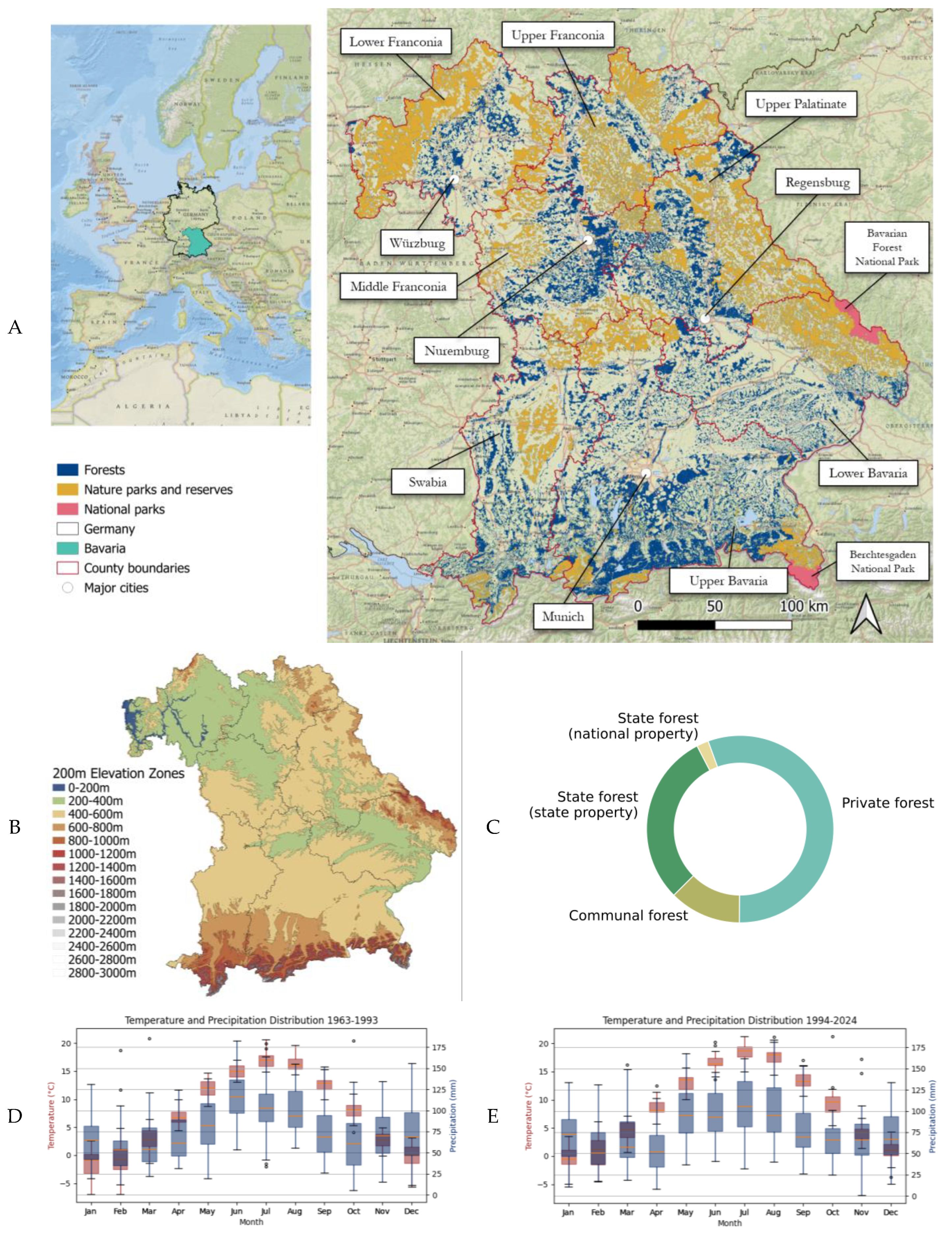
Figure 6.
Summary of workflow.
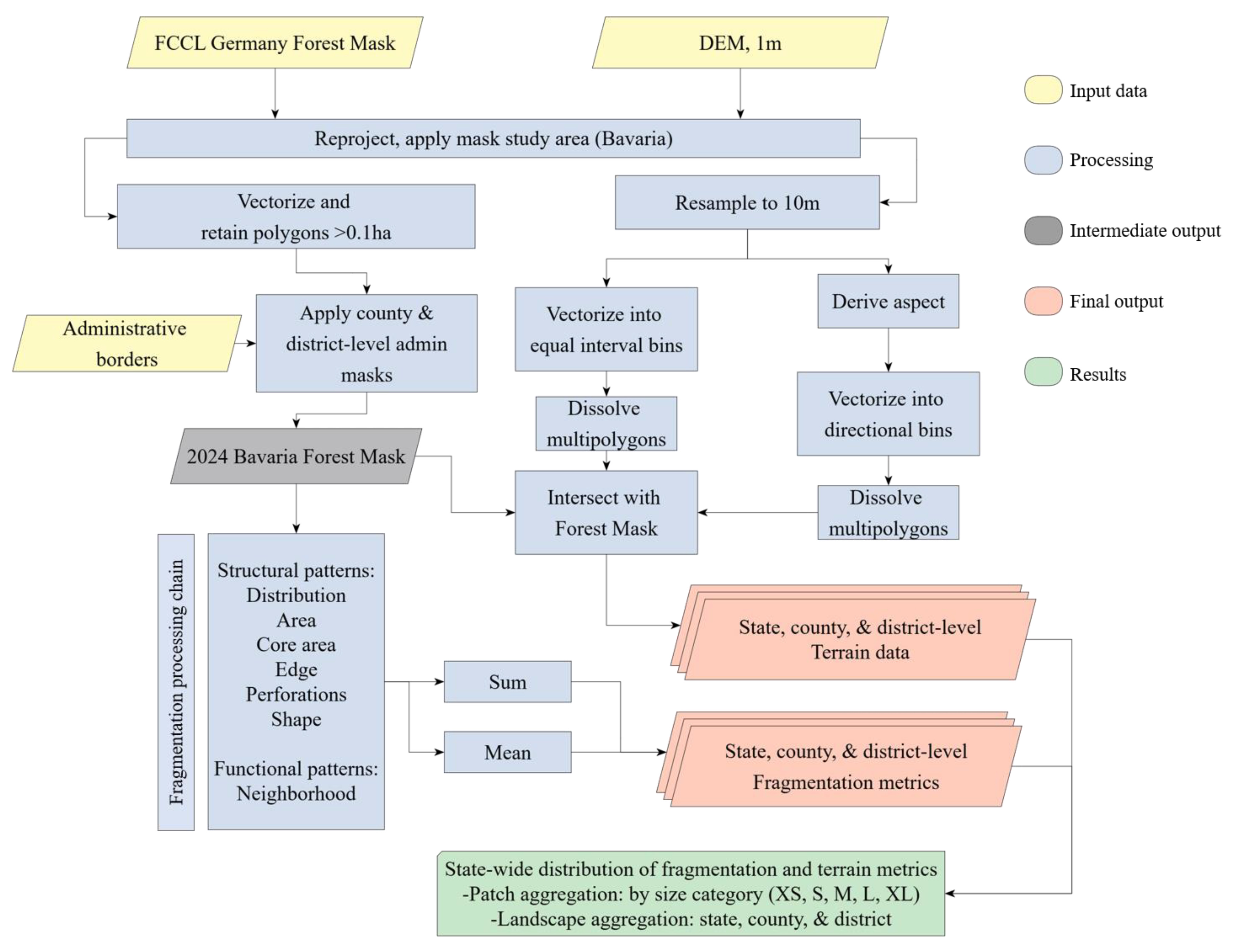
Figure 7.
Log-transformed distribution of patch sizes. Small patches are over represented in the dataset.
Figure 7.
Log-transformed distribution of patch sizes. Small patches are over represented in the dataset.
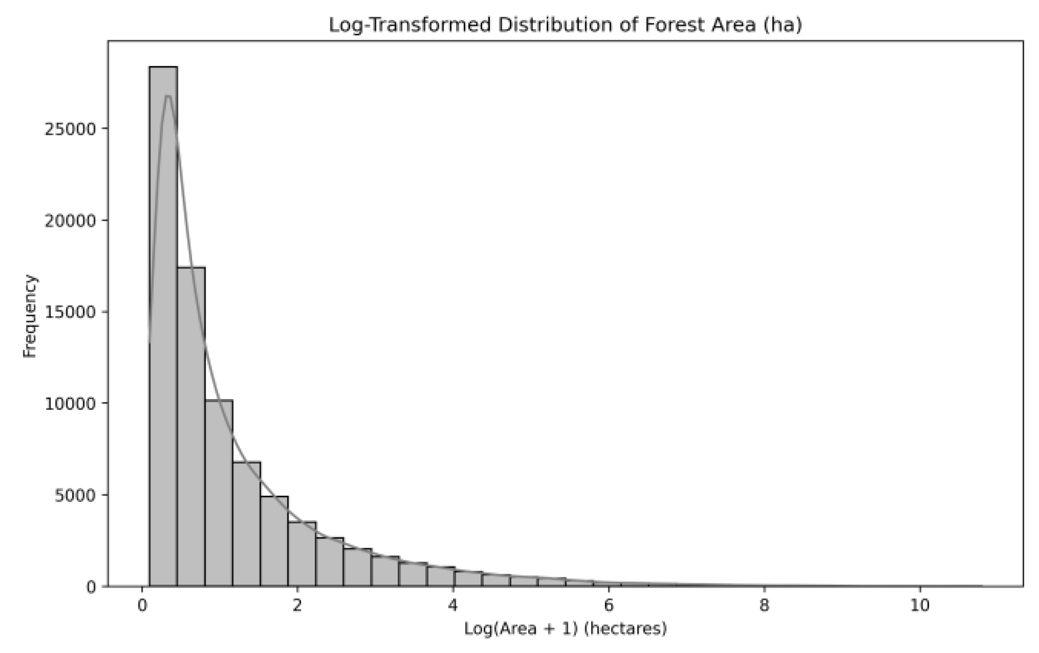
Figure 8.
Overview of forest patch size and distribution (A). Elevations less than 600 m.a.s.l comprise the majority of area in the state, however forest cover is highest at elevations between 800-1400 m.a.s.l. (B). Most hillsides are oriented to the south, however east-facing slopes account for the highest forest cover (C).
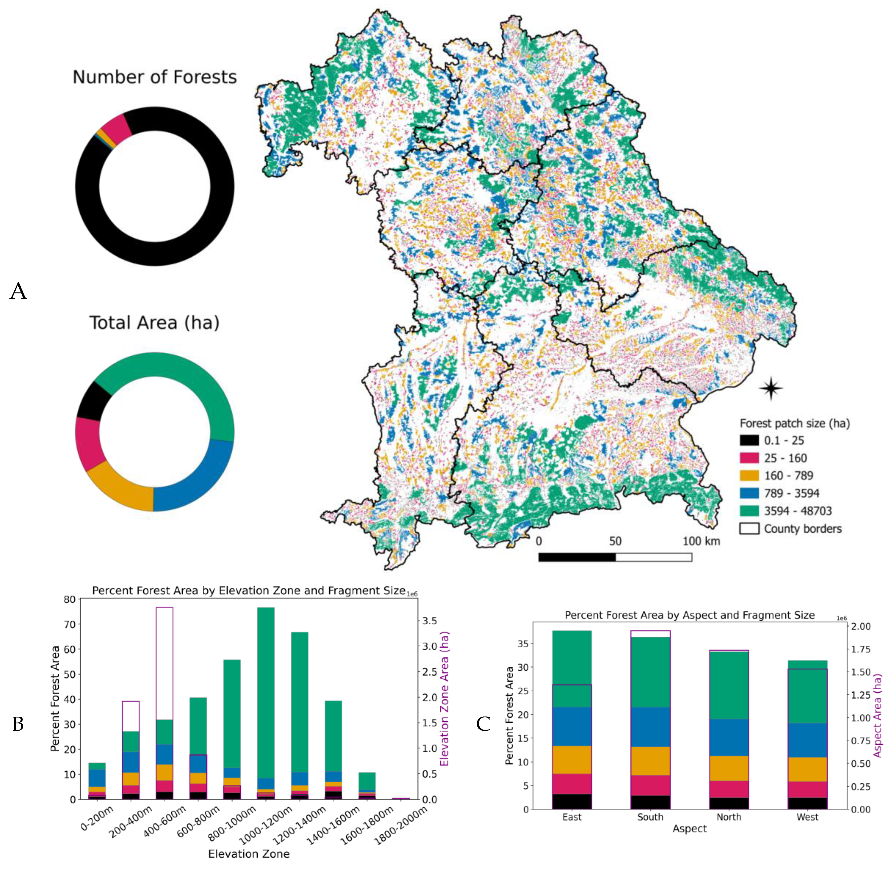
Figure 9.
Comparison of fragmentation metrics across fragment size categories.
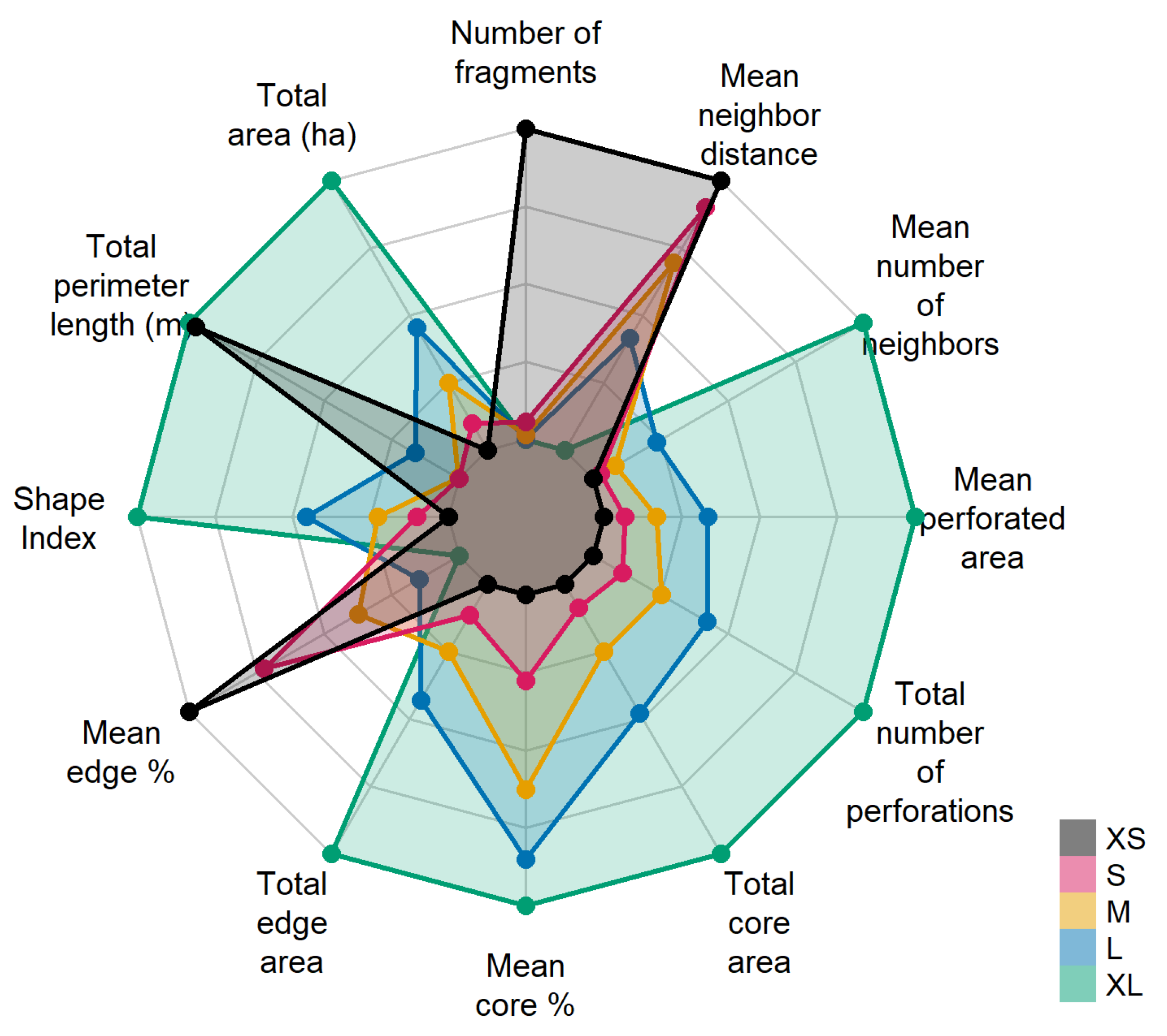
Figure 10.
Examples of increasing values of the shape complexity metric: 1.2 (A), 2.3 (B), 4.0 (C), 5.7 (D), 6.3 (E, e), 8.0 (F, f), 15.0 (G, g), 60.0 and (H, h). Values close to 1 indicate basic geometric shapes whereas high values indicate highly complex shapes which include perforations. Dark green represents core forest area while lavender represents the edge area at a depth of 100m.
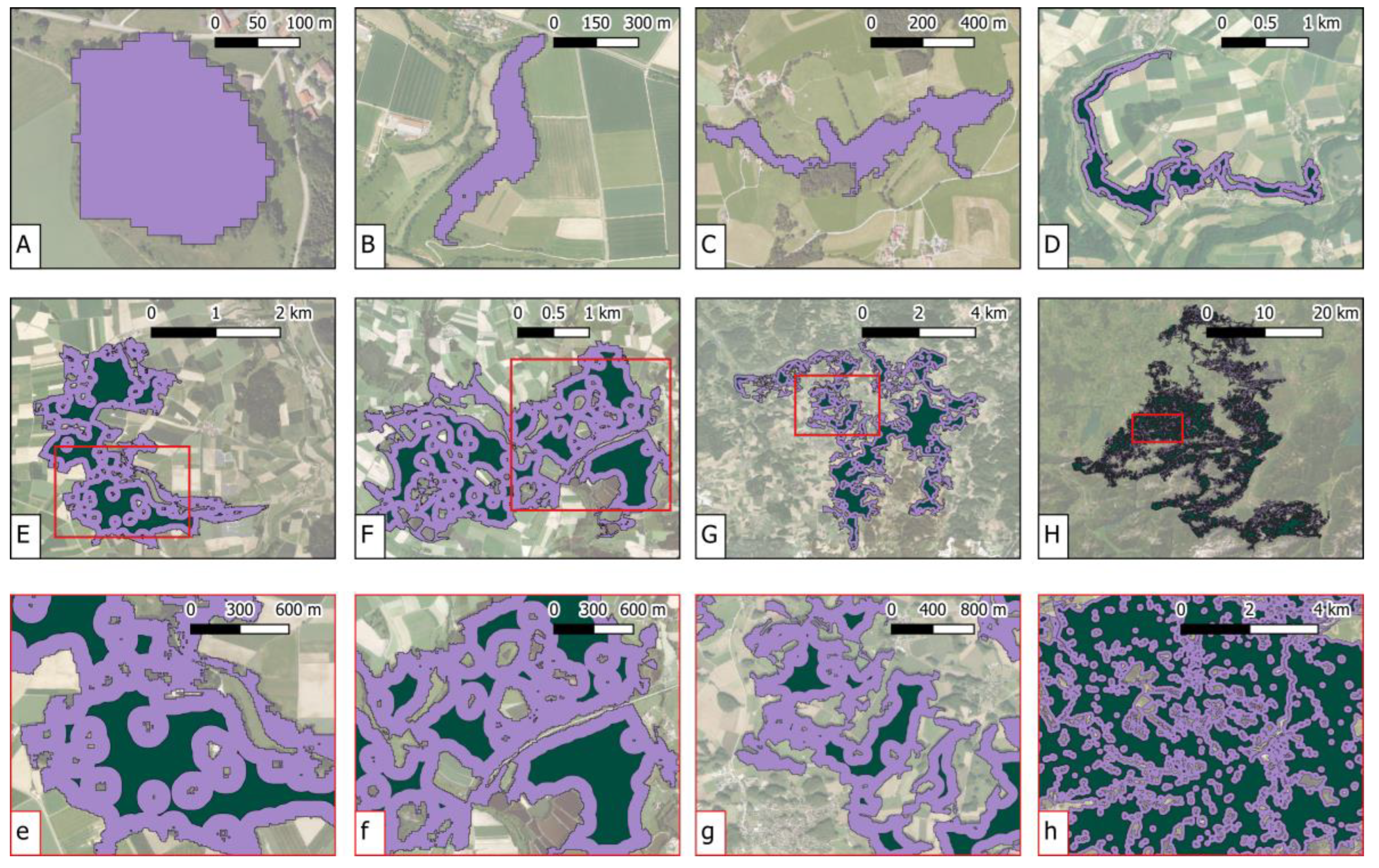
Figure 11.
Spatial distribution of selected fragmentation densities.
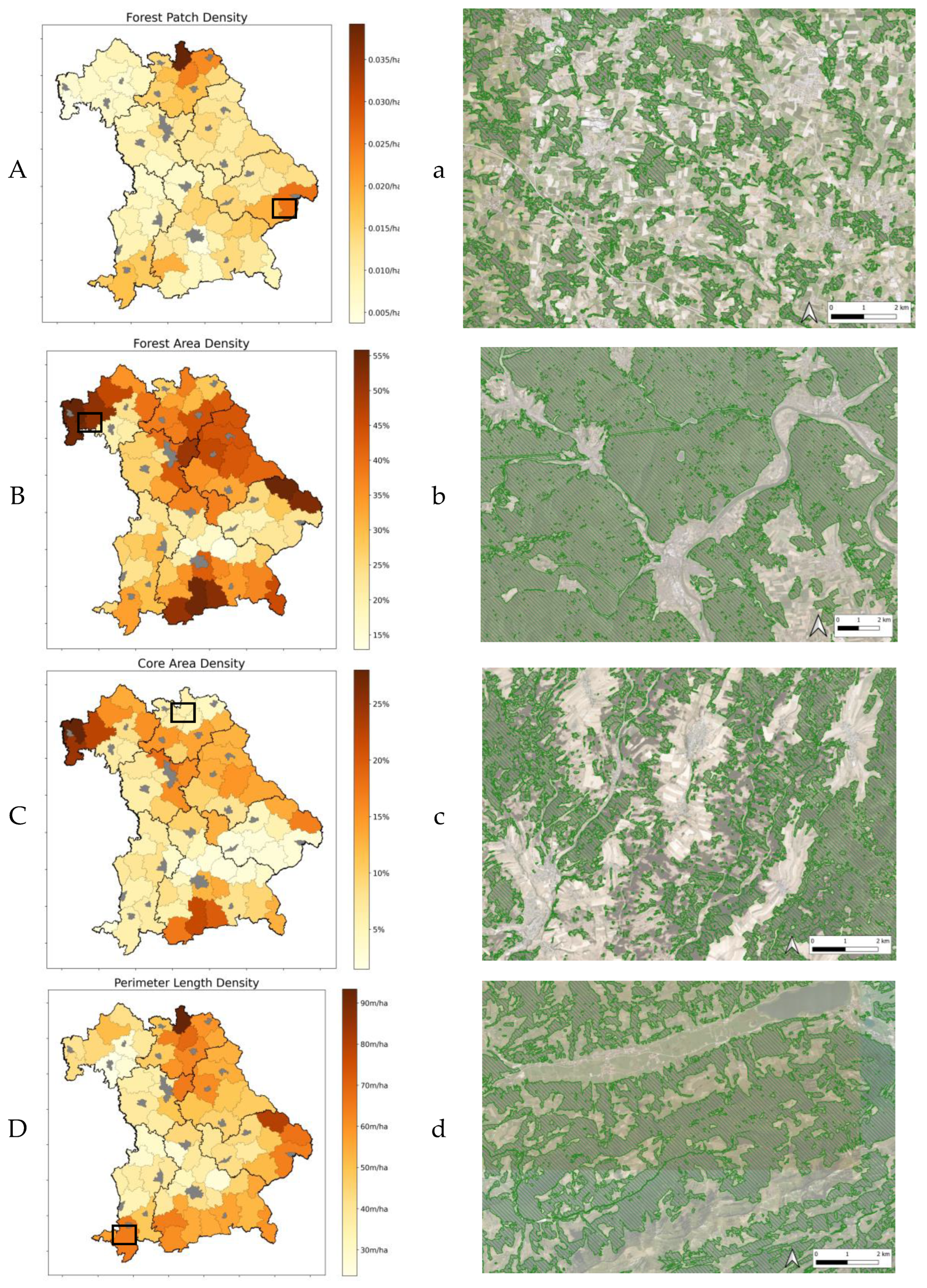
Figure 12.
Spatial distribution of selected fragmentation densities.
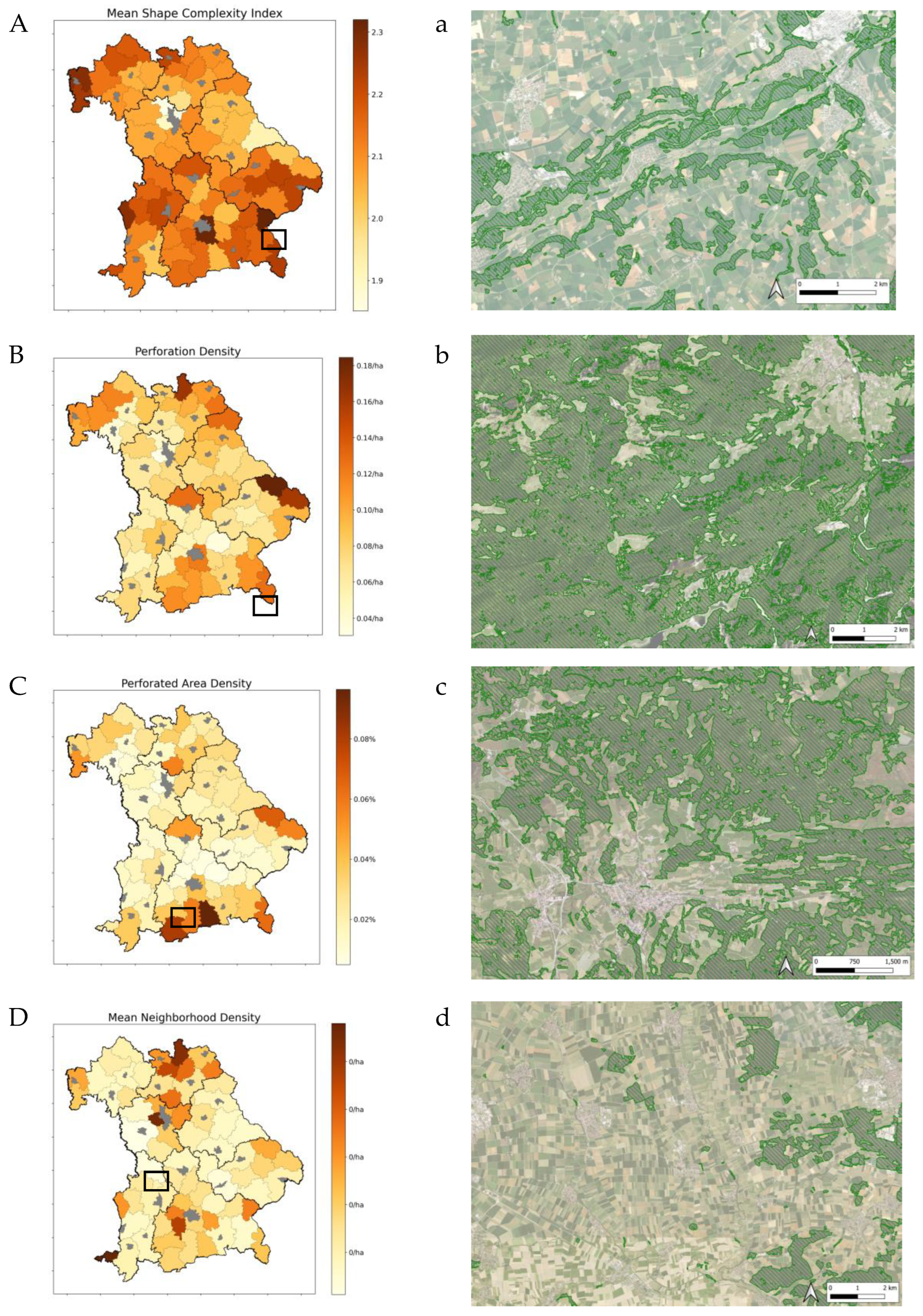
Table 1.
Fragmentation intensity based on forest amount relative to the number of fragments.
| Forest area | Number of fragments | Interpretation | Fragmentation |
| High | Low | Fragmentation intensity is low, forests likely have larger core areas | Low |
| High | High | Fragmentation per se is high however, forest amount is preserved | Moderate to high |
| Low | Low | Forest is aggregated but scarce or potentially isolated | Low to moderate |
| Low | High | Intense fragmentation, forest areas are scarce and disaggregated | High |
Table 2.
The number of neighbors and the distance between patches can conceptualize how isolated or aggregated forest patches are within a landscape.
Table 2.
The number of neighbors and the distance between patches can conceptualize how isolated or aggregated forest patches are within a landscape.
| Number of neighbors | Distance to neighbors | Interpretation | Aggregation |
| High | Low | Fragmentation intensity is high but patches are less isolated | High |
| High | High | Fragmentation is high, and patches are more isolated or dispersed | Low to moderate |
| Low | Low | Fragmentation is low and patches are tightly aggregated | Moderate to high |
| Low | High | Patches are few and quite isolated | Low |
Table 4.
Datasets used.
| Dataset | Description | Type | Spatial resolution | Author | Pub. Date | Access |
| Forest Canopy Cover Loss (FCCL) Forest Mask | Detection based on Disturbance Index (DI) | Raster | 10m | Thonfeld et al. | 2025 | DLR geoservice, https://doi.org/10.15489/ef9wwc5sff75 |
| Digital elevation model (DEM) | High-resolution DEM based on ALS data | Raster | 1m | Bavarian Surveying Authority | Bavarian Geoportal, www.geoportal.bayern.de |
Table 5.
Description of fragmentation metrics.
| Landscape pattern | Category | Metric (aggregation) | Unit | Description or formula | Interpretation |
| Structural | Distribution | Number of patches (sum) | n/a | The total number of patches within a given landscape or administrative unit | High values suggest discontinuous forest within a given landscape. |
| Structural | Area | Area (sum, mean) | Hectares | Area of forest patch(es) | Higher values suggest more continuous forest when number of patches is low. |
| Structural | Core Area | Core area (sum, mean) | Hectares | Core forest area considering an edge depth of 100m | Value indicates size of core forest. |
| Core area % (mean) | Hectares | Percent of core area, considering an edge depth of 100m | High values suggest a higher ratio of core to edge area. | ||
| Structural | Edge | Perimeter (sum, mean) | Meters | Patch perimeter length | High values suggest greater exposure to edge effects. |
| Edge area (sum, mean) | Hectares | Edge depth (100m) is a measure of the region of forest from the perimeter edge toward the core area | Trees inside edges experience higher sunlight, wind, temperatures and drier soil conditions. | ||
| Edge area % (mean) | n/a | The ratio of edge area (100m edge depth) to overall area | Higher values may equate to lower overall core area. | ||
| Structural | Perforations | Number of perforations (sum, mean) | n/a | Number of perforations in a forest patch or landscape | Highly complex patch shapes and increased exposure to edge effects. |
| Perforated area (sum, mean) | Hectares | Area of perforations in a forest or landscape | High values can suggest increases in shape complexity. | ||
| Structural | Shape | Paratio (mean) | n/a | Higher values equate to higher shape complexity (varies with size of patch). | |
| Shape index (mean) | n/a | Higher values equate to higher shape complexity (employs a constant to correct for size). | |||
| Functional | Neighbor-hood | Number of neighbors (sum, mean) | n/a | Counts neighboring forests based on edge-to-edge distance within 200m buffer of each patch. | Increases over time can indicate higher fragmentation intensity. |
| Area of neighbors (sum, mean) | Hectares | Area of neighboring patches within 200m buffer. | High values indicate large nearby forests. |
Disclaimer/Publisher’s Note: The statements, opinions and data contained in all publications are solely those of the individual author(s) and contributor(s) and not of MDPI and/or the editor(s). MDPI and/or the editor(s) disclaim responsibility for any injury to people or property resulting from any ideas, methods, instructions or products referred to in the content. |
© 2025 by the authors. Licensee MDPI, Basel, Switzerland. This article is an open access article distributed under the terms and conditions of the Creative Commons Attribution (CC BY) license (http://creativecommons.org/licenses/by/4.0/).
Copyright: This open access article is published under a Creative Commons CC BY 4.0 license, which permit the free download, distribution, and reuse, provided that the author and preprint are cited in any reuse.


