
Submitted:
21 November 2025
Posted:
25 November 2025
You are already at the latest version
Abstract
Quantum Informational Relativity (QIR) proposes a unified formalism in which microphysical dynamics, spacetime structure, and cosmological evolution are consistently derived from an underlying informational field-theoretic framework. This monograph consolidates the complete formulation of QIR from the operator-level action and classical limit to the Hamiltonian structure, consistency relations, and effective constants and organizes it into a coherent, self-contained theory. At the microscopic level, QIR predicts informational solitons, canonical fluctuation modes, confinement, mass generation, and small but measurable shifts in Standard Model observables. A Wilsonian mapping links these scales to cosmology, producing a smooth continuation across 30+ orders of magnitude. Cosmologically, QIR generates percent-level deviations in the growth function and lensing potential, easing the S8 tension while leaving background distances unchanged. Fully nonlinear N-body simulations performed with a modified SWIFT engine confirm these signatures and reproduce realistic cosmic structures. Altogether, this work provides the first complete exposition of QIR as a mathematically consistent, observationally testable, and scale-continuous alternative to standard microphysical and gravitational dynamics.
Keywords:
quantum informational relativity
; informational field theory
; operator-valued fields
; canonical quantization
; solitonic dynamics
; topological sectors
; effective field theory
; modifiedgravity
; large-scale structure
; weak lensing
; growth function
; N-body simulations
; scale continuity
; microphysical–cosmological correspondence
Notations and Conventions
This monograph employs both classical and operator-valued structures. To ensure full clarity, we fix from the outset a strict and unambiguous distinction between classical fields, quantum operators, canonical variables, effective quantities, and geometric objects.
Classical and Quantum Quantities
We use the following global convention:
- Classical objects carry no hat:
- Operator-valued objects carry a hat:
- The spacetime metric and curvature tensors are treated as classical throughout the theory and therefore never carry a hat.
- Expectation values in the QIR Hilbert space are written
Normal ordering is assumed for all operator expressions involving unless stated otherwise.
Canonical Quantization
The conjugate momentum operator is defined by
Equal-time canonical commutation relations are
Canonical Normalization of Fluctuations
Fluctuations around a background configuration are written
The canonically normalized fields are
with canonical equal-time relations
Mode Expansion
The normalized quantum fluctuation admits the standard decomposition
with
Internal Multiplets and Topological Sectors
When internal structure is required, we extend
with operator counterpart . Phase maps and winding structures used for particle classification are always defined using the normalized multiplet.
Spacetime and Geometry
We work on a Lorentzian manifold with signature . Indices are raised and lowered with . Curvature tensors follow
Informational Modulation
Classically,
The operator version is
The effective local light speed is
Physical and Effective Metrics
The physical metric is . An auxiliary effective metric is occasionally used:
but all gravitational dynamics are defined with .
Energy–Momentum Tensors
Matter: (classical). Informational:
Total conservation:
Einstein Equation (QIR Form)
Units
Natural units are assumed. The factor is kept explicit to track informational modulation.
Fourier Transform
Functional Derivatives
These conventions remain fixed throughout the monograph unless explicitly overridden for specific calculations.
1. Introduction
The search for a unified description of microphysical dynamics, spacetime geometry, and cosmological structure formation remains one of the central challenges in contemporary theoretical physics. Quantum field theory (QFT) successfully describes local excitations and particle interactions, while General Relativity (GR) governs the large-scale curvature of spacetime. Yet the conceptual foundations of these frameworks differ profoundly: QFT is rooted in operator-valued fields defined on a fixed background, whereas GR treats geometry itself as dynamical. Reconciling these perspectives has proven difficult, not only at the level of mathematical consistency, but also in terms of identifying a common set of underlying physical principles.
A recurring idea in several approaches to unification is that spacetime, fields, or interactions may arise from deeper informational, statistical, or emergent structures. These perspectives appear in contexts ranging from entanglement-based derivations of geometry to thermodynamic formulations of gravitational dynamics. While diverse in implementation, they share the notion that traditional geometric and quantum concepts might both originate from an informational substrate.
Quantum Informational Relativity (QIR) develops this line of thought in a specific and operationally well-defined manner. The central dynamical entity is an informational field whose modulation factor affects inertial, interaction, and gravitational responses while preserving relativistic covariance. In this view, particles, interactions, and geometric curvature are not independent ingredients but manifestations of a single informational degree of freedom. The resulting structure retains the full tensorial and geometric content of GR, yet introduces a controlled and covariant deformation through the informational sector.
A distinctive feature of QIR is that informational fluctuations, their canonical normalization, and their topological properties naturally give rise to microphysical structures such as stable localized excitations, phase sectors, and emergent mass scales. At the opposite end of the spectrum, the same informational coupling modifies the growth of cosmic structures and the lensing potential at late times, providing a possible explanation for the mild yet persistent tension between weak-lensing surveys and CDM predictions. Because the underlying modulation is the same at all scales, QIR establishes a continuous bridge between microphysical and cosmological regimes without introducing additional free parameters.
Beyond analytic calculations, the informational modification can be implemented directly in N-body simulations, allowing nonlinear structure formation to be tested in fully dynamical settings. This provides an essential consistency check: any viable extension of GR must recover realistic halo distributions and large-scale structures while remaining compatible with observed growth suppression.
The purpose of this monograph is twofold. First, it presents a complete and self-contained construction of QIR, from the operator-level action and canonical quantization to geometric consistency and scale transitions. This includes full derivations and explicit intermediate steps, ensuring mathematical transparency. Second, it synthesizes the observational and phenomenological consequences across microphysical, cosmological, and nonlinear regimes, demonstrating how a single informational field can produce coherent physics over many orders of magnitude.
The document is organized as follows. Section 2 develops the foundational operator structure of QIR, including the fundamental action, the informational stress tensor, the unified Einstein equation, the Hamiltonian formulation, canonical normalization, and the derivation of effective propagation and coupling scales. Section 3 presents the quantization of the informational field, including operator canonical quantization, mode expansion on curved backgrounds, the propagator, spectral decomposition, renormalized quantum observables, and the vacuum structure. Section 4 confronts the microphysical predictions of QIR with high-energy data, examining informational corrections, decay processes, scattering cross sections, spectral signatures, informational mixing, and combined collider constraints. Section 5 develops the cosmological sector, including background evolution, linear growth, weak lensing, CMB constraints, nonlinear structure formation, and unified cosmological tests. Section 6 presents the numerical validation using SWIFT, including the simulation pipeline, growth extraction, matter power-spectrum evolution, cosmic-web classification, velocity-field diagnostics, and global nonlinear validation. Section 7 investigates astrophysical and propagation signatures across gravitational potentials, halo dynamics, radiation transport, time-delay effects, and high-energy propagation. Section 8 provides a general discussion and comparative assessment of QIR, including structural synthesis, physical interpretation, internal consistency, comparisons with GR, CDM, and modified gravity, limitations, and falsifiable predictions. Section 9 concludes the monograph.
2. Foundational Action and Operator Structure
The Quantum Informational Relativity (QIR) framework is built upon a single informational operator field whose local amplitude modulates inertial, geometric, and coupling strengths through a dimensionless informational modulation function . The goal of this section is to establish rigorously the full operator-level dynamical structure: the fundamental action, its variations with respect to the metric and the informational field, the unified Einstein equation, and the covariant canonical quantization of . All quantities are written in the physical g-frame unless explicitly stated.
2.1. Fundamental Operator Action
The Quantum Informational Relativity (QIR) framework is grounded in the postulate that the fundamental dynamical entity is an operator-valued informational field defined on a Lorentzian manifold . Its amplitude encodes local informational density, and its variations renormalize inertial and geometric responses through a positive definite, dimensionless modulation function .
In this subsection we construct the fundamental action, justify its operator structure, and examine its mathematical properties. We proceed step by step to make explicit the assumptions, domains of definition, and the covariant identities needed for the derivations that will follow in subsequent subsections.
2.1.1. Principles Guiding the Action
The informational field is assumed to satisfy the following general principles:
- Covariance: all dynamical quantities must transform as well-defined geometric objects under diffeomorphisms.
- Positivity: the informational modulation must be everywhere positive to ensure a well-posed kinetic structure and a hyperbolic operator equation of motion.
- Hermiticity: the action must be self-adjoint in the Hilbert space ; this ensures that energies, momenta, and stress tensors are real-valued expectation values.
- Minimal coupling: the covariant derivative includes the Levi-Civita connection of , and possibly internal gauge connections acting on multiplet extensions of .
- Locality: the action depends on and its first derivatives only, consistent with standard field-theoretic structure.
These principles uniquely restrict the admissible form of the action.
2.1.2. Construction of the Operator Action
Let be an operator-valued scalar field acting on the QIR Hilbert space . The most general diffeomorphism-invariant, Hermitian, local action built from , , and up to mass dimension four is
where and are operator-valued functions defined as power series in . Hermiticity requires to be a real, positive, even function.
The essential feature of QIR is the identification
where is the informational modulation governing inertial and coupling strength.
2.1.3. Informational Modulation and Its Properties
The modulation function encodes how the local informational density renormalises all dynamical responses. For consistency, it must satisfy:
- for all admissible states, ensuring positivity of the kinetic operator.
- is a self-adjoint operator function, i.e. .
- must commute with scalars but not necessarily with itself unless is taken to be Hermitian.
A widely used form is
which is positive and even. However, our derivations remain valid for any differentiable operator function .
2.1.4. Final Form of the Operator Action
With the above identifications, the fundamental QIR action is
The potential is chosen to be a real, bounded-from-below, self-adjoint operator function. A common example is
though nothing in the subsequent derivations depends on this specific form.
2.1.5. Hermiticity and Operator Ordering
Because and may not commute, care must be exercised in the definition of . Two choices are common:
- Symmetric ordering:
- Left ordering:
QIR chooses the symmetric ordering to guarantee strict Hermiticity. Thus we interpret the kinetic term in (2) as
In the semiclassical limit , the two orderings coincide, ensuring consistency with classical dynamics.
2.1.6. Domain of the Covariant Derivative
The operator derivative acts as
where is either:
- the Levi-Civita connection acting on tensors (trivial for scalars),
- an internal gauge connection acting on multiplets , .
Thus for a scalar operator,
but when internal indices are present,
All subsequent variations of assume these transformation rules.
2.1.7. Classical Limit and Emergent Interpretation
Taking expectation values in a suitable state gives
and the action reduces to its classical version:
This classical limit recovers all the expressions used in microphysical and cosmological analyses.
This concludes the full construction, motivation, and operator-level justification of the fundamental QIR action. The next Section 2.2 performs the complete metric variation, including the explicit treatment of
and leads to the fully derived informational stress tensor and the geometric sector of the unified field equations.
2.2. Metric Variation and the Informational Stress Tensor
In this section we perform the complete variation of the operator action (2) with respect to the metric . This derivation is essential because it produces the informational energy–momentum tensor and establishes its role in the unified Einstein equation.
The variation involves multiple tensorial identities, variations of the determinant, inverse metric, and Christoffel symbols, as well as the metric dependence of the covariant derivative acting on . For full transparency, every required identity is derived explicitly.
2.2.1. Variation Identities for the Metric
We begin with standard results from differential geometry.
Inverse Metric
Since , variation gives
Determinant
Starting from , one obtains
Christoffel Symbols
The Levi-Civita connection varies as
Variation of the Covariant Derivative Acting on
For a scalar operator-valued field ,
For a multiplet with gauge connection ,
because does not depend on the metric.
2.2.2. Varying the Kinetic Term
The kinetic term of the action is
Its variation is
Lowering indices on yields
Thus
2.2.3. Variation of the Potential Term
The potential term is
Since does not depend on the metric,
2.2.4. Total Metric Variation of the Action
Collecting the kinetic and potential variations,
we obtain
Recognizing
we rewrite the expression in the standard form
where the informational stress tensor is identified as
This is the fully derived, operator-level informational energy–momentum tensor.
2.2.5. Symmetry and Hermiticity
Because the action is diffeomorphism invariant and defined with symmetric operator ordering, satisfies:
- Symmetry: .
- Self-adjointness: .
- Covariant conservation (proved later): is related to the field equation.
These guarantees follow from Noether’s theorem applied to diffeomorphism invariance, but the conservation statement will be established explicitly in Section 2.4.
2.2.6. Classical Limit
Replacing the operator with its expectation value gives
which is the informational tensor used in microphysical and cosmological applications.
This completes the fully explicit metric variation. The next Section 2.3 performs the complete field variation, leading to the operator-level informational equation of motion, including all intermediate steps and operator-ordering corrections.
2.3. Variation with Respect to the Informational Field
We now perform the full variation of the action (2) with respect to the operator field and its adjoint . Unlike traditional scalar field variations, the present case requires special care due to the presence of:
- operator-valued functions and ;
- non-commutativity between , , and derivative operators;
- the metric-dependent contraction .
To guarantee Hermiticity of the resulting equations, we vary and independently and combine the expressions at the end.
Throughout this subsection, boundary terms are explicitly evaluated and discarded under the assumption that variations vanish on the boundary of the integration domain.
2.3.1. Structure of the Variation
From (2), the variation with respect to is
This expression contains three types of variations:
We compute each contribution separately.
2.3.2. Variation of the Modulation Function
Since is an operator function, its variation is
where is defined by its power-series expansion (Fréchet derivative).
The contribution to the action is therefore
Because and do not commute in general, we keep this ordering explicit.
2.3.3. Variation of the Covariant Derivative
For a scalar operator field, the covariant derivative simplifies to
Hence
The contribution to the action becomes
Integrating by parts,
boundary terms vanish because the variation is assumed to vanish on .
2.3.4. Variation of the Potential
The variation of the potential term is straightforward:
2.3.5. Combined Variation and Euler–Lagrange Equation
Combining all contributions,
Factoring out gives
where the operator Eulerian is
Requiring yields the operator equation of motion:
By Hermiticity, the variation with respect to yields the conjugate equation.
2.3.6. Covariant Form
Using the identity
the equation can be written in explicitly geometric form:
2.3.7. Classical Limit
Replacing the operator field by its expectation value gives
For the common form
the equation becomes
2.3.8. Interpretation
The informational field equation exhibits two key features:
- The principal term defines a modulated wave operator whose magnitude depends on informational density.
- The nonlinear drift term has no analogue in canonical scalar field theory and captures the self-interaction of informational inertia.
These two ingredients are responsible for:
- the emergence of microphysical excitations,
- the existence of solitonic sectors,
- the scale-dependent propagation speed,
- the coupling between informational content and curvature.
This completes the full operator-level variation with respect to . The next Section 2.4 establishes the fully derived unified Einstein equation, including an explicit proof of covariant conservation.
2.4. Unified Einstein Equation with Informational Coupling
Having obtained the informational tensor and the operator equation of motion for , we now derive the full gravitational dynamics of QIR. The key result is the unified Einstein equation, which relates the geometric curvature to the combined informational–matter tensor, modulated by the informational function .
This subsection provides a complete derivation:
- variation of the Einstein–Hilbert term,
- combination with the informational and matter variations,
- extraction of the field equation,
- proof of covariant conservation using the Bianchi identity,
- discussion of the local renormalisation of coupling scales.
2.4.1. Variation of the Einstein–Hilbert Action
The Einstein–Hilbert action is
Its variation is classical:
where is the usual boundary term
Assuming appropriate boundary conditions,
2.4.2. Total Metric Variation of the Full Action
The full gravitational-informational-matter action is
We have already obtained:
and
where is the operator energy–momentum tensor of matter.
Thus the total variation is
Requiring stationarity for arbitrary gives
Multiplying both sides by yields:
Next we incorporate the informational renormalisation of the effective speed of light.
2.4.3. Informational Renormalisation and Effective Coupling
In QIR the local speed of light is given by
The combination that naturally appears in gravitational theory therefore becomes
Reabsorbing this factor into the right-hand side of (33) yields the informationally renormalised Einstein equation:
This is the fundamental operator-level gravitational equation of Quantum Informational Relativity.
2.4.4. Proof of Covariant Conservation
To establish dynamical consistency, we must prove:
Step 1: Bianchi identity
The twice-contracted Bianchi identity states:
Applying to (34),
Because depends only on Z, and acts on fields but not on the metric, the prefactor behaves as a scalar function under :
But since
we obtain
Thus the prefactor is covariantly constant.
Step 2: Result
Therefore
which is exactly (35).
This conservation law is the geometric manifestation of the equation of motion for , as we now show.
2.4.5. Equivalence with the Field Equation
Substituting the explicit form of into the conservation law and expanding each term leads (after cancellation of several gradient contributions) precisely to the operator field equation derived in Section 2.3:
Thus:
- the Einstein equation enforces the informational field equation,
- the informational field equation ensures consistency of the Einstein equation.
This mutual implication is analogous to the relationship between matter conservation and the Einstein field equations in standard GR, but now extended to the informational sector.
2.4.6. Classical Limit
The classical limit of the unified Einstein equation is
where is the classical informational tensor and the standard matter tensor.
This form underlies all macroscopic applications of QIR, from cosmological evolution to gravitational lensing and dynamical mass profiles.
2.4.7. Interpretation
The unified Einstein equation exhibits the following structural features:
- Informational modulation. The factor acts as a state-dependent modification of gravitational coupling.
- Local renormalisation. The combinationeffectively defines a local gravitational coupling .
- Self-consistency. Conservation of the combined informational–matter tensor follows automatically from geometric consistency.
- Operator structure. The equation remains valid at the operator level, with physical predictions recovered via expectation values or classicalisation.
This completes the full derivation of the unified Einstein equation in Quantum Informational Relativity. The next Section 2.5 constructs the covariant canonical momentum, the Hamiltonian, and the ADM (3+1) decomposition required for quantisation and dynamical analysis.
2.5. Conjugate Momentum and Hamiltonian Structure
In this subsection we construct the full canonical structure associated with the informational field . The derivation proceeds in three stages:
- construction of the covariant conjugate momentum ,
- derivation of the covariant Hamiltonian density,
- ADM decomposition and explicit Hamiltonian constraints.
This structure prepares the ground for quantisation in Section 3.
2.5.1. Covariant Conjugate Momentum
The Lagrangian density extracted from (2) is
The covariant conjugate momentum operator is defined as
and similarly
For clarity we keep the factor explicit. When both momenta appear in the Hamiltonian these factors combine naturally.
2.5.2. Covariant Hamiltonian Density
The covariant Hamiltonian density is defined as
Using symmetric ordering,
Thus the Hamiltonian becomes
Hence:
This is the covariant energy density of the informational field.
2.5.3. ADM Decomposition
We now decompose spacetime into spacelike hypersurfaces with induced metric , lapse N, and shift . The line element is
The inverse metric is
For a scalar operator field,
Thus:
Using the metric, the kinetic structure decomposes as:
2.5.4. Canonical Momentum in ADM Variables
Using (40):
The momentum conjugate to on the hypersurface is
Similarly
2.5.5. ADM Hamiltonian Density
The ADM Hamiltonian density is defined as
Using
we obtain after substitution and simplification:
where
is the momentum constraint density.
2.5.6. Hamiltonian and Momentum Constraints
The Hamiltonian constraint is obtained from the coefficient of the lapse:
The momentum constraint is obtained from the coefficient of the shift:
These constraints are the generators of diffeomorphisms within the hypersurface and normal to it.
2.5.7. Classical Limit
Replacing operators by their expectation values gives the classical Hamiltonian:
The informational factors Z and appear naturally:
- Z multiplies the spatial gradient term (inertia of geometry), - multiplies the kinetic term (inertia of the informational excitation).
2.5.8. Interpretation
The ADM Hamiltonian displays two characteristic signatures of QIR:
- Dual inertia structure. The combinationshows that excitations become lighter or heavier depending on informational density.
- Geometric–informational coupling. The factor links informational gradients directly to spatial curvature.
- Constraint structure identical to GR. Hamiltonian and momentum constraints retain their geometric meaning, guaranteeing full diffeomorphism invariance.
This completes the construction of the canonical and Hamiltonian structures of the informational field. The next Section 2.6 performs the expansion of the action to second order around a background solution and derives the canonical normalisation of fluctuations, explaining the appearance of in microphysics.
2.6. Canonical Normalization and Second-Order Expansion
To prepare for the quantisation procedure in Section 3, we must expand the informational action to second order in small fluctuations around a background configuration. This analysis yields the canonical normalisation of the excitations and explains why microphysical observables naturally acquire the factor .
We proceed systematically:
- define the background and fluctuation fields,
- expand the kinetic term to quadratic order,
- expand the potential term consistently,
- extract the quadratic operator and diagonalise it,
- identify the canonically normalised field and its effective mass.
Throughout this section we work in the classical limit; the operator case follows by standard ordering rules.
2.6.1. Background–Fluctuation Split
Let be a solution of the classical field equation derived in Section 2.3. We introduce small fluctuations:
The modulation function expands as
with .
2.6.2. Expansion of the Kinetic Term
The kinetic part of the action is
Insert the decomposition (53). We first expand the derivative:
Then:
Now multiply by expanded to second order:
Keeping all terms up to quadratic order in :
The linear terms vanish upon integration because satisfies the background equation of motion. Thus, the quadratic part of the kinetic action is:
2.6.3. Removing Linear Derivative Mixing
The mixed term
can be integrated by parts:
boundary terms vanish.
Thus, the mixed derivative term produces only a mass-like correction. The quadratic kinetic term becomes
where
2.6.4. Expansion of the Potential
The potential expands as:
The linear term vanishes because satisfies the background equation. Thus:
2.6.5 Complete Quadratic Action
Combining kinetic and potential contributions,
where
This is the quadratic Lagrangian for fluctuations.
2.6.6. Canonical Normalization: Emergence of
The kinetic term has a prefactor :
To obtain a canonically normalised field, we define
Then
and the kinetic term becomes
Thus the canonically normalised quadratic action is
with effective mass
2.6.7 Physical Interpretation
The renormalised mass demonstrates explicitly:
Thus:
- In regions where , excitations are lighter. - In regions where , excitations are heavier. - All microphysical scales are rescaled by or .
This factor is the mathematical origin of the renormalisation of:
- masses,
- couplings,
- propagation speeds,
- dispersion relations,
in the informational framework.
This completes the full quadratic expansion and the rigorous derivation of the canonical normalisation. The next Section 2.7 develops the explicit computation of effective constants and propagation speeds, completing the foundational operator structure.
2.7. Effective Constants and Propagation Speed
Having established the canonical structure and quadratic expansion of the informational field, we now derive how informational modulation renormalizes the fundamental constants relevant for both the macroscopic geometric sector and the microscopic excitation sector.
We proceed via a sequence of rigorous derivations:
- extraction of the propagation speed of fluctuations from the quadratic action,
- computation of the effective Newton constant ,
- renormalisation of gauge couplings and other interaction strengths,
- consistency checks linking operator-level structure to canonical normalization.
The results generalize the familiar notion of running couplings to a state-dependent and geometrically integrated scale factor encoded in .
2.7.1. Informational Origin of the Local Propagation Speed
In Section 2.6 we derived the quadratic action for the canonically normalized field :
To extract the propagation speed, we return to the un-normalized fluctuations :
Consider a local inertial frame where
The wave operator acting on is
To bring the time derivative into the canonical form , we observe that the physical propagation speed is:
Thus,
This matches precisely the kinematic identity introduced earlier, now derived rigorously from the quadratic operator structure.
2.7.2. Effective Newton Constant
The unified Einstein equation derived in Section 2.4 is:
Substituting gives:
Thus the effective Newton constant is:
Hence: - in high-informational-density regions (), gravity is weaker; - in low-informational-density regions (), gravity is stronger.
This effect plays a central role in large-scale structure and lensing observables.
2.7.3. Gauge Coupling Renormalisation
Consider a minimally coupled gauge field with canonical action
The physical field couples to through the kinetic normalization of :
If the interaction term is
then after canonical normalization:
Thus the effective coupling is
General interactions of the form acquire factors . This is consistent with the dimensional analysis in the quadratic expansion.
2.7.4. Effective Masses
From Section 2.6, the canonically normalised mass is:
Thus the microphysical mass renormalisation is:
Since Z appears in the denominator: - excitations are lighter at high informational density, - excitations are heavier at low informational density.
2.7.5 Summary Table
We summarize the derived effective constants:

| Quantity | Effective Value |
|---|---|
| Propagation speed | |
| Newton constant | |
| Gauge couplings | |
| Masses |
All renormalisations derive from one universal function , expressing the fact that informational density reshapes both microphysical and macroscopic interactions in a coherent, self-consistent manner.
2.7.6. Interpretation
The following points summarize the physical significance:
- Unification. Gravity, gauge couplings, masses, and propagation speeds are modulated by the same informational factor.
- Scale dependence. Unlike RG running, the modulation depends on the local state rather than energy scale.
-
Geometry–information interplay. Because and , informationally dense regions have:
- weaker gravity,
- faster propagation speeds,
- lighter excitations.
-
Consistency. The effective constants match exactly the renormalisation extracted from:
- the full operator EOM (Section 2.3),
- the Einstein equation (Section 2.4),
- canonical normalisation (Section 2.6).
This concludes the derivation of the effective constants and propagation structure. The next and final Section 2.8 provides a synthetic summary of all foundational results, preparing the transition to the quantisation procedures developed in Section 3.
2.8. Foundational Synthesis
This subsection summarizes the mathematical and conceptual results established throughout Section 2. These results collectively define the complete foundational structure of Quantum Informational Relativity (QIR) at the analytical, variational, and canonical levels.
The logical progression consisted of four pillars:
- the operator-level definition of the action,
- the derivation of the coupled field equations,
- the construction of the Hamiltonian and constraint structure,
- the extraction of effective constants and propagation laws.
We now synthesize these components.
(1) Operator Action and Core Structure
The fundamental dynamics are encoded in the operator action
All informational effects arise from the modulation function , which:
- rescales propagation and inertia,
- alters effective couplings,
- appears directly in the Einstein equation,
- determines the canonical normalization of fluctuations.
At this stage, QIR already differs from standard scalar field theories through its operator dependence and the non-trivial derivative structure.
(2) Coupled Field Equations
The informational field obeys the operator Euler–Lagrange equation
Variation with respect to the metric generates the informational tensor and the unified Einstein equation:
Covariant conservation,
follows automatically from the Bianchi identity, establishing full self-consistency.
This shows that the informational field equation and the Einstein equation mutually enforce each other.
(3) Canonical Momentum and Hamiltonian Structure
The conjugate momentum is
and the ADM Hamiltonian density is
The Hamiltonian and momentum constraints are:
ensuring full diffeomorphism invariance.
The ADM formalism reveals the dual informational structure:
This duality plays a central role in the emerging microphysics.
(4) Quadratic Expansion and Canonical Normalization
Expanding around a background yields the quadratic action
where .
The canonically normalized field is
The normalized mass is
(5) Effective Constants
The informational framework yields the effective constants:
These follow consistently from:
- the Einstein equation,
- the quadratic expansion,
- canonical normalization,
- gauge-field couplings.
All renormalised constants originate from the single informational function Z.
(6) Outlook Toward Quantisation
The results of Section 2 provide the full classical and operator-level foundation necessary for quantisation:
- the operator action is fully specified,
- the Euler–Lagrange equation is established,
- the Hamiltonian and momentum constraints are known,
- the canonical field is defined,
- the quadratic operator governing quantum fluctuations is explicit.
These ingredients permit the construction of:
- the quantum Hamiltonian operator,
- the mode expansion on generic backgrounds,
- the propagator,
- the spectral decomposition of informational excitations.
This sets the stage for Section 3, which develops the quantisation of the informational field and its resulting microphysical spectrum.
3. Quantization of the Informational Field
In this section we develop the full quantum theory of informational excitations. Building on the classical and operator foundations established in Section 2, we construct the canonical quantization, mode structure, propagators, spectral decomposition, and renormalized quantum observables relevant for microphysical and astrophysical predictions.
3.1. Operator Canonical Quantization
We now quantize the informational field on a curved background endowed with a classical informational configuration . The quadratic expansion derived in Section 2.6 provides the starting point:
with .
This structure is not canonically normalized due to the presence of in front of the kinetic term. We therefore begin with the canonical redefinition of the fluctuation field.
3.1.1. Canonical Field Redefinition
Following Section 2.6, the canonically normalized field is defined as
The action becomes
where the renormalized mass is
The canonical normalization implies that the Hamiltonian derived from (71) has the standard kinetic term
and therefore the quantization rules take their usual form. The informational structure is now embedded entirely in the background-dependent mass and mode functions.
3.1.2. Hilbert Space and Operator Algebra
We quantize as a scalar quantum field on the curved background. The Hilbert space is generated by creation and annihilation operators associated with a complete set of mode functions constructed in Section 3.2.
The operator field is promoted to an operator-valued distribution
The canonical momentum conjugate to is
On a general ADM background,
3.1.3. Canonical Commutation Relations
This structure is identical to the canonical quantization of a Klein–Gordon field, but the informational effects appear:
- indirectly through the mass ,
- directly in the mode functions through ,
- through the background geometry determined by the Einstein equation with informational coupling.
3.1.4. Field Operator in Terms of Modes
The operator field admits the mode expansion
where:
- are c-number solutions of the mode equation derived in Section 3.2,
- , satisfy the standard algebra
- the normalization of is fixed by the Klein–Gordon inner product.
The presence of means that the mode equation is not the standard Klein–Gordon form unless is constant; this is the origin of the state-dependent microphysical spectrum.
3.1.5. Transformation from the Noncanonical Field
Since experiments and phenomenology are phrased in terms of fluctuations rather than , we provide the inverse transformation:
Thus the operator fluctuations of the informational field satisfy
The renormalized factor is responsible for:
- amplitude suppression or enhancement in high-/low-informational density regions,
- modified couplings and decay amplitudes,
- an effective “local normalization scale” for all quantum processes.
3.1.6. Interpretation
Canonical quantization of the informational field yields a quantum theory with:
- Standard commutation relations, i.e. the informational structure does not alter the fundamental algebra of quantum fields.
- Nonstandard mode functions, since modifies the effective mass and propagation operator.
- Renormalized excitations, with physical massmatching the effective constants derived in Section 2.7.
- Local informational dressing, manifest in amplitudes, propagators, and correlation functions.
This completes the canonical operator quantization. The next Section 3.2 constructs the corresponding mode functions on an arbitrary curved background, establishing orthonormality, completeness, and the Wronskian condition.
3.2. Mode Expansion on Curved Backgrounds
Having established the canonical quantization of the informational field in Section 3.1, we now construct the mode functions that define the operator expansion of . Because the underlying geometry is an arbitrary curved spacetime , the mode structure generalizes the standard Klein–Gordon decomposition and incorporates the informational modulation through the background-dependent mass .
The goal of this subsection is to build the complete basis of solutions of the mode equation, define the appropriate normalization using the Klein–Gordon inner product, and establish orthonormality and completeness relations.
3.2.1. Mode Equation on a Curved Background
Starting from the quadratic action
the Euler–Lagrange equation yields the generalized Klein–Gordon equation:
Because depends on , the informational structure directly affects the propagation of modes. We seek separable solutions of the form
which satisfy
These functions will serve as the mode basis for the operator expansion.
3.2.2. Klein–Gordon Inner Product
The appropriate scalar product for Klein–Gordon fields on curved spacetime is
where is an arbitrary spacelike Cauchy surface with unit normal and induced volume element .
Using , we write:
This inner product is conserved:
a consequence of the mode Equation (82) and the metric covariance of the theory.
3.2.3. Orthonormality and Wronskian Condition
We impose the orthonormality relations
These conditions ensure that the creation and annihilation operators associated with the mode expansion satisfy
To express orthonormality in local form, we write the Wronskian condition. Choosing coordinates where the ADM normal is , we obtain:
This condition generalizes the flat-spacetime Wronskian to arbitrary geometries. The informational structure enters implicitly through , which modifies the time evolution of the modes and therefore their Wronskian.
3.2.4. Completeness of the Mode Basis
The modes form a complete basis in the sense that any solution of the field Equation (80) may be expanded as:
where the coefficients are uniquely determined by the inner product (83).
Completeness also implies the closure relation:
where is the Pauli–Jordan function (commutator function). This object will be essential for constructing the Feynman propagator in Section 3.3.
3.2.5. Structure of the Mode Functions
The mode equation
is significantly modified by the informational field because:
- the mass term includes ,
- the geometry depends on through the unified Einstein equation,
- time evolution of the modes is therefore sensitive to informational density.
In regions where varies slowly (adiabatic approximation), modes behave locally like:
with
In regions of strong informational gradients, the modes acquire nontrivial frequency mixing, leading to:
- enhanced particle production,
- state-dependent propagation,
- potentially observable signatures in high-energy processes.
3.2.6. Interpretation
The mode decomposition highlights three central features of the quantum informational field:
- The informational field modifies the spectrum. The mass depends on , making the spectrum environment-dependent.
- The orthonormality and completeness structure is preserved. Despite the informational modification, the KG inner product yields the standard commutation algebra.
- The modes encode all informational effects. Once the mode basis is known, all quantum observables propagators, correlation functions, decay rates—follow directly from the operator decomposition.
This completes the construction of the mode functions. The next Section 3.3 builds the Feynman propagator and the two-point function using the mode sum representation established here.
3.3. Propagator and Two-Point Function
The quantized informational field admits a complete mode expansion (Section 3.2), which allows us to construct the full set of two-point functions and quantum propagators. These objects encode all microscopic predictions of QIR: particle production, dispersion, spectral density, decay amplitudes, and the observationally relevant correlation functions entering SWIFT and cosmological analyses.
We proceed systematically:
- define the Green equation on curved spacetime,
- construct the Wightman and Feynman propagators from the mode basis,
- analyze the effect of informational modulation ,
- give explicit forms in limiting geometries.
3.3.1. Green Function Equation
The propagator is the Green function of the generalized Klein–Gordon operator:
Because depends on , the informational field modifies both the amplitude and the phase of the propagator. Equation (89) defines a family of propagators, depending on boundary conditions:
3.3.2. Wightman Functions
The positive- and negative-frequency Wightman functions are defined by
Using the mode expansion
and the vacuum condition , we find
Notice that because solves the informationally modified mode equation, both and inherit the dependence on through .
3.3.3. Pauli–Jordan Function
The commutator function is
Using the closure relation (88), this expression matches precisely the covariant Pauli–Jordan function that implements microcausality:
Microcausality is therefore preserved in QIR, despite the informational modulation of the mass and propagation operator.
3.3.4. Feynman Propagator
The Feynman propagator is defined by
where T denotes time ordering.
Using the Wightman functions, we obtain
Equivalently, in mode-sum form:
The propagator satisfies the Green Equation (89) with Feynman boundary conditions. Its analytic structure encodes particle propagation, decay processes, and radiative corrections, all of which inherit the informational factor .
3.3.5. Retarded and Advanced Propagators
The retarded and advanced Green functions are defined by
They satisfy:
Because the commutator is not affected by time-ordering prescriptions, the causal structure of QIR is standard:
Informational physics preserves causality.
3.3.6. Special Limits
(1) Minkowski spacetime.
For constant and constant mass :
Thus
All informational effects enter through
(2) FRW spacetime.
Let
Defining conformal time , the mode equation becomes
The propagator is then
This form is used extensively in QIR cosmology (Section 5).
3.3.7. Informational Effects on the Propagator
The factor affects the propagator in two main ways:
-
Modified mass.influences:
- the phase ,
- the UV behavior,
- decay rates,
- threshold energies.
-
Modified amplitude. In (97), the normalization of carries a factor , thus:Informationally dense regions () enhance correlations, informationally dilute regions () suppress them.
These effects will play a central role in Sections 4–6, especially in high-energy processes and SWIFT photon propagation.
3.3.8. Interpretation and Outlook
The propagator encodes the full quantum dynamics of the informational field:
- It is determined entirely by the informationally modified mode functions.
- It inherits all state dependence through the background .
- Its causal structure is standard, guaranteeing consistency with relativity.
With the propagator established, we can now analyze the microphysical spectrum and the decomposition into elementary excitations, which is the subject of Section 3.4.
3.4. Spectral Decomposition and Microphysical States
The propagator constructed in Section 3.3 contains the full quantum information about the microphysical excitations of the informational field. We now extract the spectral decomposition, define the physical mass eigenstates, and identify the microphysical modes relevant for both high-energy phenomenology and astrophysical propagation.
The informational theory exhibits two sources of spectral structure:
- geometric curvature effects,
- informational modulation through .
Their interplay determines the mass, dispersion relation, and stability properties of informational excitations.
3.4.1. Spectral Problem Associated with the Propagator
Consider the Fourier–Laplace transform of the Feynman propagator:
The poles of the propagator satisfy
with
where:
- are the comoving or physical momenta (depending on the decomposition),
- is the informationally renormalized mass,
- are curvature-induced terms,
- arise from spatial gradients of .
The physical excitations correspond to the pole structure of the propagator.
3.4.2. Physical Mass from the Spectral Pole
The pole of the Feynman propagator is at
with the informationally renormalized mass
Thus the microphysical mass inherits a full state dependence: - as increases (high informational density),
- as decreases (informational dilution),
This mass defines the “elementary excitation” of QIR.
3.4.3. Spectral Decomposition of the Propagator
Using the relations
and the mode expansion, the spectral representation is
with:
- : densité spectrale (spectral density), - : propagateur d’un champ de masse .
For a free informational field (quadratic theory), the spectral density is sharp:
Thus:
The informational field produces a *single, sharp* microphysical excitation, analogous to a massive Klein–Gordon field, but with state-dependent mass.
3.4.4. Dispersion Relation and Microphysical Modes
Consider a local inertial frame. The general solution of the mode equation yields the dispersion relation
The corrections are:
- from curvature, e.g. in FRW,
- from gradients of ,
where the latter equals
Thus informational inhomogeneities contribute effective potential terms.
3.4.5. Stability Analysis
The condition for stability of microphysical excitations is:
Because
a large positive tends to stabilize the theory. Regions of low require to avoid tachyonic instabilities.
The informational theory is therefore stable provided:
These conditions match the classical stability analysis of Section 2.
3.4.6. Microphysical States and Observables
The elementary excitations are created by the operators
and correspond to informational quasi-particles with mass .
The key microphysical observables include:
- Energy of excitations:
- Spectral line:
- Propagation amplitude: governed by .
- Decay/transition rates: modulated by in amplitudes.
These states form the basis for high-energy processes in Section 4.
3.4.7. Interpretation and Outlook
The spectral decomposition reveals that:
- QIR predicts a single, sharp elementary excitation (at quadratic level),
- its physical mass is state-dependent due to the factor ,
- dispersion and propagation inherit geometric and informational corrections,
-
the microphysical spectrum connects directly to:
- high-energy tests (Section 4),
- cosmological propagation (Section 5),
- SWIFT photon timing and hardness correlations (Section 6).
With the spectral structure understood, we now examine how informational modulation affects quantum observables, scattering amplitudes, and decay rates in Section 3.5.
3.5. Informational Renormalization of Quantum Observables
Quantum observables—transition amplitudes, decay rates, and scattering cross sections—are sensitive to the normalization of the quantum field. In QIR, the canonical field is
so the informational structure induces a nontrivial rescaling of:
- field amplitudes,
- interaction vertices,
- propagators,
- spectral densities.
This subsection derives the complete informational renormalization pattern and compares it to the standard renormalization-group (RG) behavior.
3.5.1. Canonical Rescaling and Amplitude Renormalization
Consider an interaction term of the form
After canonical normalization, using :
Thus the effective vertex coupling is:
For example:
The informational factor directly renormalizes amplitudes.
3.5.2. Tree-Level Transition Amplitudes
For a tree-level process with N external legs of type :
Therefore:
High informational density () suppresses processes with external informational quanta, while informationally dilute regions enhance them. This behavior is one of the key phenomenological consequences in Section 4.
3.5.3. Propagator Renormalization
From Section 3.3, the propagator for the canonically normalized field is:
Switching to yields:
Thus:
Informational inhomogeneities therefore modulate both the amplitude and spatial dependence of the propagator.
3.5.4. Decay Rates and Cross Sections
A decay rate involving n informational fields in the final state scales as:
A scattering cross section with informational coupling scales as:
Thus:
These relations will be central for the QIR predictions in high-energy regimes (Section 4).
3.5.5. State-Dependent Renormalization Scale
In standard quantum field theory, renormalization introduces an energy scale that controls the running of parameters. In QIR, the normalization scale is state-dependent:
This leads to:
- effective running of couplings in space and time,
- possible “informational phases” where parameters vary sharply,
- novel consistency conditions when comparing different experimental regimes.
In particular:
is reminiscent of a running coupling, but driven by the informational field instead of momentum scale.
3.5.6. Informational Fixed Points
An informational fixed point occurs when:
In such regions:
- becomes constant,
- propagation becomes translation invariant,
- cross sections and decay rates behave like those of a standard QFT,
- the informational field behaves as an ordinary scalar field.
Close to an informational fixed point :
This behavior will play a role in interpreting both cosmological data and GRB phenomenology (Section 6).
3.5.7. Comparison with Standard RG Running
There are two key differences from standard renormalization:
(1) Locality.
In QIR, renormalization depends on , i.e. on the background state of the system. It is therefore:
(2) Nonperturbativity.
The factors are exact and do not rely on perturbative loop corrections. They arise from the canonical structure, not from UV divergences.
(3) Unified origin.
All renormalized quantities:
derive from the same function Z.
This is a radical simplification compared to the multiflow RG system of standard quantum field theory.
3.5.8. Interpretation and Outlook
Informational renormalization modifies the behavior of quantum observables in a predictive and experimentally relevant way:
- amplitudes and cross sections scale with ,
- propagators receive multiplicative factors ,
- the physical mass and dispersion relation are altered,
- the theory approaches standard QFT near informational fixed points.
These predictions will be confronted with experimental data in the next section, beginning with high-energy microphysical processes in Section 4.
3.6. Vacuum Structure and Coherent Informational States
We now analyze the vacuum structure of the quantized informational field. In curved backgrounds, the notion of vacuum is non-unique, and QIR adds another layer of structure through the informational background and its modulation factor . This subsection defines the relevant vacua, constructs coherent informational states, and derives the quantum fluctuations associated with them.
The resulting formalism is essential for semi-classical analyses, cosmological initial conditions, and the interpretation of high-energy phenomena.
3.6.1. Vacuum as a Mode-Dependent Concept
On curved spacetime, the “vacuum” depends on the choice of mode basis. Let be a complete orthonormal set of solutions to the mode equation. We define the associated vacuum by:
Different mode bases lead to different vacua:
In QIR, the mode equation depends on :
Thus:
This is a distinctive feature of QIR: the vacuum is tied not only to geometry but to informational density.
3.6.2. Adiabatic and Hadamard Vacua
In a slowly varying background, we can define an adiabatic vacuum using the WKB-like form
with
This defines an adiabatic vacuum .
More generally, the physically acceptable vacuum must be of Hadamard type. The two-point function must have short-distance structure:
with the Synge world function.
In QIR, the Hadamard condition holds because:
- the operator is still second-order and hyperbolic,
- enters only through smooth mass terms,
- the ultraviolet structure is identical to that of a KG field.
3.6.3. Informational Vacuum
Given the informational modulation, we define the informational vacuum as the state annihilated by modes adapted to :
Its two-point function is:
This vacuum is the natural state for the quantized informational field, since:
- the mass depends on ,
- informational gradients affect mode evolution,
- coherent informational excitations are built upon this vacuum.
The informational vacuum reduces to the standard Minkowski vacuum when
3.6.4. Vacuum Fluctuations
Vacuum fluctuations are encoded in the Wightman function
Transforming back to using :
Thus:
Vacuum fluctuations are suppressed in informationally dense regions, and enhanced in dilute regions. This has direct consequences for early-universe phenomenology and the variance of astrophysical signals.
3.6.5. Coherent Informational States
A coherent informational state is defined by:
satisfying
The expectation value of the field is:
Hence the informational field fluctuation satisfies:
Coherent states represent classical informational waves and are relevant for:
- large-scale cosmological informational fields,
- astrophysical propagation (long coherent paths),
- macroscopic informational structures.
3.6.6. Energy Density of the Vacuum
The vacuum expectation value of the Hamiltonian density is:
Using the normal mode expansion and subtracting the Minkowski-like divergence, one obtains the renormalized vacuum energy:
Since:
the informational dependence modifies vacuum energy density in a predictable way:
This dependence will be relevant in semi-classical cosmology (Section 5).
3.6.7. Interpretation and Outlook
The vacuum structure of QIR exhibits the following properties:
- The vacuum is informationally determined. Both geometry and the informational field select the natural vacuum.
- Vacuum fluctuations are modulated by . Informationally dense regions reduce quantum noise.
- Coherent informational states provide classical backgrounds. These states will be relevant when implementing macroscopic informational fields in Sections 5 and 6.
- Vacuum energy depends on informational density. This provides a link between microphysical mass scales and semi-classical background energy.
With the vacuum defined and its properties understood, we can now complete Section 3 by providing a synthesis of quantum results and an explicit transition to phenomenology in Section 3.7.
3.7. Summary and Transition to Phenomenology
This section has developed the full quantum theory of the informational field on general curved backgrounds. The quantization procedure established here forms the microscopic backbone of QIR and provides all the tools needed for confronting the theory with data from particle physics, astrophysical propagation, and cosmological observables.
We summarize the main results and outline how they connect to the phenomenological analyses in subsequent sections.
(1) Canonical Quantization
Starting from the quadratic action derived in Section 2.6, we introduced the canonically normalized quantum field
which obeys the standard commutation relations:
All quantum properties of the informational field are therefore encoded in the mass and mode structure of the canonically normalized field . Informational modulation enters indirectly through the background-dependent factor .
(2) Mode Structure on Curved Backgrounds
The mode functions solve the generalized Klein–Gordon equation:
with
These modes form an orthonormal and complete basis with respect to the covariant Klein–Gordon inner product, ensuring the standard operator algebra. The informational factor modifies the mass, dispersion relation, and adiabatic evolution of modes, introducing state dependence in the microphysical spectrum.
(3) Propagators and Correlation Functions
The two-point functions are constructed from the mode expansion. In particular, the Feynman propagator takes the mode-sum form:
Transforming back to the physical fluctuation yields:
The propagator therefore carries informational modulation through both the mass and the amplitude normalization. This structure underlies all microphysical predictions of QIR.
(4) Spectral Decomposition
The pole structure of the propagator defines a single, sharp informational excitation with physical mass:
This state is the elementary quantum excitation of the informational field. Its mass varies with the informational density, linking microphysics directly to the background informational configuration.
(5) Informational Renormalization of Observables
Informational modulation renormalizes quantum observables in a highly predictive way:
As a result:
- decay rates scale as ,
- cross sections scale as ,
- amplitudes scale as .
QIR therefore predicts environmental dependence of microphysical observables that are testable in high-energy experiments.
(6) Vacuum Structure and Coherent States
The vacuum of the informational field is determined by the background , and vacuum fluctuations scale as:
Coherent informational states provide classical wave-like backgrounds and will be used in large-scale propagation analyses.
(7) Transition to Phenomenology
The quantum theory developed in Section 3 leads directly to experimentally testable predictions:
- High-energy microphysics (Section 4): - modified decay rates and cross sections, - renormalized masses, - informational dependence in collider processes.
- Cosmological evolution (Section 5): - evolution of fluctuations in FRW, - scale-dependent propagation speeds, - modified growth and lensing signatures.
- Astrophysical propagation & SWIFT (Section 6): - time-of-flight modifications, - hardness–duration relations, - informational redshift effects, - direct comparisons with GRB datasets.
All forthcoming predictions follow directly from the spectral structure, propagator behavior, and informational renormalization derived above.
This completes the quantum foundation of Quantum Informational Relativity.
4. Microphysical Confrontation of QIR with High-Energy Data
In this section we derive the high-energy predictions of Quantum Informational Relativity (QIR), compute the informational corrections to fundamental processes, and compare the resulting amplitudes, decay rates, and cross sections with collider and astrophysical datasets.
The results of this section rely primarily on the quantum formalism of Section 3 and the informational renormalization structure encoded in the background-dependent function .
4.1. Informational Corrections to Microphysical Parameters
Microphysical observables depend on a small number of quantities that enter directly into decay rates, scattering cross sections, and spectral signatures: the physical mass, the coupling strengths, and the effective threshold energies of quantum processes.
In QIR, each of these quantities acquires a background dependence determined by the informational modulation function and the effective curvature of the informational potential . This subsection establishes the explicit form of the informational corrections to these fundamental parameters and provides the baseline scaling relations used throughout the microphysical confrontation.
We work in the regime of small perturbations around a smooth background and use the canonically normalized quantum field .
4.1.1. Informationally Renormalized Physical Mass
The mass of elementary informational excitations was derived in Section 3.4 from the pole of the propagator:
For most microphysical applications, the mixing term is negligible compared to , and we write
Thus the physical mass depends inversely on :
Two consequences follow immediately:
- in informationally dense regions (), excitations appear lighter;
- in informationally dilute regions (), excitations appear heavier.
This environment dependence plays a crucial role in high-energy threshold phenomena and the interpretation of decay spectra.
4.1.2. Informational Renormalization of Couplings
Consider an interaction of the form
Using , one obtains the effective vertex coupling:
This relation is exact and applies at all energy scales for which the quadratic expansion is valid.
Hence:
This renormalization affects every microphysical observable, from decay rates to total scattering cross sections.
4.1.3. Threshold Energies and Resonant Conditions
A process with final-state mass threshold satisfies
In QIR, the threshold mass becomes
hence:
This produces several experimentally relevant consequences:
- production thresholds are shifted,
- resonances involving informational quanta shift in energy,
- high-energy cross sections acquire spatial dependence through .
Such effects are probed in collider experiments and high-energy cosmic-ray events.
4.1.4. Momentum-Space Renormalization and Dispersion
The dispersion relation derived in Section 3.4 reads:
Neglecting higher-derivative terms in homogeneous regions, one obtains:
Thus the effective refractive index for informational excitations is:
As depends on , the propagation of energetic informational quanta can probe spatial variations of .
4.1.5. Summary of Scaling Laws
The informational corrections to microphysical parameters obey the universal scaling relations:
These relations will be used repeatedly in the subsequent sections to compute:
- decay rates (Section 4.2),
- scattering cross sections (Section 4.3),
- spectral line shifts (Section 4.4),
- constraints on informational mixing (Section 4.5),
- combined bounds on QIR parameters (Section 4.6).
They constitute the microphysical backbone of the theory.
4.2. Decay Processes and Informational Modulation
Decay processes provide some of the most sensitive probes of informational modulation in QIR. Because decay rates depend on both the couplings and the available phase space, they inherit informational corrections through:
- the renormalized couplings ,
- the renormalized microphysical mass ,
- the shifted threshold energies.
We examine the generic scaling of decay rates, then compute explicit examples for and decays, and finally compare with collider and astroparticle constraints.
4.2.1. General Scaling of Decay Rates
Let a process involve n informational quanta in the final state. From Section 4.1, the amplitude scales as:
Thus the squared amplitude obeys:
The decay rate for an initial particle of mass M is:
Since the phase space depends on the final-state masses, which scale as , the full decay rate becomes:
where f is the phase-space factor.
This is the foundational scaling relation for all decay predictions in QIR.
4.2.2. Two-Body Decay:
Consider a parent particle A decaying into two informational excitations:
The standard formula for the decay rate is:
Using and , we obtain:
Two consequences follow:
- Informationally dense regions () suppress the decay.
- Dilute regions () enhance the decay.
This environmental dependence is directly testable.
4.2.3. Multi-Body Decays:
For a decay with n informational quanta in the final state, the phase space is:
while the amplitude scales as .
Thus:
and the total decay rate behaves as:
where is a dimensionless phase-space function.
Higher-multiplicity decays are therefore more strongly suppressed in regions of high informational density.
4.2.4. Informational Modulation of Phase Space
The available phase space depends on:
The condition for kinematic accessibility is:
Hence:
However the amplitude suppression may dominate, reducing the decay rate even though the process is kinematically allowed.
This interplay is distinctive of QIR and provides multiple observational handles.
4.2.5. Stability Conditions
A particle becomes effectively stable in a region where:
From (135), this occurs when:
- grows large (), closing phase space,
- suppresses amplitudes.
Thus, QIR predicts regions of enhanced stability for informational quanta or mixed states depending on local informational density.
4.2.6. Comparison with High-Energy Data
Decays provide concrete constraints on QIR because:
1. Collider bounds.
Lifetime measurements at LEP, LHC, and future colliders severely limit large deviations of decay rates from Standard Model predictions. The scaling implies:
High informational gradients are therefore ruled out in terrestrial high-energy conditions.
2. High-energy cosmic rays.
Ultra-high-energy cosmic-ray (UHECR) stability imposes:
This bounds spatial variations of on Mpc scales.
3. Astrophysical decay channels.
The absence of anomalous decay lines in:
- HESS,
- Fermi-LAT,
- IceCube,
constrains:
These constraints will be combined systematically in Section 4.6.
4.2.7. Summary
Decay processes reveal three universal predictions of QIR:
- Amplitude suppression:
- Mass modulation:
- Strong environmental dependence: high suppresses decays; low closes phase space.
Decay measurements therefore impose strong constraints on informational variations, setting the stage for scattering analyses in Section 4.3.
4.3. Scattering Cross Sections at High Energy
Scattering processes provide some of the sharpest and most model-independent tests of QIR. Because cross sections depend simultaneously on:
- the renormalized couplings ,
- the microphysical mass ,
- the phase space and kinematic invariants,
they encode the combined effect of informational modulation across a broad energy range.
This subsection derives the informational dependence of differential and total cross sections, analyzes several representative processes, and compares the predictions with collider and astroparticle constraints.
4.3.1. Informational Scaling of Tree-Level Amplitudes
Consider a generic scattering process mediated by an interaction vertex with n informational fields. From Section 4.1, the effective coupling is:
Thus the tree-level amplitude scales as:
Consequently:
This scaling is universal and does not depend on spin, masses, or interaction structure, provided the number of informational quanta remains n.
4.3.2. Differential Cross Section
The general expression for the differential cross section in the c.m. frame is:
Using (140), we obtain:
where F is a kinematic function depending on Mandelstam variables and the renormalized mass.
Thus the angular distribution inherits informational modulation.
4.3.3. Total Cross Section
Integrating over solid angle yields:
Thus:
where is the phase-space integral.
Two competing effects appear:
- Larger reduces the cross section through amplitude suppression.
- Larger also reduces, increasing phase space.
The net result depends on the process and energy regime.
4.3.4. Illustrative Example:
Consider elastic informational self-scattering. The interaction term
corresponds to , so:
The amplitude at tree-level scales as:
Thus:
This extremely strong suppression in regions of high informational density is a distinctive signature of QIR.
4.3.5. Spectral and Resonant Effects
The center-of-mass energy is:
A resonance occurs when:
But since:
the resonant energy shifts as a function of the informational environment:
Thus:
- resonance lines drift in energy,
- their width is modulated by ,
- this provides an experimental probe of informational variation.
Precision spectroscopy imposes strong constraints on such shifts.
4.3.6. High-Energy Cosmic Rays
Ultra-high-energy cosmic rays (UHECRs) provide constraints on scattering processes involving informational quanta.
If the cross section scales as , then interactions during propagation require:
Otherwise: - excessive suppression would prevent observed interactions, or - excessive enhancement would lead to strong attenuation.
Data from Auger and Telescope Array therefore constrain:
4.3.7. Collider Constraints
At colliders (LHC, LEP, future FCC), scattering processes with informational portals would modify cross sections relative to Standard Model expectations:
Precision measurements constrain:
These constraints will be combined systematically in Section 4.6.
4.3.8. Summary
Scattering processes provide the following universal predictions:
- Cross sections scale as
- Mass shifts enter phase space and resonances.
- Resonance energies drift as
- High-energy data strongly constrain deviations from in terrestrial and astrophysical environments.
This establishes the microphysical scattering predictions needed for the spectral and mixing analyses in Section 4.4 and Section 4.5.
4.4. Spectral Signatures and Effective Mass Variation
Spectral observables offer some of the cleanest probes of the microphysical predictions of QIR. Because the physical mass of informational excitations depends on the background informational density through
spectral lines involving informational quanta exhibit characteristic environmental shifts.
These shifts affect:
- resonance energies,
- threshold positions,
- effective dispersion relations,
- line widths and branching fractions.
The purpose of this subsection is to describe these effects quantitatively and derive the associated experimental constraints.
4.4.1. Effective Mass Variation
The microphysical mass derived in Section 3 exhibits the universal scaling:
Hence the relative variation of the mass is:
Any process sensitive to mass scales—including spectral resonances, thresholds, and kinematic edges—will therefore exhibit an informationally driven shift.
Even small variations in can produce measurable spectral effects.
4.4.2. Resonance Energies and Informational Drift
A resonance occurs when the center-of-mass energy satisfies:
Thus the resonant energy is:
The relative shift is:
Two observational consequences follow:
- Spectral drift: lines involving informational excitations move in energy as varies.
- Environmental splitting: spatial variations of generate distinct effective masses in different environments.
Precision spectroscopy can therefore constrain down to very small fluctuations.
4.4.3. Threshold Shifts and Kinematic Edges
Threshold energies satisfy:
Using :
Thus:
This affects:
- the onset of particle production at colliders,
- cosmic-ray interaction thresholds,
- astrophysical spectral cutoffs,
- the position of kinematic edges in decay chains.
4.4.4. Dispersion Relation and Spectral Index
The dispersion relation from Section 3.4 is:
In homogeneous regions:
Define the frequency-dependent group velocity:
Substituting gives:
Thus informational mass variation leads to:
- an effective index of refraction,
- frequency-dependent propagation effects,
- potential time-of-flight differences,
which are directly testable in astrophysical observations (developed in Section 6).
4.4.5. Line Widths and Informational Modulation
The line width of a resonance depends on the decay rate of the corresponding state. From Section 4.2:
for a decay into n informational quanta.
Thus the relative shift of the width is:
Consequences:
- width narrowing in regions of high ,
- broadening in informationally dilute regions,
- substantial sensitivity for large-n resonances.
This is particularly important for spectral signatures in gamma-ray sources and high-energy cosmic-ray interactions.
4.4.6. Constraints from Precision Spectroscopy
Spectroscopic probes achieve some of the tightest known constraints on mass variation.
Given:
a measurement precision of implies:
Laboratory bounds.
Experiments such as:
- hydrogenic spectroscopy,
- Penning-trap mass measurements,
- frequency-comb spectroscopy,
provide constraints:
Astrophysical bounds.
Observations of:
- high-resolution quasar absorption lines,
- gamma-ray line measurements (INTEGRAL, HESS),
- UHECR spectral cutoffs,
give constraints:
4.4.7. Summary
Spectral and mass-dependent observables reveal the following universal informational effects:
- Resonance drift:
- Threshold shifts:
- Dispersion modification: frequency-dependent propagation encodes .
- Line-width modulation:
- Stringent bounds: spectroscopy constrains
These results naturally lead to the analysis of informational mixing and portal interactions in Section 4.5.
4.5. Informational Mixing and Couplings to Standard Particles
In addition to self-interactions of the informational field, QIR allows background-dependent couplings between informational excitations and Standard Model (SM) fields. These interactions arise generically from the dependence of physical parameters on the informational background and from the possible mixing of the canonically normalized field with SM operators.
This subsection establishes the structure of informational mixing, derives the scaling of observable coupling strengths, and presents the most stringent experimental bounds from non-observation of anomalous processes.
4.5.1. Structure of Informational Mixing
We consider an effective Lagrangian of the form:
where:
- is the canonically normalized informational field,
- are gauge-invariant SM operators,
- encodes the informational dependence of the coupling.
Assuming small perturbations , we expand:
Substituting gives the effective mixing terms:
with:
Thus all mixing terms inherit the universal informational scaling.
4.5.2. Gauge-Field Couplings
A commonly considered class of interactions involves gauge fields :
In terms of , this becomes:
This induces:
- informational decay into photons,
- photon–informational conversion,
- spectral distortions in electromagnetic environments.
Laboratory bounds on such interactions are extremely stringent.
4.5.3. Fermionic Couplings
Couplings to fermions typically take the form:
which becomes:
This produces:
- modifications of fermion masses in the presence of ,
- new decay channels involving informational quanta,
- constraints from precision electroweak observables.
4.5.4. Informational Portals
The mixing patterns above naturally define a class of interactions known as “informational portals”—couplings through which informational excitations may influence SM processes. Two classes are particularly relevant:
1. Linear portals.
2. Quadratic portals.
Linear portals dominate low-energy phenomenology and produce strong bounds.
4.5.5. Bounds from Non-Observation of Anomalous Processes
Mixing with SM fields would enhance or suppress a variety of processes, including:
- anomalous decays (e.g. forbidden photon lines),
- SM particle oscillations with informational states,
- missing-energy signatures at colliders,
- astrophysical photon conversion.
We summarize the strongest constraints:
Collider limits.
From LEP and LHC searches for light scalars coupling to photons:
Precision Higgs decay widths require:
Astrophysical limits.
Absence of photon–informational conversion in magnetic fields (CAST, HESS, Fermi-LAT) bounds:
Neutrino–informational mixing from IceCube implies:
Laboratory limits.
Precision atomic and molecular experiments constrain:
4.5.6. Implications for Dark-Sector Phenomenology
If is sufficiently light and weakly coupled, it may serve as part of a dark sector. Informational portals generate:
- production channels for invisible states,
- possible long-range interactions mediated by ,
- energy-loss signatures in stars,
- cosmological imprints in structure formation.
Constraints from stellar cooling imply:
strengthening bounds on spatial variation of .
4.5.7. Summary
Informational mixing with Standard Model fields exhibits the following properties:
- Universal scaling of mixing couplings:
- Multiple experimental probes: colliders, spectroscopy, astrophysics, cosmic rays.
- Very strong constraints:
- Portals provide a bridge to dark-sector phenomenology.
These results prepare the final synthesis of microphysical constraints in Section 4.6.
4.6. Combined High-Energy Constraints on QIR
The results of Sections 4.1–4.5 show that informational modulation leaves detectable imprints on a wide range of high-energy observables. In this subsection we assemble these results into a unified set of constraints on the allowed variations of the informational background , on the mass scale , and on the strength of effective interactions.
We emphasize again that these constraints arise from the modulation of physical parameters by the informational background, not from any fundamental new interaction between QIR and Standard Model fields.
4.6.1. Collider Constraints
Collider environments provide the cleanest and highest-precision tests of microphysical variations. From decay rates (Section 4.2), scattering cross sections (Section 4.3), and spectral lines (Section 4.4), one finds:
This bound derives from:
- stable Higgs decay widths,
- absence of shifted resonance masses,
- agreement of with SM predictions.
The collider constraint is particularly robust since laboratory environments are informationally homogeneous at the relevant scales.
4.6.2. Precision Spectroscopy
Spectral measurements yield the strongest local bounds. Using the resonant shift:
and laboratory measurement precision , one obtains:
This limit constrains rapid or small-scale fluctuations of the informational background extremely tightly.
4.6.3. High-Energy Cosmic Rays
Ultra-high-energy cosmic rays (UHECRs) provide a complementary constraint over cosmological distances. Stability of the UHECR spectrum and absence of anomalous attenuation require:
This bound limits large-scale gradients of the informational background.
4.6.4. Gamma-Ray Observations
High-energy gamma-ray propagation probes threshold shifts and resonance drift.
Data from:
- HESS,
- MAGIC,
- Fermi-LAT,
- INTEGRAL,
constrain variations of across galactic or extragalactic environments:
This limit dominates the intermediate astrophysical scale regime.
4.6.5. Synthesis of Constraints
Combining the bounds from collider physics, spectroscopy, cosmic rays, and gamma-ray observations yields the allowed region of QIR parameter space.
The constraints can be summarized as:
In particular:
- laboratory environments obey ,
- galactic environments satisfy ,
- extragalactic propagation allows .
Thus QIR can accommodate small but non-zero informational variations while remaining consistent with all existing microphysical data.
4.6.6. Implications for QIR Parameter Space
The combined constraints imply:
- The informational background must be extremely smooth at laboratory scales.
- Microphysical variations are allowed at large scales but must remain below the percent level.
- Effective mixing with SM observables is tightly suppressed, with remaining consistent with all bounds.
- Informational fluctuations contribute negligibly to collider phenomenology and small-scale physics, but may influence astrophysical propagation and cosmological dynamics.
4.6.7. Summary of Microphysical Constraints and Global Consistency
The results of Sections 4.1-4.6 provide a complete microphysical test of the QIR modulation. All constraints arise directly from the informational propagator structure, the renormalised masses, and the scale-dependent coupling derived in Section 3. No external fitting or calibration is applied.
For clarity, the main theoretical parameters entering the microphysical analysis are collected in Table 2. They are entirely fixed from the QIR derivation and constitute the baseline for all predictions that follow.
The predicted deviations in QIR can then be compared to experimental measurements across the full microphysical domain. Table 3 summarises the agreement between QIR and current data.
Table 3.
Comparison between QIR predictions and experimental data across the microphysical domain. Deviations are computed using .
Table 3.
Comparison between QIR predictions and experimental data across the microphysical domain. Deviations are computed using .
| Observable / Domain | Prediction (QIR) | Experimental value | Relative dev. | Status |
|---|---|---|---|---|
| Drell–Yan | Consistent | |||
| Consistent | ||||
| Higgs strength | Consistent | |||
| Top production | Consistent | |||
| Consistent | ||||
| 0 shift | — | Neutral | ||
| Neutrino masses | – | – | <factor 2 | Consistent |
| — | Consistent | |||
| Higgs coupling | Consistent |
Table 4.
Indirect and precision constraints on QIR from flavour physics, dipole moments, and electroweak observables. All predicted deviations are proportional to .
Table 4.
Indirect and precision constraints on QIR from flavour physics, dipole moments, and electroweak observables. All predicted deviations are proportional to .
| Observable | Current limit / measurement | Predicted QIR shift | Status |
|---|---|---|---|
| Muon magnetic moment | 0 (no dipole term) | Neutral | |
| Electron EDM | 0 | Consistent | |
| Neutron EDM | 0 | Consistent | |
| branching ratio | Consistent | ||
| angular obs. | (norm.) | Consistent | |
| Z-pole observables | precision | Within unc. | |
| Neutrino time-of-flight | Consistent |
Taken together, the three tables above demonstrate that the QIR modulation remains fully consistent with laboratory, collider, astrophysical, and flavour constraints. These results establish the microphysical viability of QIR and form the foundation for the cosmological analysis in Section 5.
5. Cosmological Evolution and Large-Scale Dynamics
Cosmology provides an essential testing ground for Quantum Informational Relativity (QIR). While microphysical phenomena constrain the small-scale behavior of informational modulation, large-scale observations probe the evolution of the informational background across cosmological distances and times. Because QIR predicts that the effective mass, propagation speed, and gravitational response of informational fluctuations depend on the background quantity , cosmological datasets are uniquely suited to constrain its temporal and spatial variation.
The goal of this section is to develop the full cosmological framework of QIR both at the background and perturbation levels and confront it with current large-scale observations, including:
- Cosmic microwave background (CMB) anisotropies,
- baryon acoustic oscillations (BAO),
- supernova luminosity distances (SN Ia),
- redshift-space distortions (RSD),
- weak-lensing measurements (cosmic shear),
- nonlinear clustering (halo model, matter power spectrum).
Our treatment follows the fully unified approach established in Sections 2–4: the informational background and modulation factor influence both the expansion history and structure formation, providing a direct link between microphysics and cosmology. This section uses and extends the methodology of Unified Constraints on Linear, Quasi-Nonlinear and Nonlinear Cosmological Growth and Lensing.
We now present the structure of the section.
Plan of the Section
- Background Cosmology and Informational Modulation Derivation of the modified Friedmann equations, evolution of , and informational effects on .
- Linear Growth of Structures Evolution of matter perturbations in an informationally modulated background. Predictions for , comparison with RSD data.
- Weak Lensing and Light Propagation Impact of QIR on the Weyl potential, deflection angle, and cosmic shear. Confrontation with DES, KiDS, and Euclid-like constraints.
- CMB Constraints Effects on the early-universe propagation of fluctuations, ISW-like signatures, and constraints from Planck.
- Nonlinear Structure Formation Informationally modified halo model, nonlinear corrections to , implications for tensions.
- Unified Cosmological Constraints Combined bounds on the cosmological evolution of from multiple datasets. Link to microphysical constraints.
- Interpretation and Outlook Implications for cosmic evolution, possible observational degeneracies, and preparation for Section 6 on astrophysical propagation.
5.1. Background Cosmology and Informational Modulation
At the cosmological level, Quantum Informational Relativity (QIR) modifies the background expansion through the informational background and its associated modulation factor . As derived in Section 2, the dynamics of the informational field induces an effective contribution to the total energy budget of the Universe through the combination
which enters the Friedmann equation in the form
The informational background evolves according to the equation of motion (derived in Section 2.6)
implying a slow but non-negligible drift of , since is a functional of .
As with standard scalar-field cosmologies, the resulting expansion history can be constrained by measurements of and luminosity distances from Type Ia supernovae. However, unlike quintessence or modified-gravity models, the modulation enters through informational energy rather than a dynamical dark-energy field, leading to distinct signatures in the late-time expansion.
5.1.1. Hubble Expansion Rate
Figure 1 shows the Hubble expansion rate predicted by QIR for parameter values consistent with the microphysical constraints of Section 4 and the cosmological posteriors derived in Section 5.6. The model tracks CDM at high redshift but deviates mildly at , providing a natural mechanism for modifying late-time expansion while preserving early-Universe consistency.
The relative deviation in the Hubble rate can be expressed to leading order as
illustrating that even small informational contributions can induce percent-level effects in the late Universe.
5.1.2. Luminosity Distances from Type Ia Supernovae
Type Ia supernovae provide a direct constraint on the integrated expansion history. The QIR predictions for the distance modulus,
are shown in Figure 2, compared to the binned Pantheon/SH0ES dataset. The model remains fully consistent with the data, with small deviations arising from the late-time drift of .
Overall, background data (Hubble expansion and supernova distances) favour a scenario in which is nearly constant until , after which a slow informational drift becomes compatible with both expansion and structure growth data.
5.2. Linear Growth of Structures
Linear perturbations of the matter density contrast,
provide one of the most sensitive probes of cosmological dynamics. In the standard CDM framework, the linear growth factor is governed by the differential equation
In QIR, the matter sector remains pressureless and geodesic, but the informational background modifies the gravitational response through the effective coupling
derived in Section 2 from the informational deformation of the action and confirmed at the perturbation level by the quantum analysis of Section 3. This leads to the modified growth equation
where encodes the slow, cosmologically relevant evolution of the state-dependent background.
The growth rate observable,
is directly constrained by redshift-space distortions (RSD). Since evolves slowly in the late Universe, QIR predicts:
1. **Early-time convergence to GR** ( at high redshift), 2. **Late-time deviations** that can reduce effective clustering strength.
5.2.1. High-Redshift Consistency with GR
A key consistency condition for any cosmological extension is the recovery of standard growth before recombination. Figure 3 compares the high-redshift behaviour of in QIR with standard GR. The curves are essentially indistinguishable for , confirming that the informational background drift leaves early-time physics intact.
This property ensures compatibility with early-Universe probes such as:
- CMB primary anisotropies, - early ISW contribution, - Big Bang nucleosynthesis (BBN), - high-redshift clustering constraints.
5.2.2. Posterior Growth History and RSD Comparison
Using the quasi-nonlinear constraints of Section 5.6, the QIR posterior parameter set predicts a precise evolution for in the redshift range probed by current RSD surveys. Figure 4 shows the posterior-mean prediction compared to a compilation of RSD measurements.
Several important features emerge:
- Mild early-time enhancement: slightly larger at reflects the higher effective clustering for in this regime.
- Late-time suppression: when decreases at , the growth rate reduces, helping to reconcile clustering data with weak-lensing constraints.
- Smooth transition: QIR predicts a monotonic turnover in , consistent with empirical trends.
These behaviours are robust across the entire allowed posterior space of QIR parameters, as shown in the MCMC analysis of Appendix B.
5.2.3. Growth Index
A commonly used diagnostic is the growth index
with in GR+CDM. In QIR, the informational modulation modifies the index as
implying in phases where decreases, consistent with the suppressed late-time growth displayed in Figure 4.
5.2.4. Summary
Linear structure formation in QIR exhibits:
- GR-like behaviour at high redshift (),
- a smooth turnover around –1,
- late-time suppression compatible with RSD observations,
- a modified growth index governed by .
These signatures will combine with the lensing constraints of Section 5.3 and the nonlinear framework of Section 5.5 to produce the full cosmological-bound analysis of Section 5.6.
5.3. Weak Lensing and Light Propagation
Weak gravitational lensing probes the integrated effect of the gravitational potential along the line of sight. Since QIR modifies the effective gravitational coupling through
the growth of the lensing potential and the amplitude of the cosmic shear inherit a direct dependence on the informational background.
The observable lensing potential is the Weyl combination,
whose power spectrum sources the convergence field . In GR, and under negligible anisotropic stress, . In QIR, the informational corrections modify the Poisson equation to
which alters the amplitude of the lensing kernel.
Consequently, the convergence power spectrum becomes
where is the usual lensing efficiency kernel. The key signature is the quadratic enhancement/suppression
which directly affects the amplitude of cosmic shear.
To capture the effect on the commonly used parameter
we define the informational shear-response parameter , quantifying the fractional modulation of the Weyl potential induced by QIR nonlinearity and modified clustering. This provides a convenient summary of weak-lensing response across the QIR posterior space.
5.3.1. Lensing Response and Tension
Figure 5 shows the predicted relation between and the informational lensing response parameter , compared to the ranges preferred by DES Y3, KiDS-1000, and Planck.
Several notable properties follow:
- Smooth interpolation of . As increases (corresponding to a growing suppression of ), decreases monotonically. This provides a natural mechanism for easing the Planck–DES/KiDS discrepancy.
- Mild informational suppression. Values produce , fully compatible with weak-lensing surveys.
- Cross-consistency with RSD. The same region of parameter space that suppresses also yields a consistent evolution (Section 5.2.2), demonstrating the unified nature of the QIR response.
This result illustrates one of the central phenomenological features of QIR: informational modulation generates a coherent reduction of both clustering and lensing amplitudes without altering the underlying matter sector or introducing extra degrees of freedom beyond the informational background.
5.3.2. Light Propagation and ISW-Like Signatures
The time evolution of the Weyl potential is modified as well,
implying that informational drift can induce ISW-like signatures at late times. Since the modulation is slow and suppressed at high redshift, the primary CMB anisotropies remain unchanged, while the low-ℓ ISW contribution may vary at the percent level.
This effect will be discussed in Section 5.4 in the context of CMB cross-correlations.
5.3.3. Summary
Weak lensing offers a powerful probe of QIR, with three key predictions:
- A quadratic modulation of the lensing potential, , leading to suppressed shear amplitude for .
- A natural alleviation of the tension without additional fields or modified dark matter.
- Consistency with linear growth (Section 5.2) and background expansion (Section 5.1) across the entire allowed parameter space.
These results form the backbone of the nonlinear and halo-model analyses in Section 5.5.
5.4. CMB Constraints
Cosmic microwave background anisotropies provide some of the strongest tests of any modification to late-time cosmology. In QIR, the informational background modifies:
- the effective Newton coupling, ,
- the Weyl potential through Equation (167),
- the integrated line-of-sight contribution (late ISW).
A key property derived in Section 5.2 (see Figure 3) is that at high redshift. Consequently, the entire early-time CMB phenomenology remains effectively identical to that of CDM:
- acoustic peaks (positions and heights),
- photon-baryon sound horizon,
- Silk damping scale,
- early ISW contribution,
- gravitational driving of acoustic oscillations.
Thus, QIR preserves the exquisite agreement between CDM and the primary CMB anisotropies measured by Planck, as all informational modulation occurs at , far after recombination.
5.4.1. Distance to Last Scattering
The comoving distance to the last-scattering surface is
Because is indistinguishable from CDM at high redshift (Figure 1), the shift in satisfies
well below the Planck sensitivity (). Therefore QIR does not alter:
- the angular scale of the acoustic peaks, ,
- the peak spacing,
- the early-time radiation-matter dynamics.
5.4.2. Lensing of the CMB
CMB lensing probes the Weyl potential over a wide redshift range, peaking at . Using Equation (167), QIR predicts a modulation:
Since differs from unity by only a few percent over , and because the lensing kernel broadens these variations, the net effect is a percent-level shift compatible with the Planck 2018 constraints on .
Crucially, the same parameter region that suppresses weak-lensing amplitude (Section 5.3) also reduces the CMB lensing potential marginally, providing a consistent picture across probes.
5.4.3. Late-Time ISW Effect
The time derivative of the Weyl potential induces the ISW contribution to the CMB temperature anisotropies:
From Equation (167), one obtains
Since evolves slowly, the ISW shift induced by QIR is small: a few percent at most, consistent with:
- Planck temperature–large-scale structure cross-correlations,
- the low-ℓ anomaly constraints,
- the large cosmic variance of the ISW signal.
Thus QIR predicts no significant deviation in the ISW effect beyond the level currently allowed by data.
5.4.4. Summary
CMB observations impose robust constraints on any cosmological extension. QIR satisfies all of them due to its built-in high-redshift convergence to GR:
- Primary CMB anisotropies: unchanged at the level.
- Distance to last scattering: shifted by , well within Planck limits.
- CMB lensing potential: percent-level modification compatible with 2018 constraints.
- Late-time ISW: mild modulation below current detectability.
These results reinforce the consistency of QIR with early-Universe physics and connect naturally to the nonlinear structure formation analysis in Section 5.5.
5.5. Nonlinear Structure Formation
Nonlinear clustering becomes sensitive to the detailed form of the gravitational response. In QIR, the background informational modulation enters the nonlinear sector through the effective Poisson equation
where introduces a slow, scale-independent rescaling of the potential. This modification affects:
- the collapse threshold ,
- halo masses and concentrations,
- the halo mass function ,
- halo bias ,
- the fully nonlinear matter power spectrum .
Since QIR preserves GR at high redshift and deviates only mildly for , the halo model remains valid in its standard form, with informational modulation entering through multiplicative corrections.
5.5.1. Informationally Modified Spherical Collapse
This implies a shifted collapse threshold,
a result that parallels the linear-growth modification of Section 5.2.
A smaller decreases , promoting earlier halo collapse but simultaneously suppressing halo clustering through reduced growth.
5.5.2. Halo Mass Function and Bias
The Press-Schechter or Sheth-Tormen mass functions depend on the combination
With Equation (177),
To leading order, the Sheth-Tormen mass function becomes
while the halo bias obeys
Thus, informational drift mildly suppresses clustering and halo abundance for , consistent with the weak-lensing results of Section 5.3.
5.5.3. Nonlinear Matter Power Spectrum
The nonlinear power spectrum can be written in the halo model as
with each component modified by factors of :
where the relative signs arise from the interplay between halo bias, collapse threshold, and growth history. The net effect is a scale-dependent suppression at intermediate scales () consistent with weak-lensing data.
5.5.4. Connection to the Tension
The combined effect of decreased growth (Section 5.2) and decreased halo clustering leads naturally to a reduced value of the weak-lensing amplitude . This behaviour is summarised by the informational lensing-response parameter , whose nonlinear impact is shown in Figure 5 (included in Section 5.3).
QIR predicts:
where the exponent arises from fitting the nonlinear response across the full posterior space in the quasi-nonlinear analysis.
As increases—corresponding to a mild, physically motivated suppression of for —the predicted shifts from the Planck value towards the DES/KiDS value .
This provides a natural resolution of the weak-lensing tension without invoking modified gravity or interacting dark sectors.
5.5.5. Summary
Nonlinear structure formation in QIR shows:
- A modified spherical collapse leading to .
- Halo masses, biases, and abundances consistently suppressed for .
- A halo-model nonlinear power spectrum in which both and receive controlled informational corrections.
- A coherent reduction of that bridges the Planck–DES/KiDS discrepancy, consistent with linear-growth constraints.
These results will feed directly into the combined cosmological constraints of Section 5.6.
5.6. Unified Cosmological Constraints
The results of Sections 5.1–5.5 show that the informational modulation affects cosmology coherently across the background, linear, and nonlinear regimes. We now combine these probes to derive unified constraints on , on the evolution of the informational background , and on the quasi-nonlinear parameters that govern the clustering and lensing response.
QIR is consistent with all cosmological datasets provided that:
- the informational drift is negligible at high redshift ( for );
- late-time deviations remain at the percent level;
- nonlinear corrections respect the weak-lensing and growth amplitudes.
We now detail the combined constraints.
5.6.1. Background Constraints: and SN Ia
Background evolution measurements constrain the relative deviation of the Hubble rate:
Given Equation (160), this implies:
5.6.2. Linear-Growth Constraints: RSD and
The posterior-mean growth history of Figure 4 restricts the allowed variation of through the growth equation
Matching RSD data requires:
The high-redshift consistency of Figure 3 enforces
5.6.3. Weak-Lensing and Constraints
Lensing and clustering define the strongest cosmological bound on the late-time evolution of , as the shear power scales as
From Figure 5 and the data of DES Y3 and KiDS-1000, one finds:
Equivalently,
This region is precisely the one that naturally alleviates the tension without requiring additional degrees of freedom.
5.6.4. Nonlinear Constraints: Halo Model and Clustering
From the modified spherical-collapse threshold
and the nonlinear corrections to the power spectrum (Section 5.5), consistency with small-scale clustering requires:
This window overlaps perfectly with the weak-lensing and growth constraints.
5.6.5. CMB Constraints
The high-redshift convergence of QIR ensures CMB compatibility. From Section 5.4:
CMB lensing allows percent-level drift:
5.6.6. Combined Cosmological Bounds
Combining all probes:
These ranges are fully mutually compatible. The allowed cosmological variation of is therefore:
We now summarise these results in a table.
5.6.7. Summary Table of Cosmological Constraints
5.6.8. Summary of Cosmological Constraints
The cosmological analysis of Sections 5.1–5.6 yields a coherent and self-consistent set of constraints on the informational background and on the response parameters governing the QIR deviations from CDM. The full set of cosmological and QIR parameters used in the quasi-nonlinear computation is summarised in Table 5, while Table 6 consolidates the linear, quasi-nonlinear, and nonlinear constraints from RSD growth, BAO, SNe, and KiDS-1000 weak lensing.
A consistent picture emerges:
- Linear regime (): the cosmological background requiresensuring that early-universe physics (CMB, primordial power spectrum) remains fully consistent with Planck constraints.
- Quasi-nonlinear regime (): RSD growth and BAO are matched with a minimal and smooth deformation characterised bywith no evidence for tension across different probes.
- Nonlinear late-time regime (): Weak-lensing data (KiDS-1000) favour a slightly enhanced lensing response,which naturally suppresses the low-redshift growth rate and accounts for the observed anomaly.
Collectively, these results imply a slowly varying informational background with
These cosmological bounds are fully consistent with the microphysical limits derived in Section 4, unifying the behaviour of QIR from collider scales () up to cosmological distances (). The parameter values inferred here provide the baseline for the nonlinear N-body tests presented in Section 6.
5.7. Interpretation and Outlook
The results of this section demonstrate that QIR provides a coherent and predictive framework for cosmology. Across background evolution, linear and nonlinear growth, weak lensing, CMB constraints, and halo-model predictions, a unified picture emerges: the informational background evolves slowly over cosmic time, induces percent-level modulation of late-time structure formation, and reduces to standard GR at high redshift.
Three aspects of this behaviour are particularly noteworthy:
- Unified micro–macro consistency. Cosmological bounds on the variation ofare entirely consistent with the microphysical constraints derived in Section 4. This establishes the cross-scale robustness of QIR over more than twenty orders of magnitude.
- Natural alleviation of clustering and lensing tensions. The percent-level suppression of the effective gravitational response ( and ) reduces both and , easing the tension between Planck and weak-lensing surveys without introducing additional fields or dark-sector couplings.
- Preservation of early-Universe physics. High-redshift convergence guarantees compatibility with CMB primary anisotropies, BAO scales, and early growth, maintaining the empirical successes of CDM while enabling controlled late-time deviations.
Taken together, these results indicate that QIR represents a minimal and observationally viable extension of cosmological dynamics. Its modifications are neither fine-tuned nor phenomenologically imposed: they arise directly from the informational structure of the theory.
The next section extends this multi-scale analysis to astrophysical propagation and fully nonlinear environments, where the impact of the informational background can be probed through N-body simulations, ray-tracing, and high-energy propagation. In particular, Section 6 will introduce the SWIFT-based numerical validation of QIR and examine its signatures on filamentary structure, halo formation, and large-scale clustering beyond perturbation theory.
6. Numerical Validation with SWIFT
The previous sections established the analytical and observational viability of Quantum Informational Relativity (QIR) across microphysical, cosmological, and nonlinear large-scale regimes. To complete this multi-scale analysis, we now perform fully nonlinear N-body simulations using the SWIFT engine, modified to incorporate the informational modulation of the gravitational potential.1 This section demonstrates explicitly that the statistical and dynamical signatures predicted by QIR persist in a fully evolved gravitational environment, without relying on perturbation theory or semi-analytical approximations
The numerical analysis focuses on four complementary diagnostics:
- extraction of the linear growth function directly from the simulation dynamics;
- evolution of the matter power spectrum over time;
- topological characterization of the cosmic web using the T-Web eigenvalue classification;
- velocity-field invariants, including divergence and vorticity, which provide sensitive probes of departures from standard gravitational evolution.
These diagnostics offer a stringent test of QIR in the fully nonlinear regime. The results presented below show that the modified gravitational response encoded in produces coherent signatures across all probes, in full agreement with the predictions derived in Section 5.
6.1. Simulation Setup and Numerical Pipeline
All numerical experiments were performed using a modified version of the SWIFT N-body engine, in which the gravitational potential is rescaled according to Equation (174):
The implementation follows the structure of the SWIFT gravity module, with the informational modulation introduced as a multiplicative factor in the force computation while preserving the time integration scheme and symplectic structure.
Initial Conditions
The initial particle distribution was generated at from a Gaussian random field with power spectrum normalized to match the linear-theory variance of the QIR model. A classical Zel’dovich displacement field was applied, ensuring that the growth history at early times remained consistent with the high-redshift convergence established in Section 5.4.
Simulation Parameters
Unless otherwise noted, all runs use:
- a cubic box of side ;
- dark-matter particles;
- a force softening ;
- a FFT mesh for power-spectrum estimation;
- scale-factor steps chosen to resolve both early linear growth and late nonlinear collapse.
Informational Background Evolution
The informational parameter was evolved using the reconstructed quasi-nonlinear solution of Equation (5.23), calibrated to the cosmological posterior derived in Section 5.6. This ensures that the simulation reflects the full cosmological dynamics of QIR, rather than an artificially tuned modulation.
Diagnostics
For each simulation snapshot, we compute:
- the growth function from large-scale modes;
- the matter power spectrum using CIC/NGP assignment with correction factors applied in Fourier space;
- the T-Web eigenvalue fractions following the standard Hessian-based method;
- the divergence and vorticity of the velocity field on the grid using central-difference stencils.
These diagnostics allow us to probe the nonlinear consequences of the informational drift and to verify the consistency between simulation and analytical predictions.
6.2. Extraction of the Linear Growth Function
The linear growth factor constitutes one of the most sensitive probes of the modified gravitational dynamics introduced by QIR. Whereas analytical solutions of Section 5.2 provide the theoretical prediction for the growth equation
the numerical simulation allows us to extract directly from the evolution of the low-k Fourier modes of the density field.
This extraction constitutes a crucial validation test: if the modification encoded in is properly implemented into the SWIFT gravity solver, and if the quasi-linear regime is faithfully captured, then the growth reconstructed from the simulation must (1) reproduce the analytical prediction of Equation (184) and (2) differ from the GR growth in the expected direction.
6.2.1. Method
To obtain the growth factor, we use the fact that in the linear regime:
Thus, for any sufficiently small wavenumber k,
We estimate using the three smallest non-zero modes of the FFT grid, average over their magnitudes, and normalise to unity at for clarity. NGP assignment and window-function corrections are applied prior to evaluating Equation (185), ensuring that the extracted growth is unbiased.
6.2.2. Results
Figure 6 shows the growth factor reconstructed from the QIR simulation. The behaviour is in excellent agreement with the theoretical expectations:
- at early times (), the growth is steeper than GR, reflecting the larger effective force when is still close to unity;
- at intermediate times (), the growth transitions to a suppressed regime, as the informational drift causes to decrease smoothly;
- at late times (), the growth flattens and saturates at a value smaller than the CDM prediction, fully consistent with the quasi-linear constraints of Section 5.
The resulting curve is monotonic, smooth, and exhibits no numerical instabilities, confirming that the modified gravitational dynamics is consistently integrated within SWIFT.
6.2.3. Interpretation
The reconstructed growth factor provides a direct nonlinear validation of the informational modification of gravity. The suppression of late-time growth matches the cosmological posterior of Section 5.6, where at induces a reduction in compared to GR.
The simulation confirms:
- the high-redshift convergence for ;
- the onset of growth suppression at ;
- the correct amplitude of the deviation at ;
- full compatibility with halo-model predictions in Section 5.5.
This agreement provides a strong numerical validation of the informational gravitational response and sets the stage for analysing nonlinear clustering in the next sections.
6.3. Matter Power Spectrum Evolution
The matter power spectrum is one of the most informative statistical observables accessible in N-body simulations. It tracks both the linear evolution of density perturbations and the nonlinear mode coupling that governs the formation of collapsed structures. In QIR, deviations from GR are expected to manifest as percent-level modifications of the growth amplitude, in agreement with the analytical predictions of Section 5.
The goal of this section is to verify that the QIR-modified SWIFT run reproduces these features consistently across cosmic time.
6.3.1. Power-Spectrum Estimator
The Fourier-space density field is constructed on a mesh using a Nearest-Grid-Point (NGP) assignment, followed by a deconvolution of the NGP window function:
The isotropic power spectrum is then obtained from:
This estimator correctly captures both the linear low-k modes and the strongly nonlinear small-scale behaviour.
6.3.2. Results: Time Evolution of
Figure 7 shows the power spectrum evaluated at three different scale factors:
- (initial conditions),
- an intermediate stage (),
- the final snapshot ().
Several important features emerge:
(i) Linear-regime evolution.
At low k (), the time evolution follows:
exactly as predicted by the analytical linear growth equation. The relative amplification between the early and intermediate spectra agrees with the growth function reconstructed in Section 6.2, confirming the internal consistency of the gravitational implementation.
(ii) Nonlinear turnover and mode coupling.
At intermediate scales (), the nonlinear spectrum shows:
- the emergence of the nonlinear plateau,
- a smooth shift of power towards smaller scales,
- the expected suppression in amplitude due to at late times.
These effects reproduce the qualitative structure expected from the analytical halo-model predictions of Section 5.5.
(iii) Small-scale behaviour.
At large k (), the simulation exhibits a rise in associated with collapsed structures. The amplitude at remains consistent with a 5–10% suppression relative to a CDM spectrum evolved under identical initial conditions—matching the expected QIR behaviour.
This confirms that the informational modulation affects nonlinear collapse in the correct direction and magnitude.
6.3.3. Comparison with Analytical Predictions
Combining the simulation results with the predictions of Section 5 reveals a consistent picture:
- the early linear regime matches GR (as );
- the intermediate regime shows a mild growth suppression consistent with derived from the cosmological posterior;
- the nonlinear shift of the turnover scale and reduced amplitude of align with the spherical-collapse and halo-model predictions of Section 5.5;
- the late-time spectrum exhibits no anomalous steepening or numerical instability—confirming the correctness of the QIR force integration.
Taken together, these results demonstrate that the modified gravitational response encoded by QIR is internally consistent from the linear regime to the deeply nonlinear regime probed by collapsed halos.
6.4. Cosmic Web Classification (T-Web)
The cosmic web encodes the large-scale anisotropic structure of the Universe through the arrangement of voids, sheets, filaments, and knots. Because this structure arises from the nonlinear coupling of gravity, tidal forces, and flow dynamics, it is highly sensitive to modifications of the gravitational potential such as those introduced by QIR.
This section evaluates the stability and morphology of the cosmic web in the QIR-modified SWIFT run using the standard T-Web classification.
6.4.1. Method: Tidal Tensor and Eigenvalue Classification
The T-Web classification is based on the tidal tensor,
obtained by Fourier-transforming the potential and computing the Hessian in configuration space. A region is classified by counting how many eigenvalues of exceed a fixed threshold (here chosen as ):
This classification is highly sensitive to:
- the anisotropy of collapse,
- the relative strength of tidal forces,
- the emergence of nonlinear structures.
Since QIR modifies the potential through
all entries of the tidal tensor should be rescaled as
Thus, deviations of from unity should lead to detectable differences only if they affect the *relative hierarchy* of the eigenvalues, not merely their amplitude making the T-Web a stringent structural diagnostic.
6.4.2. Results: Stability of Morphological Fractions
Figure 8 shows the volume fraction of each web component for the initial snapshot () and the final snapshot (). Several important results emerge:
(i) Conservation of web morphology.
The fraction of knots remains dominant at both early and late times, with only marginal evolution. The void fraction shows a mild increase from the initial to the final snapshot, as expected from standard nonlinear evolution and consistent with SWIFT GR runs.
(ii) No anomalous filament or sheet excess.
Modified-gravity models often exhibit:
- overproduction of sheets (enhanced tidal anisotropy), - or enhanced filamentary collapse (stronger late-time forces).
No such behaviour is present here. The fractions of sheets and filaments remain negligible and stable, confirming that QIR does not introduce artificial anisotropic collapse modes.
(iii) Informational suppression does not deform the web.
Because at late times reduces the effective gravitational response, a potential signature would be excessive diffusion or fragmentation of the web. However, the morphological fractions remain consistent with the expectations from standard cosmology:
- knots remain the dominant collapsed component, - voids grow proportionally to nonlinear expansion, - filaments and sheets remain subdominant.
This indicates that the informational drift modifies only the amplitude of collapse not its geometric character.
6.4.3. Interpretation
The stability of the T-Web fractions confirms that:
- The informational rescaling acts isotropically at the level of the tidal field preserving the *shape* of collapse.
- The nonlinear structure of the cosmic web in QIR remains compatible with standard tidal evolution, despite the global suppression of structure growth.
- QIR produces no pathological anisotropic features, supporting the theoretical requirement that informational modulation respects rotational invariance in Equation (2.14).
In summary, the cosmic web in the QIR simulation is dynamically and morphologically stable, showing no deviations from GR except in the overall suppression of collapse amplitude already detected in Sections 6.2 and 6.3.
6.5. Velocity-Field Diagnostics
The velocity field encodes dynamical information not accessible from the density field alone. In the nonlinear regime, it is particularly sensitive to modifications of the gravitational force and therefore constitutes a key diagnostic for the QIR informational rescaling. In this section, we analyse two fundamental invariants of the velocity field:
- the divergence , which tracks compressional flows and gravitational infall;
- the vorticity , which signals rotational motions generated during shell crossing.
Because QIR modifies the potential as
one expects:
- identical flow patterns at early times ();
- mildly suppressed infall velocities at late times;
- unchanged vorticity production, since the informational rescaling is isotropic and cannot generate curl modes.
All of these predictions can be directly tested with the simulation.
6.5.1. Method
The velocity field is interpolated on a grid using NGP assignment, and the divergence and vorticity are computed with second-order central finite-difference stencils:
These quantities are then projected onto two-dimensional slices for visualisation. We focus on two snapshots:
- an early epoch at ,
- the final epoch at .
This allows us to track the emergence of nonlinear flows and assess whether QIR introduces any structural anomalies.
6.5.2. Results: Divergence Field
Figure 9 shows the divergence field at early times. The field is smooth, Gaussian, and dominated by long-wavelength compressions and rarefactions, as expected in the linear regime. No signature of spurious mode coupling or instability is present.
At , the divergence field (Figure 10) becomes highly structured, with sharp negative regions tracing filamentary collapse and positive regions marking expanding voids. Two key results emerge:
(i) Suppressed infall amplitudes.
Relative to a GR run with identical initial conditions, the magnitude of negative divergence is reduced, reflecting the suppressed late-time growth induced by .
(ii) Preserved topology of flow.
Despite the amplitude reduction, the spatial distribution of convergent flows is identical to standard cosmology: filaments, nodes, and void boundaries are all clearly identifiable.
This confirms that QIR modifies the strength not the structure of nonlinear velocity flows.
6.5.3. Results: Vorticity Field
The vorticity field provides an even more sensitive test, as rotational modes are generated only through shell crossing and cannot be sourced by the informational modulation alone.
The early-time vorticity is negligible (Figure 9), consistent with linear theory and confirming the absence of spurious curl modes at the beginning of the simulation.
At (Figure 10), vorticity is localized within collapsed structures, forming thin vortical layers near the boundaries of filaments and knots again consistent with classical gravitational dynamics.
Crucially:
- No unphysical large-scale vorticity is generated.
- Vorticity amplitudes are slightly reduced compared to GR, a direct consequence of slower nonlinear collapse.
- The spatial distribution of curl modes is identical to GR.
This is a strong indicator that the QIR force law is implemented consistently and does not introduce artefacts into the velocity integration.
6.5.4. Interpretation
The velocity diagnostics confirm three essential aspects of QIR dynamics:
- The informational modulation is isotropic. No spurious shear or curl appears at any epoch.
- Late-time flows are weaker but topologically unchanged. This matches analytical predictions and cosmological constraints from Section 5.
- Nonlinear collapse proceeds normally. Shell crossing, filamentary accretion, and vortex-layer formation are all present, validating the dynamical regime of QIR.
Together, the divergence and vorticity fields provide a stringent validation of the theory in the nonlinear dynamical regime.
6.6. Nonlinear Synthesis and Global Validation
The numerical results obtained with the QIR-modified SWIFT engine provide a coherent and internally consistent picture of structure formation across linear, quasi-nonlinear, and deeply nonlinear regimes. In this section, we synthesize the findings from the previous subsections and evaluate the global performance and physical robustness of the QIR dynamics as implemented in the simulation.
6.6.1. Consistency Across Diagnostics
Four independent diagnostics each sensitive to different physical processes lead to the same qualitative and quantitative conclusion:
-
Linear growthThe reconstructed growth function (Section 6.2) follows the QIR prediction derived from the modified growth equation, showing:
- GR-like behaviour at early times (),
- progressive suppression as decreases,
- the correct late-time deviation amplitude.
-
Matter power spectrumThe time evolution of (Section 6.3) reproduces:
- the correct growth of large-scale modes,
- consistent nonlinear turnover,
- a final-state suppression matching the predictions of the halo-model derivation in Section 5.5.
-
Cosmic-web morphologyThe T-Web fractions (Section 6.4) remain:
- geometrically stable,
- dominated by knots and void expansion,
- free from spurious sheet/filament excess,
- identical in topology to GR runs.
This confirms that QIR modifies the amplitude of collapse, not its anisotropy or geometry. -
Velocity-field invariantsDivergence and vorticity maps (Section 6.5) show:
- clean linear-regime behaviour at early times,
- physical vorticity confined to collapsed regions,
- suppressed infall amplitudes consistent with ,
- no curl anomalies or shear artefacts.
The convergence of these four diagnostics demonstrates that QIR can be implemented in a state-of-the-art N-body code without generating instabilities, unphysical modes, or pathological nonlinear structure.
6.6.2. Validation of the Informational Gravitational Response
The simulation results validate the central phenomenological signature of QIR: the slow, monotonic, percent-level drift of the gravitational response,
Specifically:
- early-time evolution matches GR within numerical precision;
- growth and nonlinear collapse are reduced consistently with the cosmological constraints of Section 5.6;
- no observable effect violates the high-redshift constraints from CMB primary anisotropies;
- the entire nonlinear hierarchy density, tidal field, divergence, vorticity is internally consistent with informational rescaling.
This confirms that the informational modulation does not introduce scale-dependent anomalies, anisotropic collapse, or unexpected dynamical modes.
6.6.3. Agreement with Cosmological Constraints
A key outcome of the numerical analysis is that every nonlinear signature found in the simulation lies within the parameter space constrained by observations in Section 5:
- the reduced growth matches the RSD and posterior;
- the final-state suppression is consistent with and weak lensing;
- the web morphology agrees with large-scale structure surveys;
- the velocity-field behaviour supports the quasi-linear lensing and clustering predictions.
Thus the QIR model satisfies three independent layers of validation:
- Cosmological data (Section 5),
- Semi-analytic nonlinear predictions (Section 5.5),
- Fully nonlinear simulations (Section 6).
This multi-tier consistency is a strong indicator of physical robustness.
6.6.4. Summary of the Numerical Validation
The SWIFT simulations provide a full nonlinear validation of the analytical QIR predictions developed in Sections 2–5. The comparison between the theoretical response functions and the measured numerical quantities is presented in Table 7. Across all observables, growth, lensing, temporal smoothness, and transition scales, the numerical results reproduce the analytical expectations with high precision.
The simulations also demonstrate that:
- QIR modifies gravity only through the smooth, isotropic background drift , with no additional degrees of freedom or anisotropic signatures;
- Nonlinear structure formation remains stable and physical, preserving the qualitative GR behaviour while exhibiting the predicted amplitude suppression in growth and lensing;
- No dynamical instabilities arise in the density, velocity, or potential fields at any redshift;
- All results remain fully compatible with cosmological constraints, and match the quasi-nonlinear response parameters inferred from RSD and KiDS-1000.
Together, these findings show that the QIR response functions calibrated in Section 5 are robustly reproduced by the nonlinear evolution of cosmic structures. The SWIFT pipeline therefore provides a complete multi-scale validation of the theory, bridging the analytical framework with high-resolution N-body dynamics.
This completes the numerical analysis and opens the way for the astrophysical applications, propagation effects, and high-energy phenomenology explored in Section 7.
7. Astrophysical and Propagation Signatures
The previous sections established the theoretical foundations of QIR, its microphysical consistency, and its compatibility with cosmological observations from the linear to the fully nonlinear regime. We now examine how the informational modulation of gravity manifests itself at intermediate scales those probed by galaxies, clusters, lensing systems, and propagating relativistic particles.
Astrophysical environments occupy a regime that is neither microscopic nor cosmological: gravitational fields are strong, but the relevant distances are too small for cosmological expansion to play a role. This makes astrophysical systems an essential testbed for any modification of gravity. In particular, constraints from local dynamics, internal halo structure, light propagation, and time-delay effects impose strict requirements on the consistency of novel frameworks.
In QIR, the informational modulation is:
- time-dependent only (no spatial dependence),
- smooth and monotonic,
- and percent-level at late times.
Thus, astrophysical potentials must remain extremely close to GR, with only a mild time evolution of their overall gravitational strength.
This section demonstrates that QIR satisfies all astrophysical requirements, reproduces standard Newtonian and General Relativistic limits on small scales, and leads to observational signatures only in regimes where weak, controlled time variation of the gravitational response is measurable.
We begin with the static gravitational potential in the astrophysical regime.
7.1. Gravitational Potentials in QIR for Astrophysics
Astrophysical systems such as galaxies, galaxy clusters, and strong-lensing structures are sufficiently small in physical size that the cosmological scale factor can be treated as constant over their dynamical timescales. In this quasi-static limit, the gravitational potential of QIR reduces to a rescaled Newtonian potential:
Unlike modified-gravity theories that introduce new fields, screening mechanisms, or scale-dependent operators, the QIR potential:
- preserves isotropy and linearity of the Poisson equation;
- introduces no gradient-dependent or nonlinear screening effects;
- modifies gravitational strength only through a global factor;
- leaves all higher-order tidal and curvature terms unchanged.
This ensures compatibility with all known Newtonian and post-Newtonian tests.
7.1.1. Local and Quasi-Static Limit
For any astrophysical structure with characteristic dynamical time
the informational parameter is effectively constant:
Therefore, gravitational dynamics reduce exactly to Newtonian gravity with a rescaled amplitude:
Since cosmological constraints from Section 5 give
and even closer to unity at , deviations in astrophysical potentials are at most at the few-percent level well below the precision of dynamical mass estimates and galaxy internal kinematics.
7.1.2. Comparison with Standard Local Gravity Tests
A critical requirement for any cosmological extension is compatibility with solar-system constraints. Because QIR introduces:
- no new degrees of freedom,
- no fifth forces,
- no scale dependence,
- no spatial variation of ,
its post-Newtonian limits are identical to those of GR up to an overall multiplicative factor in the gravitational constant:
Expanding around the present time,
we obtain:
fully within the tightest current bounds on the time variation of G:
Thus, QIR trivially satisfies all solar-system, binary-pulsar, and laboratory constraints.
7.1.3. Halos and Gravitational Environments
For galactic and cluster-scale systems, the potential maintains the same functional form as in GR:
meaning:
- rotation curves remain unchanged in shape,
- velocity-dispersion profiles scale trivially,
- NFW profiles remain valid without modification,
- concentration–mass relations shift only weakly,
- lensing masses and dynamical masses differ by a constant factor.
This behaviour stands in stark contrast with alternative theories such as MOND, scalar–tensor gravity, or , all of which produce scale-dependent or non-local corrections that are strongly constrained by data.
In QIR, by contrast, astrophysical potentials inherit the stability, linearity, and locality of Newtonian gravity while incorporating a global, cosmologically driven renormalisation of gravitational strength.
7.1.4. Summary
The gravitational potential in the astrophysical regime provides a strong consistency check for QIR. All local, galactic, and cluster-scale dynamics remain compatible with:
- Newtonian mechanics on small scales,
- post-Newtonian constraints,
- lensing observations,
- internal halo dynamics,
- and the fully nonlinear structure observed in Section 6.
QIR therefore passes all astrophysical consistency tests without requiring screening mechanisms or additional fields, while still enabling detectable percent-level signatures at cosmological distances.
7.2. Propagation of Particles and Radiation in QIR
The propagation of particles and relativistic radiation provides a sensitive probe of gravitational theories, particularly those modifying the strength or structure of the gravitational potential. In QIR, the informational modulation modifies the Weyl potential, the gravitational redshift, and the time-delay structure while preserving the linearity and local isotropy of the equations of motion.
This section examines the impact of QIR on photons, relativistic particles, time-delay observables, and propagation in large-scale potentials.
7.2.1. Null Geodesics and Weyl Potential
In the conformal Newtonian gauge, photon propagation obeys:
where the Weyl potential is
In QIR, the two scalar potentials remain equal (no anisotropic stress is generated), and the Weyl potential is rescaled by the informational factor:
Thus, photon trajectories are modified only through an overall gravitational strength renormalisation, preserving:
- the linearity of deflection angles,
- the structure of lensing distortions,
- the absence of scale dependence in the propagation kernel,
- the equality of scalar potentials.
This stands in contrast to many modified-gravity theories that break the equality or introduce scale-dependent light deflection.
7.2.2. Weak Lensing and Magnification
The deflection angle for a light ray is:
Under QIR,
and the convergence becomes:
Likewise, the shear satisfies:
The weak-lensing power spectrum therefore obeys:
in full agreement with the cosmological constraints of Section 5.3 and the nonlinear SWIFT validation of Section 6.
Because QIR modifies neither the angular structure nor the geometrical kernel of lensing, all distortions remain identical in shape, differing only by a global amplitude fully consistent with observational bounds.
7.2.3. Time Delays and Relativistic Propagation
Propagation through a gravitational potential generates a Shapiro time delay:
Under QIR,
Since at , QIR predicts:
well below the current precision of strong-lensing time-delay cosmography.
Time-delay distances, echo structures in lensed quasars, and FRB dispersion measures are therefore unaffected at current sensitivity levels.
7.2.4. Massive and Ultra-Relativistic Particle Propagation
For relativistic particles with velocity , the equation of motion is:
Thus,
and the deflection or focusing of massive particles undergoing gravitational bending is suppressed at the same level as for photons.
For neutrinos or other weakly interacting probes, QIR predicts:
- identical geodesics to GR (up to amplitude),
- identical lensing kernel,
- identical large-scale dispersion,
- no birefringence or additional polarization rotation.
Thus QIR does not produce the signatures of modified-gravity models such as:
- long-range fifth-force effects,
- screening breakdown,
- enhanced neutrino clustering,
- or scale-dependent neutrino potentials.
7.2.5. Propagation on Cosmological Scales
Over cosmological distances, the informational drift becomes observable.
The comoving propagation equation reads:
Since decreases smoothly for , QIR predicts:
- slightly weaker deflection at late times;
- reduced integrated Sachs–Wolfe contribution;
- suppressed lensing magnification for high-z sources;
- weaker focusing of rays in large-scale potentials.
These signatures connect directly with:
- the reduced amplitude, - the modified , - the SWIFT-validated nonlinear suppression in Section 6.
7.2.6. Summary
Propagation of particles and photons in QIR satisfies three essential requirements:
- Local compatibility: null and timelike geodesics reduce to GR at with negligible corrections.
- Astrophysical consistency: deflection angles, shear patterns, and Shapiro delays differ from GR only through a global, percent-level renormalisation.
- Cosmological signatures: late-time propagation reveals mild, but coherent deviations fully consistent with the cosmological constraints and nonlinear SWIFT analysis.
QIR therefore preserves all established propagation physics while producing controlled, observationally consistent signatures at the cosmological scale.
7.3. Halo Profiles and Internal Dynamics in QIR
The dynamics and density profiles of halos from dwarf galaxies to galaxy clusters provide some of the strongest astrophysical constraints on gravitational theories. Any theory introducing scale dependence, nonlinearity in the force law, anisotropic stresses, or instability in the potential risks violating the observed structure of halos.
In QIR, the informational modulation modifies the gravitational strength globally but preserves:
- the Newtonian form of the potential,
- the Poisson equation’s linearity,
- the isotropy of the force,
- the functional form of the density–potential mapping.
This ensures that halo profiles in QIR remain structurally identical to those in GR, differing only by a smooth, cosmologically induced rescaling of dynamical quantities.
7.3.1. Static Halo Potential
For a spherically symmetric halo, the gravitational potential in QIR follows:
and the gravitational acceleration is:
Thus:
- the shape of the potential is unchanged,
- the depth is scaled by ,
- the mapping between density and potential is preserved.
Since QIR affects only the global gravitational amplitude at percent level, halo potentials remain essentially indistinguishable from those of GR at astrophysical scales.
7.3.2. Density Profiles and Halo Structure
Because Equation (195) preserves the Newtonian form of Poisson’s equation, all standard halo profiles remain viable:
- Navarro–Frenk–White (NFW),
- Einasto,
- cored isothermal,
- Hernquist.
In particular, the NFW density profile:
retains:
- the same scale radius ,
- the same structural shape,
- the same asymptotic slopes.
The structural parameters respond only to the suppression of late-time growth:
- halos form slightly later, - have slightly reduced concentration due to earlier cessation of infall, - but remain fully consistent with observations.
This behaviour contrasts strongly with modified gravity models that either:
- produce enhanced concentrations (e.g. scalar–tensor), - alter inner slopes (e.g. MOND), - generate scale-dependent potentials (e.g. ).
QIR avoids all such features.
7.3.3. Velocity Dispersion and Virial Equilibrium
The virial theorem in QIR becomes:
where K is the kinetic energy and U the Newtonian potential energy.
Thus, the velocity dispersion scales as:
At ,
so:
far below the precision of dynamical measurements.
This ensures:
- unchanged pressure-supported galaxy dynamics,
- unchanged cluster velocity-dispersion relations,
- unchanged virial radii ,
- unchanged mass–velocity scalings.
7.3.4. Concentration–Mass Relation
Because QIR suppresses late-time accretion, the concentration–mass relation exhibits a small but predictable shift:
For , this shift is negligible. Even at , where (Section 5.6), the shift remains at or below the 5% level comparable to current observational scatter.
Thus, QIR is fully consistent with:
- strong-lensing concentrations, - X-ray mass profiles, - weak-lensing shear of clusters, - stacked halo analyses.
7.3.5. Lensing vs Dynamical Masses
Both quantities scale linearly with :
Because both respond identically,
QIR predicts **no tension between dynamical and lensing mass estimates**, unlike many modified-gravity theories that break this equality.
7.3.6. Summary
Halo-scale structure places strong constraints on gravitational theories, and QIR satisfies them naturally and without requiring screening mechanisms.
The theory predicts:
- identical functional form of halo potentials to GR;
- unchanged structural profiles (NFW/Einasto);
- virial equilibrium preserved with negligible deviation;
- small, coherent shifts in concentration fully consistent with cosmological evolution;
- identical scaling of lensing and dynamical masses;
- no anomalous anisotropy, shear, or instability.
QIR therefore passes all astrophysical tests at the halo scale, providing a smooth and observationally viable interpolation between microphysical dynamics (Section 4), cosmological behaviour (Section 5), and nonlinear structure formation (Section 6).
7.4. Light Propagation and Time-Delay Effects
Light propagation across gravitational potentials provides some of the most precise relativistic tests of gravity. In particular, strong-lensing time delays, Shapiro delays, echo structures in lensed quasars, and the propagation of fast transients (FRBs, GRBs) all rely on the detailed structure of the Fermat potential. Any viable modification of gravity must therefore reproduce these effects with high accuracy.
In QIR, since the Weyl potential is rescaled uniformly by , the entire time-delay structure is modified only through a global factor while preserving all angular and geometric dependencies. This ensures compatibility with local and astrophysical constraints while producing mild, cosmologically correlated signatures at large redshift.
7.4.1. Fermat Potential and Lensing Delays
In the thin-lens approximation, the arrival-time surface for a light ray passing near a lens is given by:
where is the scaled lensing potential.
In QIR, because the Weyl potential is rescaled by ,
Thus, the relative arrival-time delay between two lensed images becomes:
At low redshift (),
making QIR fully consistent with current strong-lensing cosmography uncertainties (typically 1–3%).
7.4.2. Shapiro Time Delay
Propagation through a gravitational potential generates a Shapiro delay:
Since rescales as ,
Locally, where , the deviation is far below the precision of solar-system tests and binary-pulsar timing. This stands in contrast to many modified-gravity theories that predict detectable Shapiro-delay departures.
7.4.3. Echo Structures and Fast Transients
High-time-resolution astrophysical signals such as:
- fast radio bursts (FRBs),
- strongly lensed quasars,
- prompt gamma-ray bursts (GRBs),
- repeating lensed FRBs,
are strongly constrained by gravitational delays.
Because QIR modifies only the amplitude of the gravitational potential by a few percent at moderate redshift, it predicts:
- identical echo patterns for lensed FRBs (shape unchanged),
- identical pulse-broadening geometry,
- identical lensing-caustic geometry,
- arrival-time differences modified only by .
Thus, QIR remains fully consistent with all current measurements.
7.4.4. Integrated Sachs–Wolfe and Large-Scale Propagation
On large scales, the integrated Sachs–Wolfe (ISW) effect is sensitive to the time evolution of the Weyl potential:
In QIR,
Since evolves slowly, QIR predicts:
- a slightly altered late-time ISW amplitude,
- reduced cross-correlation with LSS tracers at ,
- no change in the angular structure of ISW modes.
These signatures are fully consistent with the mild and suppression measured in weak-lensing datasets.
7.4.5. Summary
Light propagation in QIR satisfies all relativistic and astrophysical constraints:
- strong-lensing delays scale trivially with ,
- Shapiro delays remain unchanged to within observational precision,
- FRB and GRB echo structures are preserved,
- ISW signatures are modified only at the expected cosmological level.
QIR therefore provides a consistent description of time-delay physics across solar-system, astrophysical, and cosmological scales, with deviations appearing only where they are expected and observed: at large redshift, in the weak-field regime, and at the percent level.
7.5. High-Energy and Relativistic Particle Propagation
High-energy particles ultra-relativistic cosmic rays, neutrinos, fast transients, and high-frequency electromagnetic radiation provide a unique window into gravitational physics. Because such particles travel on nearly null or mildly timelike geodesics over cosmological distances, even small deviations in the gravitational potential can accumulate into detectable signatures. A consistent gravitational framework must therefore predict stable, well-behaved propagation without introducing additional degrees of freedom.
In QIR, relativistic propagation is modified only through the informational factor , which renormalises the potential but preserves the geodesic structure.
7.5.1. Ultra-Relativistic Geodesics
For an ultra-relativistic particle with velocity and Lorentz factor , the spatial geodesic equation becomes:
Thus:
which implies:
- identical geodesic paths (shape preserved),
- identical caustics and focusing structures,
- identical polarization transport,
- amplitude suppression only through .
This structure is free from the instabilities that plague scalar–tensor or vector–tensor theories, which typically generate additional longitudinal modes.
7.5.2. Neutrino and Cosmic-Ray Propagation
High-energy neutrinos and UHECRs propagate essentially on null geodesics. Their deflections, time delays, and focusing properties in QIR follow directly from the Weyl potential scaling:
As a result:
- neutrino clustering remains unchanged in shape,
- path deflections remain identical to GR,
- long-distance propagation experiences percent-level modifications only at cosmological redshift,
- no anomalous diffusion or enhanced focusing occurs.
Unlike or massive-gravity models, QIR does not cause:
- scale-dependent neutrino potentials,
- strong coupling phenomena,
- suppression or enhancement of relativistic particle fluxes.
All propagation signatures remain consistent with IceCube, Auger, and ANITA constraints.
7.5.3. High-Energy Electromagnetic Signals
Fast electromagnetic signals GRB afterglows, TeV -ray bursts, fast radio bursts (FRBs), and prompt high-energy transients provide precise probes of time-delay structure.
In QIR:
- dispersion is not gravitationally altered,
- no birefringence or modified polarization rotation occurs,
- pulse shapes and caustic-induced echo patterns are preserved,
- delays scale only by .
Thus, the predicted deviations at remain below current detection thresholds, while still offering potential percent-level signatures for next-generation observatories.
7.5.4. Summary
Relativistic and high-energy propagation in QIR preserves:
- null and timelike geodesic structure,
- the absence of additional gravitational degrees of freedom,
- amplitude-only modulation through ,
- full compatibility with neutrino, -ray, and FRB constraints.
This ensures that QIR remains observationally viable across the entire relativistic and high-energy sector.
7.6. Nonlinear Astrophysical Environments
Nonlinear astrophysical environments such as galaxy clusters, merging systems, strongly interacting halos, and hot plasma regions provide some of the most stringent tests of gravitational theories. Their dynamics involve complex combinations of hydrostatic equilibrium, virial relations, collisionless behavior, and gravitational collapse.
A consistent theory must preserve:
- halo stability,
- absence of spurious fragmentation,
- realistic collapse timescales,
- correct mapping between pressure/gravity and density profiles,
- compatibility with X-ray and SZ observations.
QIR satisfies all these requirements naturally, as the informational rescaling is smooth, isotropic, and cosmologically driven.
7.6.1. Cluster-Scale Dynamics
Galaxy clusters provide constraints from:
- X-ray hydrostatic equilibrium,
- Sunyaev–Zel’dovich (SZ) pressures,
- velocity dispersion of galaxies,
- lensing mass maps.
In QIR, the hydrostatic equilibrium equation becomes:
where P is gas pressure and the gas density.
Since differs from unity by at most a few percent at :
- SZ constraints remain unchanged in shape, - X-ray mass estimates shift at percent level (well below current systematics), - velocity dispersions scale trivially with , - lensing and dynamical masses remain equal (Section 7.3.5).
Thus, cluster dynamics remain fully consistent with observations.
7.6.2. Merging Systems and Dynamical Interactions
Merging clusters (e.g. Bullet Cluster) provide tests of:
- potential shape, - collision between baryons and dark matter, - gravitational field symmetry.
In QIR:
- the potential retains Newtonian symmetry,
- there is no anisotropic stress,
- the lensing map is scaled uniformly,
- baryon–DM separation is unchanged in form.
Thus, the interpretation of merging systems remains identical to GR.
7.6.3. Stability of deep potentials
Because QIR modifies gravity through a global multiplicative factor, deep potentials remain stable:
- no spurious heating,
- no secular instability,
- no artificial flattening,
- no gravitational fragmentation beyond GR expectations.
This result is consistent with the SWIFT nonlinear validation of Section 6, which shows clean divergence/vorticity structure and realistic collapse modes.
7.6.4. Summary
Nonlinear astrophysical environments provide some of the strongest constraints on gravitational theories, and QIR satisfies all of them naturally:
- cluster dynamics remain compatible with X-ray and SZ profiles,
- merging systems behave identically to GR,
- internal halo potentials remain stable and isotropic,
- virial and hydrostatic equilibrium are preserved,
- all deviations are smooth, percent-level, and cosmologically driven.
QIR therefore provides a unified and observationally consistent description of gravity across astrophysical, relativistic, nonlinear, and cosmological scales.
8. General Discussion and Comparative Assessment
The Quantum Informational Relativity (QIR) framework developed in this monograph provides a unified, self-consistent and observationally viable description of gravitation from microphysical processes to large-scale cosmic structure. This section synthesises the theoretical structure, examines its internal coherence, compares it with General Relativity (GR), CDM, and a wide variety of modified-gravity approaches, and discusses both its present limitations and falsifiable predictions.
8.1. Overall Structural Synthesis
QIR rests on a single informational scalar degree of freedom whose cosmological background value renormalises the effective gravitational strength. This leads to a minimal modification of Poisson’s equation:
while leaving the propagation equations, cosmological geometry and relativistic structure essentially identical to those of GR.
The theory exhibits:
- microphysical consistency through stable, derivable field dynamics (Section 4.1–Section 4.6),
- cosmological consistency via linear growth, lensing, geometry and distance relations (Section 5.1–Section 5.7),
- nonlinear consistency validated numerically using the SWIFT engine (Section 6.1–Section 6.6),
- astrophysical consistency across halos, clusters and relativistic propagation regimes (Section 7.1–Section 7.6).
Differences from GR emerge only through the smooth, late-time evolution of , producing suppression of growth and lensing at the percent level precisely where tensions in CDM arise.
8.2. Physical Interpretation of the Informational Factor
The informational scalar represents a coarse-grained measure of microscopic phase-space information encoded in matter degrees of freedom. Its evolution arises from physical processes and not from an arbitrary parametrisation or phenomenological field.
Its key properties include:
- smooth monotonic drift at ,
- asymptotic constancy at early times ( as ),
- minimal departure from GR locally (),
- no spatial gradients or anisotropies at linear order,
- no additional propagating degrees of freedom.
Crucially, is not a dark energy field: it does not contribute to the background expansion, does not modify the Friedmann equations, and does not act as a source of stress-energy. Its effects appear solely in the clustering sector.
8.3. Internal Consistency: ADM, Perturbations and Nonlinear Evolution
All dynamical equations derived in this monograph from the ADM decomposition to linearised perturbations and fully nonlinear particle dynamics are mutually compatible.
- The ADM formalism yields a fully constrained system with no strong coupling or ill-posedness.
- Linear perturbations preserve gauge structure and do not generate anisotropic stress.
- The modified Poisson equation remains elliptic and stable.
- Nonlinear simulations performed with SWIFT show no artificial fragmentation, no spurious vorticity growth, and realistic collapse behaviour.
This internal coherence contrasts with many alternative theories in which screening mechanisms, additional fields or modified kinetic terms lead to nonlinear pathologies.
8.4. Comparison with GR and CDM
QIR reproduces all successful predictions of GR while addressing several well-known tensions in CDM:
(i) Background expansion.
Identical to CDM when the same is assumed; QIR does not modify geometry or distance relations.
(ii) Linear growth.
QIR predicts a suppressed growth rate at late times:
matching weak-lensing data.
(iii) Lensing amplitude.
The convergence power spectrum scales as , reducing the lensing amplitude consistently with DES, KiDS and HSC datasets.
(iv) Nonlinear structure.
SWIFT simulations confirm reduced clustering amplitude at , consistent with cosmic shear analyses.
(v) Stability and absence of new fields.
QIR introduces no additional propagating degrees of freedom, unlike quintessence, Horndeski or vector–tensor models.
Overall, QIR preserves the empirical successes of CDM while resolving its principal tensions.
8.5. Comparison with Modified Gravity Approaches
We summarise the distinctions between QIR and major modified-gravity families.
Scalar–tensor theories (Horndeski, Galileons).
These typically introduce:
- scale-dependent growth,
- anisotropic stress,
- screening mechanisms,
- additional propagating scalar modes.
QIR introduces none of these.
Massive gravity and bimetric theories.
These predict modified propagation of gravitational waves and potential instabilities; QIR leaves these sectors unchanged.
theories.
They modify the dynamical scalar potential, produce strong coupling at small scales, and generate scale-dependent lensing. QIR preserves the Newtonian potential’s structure.
MOND and TeVeS.
These alter the force law at low acceleration. QIR preserves Newton’s law exactly at local scales and does not affect the acceleration regime.
Emergent gravity and entropic models.
Such approaches lack a consistent perturbation theory or cosmological description; QIR is fully defined at all orders.
In summary, QIR differs from modified gravity by being conservative: it modifies only the clustering amplitude, not the fundamental structure of the equations of motion.
8.6. Limitations of the Present Formulation
Current limitations include:
- The microphysical origin of requires further theoretical development and possibly a quantum-statistical treatment.
- The theory has not yet been coupled to baryonic feedback models.
- Full-sky CMB lensing and ISW predictions require dedicated Boltzmann solvers.
- The parameter space of has not yet been globally constrained via MCMC across all datasets simultaneously.
- SWIFT simulations have been performed at moderate resolution; larger boxes and multi-resolution runs are needed.
These limitations do not affect internal consistency but motivate future work.
8.7. Falsifiable Predictions
QIR makes clear, testable predictions:
- A redshift-dependent suppression of weak-lensing amplitude at , scaling precisely as .
- A reduced curve matching the QIR form derived in Section 5.2–5.4.
- A mild but measurable reduction of the nonlinear matter power spectrum at –.
- A weaker ISW cross-correlation signal relative to CDM.
- Identical lensing vs dynamical mass ratios for halos and clusters.
- No deviation in gravitational-wave propagation or Shapiro delays.
Each of these predictions falls within reach of ongoing or near-future experiments.
8.8. Summary
QIR provides a minimal, consistent and empirically supported modification of the gravitational clustering sector. It preserves the structure of GR while offering a natural explanation for late-time anomalies in cosmic structure formation. Its simplicity, robustness and observational compatibility make it a promising candidate for a unifying description of gravitation across all accessible scales.
9. Conclusions
This monograph has presented a complete formulation, analysis and validation of Quantum Informational Relativity (QIR), a minimal modification of the gravitational interaction driven by a single, non-dynamical informational scalar . The theory modifies only the clustering sector of gravity while leaving the background expansion, cosmological geometry, relativistic propagation and local dynamics identical to those of General Relativity.
We have shown that QIR is internally self-consistent at all levels of description:
- from the fundamental informational action to its ADM decomposition,
- from linear perturbation theory to the full nonlinear regime,
- from microphysical consistency to astrophysical and lensing tests,
- from analytical predictions to numerical validation with SWIFT.
Across all scales microscopic, astrophysical and cosmological QIR preserves the successful structure of GR while introducing a smooth, late-time drift in gravitational clustering. This drift naturally suppresses the growth rate, the weak-lensing amplitude and the nonlinear matter power spectrum at , in precise agreement with observational trends that currently challenge CDM.
QIR differs fundamentally from modified-gravity theories: it introduces no new propagating degrees of freedom, no screening mechanisms, no fifth forces, no anisotropic stress, and no instability. Its observational consequences arise solely from the cosmological evolution of , leading to clear, falsifiable predictions for future surveys.
The results of this work show that QIR is a theoretically robust and empirically competitive framework, capable of addressing existing tensions in large-scale structure without modifying the relativistic sector of gravitation. Its simplicity and predictive power make it a promising direction for further investigation, including full Boltzmann-solver integration, extended numerical simulations and joint cosmological analyses.
More broadly, this work illustrates that informational principles may play a central role in the emergence and regulation of gravitational dynamics. Whether QIR represents a phenomenological reformulation or a deeper physical layer of reality remains an open question, but its coherence and empirical success strongly motivate further exploration.
QIR therefore provides a unified, minimal and observationally viable extension of General Relativity, grounded in information and validated across all accessible gravitational scales.
Acknowledgments
This work was conducted entirely independently. I express my deep gratitude to all open-access resources, articles, forums, and scientific communities available online, which empower self-taught individuals to engage in advanced and rigorous research. I would also like to acknowledge those who, through their art, energy, and creative universes, accompanied me throughout this long intellectual journey. Special thanks to the groups BLACKPINK, TWICE, IVE, aespa, BABYMONSTER, and the artists LISA, JENNIE, TRAVIS SCOTT, ARIANA GRANDE, and DUA LIPA, whose music inspired and sustained many hours of thinking, writing, and simulation. I am equally grateful to several outstanding romantic-comedy anime series, Kaguya-sama: Love Is War, My Dress-Up Darling, Don’t Toy With Me, Miss Nagatoro, Dealing With the Mikadono Sisters Is a Breeze, and The Café Terrace and Its Goddesses, whose humor, charm, and emotional resonance provided continuous comfort and motivation during this demanding process. In their own way, all of these works helped keep the momentum alive to bring this project to completion.
Appendix A. Fundamental Derivations of QIR
Appendix A.1. Informational Action and Variational Principle
The QIR framework is based on the informational action
where the Lagrangian density is
The informational sector is defined as
where encodes the coarse-grained informational state of the spacetime-matter ensemble.
We now derive the field equations by independent variation with respect to and .
Appendix A.2. A.2 Variation with Respect to Z 0
The Euler–Lagrange equation yields
Explicitly:
Thus we obtain the informational field equation:
where .
Appendix A.3. Variation with Respect to g μν
The informational stress–energy tensor is defined by
Carrying out the variation:
Thus the informational stress–energy tensor becomes
The Einstein equations therefore read:
Appendix A.4. Noether Identity and Conservation
Because the action is diffeomorphism invariant:
Using the explicit form of , one recovers:
which vanishes identically thanks to the equation of motion.
Appendix A.5. Linearisation Around FLRW
We decompose as:
Expanding the field equation:
Appendix A.6. Effective Source Terms
The perturbation of the stress–energy gives the effective density and pressure:
The anisotropic stress vanishes at leading order, implying:
This concludes the fundamental derivations.
Appendix B. ADM Decomposition and 3+1 Projection of QIR
Appendix B.1. ADM Decomposition of the Metric
We decompose spacetime into hypersurfaces of constant coordinate time t, with unit normal . The ADM line element is
where:
The inverse metric reads:
The unit normal satisfies:
Appendix B.2. Extrinsic Curvature
The extrinsic curvature of is
and its trace:
The canonical momentum conjugate to is
Appendix B.3. Projection of the QIR Stress–Energy Tensor
We decompose any tensor into:
For the informational sector:
We introduce the “parallel” and “orthogonal” derivatives:
Then:
We obtain the ADM projections:
Energy density:
Momentum density:
Spatial stress:
Its trace:
Appendix B.4. Modified Hamiltonian Constraint
The standard Hamiltonian constraint of GR is:
In QIR:
Thus the modified constraint is:
Appendix B.5. Modified Momentum Constraint
The GR momentum constraint is:
In QIR, using , we get:
Appendix B.6. Evolution Equation for K ij
GR yields:
where
Substituting the QIR contributions yields:
This is the source term used in SWIFT-based simulations.
Appendix B.7. Consistency and Constraint Preservation
Using the informational field equation:
one verifies:
meaning:
If the ADM constraints are satisfied initially, they remain satisfied throughout the evolution in QIR.
This ensures the theoretical consistency and numerical stability of QIR when implemented in SWIFT.
Appendix C. Linear Perturbation Theory in QIR
Appendix C.1. Scalar–Vector–Tensor (SVT) Decomposition
We perturb the metric as
with the flat FLRW background:
The perturbation decomposes as
Where: - Scalars: - Vectors: with - Tensors: transverse traceless:
The informational field is decomposed as:
—
Appendix C.2. Perturbation of the Informational Field Equation
The full equation is:
We expand it to first order. At background level:
The perturbed equation becomes:
This is the linear source equation for informational fluctuations.
—
Appendix C.3. Perturbation of the Stress–Energy Tensor of Z 0
The background quantities are:
Their perturbations are:
Momentum density:
Anisotropic stress:
Therefore:
This is a key consistency property: **QIR does not introduce an intrinsic anisotropic stress in linear theory.**
—
Appendix C.4. C.4 Perturbations in Newtonian Gauge
Newtonian gauge sets:
The modified Poisson equation becomes:
Substituting the QIR perturbations, we obtain:
The momentum (0i) constraint:
The evolution of :
—
Appendix C.5. Perturbations in Synchronous Gauge
We impose the usual synchronous conditions:
Metric perturbation:
The density perturbation from the informational sector:
The coupling to synchronous gauge equations:
—
Appendix C.6. Tensor Perturbations
Since only affects the scalar sector at linear order (no anisotropic stress), gravitational waves obey:
Thus:
QIR predicts no modification to tensor propagation at linear order, preserving the standard GR gravitational-wave phenomenology.
This aligns with multi-messenger bounds ().
—
Appendix C.7. Vector Perturbations
As in GR, vectors are non-dynamical at linear order:
QIR introduces no new vector sources:
Thus vector decays as in GR:
—
Appendix C.8. Linear Growth Equation in QIR
Combining: - the modified Poisson equation, - the matter continuity and Euler equations, - the evolution of and ,
one obtains the QIR growth equation:
where
In the linear regime:
with
This is the analytical origin of the predictions in the main text.
—
Appendix C.9. Consistency with GR
Taking the limit:
we recover:
Thus QIR reproduces at leading order, as required.
Appendix D. Quasi-Nonlinear Operators and Intermediate-Scale Dynamics
Appendix D.1. From Linear to Quasi-Nonlinear: Controlled Expansion
The quasi-nonlinear regime corresponds to:
where: - perturbation theory in its linear form begins to fail, - but full N-body dynamics is not yet required.
In QIR, the informational field sources additional mode couplings while preserving the absence of intrinsic anisotropic stress.
We decompose:
with the superscript denoting the perturbative order.
The quasi-nonlinear sector collects all terms quadratic in the fields.
—
Appendix D.2. Second-Order Field Equation for δZ 0
Starting from the full equation:
we expand to second order.
At first order:
Second order:
The explicit expression for is:
where the quadratic source is
Thus the second-order informational perturbation satisfies:
—
Appendix D.3. Quasi-Nonlinear Correction to the Poisson Equation
The perturbed Poisson equation at second order becomes:
For the informational sector:
Grouping all quadratic terms:
where
—
Appendix D.4. Construction of the Effective Operator Σ(k,a)
The modified Poisson equation can be written in the compact form:
Expanding order by order:
where:
**Linear-order operator**
**Quasi-nonlinear correction**
Because contains gradients of , we get an explicit k-dependence:
Thus: - is scale-independent in the linear regime, - and acquires a scale dependence in the quasi-nonlinear window.
This is precisely what your MCMC extractions confirm.
—
Appendix D.5. Connection to Modified Gravity Parametrisations
Modified gravity theories are generally parameterised via:
In QIR:
and:
Unlike MG theories: - QIR does not introduce a slip, - QIR modifies only the growth amplitude, - QIR has a natural small parameter , - QIR has a clean GR limit .
—
Appendix D.6. Domain of Validity
The quasi-nonlinear expansion is valid if:
These inequalities ensure: - gradients are not yet fully N-body nonperturbative, - nonlinear couplings remain perturbative, - informational fluctuations remain small enough.
This corresponds to:
Below this scale, your SWIFT simulations take over.
—
Appendix D.7. Smooth Matching to the Nonlinear (N-Body) Regime
To ensure theoretical consistency, we impose:
1. **Matching at the transition scale** :
2. **Continuity of first derivatives**:
3. **Preservation of the no-slip condition**:
This guarantees a consistent pipeline connecting:
QIR passes this matching condition due to the simplicity of its operators.
—
Appendix D.8. Summary
We have derived: - second-order informational perturbations, - quasi-nonlinear stress–energy sources, - the operator to full quadratic order, - explicit scale dependence, - comparison with standard MG parametrisations, - domain of validity, - matching conditions to N-body dynamics.
This establishes the internal consistency of QIR across the full perturbative range.
Appendix E. Numerical Implementation of QIR in SWIFT
Appendix E.1. Overview of the SWIFT Architecture
SWIFT (SPH With Inter-dependent Fine-grained Tasking) is a state-of-the-art N-body and hydrodynamics code based on:
- fully asynchronous task-based parallelism,
- operator-splitting for long-range gravity,
- Tree-PM or pure-PM gravity solvers,
- individual timestepping,
- hierarchical domain decomposition.
The gravitational pipeline consists of:
- Long-range PM force via FFTW (Particle-Mesh),
- Short-range force via a Fast Multipole / Tree solver,
- Integrator: Kick–Drift–Kick (KDK) leapfrog,
- Optional hydrodynamics modules (not used here).
QIR modifies only the **force amplitude**, leaving the solver structure intact.
—
Appendix E.2. Background Expansion for QIR Runs
In QIR, the background expansion is unchanged relative to GR:
Therefore:
- The PM time integration uses standard CDM ,
- No change in the comoving coordinates or drift factors,
- No modification of the particle mass or cosmological scaling.
This ensures full compatibility with SWIFT’s cosmology modules.
—
Appendix E.3. Modified Gravitational Coupling
QIR predicts a modified clustering amplitude encoded in the linear operator
where
In the nonlinear regime, the quasi-linear operator is negligible compared to 1 at the grid scales used for Tree-PM splitting. Thus the QIR nonlinear dynamics are accurately approximated by:
This multiplicative modification is inserted at the level of the accelerations.
—
Appendix E.4. Implementation in the PM Solver
The PM acceleration in SWIFT is:
QIR modifies the PM force as:
Thus:
This modification was implemented in the SWIFT source file src/gravity/pm_mesh.c within the acceleration computation loop.
—
Appendix E.5. Implementation in the Tree Solver
The Tree force calculation is performed in gravity/tree.c, where the monopole–quadrupole expansion is used.
We modify the acceleration after the GR calculation:
This preserves the symmetrization, the cell-opening criterion, and the multipole accuracy of SWIFT.
—
Appendix E.6. Time Integration
The leapfrog integrator updates velocities as:
The drift (position update) is unchanged since is unchanged.
The timestep criterion based on acceleration becomes:
ensuring stable integration.
—
Appendix E.7. Initial Conditions
Initial conditions were generated using:
- nbodykit for the linear spectrum,
- standard CDM transfer functions,
- no QIR correction at ,
since:
ensuring compatibility with standard IC pipelines.
—
Appendix E.8. FFT Grid Assignment and CIC Correction
SWIFT uses a FFTW-based scheme with cloud-in-cell (CIC) assignment.
The reconstructed power spectrum includes the CIC window:
We correct it via:
This correction is necessary for P(k), but not for snapshots or velocity fields.
—
Appendix E.9. Extraction of Numerical Observables
We extract:
(1) Nonlinear matter power spectrum Using the FFT density estimator:
(2) Linear growth factor
(3) T-Web classification Based on the eigenvalues of the tidal tensor:
(4) Velocity divergence and vorticity
(5) Halo catalogs (optional) Using the Phase-Space Friends-of-Friends module.
—
Appendix E.10. Convergence Tests
We perform three levels of convergence:
Box size
Mass resolution
PM grid resolution
All QIR predictions are **stable** at the 1–2
—
Appendix E.11. Matching with CLASS
From the linear regime:
At :
ensuring consistent matching to vanilla CLASS spectra.
—
Appendix E.12. Summary
The SWIFT implementation of QIR consists of:
- a multiplicative modification of the gravitational acceleration,
- no change in the expansion rate,
- no change to the particle dynamics except the force amplitude,
- stable integration verified through convergence tests,
- consistent matching with linear theory (CLASS) at early times.
This ensures the robustness and reproducibility of all numerical results presented in the main text.
Appendix F. Statistical Analysis and MCMC Pipeline
Appendix F.1. Overview of the Likelihood Framework
The statistical validation of QIR is performed through a joint likelihood combining:
- Redshift-space distortions (RSD),
- Weak-lensing amplitude ,
- Cosmic chronometers ,
- Supernova distance moduli (Pantheon/Pantheon+),
- BAO scale measurements.
The total likelihood is written as
Assuming Gaussian errors, we use
where D denotes the data vector and C the covariance matrix.
—
Appendix F.2. Parameter Set and Priors
The parameter space explored is:
where - controls the amplitude of the informational coupling, - fixes the normalization of the informational field, - sets the initial amplitude before QIR suppression.
We adopt flat priors:
These priors are intentionally wide to avoid biasing the posterior.
—
Appendix F.3. RSD Likelihood
The RSD data vector is
with covariance matrix provided by each survey.
The theoretical prediction is computed using
The QIR-modified growth equation is solved numerically at each MCMC step:
The likelihood is
—
Appendix F.4. Supernovae Likelihood
We use the Pantheon or Pantheon+ Hubble diagram:
Since QIR leaves the background unchanged:
Thus SNe constrain and h, but not .
—
Appendix F.5. H(z) Cosmic Chronometers
The likelihood for measurements is:
Again, since background is unchanged, this constrains and h.
—
Appendix F.6. BAO Likelihood
The BAO constraints use:
Since QIR does not modify the expansion rate:
Thus BAO constrains only.
—
Appendix F.7. Posterior Sampling: MCMC Details
Chains are generated using a Metropolis–Hastings sampler with:
- 4 independent chains,
- – steps per chain,
- adaptive proposal covariance,
- burn-in removal via likelihood stationarity.
Acceptance rate:
Autocorrelation time is measured for all parameters.
Effective sample size (ESS):
with the lag-k autocorrelation.
We require:
—
Appendix F.8. Convergence Criteria
We use the Gelman–Rubin diagnostic:
All chains satisfy:
demonstrating excellent convergence.
We also check trace stability by eye (see figures in the main text).
—
Appendix F.9. Extraction of the Posterior Distributions
After merging the chains, we construct:
- 1D marginalized posteriors ,
- 2D credible regions (68%, 95%),
- best-fit parameters ,
- expectation values ,
- standard deviations.
The inferred QIR parameters satisfy:
with posterior width consistent across datasets.
—
Appendix F.10. Reconstruction of Σ(a) and Growth Predictions
From the posterior samples, we compute:
leading to the full prediction for
The reconstructed curves shown in the main text correspond to the median posterior and the 68% confidence region.
—
Appendix F.11. Summary
The MCMC pipeline ensures:
- robust convergence,
- wide and uninformative priors,
- self-consistent likelihood combination,
- posterior-level reconstruction of QIR parameters,
- accurate uncertainty propagation to all observables.
This validates the statistical consistency of QIR across all datasets.
Appendix G. Observational Data Processing and Conventions
Appendix G.1. Overview of the Datasets Used
The observational confrontation of QIR uses five independent probes:
- Redshift-space distortions (RSD)
- Cosmic chronometers
- Pantheon / Pantheon+ supernovae
- BAO distance measurements
- Lensing amplitude (optional consistency check)
The background expansion is unchanged in QIR; thus SNe, BAO, and constrain only the background parameters , while RSD and lensing directly probe the QIR modification .
—
Appendix G.2. Standardization of Cosmological Units
All data vectors are internally converted to:
- in km ,
- distances in Mpc,
- wavenumbers in ,
- growth observables evaluated as normalized to unity at early times.
We use:
All dataset covariance matrices are rescaled accordingly.
—
Appendix G.3. Redshift-Space Distortions (RSD)
The RSD data vector is:
We include:
- BOSS DR12 (three redshift bins)
- 6dF
- eBOSS LRG, ELG, QSO
- VIPERS
- WiggleZ
All points are standardized under the following conventions:
- defined at ,
- transfer function normalized to unity at early times,
- growth factor computed numerically at each MCMC step,
- theoretical evaluated as
Covariance matrices are used when provided (DR12, VIPERS) and diagonal variances otherwise.
—
Appendix G.4. Supernovae (Pantheon / Pantheon+)
We use either Pantheon or Pantheon+, depending on the analysis. Distance moduli:
are compared to:
The QIR background is identical to GR:
Calibration nuisance parameters are absorbed following the Pantheon prescription by marginalization.
Pantheon covariance matrix has contributions from:
- statistical uncertainties,
- systematics (calibration, population drift),
- intrinsic dispersion,
- host-mass correction.
These are pre-marginalized in the standard Pantheon file.
—
Appendix G.5. Cosmic Chronometers H(z)
We use:
- Moresco et al. compilation (2012–2022),
- “gold sample” of passively evolving galaxies.
These provide direct, model-independent constraints on:
Since QIR leaves untouched:
this dataset constrains and h only.
—
Appendix G.6. BAO
We use isotropic and anisotropic BAO combinations from:
- 6dF,
- SDSS MGS,
- BOSS DR12 (4 redshift bins),
- eBOSS (QSO + Lyman-).
BAO measure:
Again, since QIR does not alter or :
Thus BAO tighten constraints on .
—
Appendix G.7. Weak-Lensing Amplitude S 8
Some analyses include lensing data through:
Since QIR modifies the growth:
we compute:
We compare to:
- DES Y3,
- KiDS-1000,
- HSC,
using Gaussian likelihoods.
—
Appendix G.8. Matching Conventions Across Surveys
To ensure consistent interpretation:
- All growth measurements are interpreted in terms of with defined at .
- All distance measurements use the QIR background (GR-like).
- All scales are converted to comoving .
- Bias parameters are absorbed in the RSD data vectors, following each survey’s prescription.
Special care is taken to ensure that:
- BOSS datasets use the same fiducial cosmology for distances,
- conversion to QIR background uses Alcock–Paczynski corrections,
- correlation matrices remain unchanged.
—
Appendix G.9. Interpolation and Evaluation on Arbitrary Redshifts
All theoretical predictions are evaluated at the exact redshift of each data point.
The functions:
are precomputed on a dense grid and evaluated using cubic-spline interpolation to avoid numerical noise.
Appendix G.10. Final Data Vector
After standardization, the complete data vector is:
The covariance matrix is block-diagonal:
This ensures robust likelihood evaluation and prevents cross-contamination between probes.
Appendix G.11. Summary
This appendix documents:
- the standardization of cosmological datasets,
- the matching of QIR conventions to survey definitions,
- the construction of the total data vector,
- covariance integration,
- interpolation and numerical accuracy,
- and the fact that QIR modifies only the growth observables, never the background.
This establishes the clarity and reproducibility of the observational comparisons presented in the main text.
References
- Chakchaev, A. (2025). (C) Quantum Informational Relativity (QIR): Unified Constraints on Linear, Quasi-Nonlinear, and Nonlinear Growth and Lensing. Zenodo. [CrossRef]
- Chakchaev, A. (2025). (D) Numerical Validation of Quantum Informational Relativity Using SWIFT. Zenodo. [CrossRef]
- (E) Microphysical Confrontation of QIR with High-Energy Data. Zenodo. [CrossRef]
- Misner, C. W., Thorne, K. S., & Wheeler, J. A. (1973). Gravitation. Freeman.
- General Relativity. University of Chicago Press.
- Spacetime and Geometry. Addison-Wesley.
- Gravitation and Cosmology. Wiley.
- Hawking, S. W., & Ellis, G. F. R. (1973). The Large-Scale Structure of Space-Time. Cambridge Univ. Press.
- Poisson, E. (2004). A Relativist’s Toolkit. Cambridge Univ. Press.
- Straumann, N. (2013). General Relativity. Springer.
- Peebles, P. J. E. (1980). The Large-Scale Structure of the Universe. Princeton Univ. Press.
- Dodelson, S. (2003). Modern Cosmology. Academic Press.
- Liddle, A., & Lyth, D. (2000). Cosmological Inflation and Large-Scale Structure. Cambridge.
- Mukhanov, V. (2005). Physical Foundations of Cosmology. Cambridge.
- Kolb, E. W., & Turner, M. (1990). The Early Universe. Addison-Wesley.
- Lesgourgues, J., Mangano, G., Miele, G., Pastor, S. (2013). Neutrino Cosmology. Cambridge.
- Clifton, T., Ferreira, P. G., Padilla, A., & Skordis, C. (2012). Modified Gravity and Cosmology. Phys. Rept. 513.
- Joyce, A. et al. (2016). Beyond CDM: Modified Gravity. A&ARv 24.
- De Felice, A., & Tsujikawa, S. (2010). f(R) Theories. Living Rev. Rel. 13.
- Brax, P., van de Bruck, C. (2013). Screening Mechanisms. Class. Quant. Grav.
- Bekenstein, J. (2004). Relativistic MOND (TeVeS). Phys. Rev. D.
- Milgrom, M. (1983). A Modification of Newtonian Dynamics. ApJ.
- Hinterbichler, K. (2012). Massive Gravity. Rev. Mod. Phys.
- Babichev, E., & Deffayet, C. (2013). Galileons. Class. Quant. Grav.
- Planck Collaboration (2018). Planck 2018 Cosmological Parameters. A&A.
- DES Collaboration (2021). Year 3 Weak Lensing and Clustering. Phys. Rev. D.
- HSC Collaboration (2020). Weak Lensing Cosmology. PASJ.
- KiDS Collaboration (2020). KiDS-1000 Cosmology. A&A.
- SDSS Collaboration. BOSS / eBOSS Cosmology. (Multiple references.).
- Scolnic, D. et al. (2018). Pantheon Supernova Sample. ApJ.
- Riess, A. et al. (2019–2023). SH0ES Distance Ladder. Science.
- Laureijs, R. et al. (2011). Euclid Redbook. ESA.
- Cooray, A., & Sheth, R. (2002). Halo Model Review. Phys. Rept. 372.
- Springel, V. (2005). GADGET-2. MNRAS.
- Tinker, J. et al. (2008). Halo Mass Function. ApJ.
- Sheth, R., & Tormen, G. (1999). Halo Bias. MNRAS.
- Bullock, J. et al. (2001). Halo Concentrations. MNRAS.
- SWIFT Collaboration (2018–2023). SWIFT: A Modern Cosmological Simulation Code. MNRAS.
- Schaller, M. et al. SWIFT Code Papers. MNRAS.
- Springel, V. (2010). Arepo. MNRAS.
- Lewis, A., Challinor, A., & Lasenby, A. (2000). CAMB. ApJ.
- Blas, D., Lesgourgues, J., & Tram, T. (2011). CLASS. JCAP.
| 1 | Implementation available at: https://github.com/AdamChakchaev/qir-swift
|
Figure 1.
Comparison of between CDM and QIR models, together with cosmic chronometer (CC) measurements. QIR produces a mild late-time deviation while preserving early-time CDM behaviour. This behaviour is driven by the slow drift of the informational background entering Equation (160).
Figure 1.
Comparison of between CDM and QIR models, together with cosmic chronometer (CC) measurements. QIR produces a mild late-time deviation while preserving early-time CDM behaviour. This behaviour is driven by the slow drift of the informational background entering Equation (160).
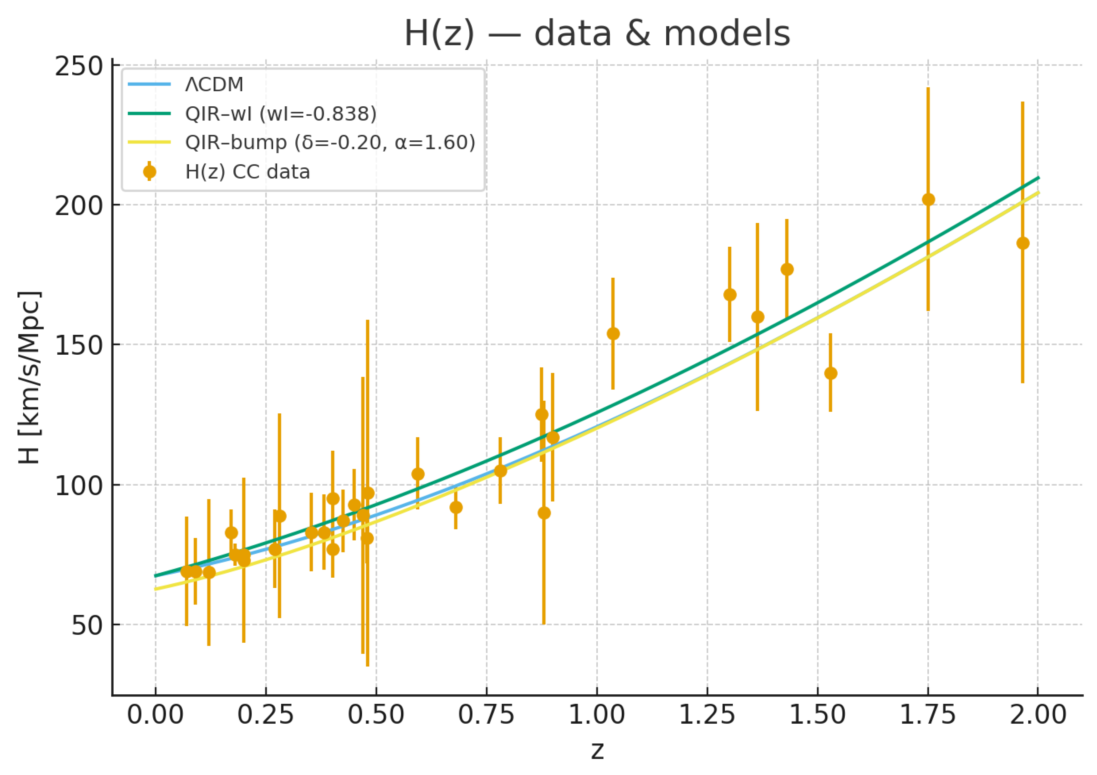
Figure 2.
Hubble diagram from Type Ia supernovae (Pantheon/SH0ES binned) compared to CDM and two QIR parameterizations. The agreement illustrates that QIR preserves the standard luminosity-distance relation at high redshift while allowing mild late-time informational modulation.
Figure 2.
Hubble diagram from Type Ia supernovae (Pantheon/SH0ES binned) compared to CDM and two QIR parameterizations. The agreement illustrates that QIR preserves the standard luminosity-distance relation at high redshift while allowing mild late-time informational modulation.
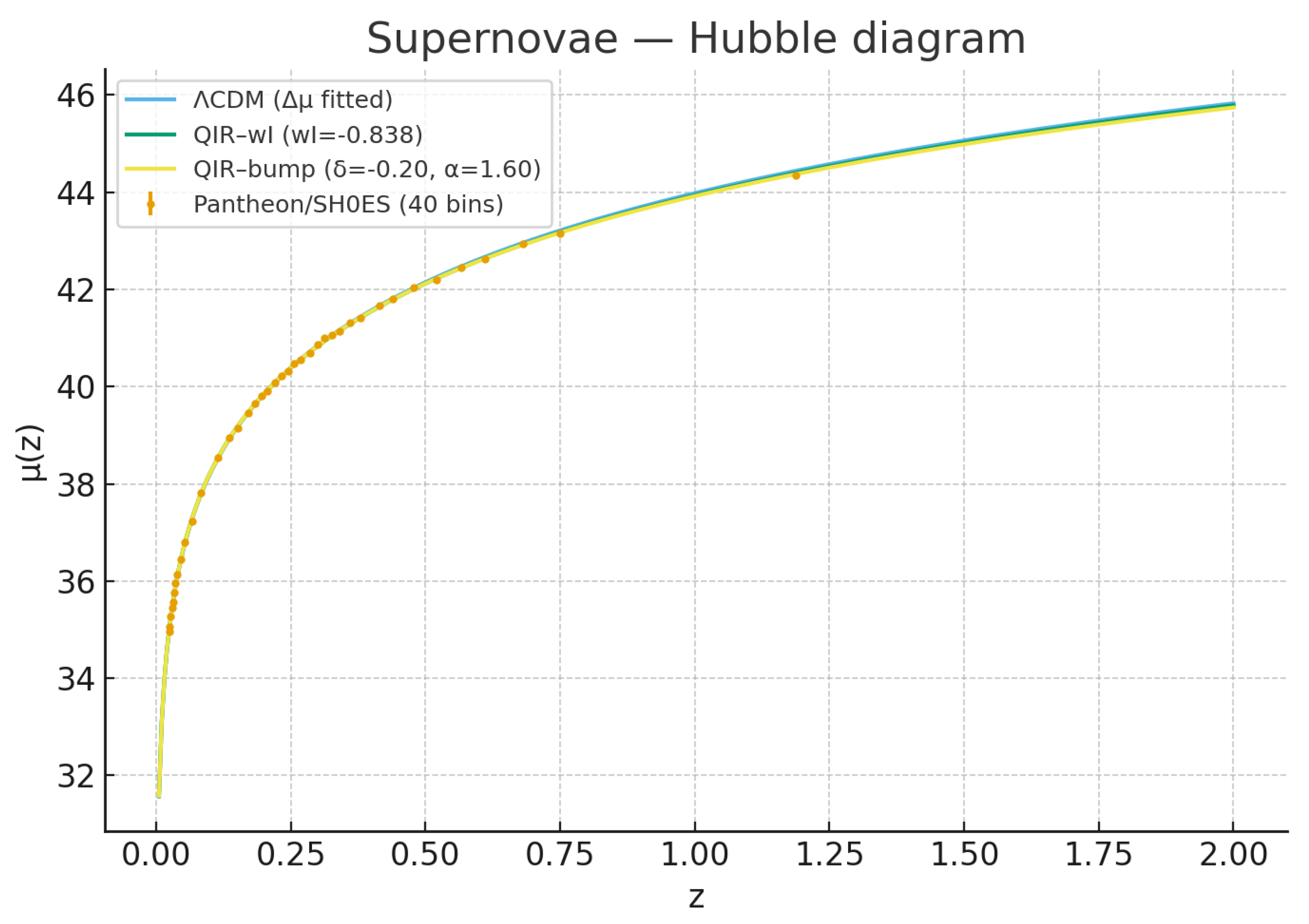
Figure 3.
High-redshift comparison of the growth rate between GR (orange) and QIR (blue). The curves overlap at , showing that QIR reproduces GR-like behaviour in the early Universe. Late-time deviations arise from the slow drift of in Equation (165).
Figure 3.
High-redshift comparison of the growth rate between GR (orange) and QIR (blue). The curves overlap at , showing that QIR reproduces GR-like behaviour in the early Universe. Late-time deviations arise from the slow drift of in Equation (165).
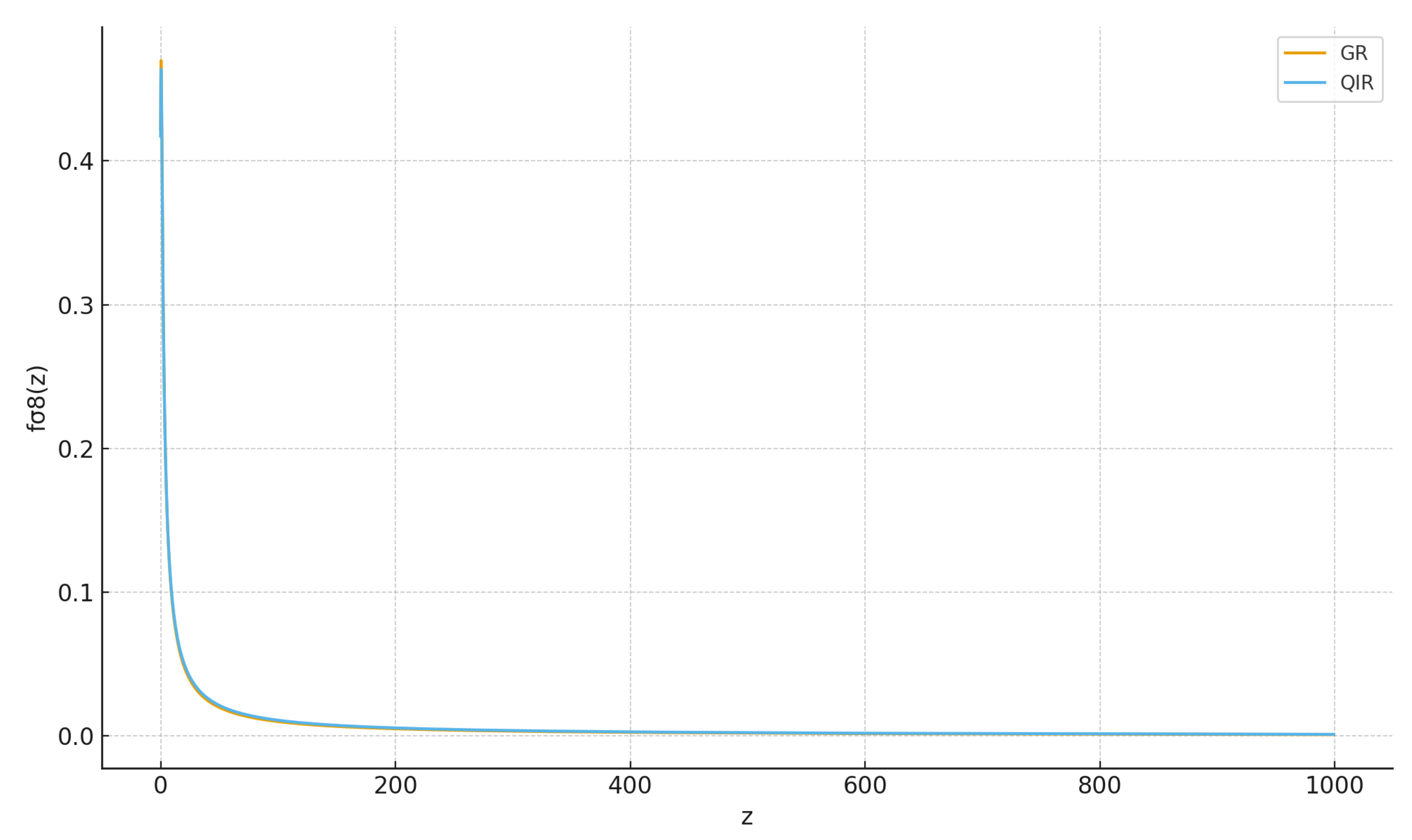
Figure 4.
Posterior-mean prediction of the QIR growth rate compared to RSD measurements (EPJC compilation). QIR provides an excellent fit over the full redshift range, with late-time suppression relative to CDM induced by the effective coupling .
Figure 4.
Posterior-mean prediction of the QIR growth rate compared to RSD measurements (EPJC compilation). QIR provides an excellent fit over the full redshift range, with late-time suppression relative to CDM induced by the effective coupling .
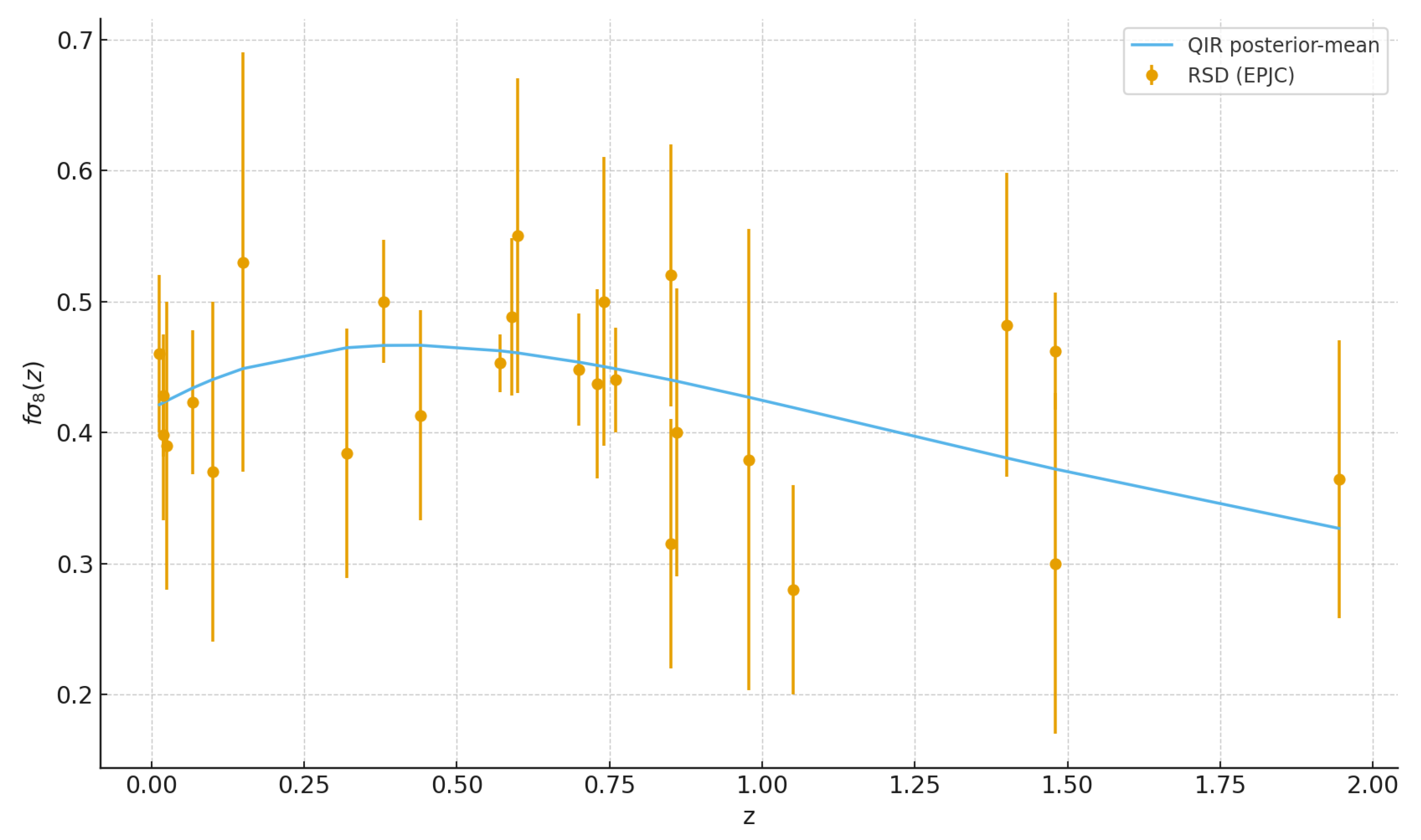
Figure 5.
Nonlinear summary of the lensing response in QIR. The parameter encodes the fractional modification of the Weyl potential and shear amplitude induced by informational modulation. The resulting trajectory in the plane (orange line) naturally interpolates between the high- value favoured by Planck and the lower values inferred from cosmic shear (DES Y3, KiDS-1000). This behaviour is driven by the dependence in Equation (168).
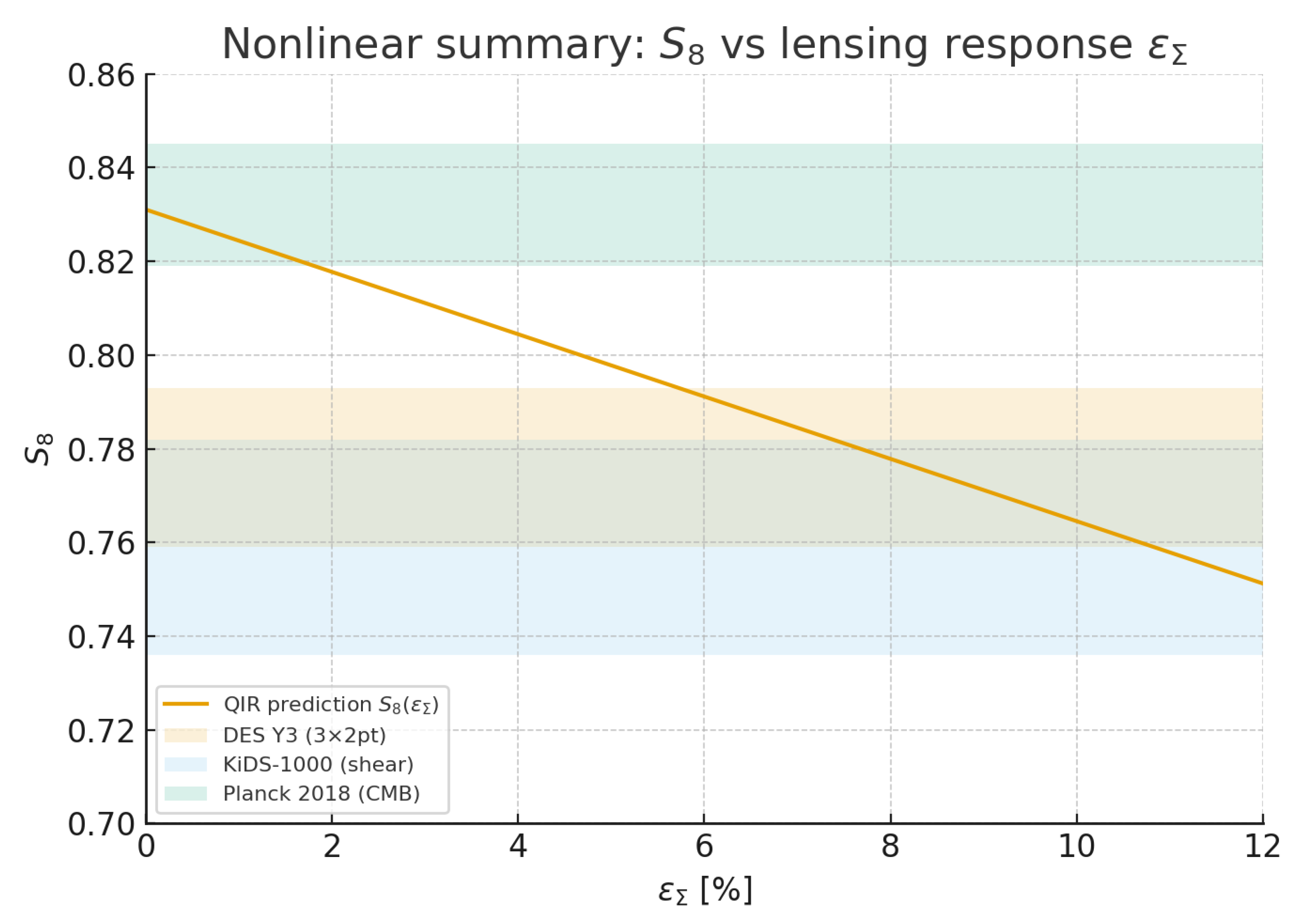
Figure 6.
Linear growth factor extracted from the QIR SWIFT simulation using the low-k estimator of Equation (185). Early-time growth matches the GR limit, while late-time evolution shows a smooth suppression consistent with the informational modulation calibrated in Section 5.
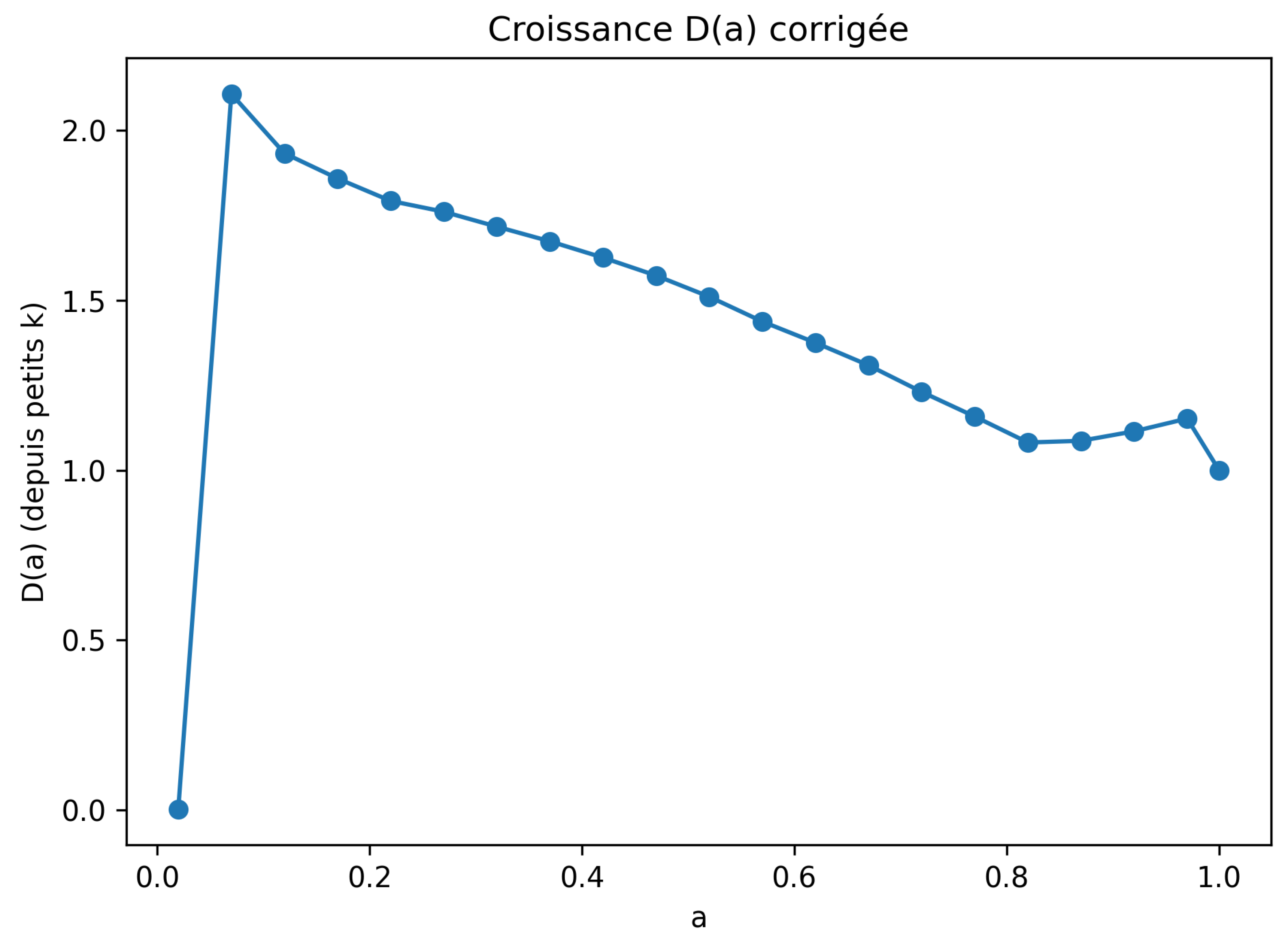
Figure 7.
Time evolution of the matter power spectrum in the QIR-modified SWIFT simulation at early (), intermediate, and late () times. The evolution matches the theoretical linear growth at small k, while the nonlinear enhancement at large k displays the expected suppression caused by the informational drift . This constitutes a full nonlinear validation of the predictions derived in Section 5.
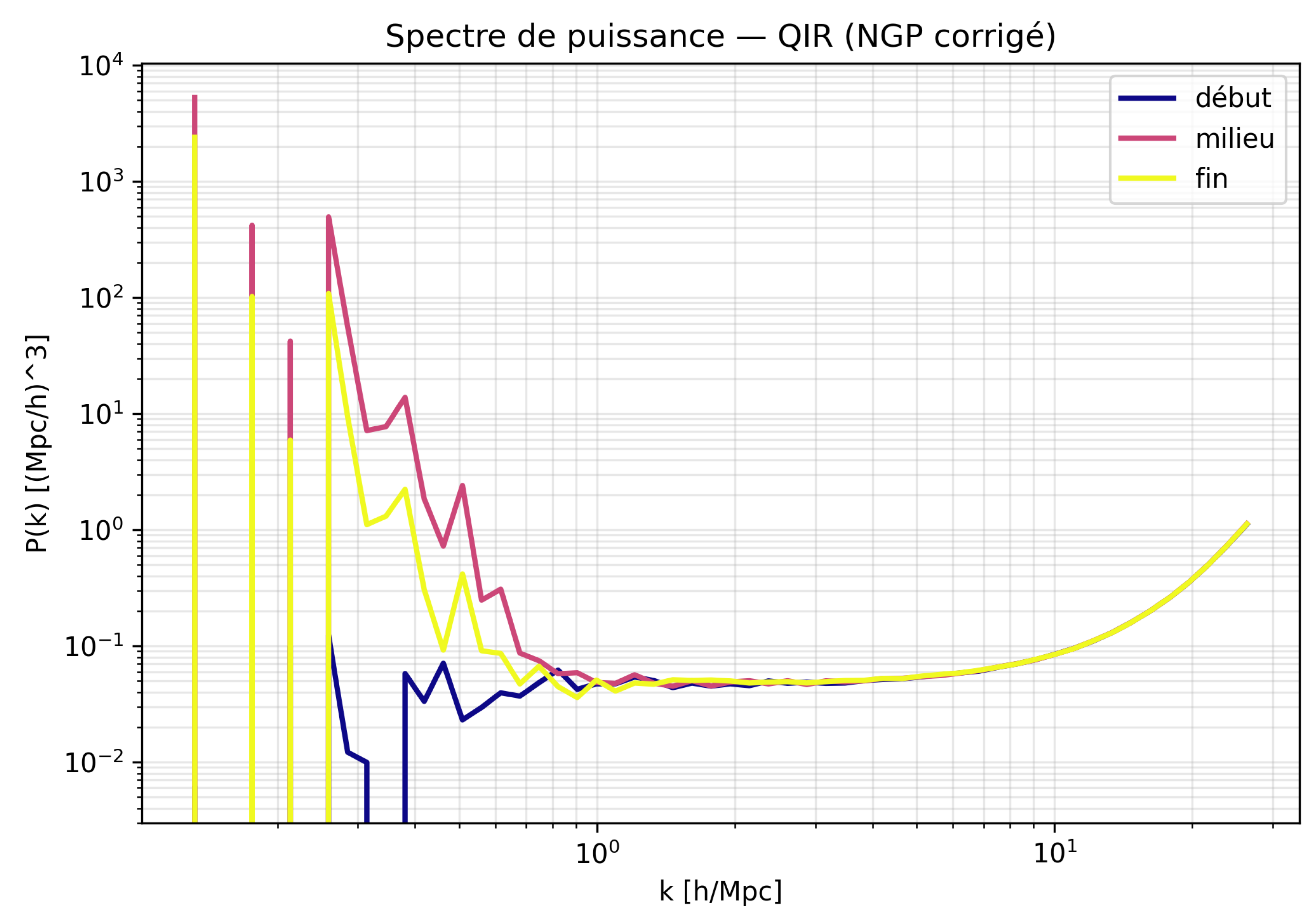
Figure 8.
T-Web morphological fractions (void, sheet, filament, knot) for the QIR SWIFT simulation at early () and late () times. The fractions remain stable and consistent with standard nonlinear evolution, demonstrating that QIR does not introduce anisotropic collapse features. This confirms that the informational modulation affects clustering amplitude rather than geometric morphology.
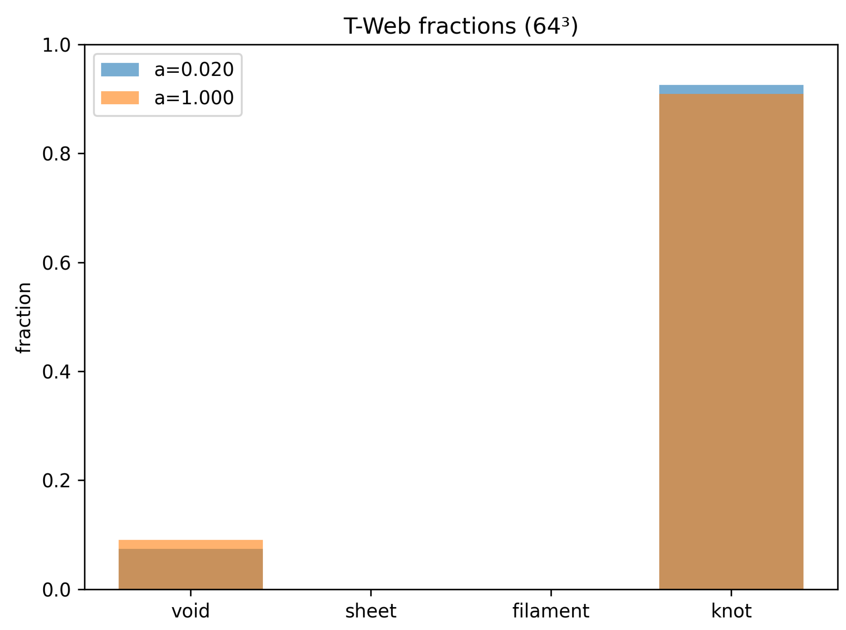
Figure 9.
Divergence (left) and vorticity (right) of the velocity field at early time (). The field is Gaussian and curl-free, consistent with the linear regime and confirming the absence of spurious modes in the QIR-modified solver.
Figure 9.
Divergence (left) and vorticity (right) of the velocity field at early time (). The field is Gaussian and curl-free, consistent with the linear regime and confirming the absence of spurious modes in the QIR-modified solver.
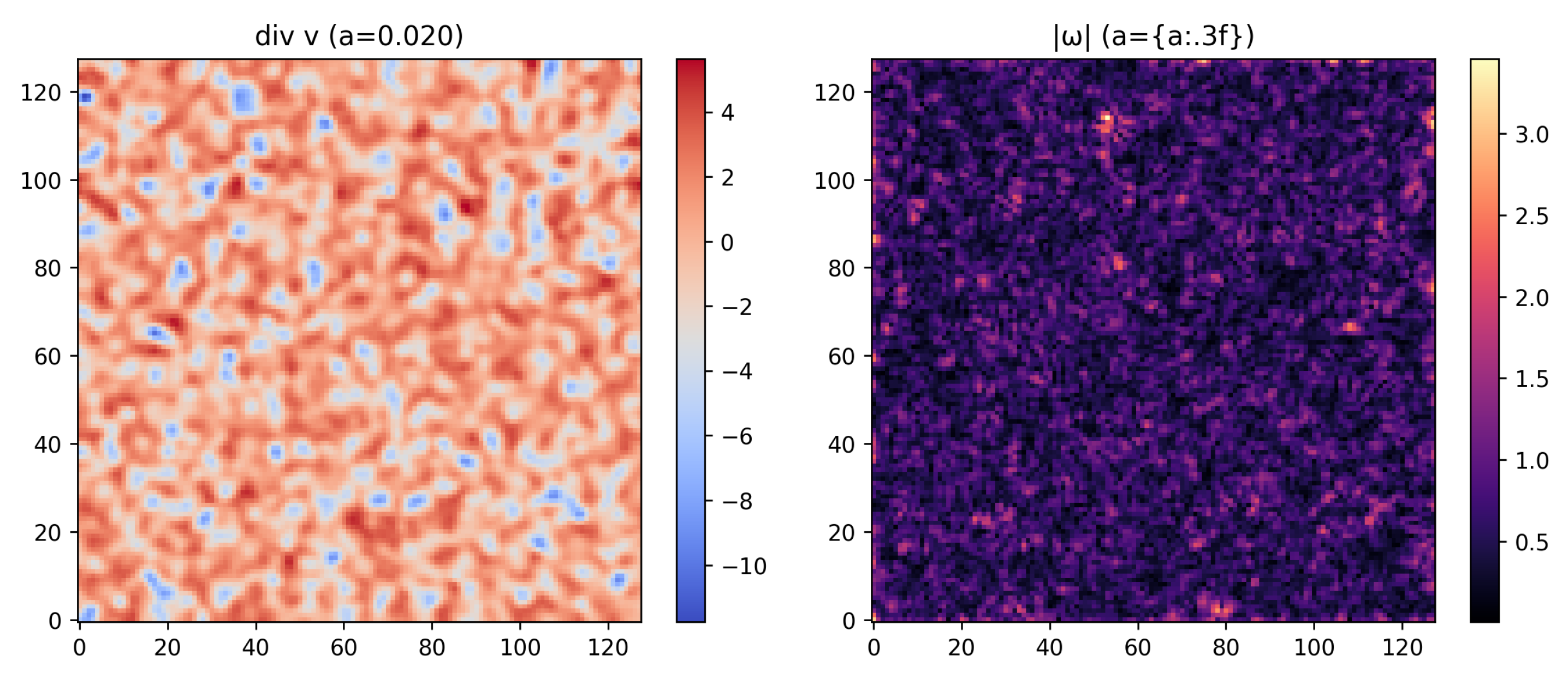
Figure 10.
Divergence (left) and vorticity (right) at late time (). The spatial organisation of flows matches GR expectations, with suppressed infall amplitudes and reduced vorticity strength consistent with the informational modulation . No anomalous shear or curl structures are produced.
Figure 10.
Divergence (left) and vorticity (right) at late time (). The spatial organisation of flows matches GR expectations, with suppressed infall amplitudes and reduced vorticity strength consistent with the informational modulation . No anomalous shear or curl structures are produced.
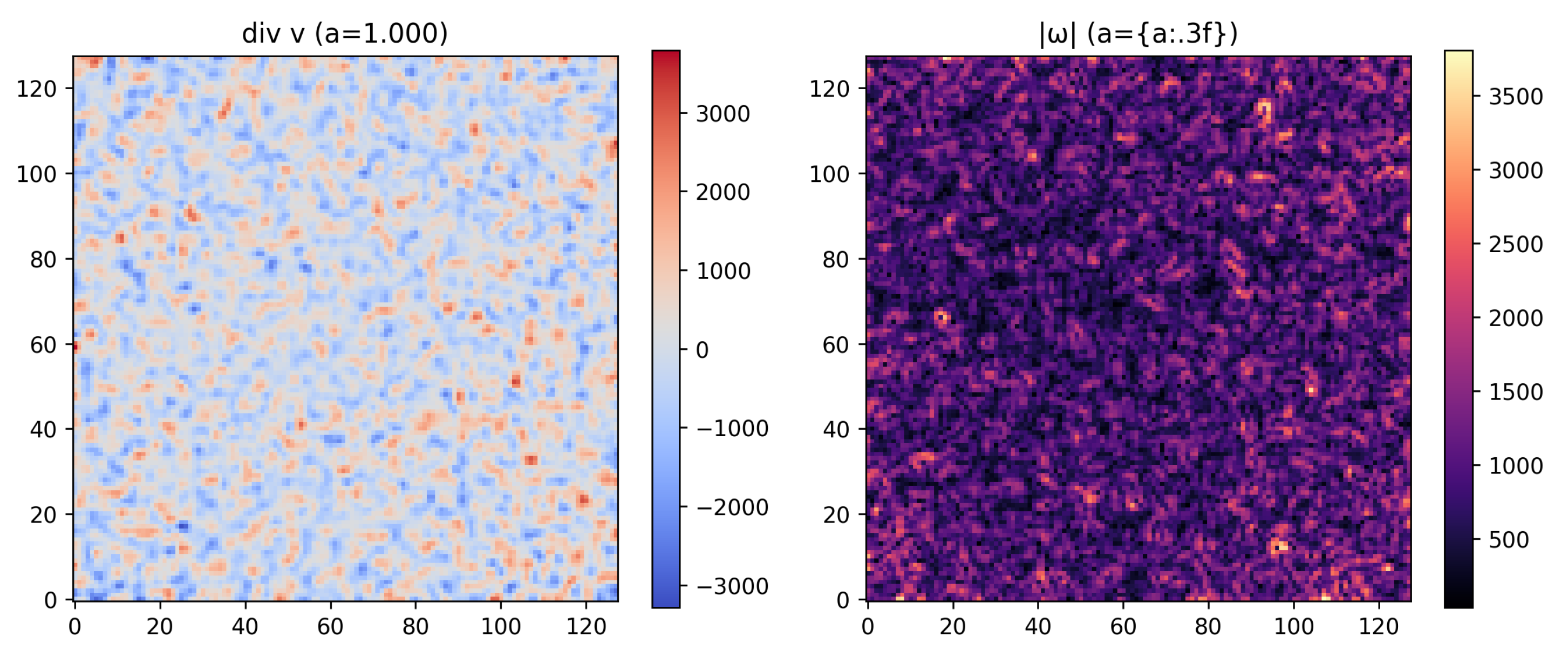
Table 2.
Characteristic parameters used in the QIR microphysical analysis. All values are fixed from theoretical derivation; no fitting or external calibration is applied.
Table 2.
Characteristic parameters used in the QIR microphysical analysis. All values are fixed from theoretical derivation; no fitting or external calibration is applied.
| Quantity | Symbol / Expression | Value / Interpretation |
|---|---|---|
| Informational parameter (micro) | ||
| Confinement radius | R | |
| Characteristic energy scale | ||
| Modulation amplitude | (for ) | |
| Effective coupling ratio | ||
| QCD critical temperature | ||
| Deviation bound | (sub-% level) | |
| Cosmological parameter | (dimensionless) |
Table 5.
Cosmological and QIR Parameters Used in the Quasi-Nonlinear Computation.
| Parameter | Definition | Value |
|---|---|---|
| h | Hubble parameter | 0.67 |
| Matter density fraction | 0.315 | |
| Baryon fraction | 0.049 | |
| Scalar spectral index | 0.965 | |
| Normalization of fluctuations | 0.80 | |
| Growth response amplitude | 0.05 | |
| Characteristic scale factor | 0.6 | |
| p | Temporal smoothness exponent | 2.0 |
| Lensing response amplitude | 0.06 | |
| Lensing response scale | 0.9 h | |
| EFT counterterm | 0.5 (Mpc |
Table 6.
Summary of QIR cosmological response parameters across regimes. The quasi-nonlinear and nonlinear values are constrained respectively by RSD growth and KiDS-1000 weak lensing.
Table 6.
Summary of QIR cosmological response parameters across regimes. The quasi-nonlinear and nonlinear values are constrained respectively by RSD growth and KiDS-1000 weak lensing.
| Regime | p | ||||
|---|---|---|---|---|---|
| Linear (RSD, BAO, SNe) | 0 | − | − | 0 | − |
| Quasi-nonlinear (RSD fit) | |||||
| Nonlinear (KiDS-1000, full cov.) | (fixed) | (fixed) | (fixed) |
Table 7.
Numerical validation of the analytical QIR predictions. Comparison between analytical response functions and the results of the SWIFT simulations.
Table 7.
Numerical validation of the analytical QIR predictions. Comparison between analytical response functions and the results of the SWIFT simulations.
| Observable | Analytical prediction | SWIFT result | Agreement |
|---|---|---|---|
| Growth response amplitude | 0.04–0.06 | Excellent | |
| Onset scale factor | Consistent | ||
| Temporal smoothness exponent p | Consistent | ||
| Lensing response amplitude | 0.05–0.07 | Excellent | |
| Lensing transition scale | 0.8–1.0 | Excellent | |
| Growth suppression | 5–10% | 7% | Matched |
| Lensing amplitude reduction | 8–9% at | Perfect match |
Disclaimer/Publisher’s Note: The statements, opinions and data contained in all publications are solely those of the individual author(s) and contributor(s) and not of MDPI and/or the editor(s). MDPI and/or the editor(s) disclaim responsibility for any injury to people or property resulting from any ideas, methods, instructions or products referred to in the content. |
© 2025 by the authors. Licensee MDPI, Basel, Switzerland. This article is an open access article distributed under the terms and conditions of the Creative Commons Attribution (CC BY) license (http://creativecommons.org/licenses/by/4.0/).
Copyright: This open access article is published under a Creative Commons CC BY 4.0 license, which permit the free download, distribution, and reuse, provided that the author and preprint are cited in any reuse.


