1. Introduction
Bibliometric analyses reveal a growing interest in the study of forest ecosystems, likely reflecting the increasing challenges they face [
1]. Indeed, on the one hand, forests provide a wide range of ecosystem services, including food production, timber and fuel supply, water conservation and regulation, carbon sequestration, biodiversity protection, climate regulation, as well as ecotourism and other recreation activities [
2]. However, one the other hand, their long-term sustainability is increasingly threatened by multiple anthropogenic pressures, particularly the expansion of agricultural lands and urban areas, along with the adverse impacts of climate change (CC) [
3]. CC, in turn, manifests through prolonged droughts, disruptions in water availability, soil erosion, and declining soil fertility - factors that collectively weaken forest ecosystems, reduce their capacity to withstand and recover from such perturbations [
3,
4] and ultimately increases global tree mortality [
5]. A combination of interacting factors is at play; for instance, the more frequent droughts observed over the past decade have not only caused water shortages and induced physiological stress in trees, but have also triggered indirect damage through pest outbreaks - most notably bark beetle infestations [
6]- and increased the risk of large-scale fires [
7].
Water is a key component to understand ecosystem functioning. Its circulation and the complex interactions within the soil–tree–atmosphere continuum are central concerns in ecohydrology. While climate and soil moisture regulate vegetation dynamics, forest ecosystems also strongly influence the overall water balance and generate multiple feedback loops [
8]. Hence, soil moisture and vapor pressure deficit appear among the most influential factors controlling forest water use [
9].
Characterizing the spatial and temporal dynamics of soil water storage is therefore essential. This need has, for instance, motivated the development of large-scale soil moisture monitoring databases [
10] and efficient treatment of satellite-based measurements [
11]. Ground-based observation networks, focusing on the critical zone and supporting interdisciplinary research, continue to play a crucial role in the development and validation of such approaches [
12,
13]. Moreover, many studies—particularly those with predictive objectives related to water resources under CC - rely on models in which hydrodynamic properties must be accurately defined [
14,
15]. With advances in computational material and methods, subsurface and groundwater flows are now widely represented in hydrological models using the Richards’ equation, particularly when applied at the catchment scale [
14,
15,
16,
17]. The hydrodynamic parameters used to describe the water retention and hydraulic conductivity curves of porous media can be estimated through pedotransfer functions, which are generally derived from particle-size analyses of soil samples [
14,
18,
19]. Other approaches based on geophysical measurements can also be considered to characterize subsurface structures and properties in a less intrusive manner and/or to cover a larger spatial extent [
20,
21]. When soil moisture or drainage data are recorded in situ (e.g., TDR sensors and/or lysimeters), it becomes possible to relate hydrodynamic parameters to time series through an inverse modeling approach. Although such methods require numerical expertise and measurement efforts that can be complex due to field constraints, they nevertheless yield valuable and insightful results [
19,
22]. The presence of rock fragments in the soil is often neglected, as most hydrodynamic models are not designed to represent their influence. Nevertheless, introducing appropriate corrections may be essential to accurately evaluate water dynamics and storage in porous media [
23,
24].
A study conducted at the Strengbach catchment Observatory (Vosges Mountains, France) investigated the impact of monitoring frequency on the estimation of soil hydrodynamic parameters and proposed a consistent parameter set derived from matric potential measurements along a vertical soil profile [
22]. Following severe forest dieback, largely attributed to pest outbreaks, the spruce stand at this site was completely clear-cut, and new monitoring systems were installed in 2022 on two more resilient plots.
The primary objective of the present study is to propose sets of hydrodynamic parameters suitable for hydrological modeling within the forested Strengbach catchment. These parameters are derived for two long-term monitoring plots, respectively dominated by spruce (Picea abies) and beech (Fagus sylvatica). The original results presented here are based on soil water content measurements obtained from two vertical profiles where soil samples were collected and analyzed. A dedicated methodology is described to refine the conventional approach based on PTFs by explicitly accounting for the influence of soil stoniness, thereby improving the representativeness of the derived hydrodynamic properties.
2. Materials and Methods
The following sections successively present the study site and the characteritics of the two plots studied. The instruments used for data acquisition are then described, along with the models employed to derive the hydrodynamic parameters. In sequence, the calculation of potential evapotranspiration and its implementation in the BILHYDAY model contribute to the estimation of actual evapotranspiration (AET). This variable is involved in defining the upper boundary condition used in the inverse modeling approach based on Richards’ equation, which is also presented. Finally, a specific section details the methodological aspects necessary to understand the steps involved in parameter estimation.
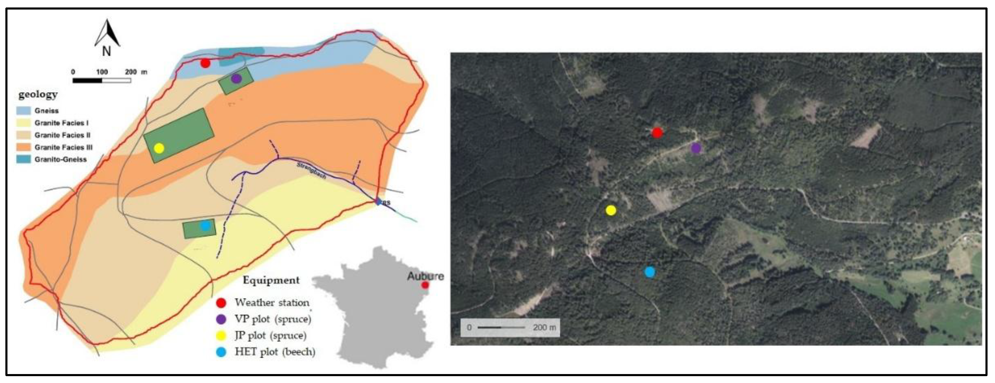
2.1. General Description of the Site
The Strengbach research catchment is located in the high-altitude commune of Aubure (Vosges Mountains, Haut-Rhin, France, see
Figure 1). This experimental site covers an area of 0.8 km² and extends from 850 to 1150 m a.s.l. Approximately 80% of the catchment is forested, with about 76% consisting of a monospecific Norway spruce (Picea abies) plantation and the remaining area dominated by beech (Fagus sylvatica) [
25]. From a pedological perspective, the catchment is characterized by acidic brown and ochreous podzolic soils developed on a calcium-poor granitic substrate [
25].
Meteorological, hydrological, and geochemical variables of the Strengbach catchment have been continuously monitored since 1986 by the Hydro-Geochemical Environmental Observatory (OHGE;
https://ohge.unistra.fr). The initial establishment of the monitoring network was motivated by research on acid rain and its effects on forest ecosystems. Current investigations now address a wider range of environmental issues, including forest decline associated with nutrient-poor soils [
26,
27], the impacts of climate change [
28], and water resource management [
29,
30]. In addition, methodological developments are being pursued to improve the characterization of subsurface aquifers throughout multidisciplinary research [
20,
25,
31].
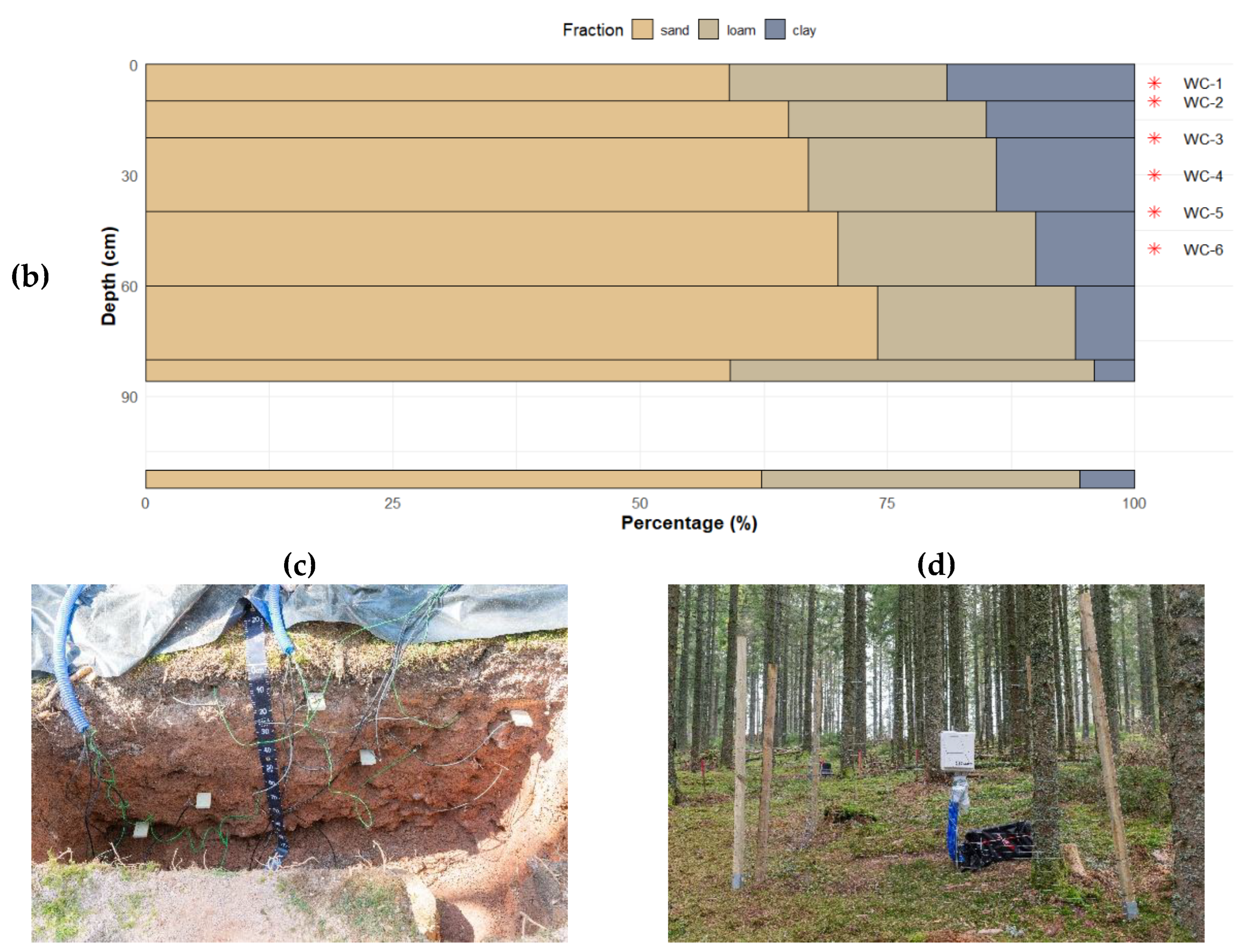
2.2. Monitoring Devices and Associated Measurements
The Strengbach catchment is equipped with a meteorological station located in an open area at the top of the mountain (cf.
Figure 1). Precipitation is measured using a tipping-bucket rain gauge (Précis Mécanique, model R5-302 b). Air temperature and relative humidity are recorded at a height of 1.5 m with a Vaisala HMP45C probe. Wind speed and direction are measured with an R.M. Young anemometer (model 05103), and incoming global radiation is monitored using a Kipp & Zonen pyranometer (model CM6B). All measurements are recorded by a Campbell CR1000X datalogger at a 10-minute time step.
For soil moisture monitoring, in the spruce plot (denoted JP in
Figure 1), a soil pit was excavated to install Campbell TDR probes (model CS616) at depths of 13, 31, 52, 72, and 92 cm. In addition, four Campbell temperature probes (model 107) were installed at the first four depths to enable temperature correction. The sensor raw period (τ
raw, in μs) is corrected using a quadratic function of soil temperature (T
soil, in °C) defined in equation 1:
Following several laboratory tests conducted on soil samples, the standard quadratic calibration equation provided by the manufacturer was retained to derive the volumetric water content (θ, in m³/m³), as shown in equation 2:
In the beech plot (denoted HET in
Figure 1), a 50-cm Campbell SoilVue10 probe was installed, providing measurements of volumetric water content at depths of 5, 10, 20, 30, 40, and 50 cm. This sensor internally applies the correction and calibration equations and directly reports the volumetric water content. For both plots, WC data were recorded every 10 minutes on Campbell CR1000 (JP) and CR1000X (HET) dataloggers.
Notice that the SoilVue10 sensor does not require excavation of a pit but only the drilling of a hole using an auger with a slightly smaller diameter than that of the probe, into which it is then inserted. Owing to the pedological characteristics of the stand, a certain period was necessary for proper soil–probe contact to be established. A preliminary data processing step was applied to filter out measurements affected by preferential flow along the vertical probe and by water accumulation at the bottom of the hole. It should also be noted that this device operates at shallower depths and does not rely on exactly the same type of sensors as the installation on JP stand.
Although these data are primarily used as input for the inverse modeling process, the precipitation and soil moisture time series will be presented in the Results section to enhance the comprehension and assessment of the modeling outcomes. A complementary hydrological analysis will also be provided.
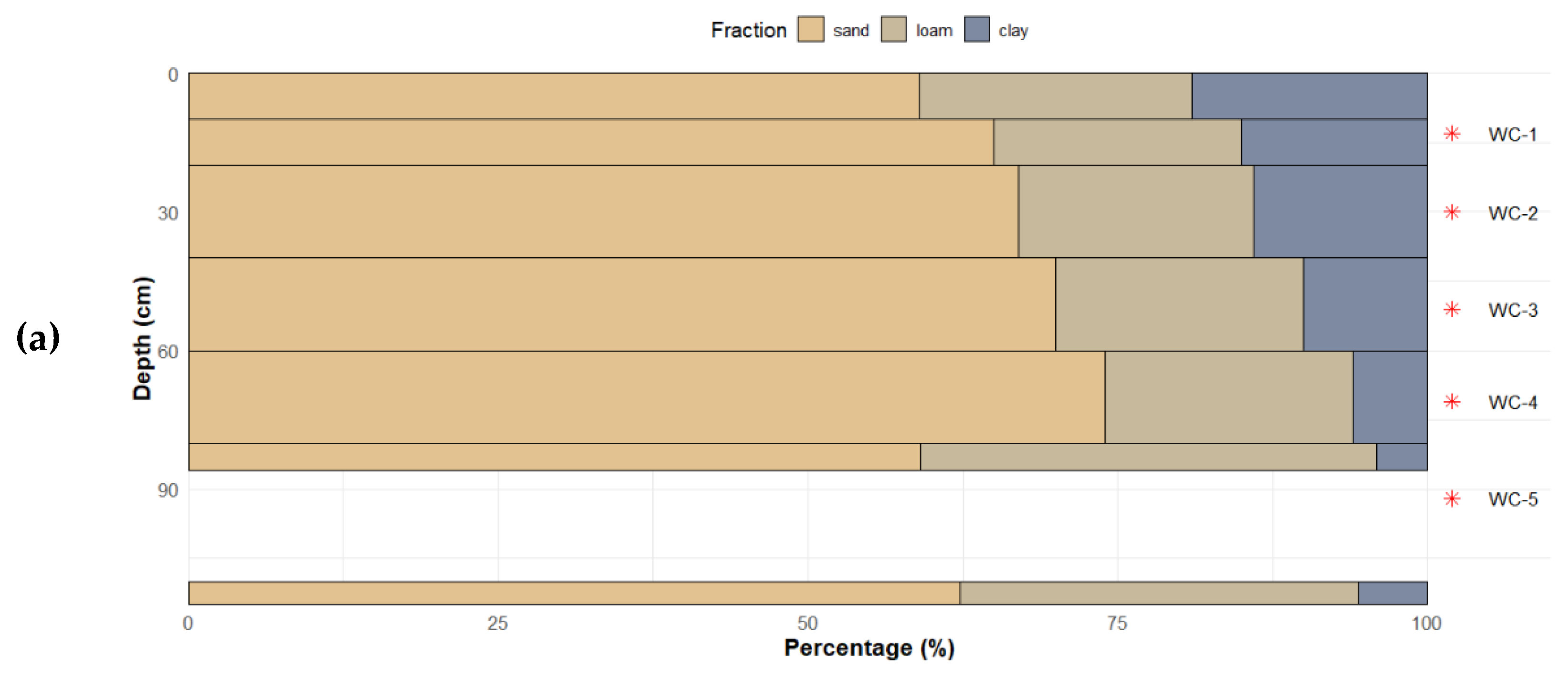
2.3. Vertical Profiles and Soil Properties
Undisturbed samples were collected in April 2022 from the JP plot at eleven depths (
Figure 2a). Soil composition was determined using a laser diffraction particle sizing technique. The soil was mainly composed of particles larger than 2 μm, corresponding to sand and loam fractions, with the latter generally more abundant, averaging 53% compared to 35% for the sand fraction. For the HET plot (
Figure 2b), data from [
26] were used. They are based on the same analytical technique and show that the sand fraction is dominant, exceeding 59% across the depths analyzed, with a mean value of 65%, compared to 24% and 11% for the loam and clay fractions, respectively.
Sensor locations are shown in
Figure 2a,b (red stars on the right side). Due to restrictions in operating the devices and the complexity of parameter estimation under natural conditions, the domain discretization was simplified. A step in our methodology described in section 2.5 will consist of selecting relatively homogeneous layers, each containing at least one sensor, and estimating their hydrodynamic parameters.
Figure 2c,d show the pit excavated for sensor installation and sampling, with visible coarse elements that were not captured by the soil sampling cylinders of approximately 4 cm radius. The site was refilled while maintaining the original sequence of soil layers as much as possible, in order to monitor moisture dynamics in an environment minimally disturbed given the chosen methodology.
2.4. Numerical Methods
2.4.1. Potential and Actual Evapotranspiration
The choice of the potential evapotranspiration (PET) estimation method is crucial for accurately quantifying water fluxes in hydrological models [
32]. To ensure consistency with previous studies conducted in the Strengbach watershed [
22,
33], the formulation derived from the Penman equation by Brochet and Gerbier [
34] was adopted, as presented in Equation (3). Earlier studies have demonstrated that this approach accounts for the specific characteristics of the experimental site, particularly in the computation of net radiation in the radiative term (first component on the r.-h. s. term of Equation (3)) and in the formulation of the advective term (second component on r.-h. s. term of Equation (3)).
PET
BG is given in mm.d
-1, Δ is the derivative of saturated vapor pressure versus temperature (mbar.K
-1) expressed as the air temperature Ta (°C) (see Equation (4)), R
n is the net radiation at the canopy surface (cal.cm
-2.d
-1), δ
e is the saturation vapor pressure deficit (mbar) expressed at the air temperature T
a (°C) and the relative humidity H
r (%) see Equation (5)), γ is the psychrometric constant (0.66 mbar.K
-1) and u
10 is the adjusted wind speed at 10 m height (m.s
-1).
Originally, the estimation of net radiation was derived from measurements of global radiation, complemented by a sunshine duration table used for potential corrections. Consequently, the preceding equations (Equations (3)–(5)) enabled the calculation of the daily PETBG. Nevertheless, since meteorological measurements are available at higher frequency, PET can also be estimated at an hourly resolution (notice that daily and hourly values have been used in this study).
If PET represents the maximum evapotranspiration under well-watered conditions, the actual evapotranspiration (AET) accounts for water stress as well as precipitation intercepted and subsequently evaporated by vegetation foliage throughout the different seasons. An in-house code, BILHYDAY, based on a daily water mass balance and following a conceptual approach (see principles in [
35]), was used to estimate AET according to Equation (6):
where Tr refers to transpiration by the canopy (mm.d
-1), In is the interception (mm.d
-1) and SEvap is the soil and understored evaporation (mm.d
-1).
Meteorological variables such as wind velocity, net radiation, air temperature, relative humidity, and recorded precipitation are provided to BILHYDAY as input data, along with site-specific parameters describing the canopy, plant interception, soil evaporation, and ecophysiological characteristics. PET
BG is then computed, and the three components of AET in Equation (6) are partly driven by the maximum leaf area index (LAI), a dimensionless variable that characterizes plant canopies and is defined as the projected leaf area per unit ground area. Since runoff has never been observed at the experimental site due to the continuous vegetation cover, the BILHYDAY model is well suited for estimating AET on a daily time step and has been previously calibrated on different plots of our research catchment [
33,
36]. The AET time series used to define the upper boundary condition will be described in the results section.
2.4.2. Vadose Zone Model
The adopted hydrological model is based on Richards’ equation (Equation 7) [
37], which results from the combination of the mass conservation equation and the Darcy–Buckingham law, and describes water movement in a variably saturated porous medium.
where S is the storage coefficient (m
-1), θ is the volumetric water content (m
3.m
-3), θ
s is the saturated water content (m
3.m
-3), h is the pressure head (m), z is the vertical distance positive downward (m), t is the time (d) and K is the hydraulic conductivity (m.d
-1).
In addition, the standard Mualem–van Genuchten (MvG) model (Equations 8 and 9) [
38,
39] defines the relationships between negative pressure head, water content, and relative hydraulic conductivity (K
r, m.d
-1).
where S
e is the effective saturation (-), θ
r is the residual water content (m
3.m
-3), α is a parameter related to the mean pore size (m
-1), n is a parameter reflecting the uniformity of the pore size distribution (-), m = 1 – 1 / n is a parameter (-) [
39], K
sat is the saturated hydraulic conductivity (m.d
-1) and L is a parameter related to the tortuosity chosen here equal to 0.5 (-) [
38]. Notice that for saturated conditions (i.e. h ≥ 0), K = K
sat and S
e = 1.
The vertical profiles of forest soils contain a non-negligible proportion of stones and coarse fragments, which are generally not represented in undisturbed samples collected with cylinders and analyzed in the laboratory. To account for their effect on the evaluation of flow in the vadose zone, a corrective model for water content and hydraulic conductivity was implemented [
23]. This model consists of two equations (10) and (11) for the water content and hydraulic conductivity respectively [
23,
24,
40,
41].
In equations (10) and (11), the subscript b denotes the bulk value, whereas f refers to the fine soil fraction. The parameter a represents the hydraulic resistance of rock fragments to water flow and depends on their shape and size (-), while R
v denotes the relative volumetric fraction of stones (cm³.cm⁻³). The parameter a was set to 1.1 in accordance with [
41] while the coefficient R
v is adjusted according to the plot and soil layer in question.
Hence, a set of 5 parameters (Ksat, θs, θr, n, α) is needed for each layer of the considered domain. Finally, the model requires specification of upper and lower boundary conditions throughout the simulation period.
2.4.3. Simulations Achieved
Simulations for the period 2022–2025 were performed using WaMoS-IPE-1D (Water Movement in Soil – Inverse Parameter Estimation – 1D) respectively for the spruce and beach plots. The numerical methods implemented in this Fortran code to solve Richards’ equation (Equation 7) include: (i) a finite element method for spatial discretization; (ii) a fully implicit backward Euler scheme for temporal integration; (iii) a variable switching approach employing modified Picard or Newton methods for linearization [
42]; (iv) a heuristic time-stepping strategy based on iteration counts [
43]; (v) a switching, flux-controlled procedure for the top boundary condition to maintain physically realistic results [
44]; and (vi) a Levenberg–Marquardt iterative algorithm to solve the inverse problem [
45]. A detailed description of the code is provided in Lehmann and Ackerer [
46].
A uniform 1 cm mesh was adopted for the spatial discretization of both vertical profiles. Simulations were initialized with a specified hydrostatic pressure head profile derived from the lower water content measurement and allowed a sufficiently long warm-up period to ensure that initial conditions did not influence parameter estimation. An imposed flux boundary condition was applied at the soil surface, while the bottom boundary was defined as free drainage. As mentioned in section 2.4.1, the BILHYDAY code allows estimation of daily AET, which is then converted to hourly AET using equation (12). The top boundary condition is subsequently imposed at an hourly time step by subtracting the hourly AET to the rainfall.
2.5. Methodology Investigated for the Model Calibration
The proposed methodology consists in the following steps:
The first step consisted of subdividing the soil profile into homogeneous layers, each containing at least one sensor. Two different configurations to describe the 110 cm deep profile in the JP stand were set, while only one is used for the 100 cm deep HET profile.
- 2.
Initialization of hydrodynamic parameters
Field sampling and subsequent laboratory analyses enabled the determination of soil texture and composition for the different configurations described previously.
Table 1 presents the configurations for the JP and HET stands. Following [
22], initial estimates of the soil hydraulic parameters were obtained using the ROSETTA software based on PTFs [
18], which derives parameters from measured soil texture data.
- 3.
Adjustments to account stoniness
The granulometric analyses performed on undisturbed soil samples were considered representative of the fine soil fraction. In contrast, both simulated and measured water contents represent the global bulk soil response. Consequently, the initial hydraulic parameters were corrected using the volumetric stone fraction (R
v) reported in
Table 1 to account for the influence of stoniness on the soil water dynamics and the referring properties detailed in equations (10) and (11).
- 4.
Calibration and validation simulations
Given the available measurement ranges (which differ between the two sites), parameter inverse estimation was conducted using the WaMoS-IPE-1D model. The optimization procedure minimized an objective function defined as the mean squared error between observed and simulated water contents (θ
meas and θ
sim respectively):
where N
time is the number of observation times and N
sens denotes the number of layers instrumented with a sensor and used for the calibration.
Following [
22], the inverse modeling approach focused on optimizing three key parameters: the saturated hydraulic conductivity (K
s), the shape parameter (α), and the pore-size distribution index (n). Hence, on the one hand, applying equation (10) is really important to get a proper estimation of θ
r and θ
s that are not estimated by our inverse model. On the other hand, K
s will be optimized and equation (11) is only useful for initialization. The quality of the calibrated parameter set was subsequently assessed using the Kling-Gupta Efficiency criterion [
47] computed over the overall period of measurements according to equation (14):
where r refers to the correlation coefficient between simulated and observed WC, α to the ratio of their standard deviations, and β to the ratio of their mean values.
The Nash–Sutcliffe Efficiency (NSE) criterion [
48] given in equation (13) can also be computed:
where
refers to the mean volumetric water content of the i
th layer over the period of concern. KGE and NSE values approaching 1 reflect an excellent agreement between simulated and observed data, while negative values indicate that the model performs poorer than simply using the mean of the observations as a predictor.
Depending on the plot considered (with different data availability), four calibration periods were selected:
Calib.1: from 01 May 2022 to 30 September 2022 (no data available for HET),
Calib.2: from 01 April 2023 to 31 December 2023,
Calib.3: from 01 April 2024 to 31 December 2024,
Calib.4: from 01 October 2024 to 30 September 2025.
One objective of the calibration step is to investigate the impact of the period used for calibration on the estimation of the parameters. The rest of the period is used for validation step.
3. Results
This section is dedicated to (i) the presentation of the meteorological time series and to the estimation of the mean site-scale potential evapotranspiration (PET), (ii) the presentation of the results obtained for each plot (JP and HET respectively) regarding the imposed upper boundary conditions and the outcomes of the parameter estimation using the inverse modeling approach.
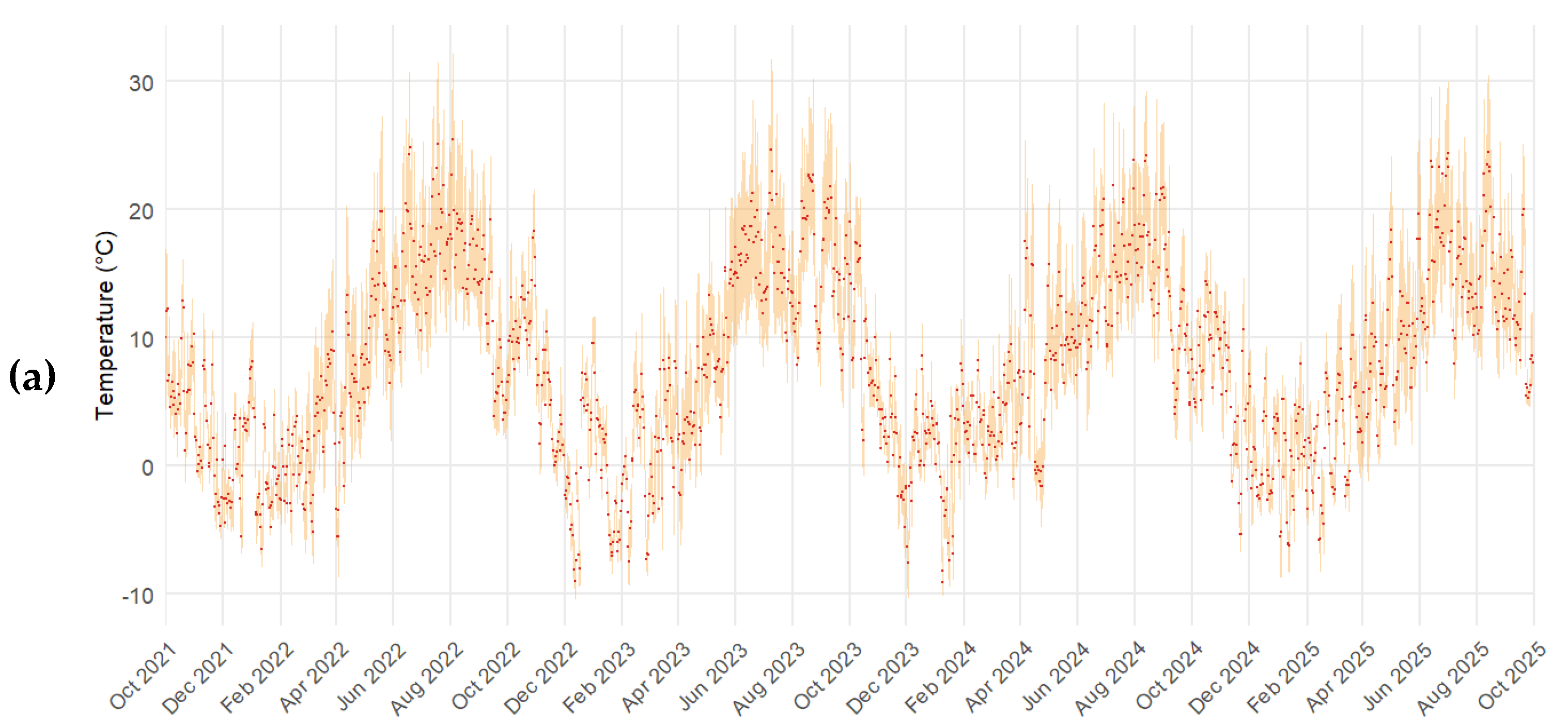
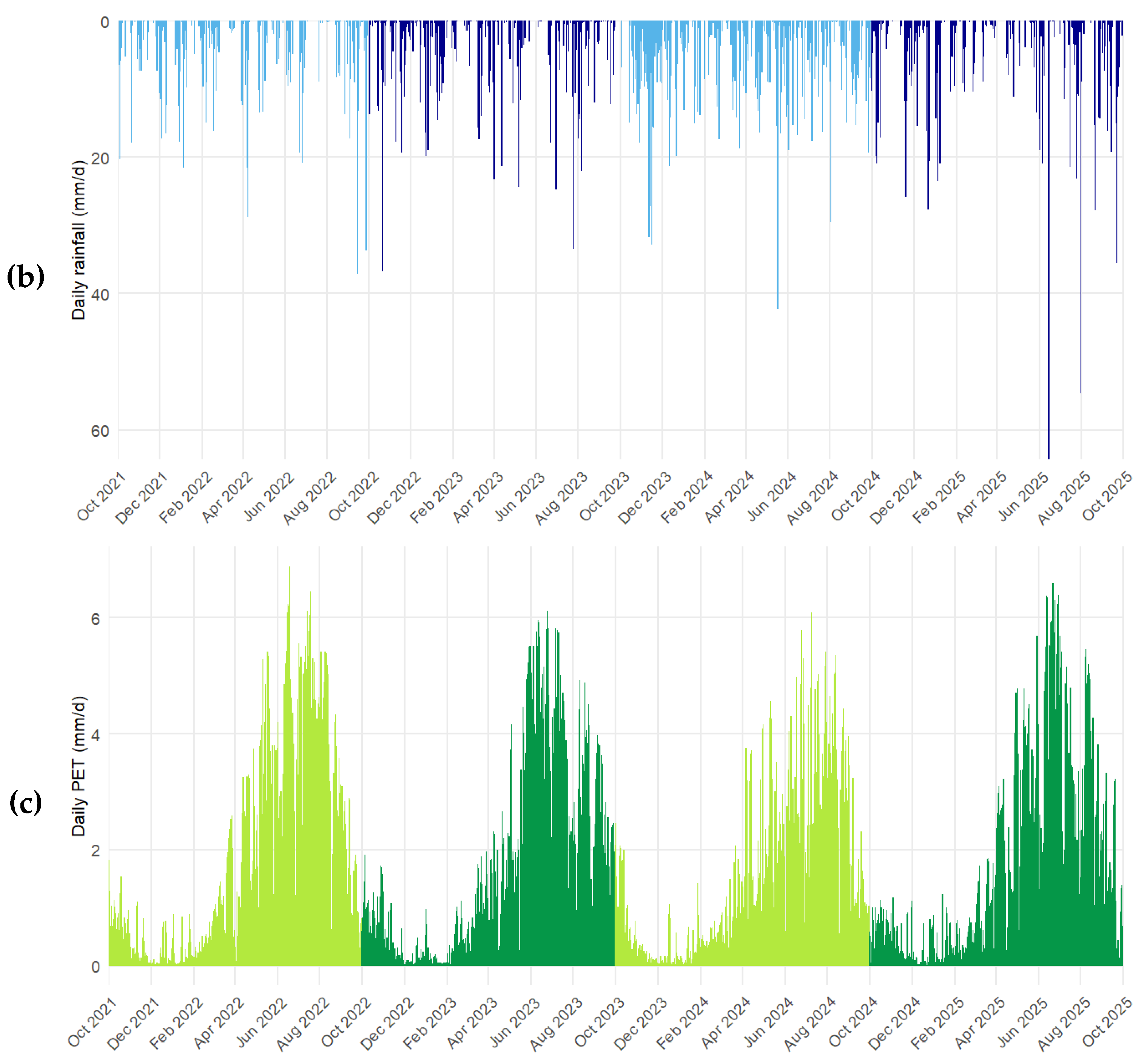
3.1. Time Series of Climatic Forcing and PET
Meteorological data for the period of interest are presented in
Figure 3. The hydrological year Y runs from October 1 of year Y to September 30 of year Y+1. Over the past 18 years, mean annual precipitation was 1223 mm, mean annual temperature 6.7°C, and total potential evapotranspiration (PET) 586 mm. The temporal evolution of daily precipitation and mean air temperature was used in the model described in section 2.4.1 to estimate potential evapotranspiration (PET). The four hydrological years considered exhibit substantial inter-annual variability relative to the 18-year climatological mean. The 2021 hydrological year, characterized by the summer drought of 2022, was the driest of the past 18 years (−20.7% rainfall, +18.8% PET relative to the long-term average), whereas 2023 was the wettest (+32% rainfall, -3.3% PET relative to the long-term average).
Figures S1 and S2 illustrate this meteorological variability.
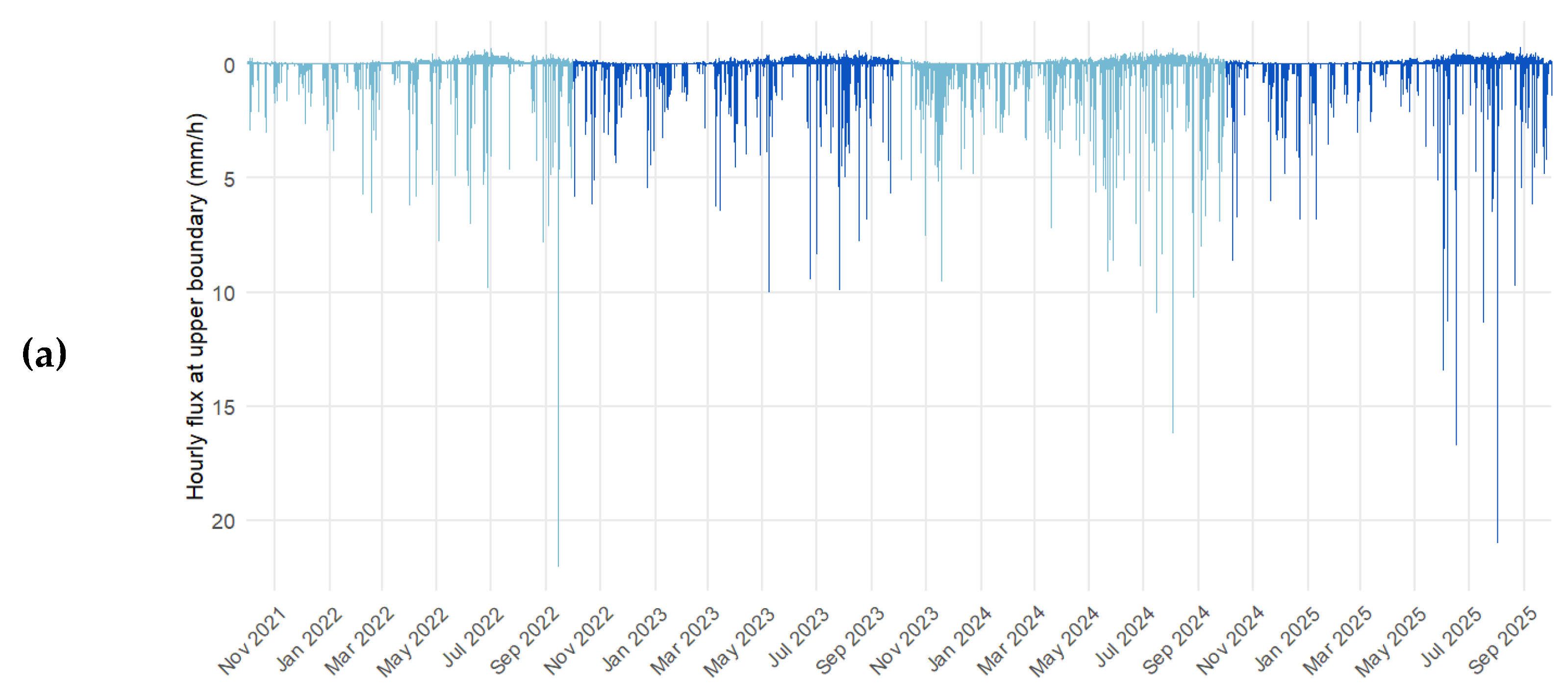
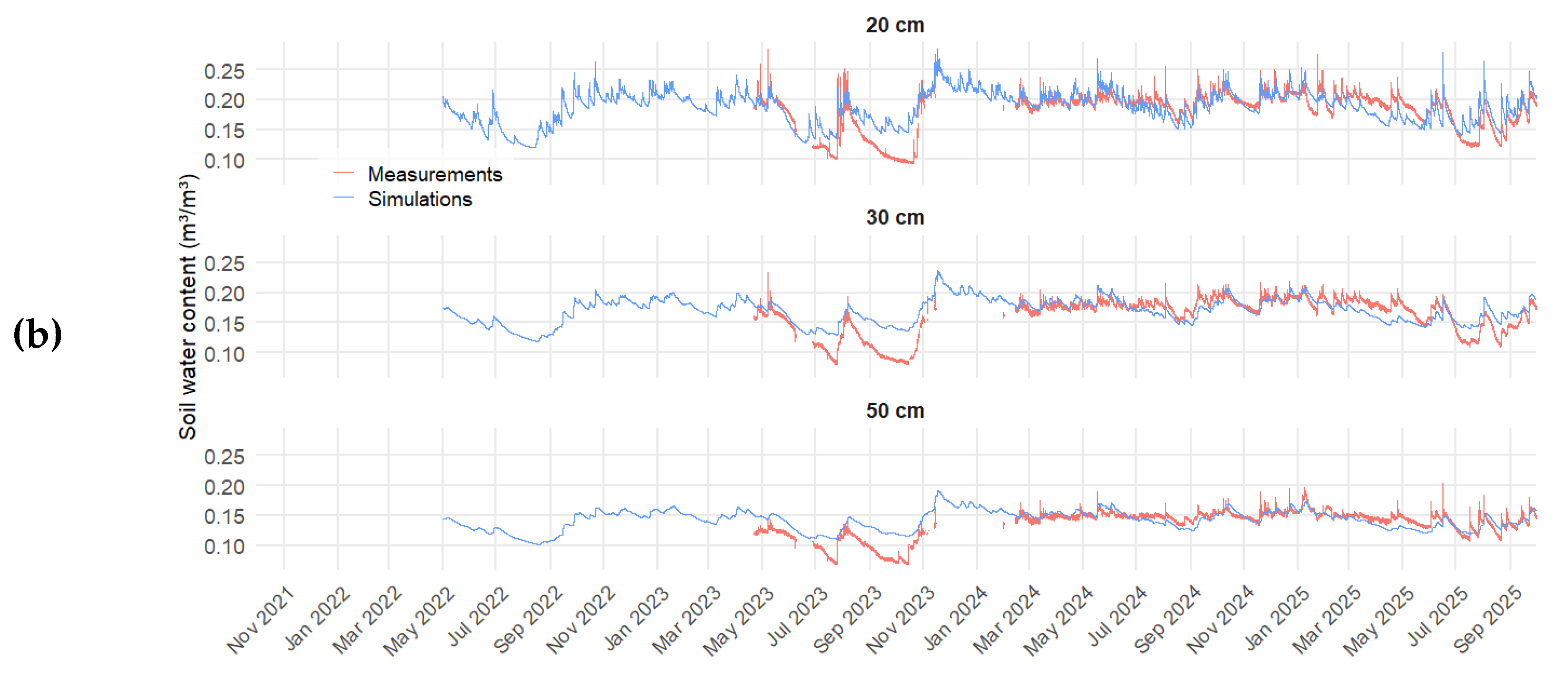
3.2. Results at JP Plot
Equation (11) was used to compute the AET at an hourly time step (based on BILHYDAY outputs). The resulting flux, used as a BC at the soil surface in the Wamos-IPE-1D model, corresponds to the difference between incoming precipitation and AET, as shown in
Figure 4a. As commonly observed, the flux is positive, indicating a net meteoric water input to the soil. However, at the seasonal scale, the situation is more contrasted: AET accounts for between 44% and 86% (for the 2023 and 2024 hydrological years, respectively) of precipitation during the spring season (April–June), and between 57% and nearly 75% (for the 2023 and 2022 hydrological years, respectively) of precipitation during summer (July–September).
Accordingly, the temporal evolution of soil WC was analyzed at depths of 31, 52, and 72 cm, as illustrated in
Figure 4b. This figure shows that the years 2022 and 2023 experienced marked and prolonged soil drying episodes, whereas in 2025, several rainfall events in August contributed to soil moisture recharge.
Equation (8) is applied to the parameters provided in
Table 2, derived from ROSETTA, in order to obtain θ
r and θ
s values adjusted to the stoniness level of the soil profile. Then, the Levenberg–Marquardt algorithm implemented in WaMoS-IPE-1D is run to optimize the three parameters
Ksat, α, and n.
Table 3 summarizes the best set of parameters obtained for each layer, noting that our investigations led us to retain discretization JP2 and calibration period no. 3.
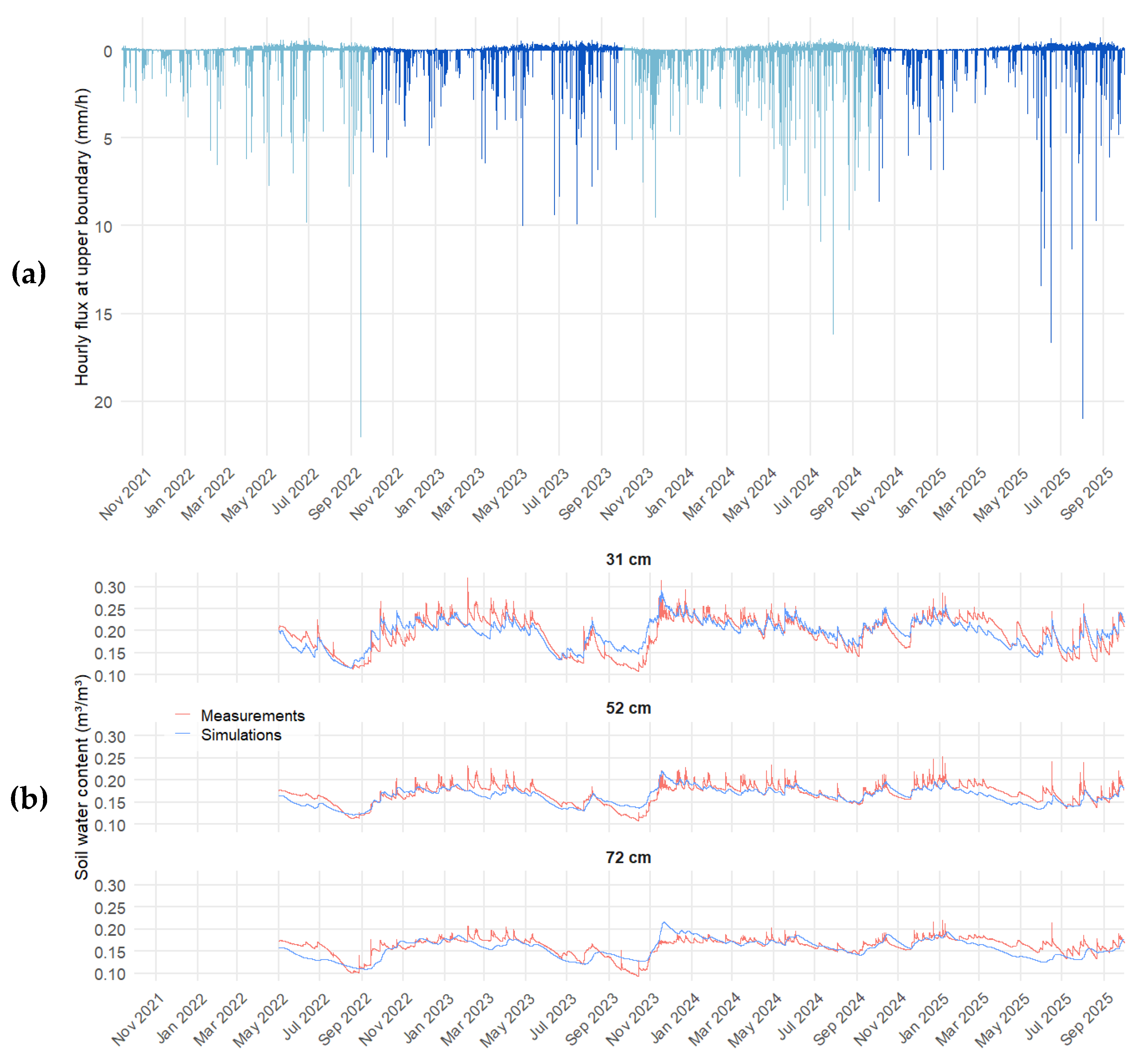
3.3. Results at HET Plot
Figure 5 a,b show the temporal evolution of the surface flux and of the soil WC at three depths (20, 30, and 50 cm) for the beech plot (HET). The descriptions are broadly similar to those provided for the spruce plot (JP). It is worth noting that sensor data could be reliably exploited starting from May 2023, although a few interruptions occurred thereafter. For this HET plot, the proportion of AET is approximately 10% lower than that observed for the spruce plot during spring, while the relative contribution during summer is slightly higher. The soil WC curves indicate that the spring and summer of 2023 (calendar year) correspond to the most pronounced soil drying period while the spring and summer of 2024 (calendar year) are the wettest recorded.
Following the same procedure as for the JP plot, the results obtained for the HET stand are presented in
Table 4. The best set of parameters corresponds to calibration period no. 4.
4. Discussion
As highlighted in [
22], the methodology focuses on optimizing three key parameters. To reduce the degrees of freedom of the inverse problem, the residual and saturated water contents are assigned fixed values. This approach is commonly applied in laboratory studies [
49,
50], whereas calibration using field data remains relatively scarce and requires additional supporting information [
51].
Identifying parameter sets that are simultaneously optimal at both the global scale profile and for each individual layer is challenging, due to potential compensatory effects among flow processes in the different layers and, possibly, equifinality issues. Furthermore, the performance metrics are not always consistent across criteria. All results are provided in the supplementary information (Section 2 for the parameters and section 3 for the efficiency criterion). The optimal configuration retained for the JP plot (i.e., JP2-3) was obtained from calibration during period 3; except for layer 2, the efficiency indices are higher than those from the other configurations. For the HET plot, calibration period 4 (HET1-4) yielded the selected optimal parameter set. This configuration produced the best NSE values and offered the more balanced performance. In contrast, configuration 2 achieved the highest KGE values but the lowest NSE scores, leading us to discard it.
These findings highlight the need for caution when implementing an inversion technique. Calibration period 4 is the longest, with an average of 8,700 available measurements (across all three layers), whereas period 3 contains about 25% fewer data points. For the spruce plot, period 1 is the shortest and has the fewest soil moisture measurements. In the beech stand, period 1 contains no usable data, and period 2 is both the shortest and the least data-rich. These two calibration periods also exhibit the lowest average and minimum soil moisture values.
For the JP plot, the average soil moisture contents during calibration periods 3 and 4 are generally similar, while for the HET plot, they are slightly lower in 2025 than in 2024. In both plots, however, the 2024 hydrological year (calibration period 4) is characterized by lower minimum soil moisture values. The choice of calibration period therefore differs between the two plots. For the beech stand, the parameter sets HET1-4 and HET1-3 are relatively similar, whereas the set derived from calibration period 2 shows markedly different - and less efficient - parameter values. This discrepancy may be explained by particular environmental conditions or by reduced sensor reliability during that period, possibly due to imperfect contact between the sensor and the soil. The difficulty in accurately capturing the soil profile drying dynamics during the most intense episodes is likely due to the model applying transpiration only at the surface, whereas root water uptake should be represented over a root zone extending several tens of centimeters for both stands. In the supplementary information,
Figure S7 shows the soil WC time series obtained with the HET1-2 model, which provides a better fit during the 2023 drying season but is no longer suitable for the rest of the simulation.
For the JP plot, the efficiency differences are more pronounced, making the choice of calibration period clearer. As with the beech stand, calibration period 2 results in a parameter set that is more distinct from the others, particularly regarding the properties of the successive soil layers. Finally, this calibration analysis supports the conclusions of [
52], who emphasized the importance of considering both wet and dry conditions over a sufficiently long time span when estimating parameters based on soil moisture data. This study also reinforces the critical role of a subsequent validation step to ensure the robustness of the calibration results.
Furthermore, this study shows that direct simulations using parameter sets derived from PTFs (e.g., ROSETTA) lead to generally poorer performance, with KGE values of 0.74 for the JP plot and 0.26 for the HET plot, and NSE values of 0.15 and -2.75, respectively. This trend also holds when each soil layer is considered individually. The KGE result for the JP plot is somewhat misleading, as the agreement between simulated and observed soil moisture is not particularly good.
This work highlights that accounting for soil stoniness is essential to improve the model’s ability to reproduce field observations. Indeed, the parameters derived from laboratory measurements on soil samples differ substantially from the actual conditions encountered by the sensors in situ. Even when introducing an additional degree of freedom and including the estimation of the saturated water content (θs), the inversion results do not significantly improve model performance.
5. Conclusions
This study focused on the Strengbach catchment, which serves as the experimental site of the Hydro-Geochemical Environmental Observatory. Two forest plots, respectively composed of spruce (JP) and beech (HET), have been monitored for several years with soil water content sensors. However, the hydrodynamic parameters of the MvG model had not yet been determined for these stands. A methodology was therefore proposed to optimize, for each site, the set of parameters to be used in the Richards flow equation (Eq. 7). The results of this approach allowed us to identify optimal parameter sets (see
Table 3 and
Table 4, respectively) and to highlight several key points:
i. The PTFs method (here, ROSETTA was applied) proved functional but not optimal in this context.
ii. Taking into account soil stoniness is essential in this type of environment to improve flow model performance; the saturated water content is indeed strongly influenced by the presence of stones and gravel, confirming findings from earlier studies on the subject [
40,
41].
iii. Conventional performance criteria should be interpreted with caution, as they are not always consistent with one another. When calibration is performed over a limited period, it is essential to assess the robustness of the selected parameter set over an extended period.
iv. The selection of the calibration period is not straightforward; our study favored data representing a balance between dry and wet conditions (without focusing solely on drought periods) and covering a sufficiently long time span.
Our calibration targeted three parameters - α, K
s, and n - and it appeared that including the estimation of θ
s did not improve model performance, highlighting the complexity of characterizing the critical zone for hydrology modeling purposes. Several factors may explain the observed limitations and suggest possible improvements. On the one hand, other PTFs, potentially better suited to European soils (see [
53]), or the integration of complementary information such as bulk density or field capacity, could enhance model efficiency. On the other hand, the model’s ability to capture low soil moisture values remains limited because transpiration is applied at the surface (i.e. throughout our BC), whereas it should be distributed over the rooting depth. Preferential flow paths, likely reinforced by the presence of coarse fragments, should also be considered. Finally, uncertainties remain in the estimation of environmental BV (precipitation and AET) as well as in sensor performance. The SoilVue10 probe, designed as a screw-type sensor, may experience partial disconnections from the surrounding soil, potentially affecting its readings; a longer probe length would probably be better suited. These aspects provide valuable matters for future research.
Supplementary Materials
The following supporting information can be downloaded at the website of this paper posted on Preprints.org.
Author Contributions
B.B. conceptualization, software, supervision. A.A., B.B.: methodology, simulation, validation. B.B., S.C., A.J.: data acquisition and curation. A.A., B.B., S.W.: writing—original draft preparation. A.A., B.B., S.C., A.J., S.W.: writing—review and editing. All authors have read and agreed to the published version of the manuscript.
Funding
This research did not receive any direct external funding.
Data Availability Statement
Data concerning soil moisture are not yet available online. It can be requested from the corresponding author. Nevertheless, weather data are available on the BDOH platform:
https://bd-ohge.unistra.fr/OHGE/
Acknowledgments
The authors are grateful to Strasbourg University, the National School for Water and Environmental Engineering of Strasbourg (ENGEES), and the Centre National de la Recherche Scientifique (CNRS) for supporting their research within their laboratory ITES-UMR7063. The authors would also like to thank the entire team at the Observatoire Hydro-Géochimique de l’Environnement for monitoring the field equipment, sampling the various compartments, conducting laboratory analyses, and managing and coordinating this site.
Conflicts of Interest
The authors declare no conflicts of interest. The funders had no role in the design of the study; in the collection, analyses, or interpretation of data; in the writing of the manuscript; or in the decision to publish the results.
Abbreviations
The following abbreviations are used in this manuscript:
| AET |
Actual evapotranspiration |
| BC |
Boundary condition(s) |
| BILHYDAY |
Daily water mass balance model |
| CC |
Climate change |
| HET |
Beech plot in the Strengbach catchment (stands for Hêtraie in French) |
| JP |
Young norway spruce plot in the Strengbach catchment (stands for Jeune Peuplement in French) |
| KGE |
Kling-Gupta efficiency criterion |
| LAI |
Leaf area index |
| MvG |
Mualem - van Genuchten hydrodynamic model |
| NSE |
Nash–Sutcliffe efficiency criterion |
| OHGE |
Observatoire Hydro-Géochimique de l’Environnement (https://ohge.unistra.fr/) |
| PET |
Potential evapotranspiration |
| PTFs |
Pedotransfer functions |
| RE |
Richards’Equation |
| TDR |
Time-Domain Reflectrometry |
| WaMoS-IPE-1D |
Water movement in soil–inverse parameters estimation–1-dimensional |
| WC |
Water content |
References
- Aznar-Sánchez, J.A.; Belmonte-Ureña, L.J.; López-Serrano, M.J.; Velasco-Muñoz, J.F. Forest Ecosystem Services: An Analysis of Worldwide Research. Forests 2018, 9, 453. [Google Scholar] [CrossRef]
- Nolander, C.; Lundmark, R. A Review of Forest Ecosystem Services and Their Spatial Value Characteristics. Forests 2024, 15, 919. [Google Scholar] [CrossRef]
- FAO The State of the World’s Forests 2024; FAO, 2024; ISBN 978-92-5-138867-9.
- Forzieri, G.; Dakos, V.; McDowell, N.G.; Ramdane, A.; Cescatti, A. Emerging Signals of Declining Forest Resilience under Climate Change. Nature 2022, 608, 534–539. [Google Scholar] [CrossRef] [PubMed]
- Hammond, W.M.; Williams, A.P.; Abatzoglou, J.T.; Adams, H.D.; Klein, T.; López, R.; Sáenz-Romero, C.; Hartmann, H.; Breshears, D.D.; Allen, C.D. Global Field Observations of Tree Die-off Reveal Hotter-Drought Fingerprint for Earth’s Forests. Nat Commun 2022, 13, 1761. [Google Scholar] [CrossRef] [PubMed]
- Hlásny, T.; Zimová, S.; Merganičová, K.; Štěpánek, P.; Modlinger, R.; Turčáni, M. Devastating Outbreak of Bark Beetles in the Czech Republic: Drivers, Impacts, and Management Implications. Forest Ecology and Management 2021, 490, 119075. [Google Scholar] [CrossRef]
- Richardson, D.; Black, A.S.; Irving, D.; Matear, R.J.; Monselesan, D.P.; Risbey, J.S.; Squire, D.T.; Tozer, C.R. Global Increase in Wildfire Potential from Compound Fire Weather and Drought. npj Clim Atmos Sci 2022, 5, 23. [Google Scholar] [CrossRef]
- Tromp-van Meerveld, H.J.; McDonnell, J.J. On the Interrelations between Topography, Soil Depth, Soil Moisture, Transpiration Rates and Species Distribution at the Hillslope Scale. Advances in Water Resources 2006, 29, 293–310. [Google Scholar] [CrossRef]
- Sabater, A.M.; Valiente, J.A.; Bellot, J.; Vilagrosa, A. Climatic Factors Influencing Aleppo Pine Sap Flow in Orographic Valleys Under Two Contrasting Mediterranean Climates. Hydrology 2025, 12, 6. [Google Scholar] [CrossRef]
- Vorobevskii, I.; Luong, T.T.; Kronenberg, R.; Petzold, R. High-Resolution Operational Soil Moisture Monitoring for Forests in Central Germany. Hydrology and Earth System Sciences 2024, 28, 3567–3595. [Google Scholar] [CrossRef]
- Singh, A.; Gaurav, K. Deep Learning and Data Fusion to Estimate Surface Soil Moisture from Multi-Sensor Satellite Images. Sci Rep 2023, 13, 2251. [Google Scholar] [CrossRef]
- Cosh, M.H.; Caldwell, T.G.; Baker, C.B.; Bolten, J.D.; Edwards, N.; Goble, P.; Hofman, H.; Ochsner, T.E.; Quiring, S.; Schalk, C.; et al. Developing a Strategy for the National Coordinated Soil Moisture Monitoring Network. Vadose Zone Journal 2021, 20, e20139. [Google Scholar] [CrossRef]
- Braud, I.; Chaffard, V.; Coussot, C.; Galle, S.; Juen, P.; Alexandre, H.; Baillion, P.; Battais, A.; Boudevillain, B.; Branger, F.; et al. Building the Information System of the French Critical Zone Observatories Network: Theia/OZCAR-IS. Hydrological Sciences Journal 2022, 67, 2401–2419. [Google Scholar] [CrossRef]
- Meyer, S.; Blaschek, M.; Duttmann, R.; Ludwig, R. Improved Hydrological Model Parametrization for Climate Change Impact Assessment under Data Scarcity — The Potential of Field Monitoring Techniques and Geostatistics. Science of The Total Environment 2016, 543, 906–923. [Google Scholar] [CrossRef]
- Koohbor, B.; Fahs, M.; Hoteit, H.; Doummar, J.; Younes, A.; Belfort, B. An Advanced Discrete Fracture Model for Variably Saturated Flow in Fractured Porous Media. Advances in Water Resources 2020, 140, 103602. [Google Scholar] [CrossRef]
- Camporese, M.; Daly, E.; Paniconi, C. Catchment-Scale Richards Equation-Based Modeling of Evapotranspiration via Boundary Condition Switching and Root Water Uptake Schemes. Water Resources Research 2015, 51, 5756–5771. [Google Scholar] [CrossRef]
- Chaguer, M.; Weill, S.; Ackerer, P.; Delay, F. Implementation of Subsurface Transport Processes in the Low-Dimensional Integrated Hydrological Model NIHM. Journal of Hydrology 2022, 609, 127696. [Google Scholar] [CrossRef]
- Schaap, M.G.; Leij, F.J.; van Genuchten, M.Th. Rosetta: A Computer Program for Estimating Soil Hydraulic Parameters with Hierarchical Pedotransfer Functions. Journal of Hydrology 2001, 251, 163–176. [Google Scholar] [CrossRef]
- Graham, S.L.; Srinivasan, M. s.; Faulkner, N.; Carrick, S. Soil Hydraulic Modeling Outcomes with Four Parameterization Methods: Comparing Soil Description and Inverse Estimation Approaches. Vadose Zone Journal 2018, 17, 170002. [Google Scholar] [CrossRef]
- Lesparre, N.; Pasquet, S.; Ackerer, P. Impacts of Hydrofacies Geometry Designed from Seismic Refraction Tomography on Estimated Hydrogeophysical Variables. Hydrology and Earth System Sciences 2024, 28, 873–897. [Google Scholar] [CrossRef]
- Moua, R.; Lesparre, N.; Girard, J.-F.; Belfort, B.; Lehmann, F.; Younes, A. Coupled Hydrogeophysical Inversion of an Artificial Infiltration Experiment Monitored with Ground-Penetrating Radar: Synthetic Demonstration. Hydrology and Earth System Sciences 2023, 27, 4317–4334. [Google Scholar] [CrossRef]
- Belfort, B.; Toloni, I.; Ackerer, P.; Cotel, S.; Viville, D.; Lehmann, F. Vadose Zone Modeling in a Small Forested Catchment: Impact of Water Pressure Head Sampling Frequency on 1D-Model Calibration. Geosciences 2018, 8, 72. [Google Scholar] [CrossRef]
- Novák, V.; Kňava, K. The Influence of Stoniness and Canopy Properties on Soil Water Content Distribution: Simulation of Water Movement in Forest Stony Soil. Eur J Forest Res 2012, 131, 1727–1735. [Google Scholar] [CrossRef]
- Naseri, M.; Joshi, D.C.; Iden, S.C.; Durner, W. Rock Fragments Influence the Water Retention and Hydraulic Conductivity of Soils. Vadose Zone Journal 2023, 22, e20243. [Google Scholar] [CrossRef]
- Pierret, M.-C.; Cotel, S.; Ackerer, P.; Beaulieu, E.; Benarioumlil, S.; Boucher, M.; Boutin, R.; Chabaux, F.; Delay, F.; Fourtet, C.; et al. The Strengbach Catchment: A Multidisciplinary Environmental Sentry for 30 Years. Vadose Zone Journal 2018, 17, 180090. [Google Scholar] [CrossRef]
- Beaulieu, E.; Pierret, M.-C.; Legout, A.; Chabaux, F.; Goddéris, Y.; Viville, D.; Herrmann, A. Response of a Forested Catchment over the Last 25 Years to Past Acid Deposition Assessed by Biogeochemical Cycle Modeling (Strengbach, France). Ecological Modelling 2020, 430, 109124. [Google Scholar] [CrossRef]
- Oursin, M.; Pierret, M.-C.; Beaulieu, É.; Daval, D.; Legout, A. Is There Still Something to Eat for Trees in the Soils of the Strengbach Catchment? Forest Ecology and Management 2023, 527, 120583. [Google Scholar] [CrossRef]
- Strohmenger, L.; Ackerer, P.; Belfort, B.; Pierret, M.C. Local and Seasonal Climate Change and Its Influence on the Hydrological Cycle in a Mountainous Forested Catchment. Journal of Hydrology 2022, 610, 127914. [Google Scholar] [CrossRef]
- Ackerer, J.; Jeannot, B.; Delay, F.; Weill, S.; Lucas, Y.; Fritz, B.; Viville, D.; Chabaux, F. Crossing Hydrological and Geochemical Modeling to Understand the Spatiotemporal Variability of Water Chemistry in a Headwater Catchment (Strengbach, France). Hydrology and Earth System Sciences 2020, 24, 3111–3133. [Google Scholar] [CrossRef]
- Weill, S.; Lesparre, N.; Jeannot, B.; Delay, F. Variability of Water Transit Time Distributions at the Strengbach Catchment (Vosges Mountains, France) Inferred Through Integrated Hydrological Modeling and Particle Tracking Algorithms. Water 2019, 11, 2637. [Google Scholar] [CrossRef]
- Lesparre, N.; Girard, J.-F.; Jeannot, B.; Weill, S.; Dumont, M.; Boucher, M.; Viville, D.; Pierret, M.-C.; Legchenko, A.; Delay, F. Magnetic Resonance Sounding Dataset of a Hard-Rock Headwater Catchment for Assessing the Vertical Distribution of Water Contents in the Subsurface. Data in Brief 2020, 31, 105708. [Google Scholar] [CrossRef]
- Thakur, V.; Markonis, Y.; Kumar, R.; Thomson, J.R.; Vargas Godoy, M.R.; Hanel, M.; Rakovec, O. Unveiling the Impact of Potential Evapotranspiration Method Selection on Trends in Hydrological Cycle Components across Europe. Hydrology and Earth System Sciences 2025, 29, 4395–4416. [Google Scholar] [CrossRef]
- Biron, P. Le Cycle de l’eau En Forêt de Moyenne Montagne : Flux de Sêve et Bilans Hydriques Stationnels : Bassin Versant Du Strengbach à Aubure, Hautes Vosges. These de doctorat, Université Louis Pasteur (Strasbourg) (1971-2008), 1994.
- Brochet, P.; Gerbier, N. L’évapotranspiration: aspect agrométéorologique, évaluation pratique de l’évapotranspiration potentielle; Monographie n°65 de la Météorologie nationale; Edition revue et complétée.; Direction de la météorologie nationale: Paris, 1975. [Google Scholar]
- Granier, A.; Bréda, N.; Biron, P.; Villette, S. A Lumped Water Balance Model to Evaluate Duration and Intensity of Drought Constraints in Forest Stands. Ecological Modelling 1999, 116, 269–283. [Google Scholar] [CrossRef]
- Viville, D.; Biron, P.; Granier, A.; Dambrine, E.; Probst, A. Interception in a Mountainous Declining Spruce Stand in the Strengbach Catchment (Vosges, France). Journal of Hydrology 1993, 144, 273–282. [Google Scholar] [CrossRef]
- Richards, L.A. Capillary Conduction of Liquids through Porous Mediums. Physics 1931, 1, 318–333. [Google Scholar] [CrossRef]
- van Genuchten, M.Th. A Closed-Form Equation for Predicting the Hydraulic Conductivity of Unsaturated Soils. Soil Science Society of America Journal 1980, 44, 892–898. [Google Scholar] [CrossRef]
- Mualem, Y. A New Model for Predicting the Hydraulic Conductivity of Unsaturated Porous Media. Water Resources Research 1976, 12, 513–522. [Google Scholar] [CrossRef]
- Bouwer, H.; Rice, R.C. Hydraulic Properties of Stony Vadose Zones. Groundwater 1984, 22, 696–705. [Google Scholar] [CrossRef]
- Hlaváčiková, H.; Novák, V.; Holko, L. On the Role of Rock Fragments and Initial Soil Water Content in the Potential Subsurface Runoff Formation. Journal of Hydrology and Hydromechanics 2015, 63, 71–81. [Google Scholar] [CrossRef]
- Lehmann, F.; Ackerer, Ph. Comparison of Iterative Methods for Improved Solutions of the Fluid Flow Equation in Partially Saturated Porous Media. Transport in Porous Media 1998, 31, 275–292. [Google Scholar] [CrossRef]
- Belfort, B.; Carrayrou, J.; Lehmann, F. Implementation of Richardson Extrapolation in an Efficient Adaptive Time Stepping Method: Applications to Reactive Transport and Unsaturated Flow in Porous Media. Transport in Porous Media 2007, 69, 123–138. [Google Scholar] [CrossRef]
- van Dam, J.C.; Feddes, R.A. Numerical Simulation of Infiltration, Evaporation and Shallow Groundwater Levels with the Richards Equation. Journal of Hydrology 2000, 233, 72–85. [Google Scholar] [CrossRef]
- Marquardt, D.W. An Algorithm for Least-Squares Estimation of Nonlinear Parameters. Journal of the Society for Industrial and Applied Mathematics 1963, 11, 431–441. [Google Scholar] [CrossRef]
- Lehmann, F.; Ackerer, P. Determining soil hydraulic properties by inverse method in one-dimensional unsaturated flow. In Proceedings of the Journal of environmental quality; 1997; Vol. 26; pp. 76–81. [Google Scholar]
- Gupta, H.V.; Kling, H.; Yilmaz, K.K.; Martinez, G.F. Decomposition of the Mean Squared Error and NSE Performance Criteria: Implications for Improving Hydrological Modelling. Journal of Hydrology 2009, 377, 80–91. [Google Scholar] [CrossRef]
- Nash, J.E.; Sutcliffe, J.V. River Flow Forecasting through Conceptual Models Part I — A Discussion of Principles. Journal of Hydrology 1970, 10, 282–290. [Google Scholar] [CrossRef]
- Hajizadeh Javaran, M.R.; Rajabi, M.M.; Kamali, N.; Fahs, M.; Belfort, B. Encoder–Decoder Convolutional Neural Networks for Flow Modeling in Unsaturated Porous Media: Forward and Inverse Approaches. Water 2023, 15, 2890. [Google Scholar] [CrossRef]
- Latorre, B.; Moret-Fernández, D. Simultaneous Estimation of the Soil Hydraulic Conductivity and the van Genuchten Water Retention Parameters from an Upward Infiltration Experiment. Journal of Hydrology 2019, 572, 461–469. [Google Scholar] [CrossRef]
- Scharnagl, B.; Vrugt, J.A.; Vereecken, H.; Herbst, M. Inverse Modelling of in Situ Soil Water Dynamics: Investigating the Effect of Different Prior Distributions of the Soil Hydraulic Parameters. Hydrology and Earth System Sciences 2011, 15, 3043–3059. [Google Scholar] [CrossRef]
- Zhang, Z.F.; Ward, A.L.; Gee, G.W. Estimating Soil Hydraulic Parameters of a Field Drainage Experiment Using Inverse Techniques. Vadose Zone Journal 2003, 2, 201–211. [Google Scholar] [CrossRef]
- Tóth, B.; Weynants, M.; Nemes, A.; Makó, A.; Bilas, G.; Tóth, G. New Generation of Hydraulic Pedotransfer Functions for Europe. European Journal of Soil Science 2015, 66, 226–238. [Google Scholar] [CrossRef]
Figure 1.
Location of the Strengbach catchment in the Grand-Est region - France, showing the geological facies map and the position of the main monitoring equipment. The aerial view on the right, extracted from the Geoportail website (@IGN), dates from 2024 and provides an overview of the vegetation cover.
Figure 2.
(a) and (b) Soil composition profiles obtained from undisturbed soil cylinder samplers for the JP and HET plots, respectively; red stars indicate WC measurements. (c) Photograph of the pit and sensors before refilling in the JP plot (April 2022). (d) Photograph of JP soil data monitoring after refilling (April 2022).
Figure 3.
Daily meteorological variables for the four hydrological years 2021–2024 (October 1 of year Y to September 30 of year Y+1); (a) mean daily temperature (red marks) with the daily minimum–maximum range shown in orange; (b) daily precipitation; (c) potential evapotranspiration (PET) estimated from Equation 3.
Figure 4.
(a) Time series of hourly upper BC for the JP plot. This flux was obtained as the difference between rainfall and AET; the alternating colors allow distinguishing between different hydrological years. (b) Time series of soil water content at three different depths (31, 52, and 72 cm, respectively); red solid lines represent measurements obtained using TDR probes, while blue solid lines represent simulated values.
Figure 5.
(a) Time series of hourly upper BC for the HET plot. This flux was obtained as the difference between rainfall and AET; the alternating colors allow distinguishing between different hydrological years. (b) Time series of soil water content at three different depths (20, 30, and 50 cm, respectively); red solid lines represent measurements obtained using SoilVue10 probe, while blue solid lines represent simulated values.
Table 1.
Soil composition for the various configurations tested at the JP and HET plots, along with the relative stone volume fraction for each configuration.
Table 1.
Soil composition for the various configurations tested at the JP and HET plots, along with the relative stone volume fraction for each configuration.
| Config. |
Layer min - max depth (cm) |
Clay (%) |
Loam (%) |
Sand (%) |
Rv (-) |
| JP-1 |
0 - 40 |
10.25 |
51.81 |
37.94 |
0 |
| 40 - 75 |
10.62 |
48.61 |
40.77 |
0.1 |
| 75 - 110 |
12.75 |
61.52 |
25.73 |
0.5 |
| JP-2 |
0 - 35 |
10.25 |
51.81 |
37.94 |
0 |
| 35 - 65 |
9.77 |
44.65 |
45.58 |
0.1 |
| 65 - 110 |
12.54 |
59.02 |
28.44 |
0.2 |
| HET-1 |
0 - 25 |
17 |
62 |
21 |
0.1 |
| 25 - 45 |
14 |
67 |
19 |
0.2 |
| 45 - 100 |
10 |
70 |
20 |
0.4 |
Table 2.
Parameters obtained with ROSETTA using only the granulometric fractions for the three tested configurations.
Table 2.
Parameters obtained with ROSETTA using only the granulometric fractions for the three tested configurations.
| Config. |
Layer min - max depth (cm) |
Ksat (cm.d-1) |
θr (cm3.cm-3) |
θs (cm3.cm-3) |
α (cm-1) |
n (-) |
| JP-1 |
0 - 40 |
36.42 |
0.046 |
0.407 |
0.006 |
1.613 |
| 40 - 75 |
28.94 |
0.046 |
0.403 |
0.007 |
1.576 |
| 75 - 110 |
28.21 |
0.056 |
0.425 |
0.004 |
1.693 |
| JP-2 |
0 - 35 |
36.419 |
0.046 |
0.407 |
0.006 |
1.613 |
| 35 - 65 |
26.756 |
0.043 |
0.398 |
0.010 |
1.552 |
| 65 - 110 |
29.598 |
0.005 |
0.420 |
0.005 |
1.682 |
| HET-1 |
0 - 25 |
18.356 |
0.065 |
0.403 |
0.005 |
1.668 |
| 25 - 45 |
23.378 |
0.061 |
0.437 |
0.004 |
1.692 |
| 45 - 100 |
35.370 |
0.054 |
0.446 |
0.004 |
1.714 |
Table 3.
Optimized MvG parameters for the JP soil profile, obtained with WaMoS-IPE-1D during calibration period no. 3. The KGE and NSE criterion are computed over each calibration period and also for the entire simulation period for which data are available.
Table 3.
Optimized MvG parameters for the JP soil profile, obtained with WaMoS-IPE-1D during calibration period no. 3. The KGE and NSE criterion are computed over each calibration period and also for the entire simulation period for which data are available.
| Config. |
Layer min - max depth (cm) |
Ksat (cm.d-1) |
θr (cm3.cm-3) |
θs (cm3.cm-3) |
α (cm-1) |
n (-) |
KGE (-) |
NSE (-) |
| JP2-3 |
0 - 35 |
110.755 |
0.0461 |
0.4074 |
0.0064 |
1.6530 |
0.76 |
0.68 |
| 35 - 65 |
28.957 |
0.0384 |
0.358 |
0.0089 |
1.5329 |
0.75 |
0.55 |
| 65 - 110 |
28.853 |
0.0036 |
0.336 |
0.0043 |
1.6483 |
0.69 |
0.31 |
| Global |
All depths |
|
|
|
|
|
0.83 |
0.67 |
Table 4.
Optimized MvG parameters for the HET soil profile, obtained with WaMoS-IPE-1D during calibration period no. 4. The NSE criterion is computed over the entire simulation period for which data are available.
Table 4.
Optimized MvG parameters for the HET soil profile, obtained with WaMoS-IPE-1D during calibration period no. 4. The NSE criterion is computed over the entire simulation period for which data are available.
| Config. |
Layer min - max depth (cm) |
Ksat (cm.d-1) |
θr (cm3.cm-3) |
θs (cm3.cm-3) |
α (cm-1) |
n (-) |
KGE (-) |
NSE (-) |
| HET1-4 |
0 - 25 |
19.684 |
0.3872 |
0.0581 |
0.0050 |
1.6982 |
0.60 |
0.54 |
| 25 - 45 |
40.9050 |
0.3498 |
0.0487 |
0.0045 |
1.7085 |
0.50 |
0.51 |
| 45 - 100 |
27.46861 |
0.2675 |
0.0322 |
0.0039 |
1.6472 |
0.51 |
0.48 |
| Global |
All depths |
|
|
|
|
|
0.69 |
0.65 |
|
Disclaimer/Publisher’s Note: The statements, opinions and data contained in all publications are solely those of the individual author(s) and contributor(s) and not of MDPI and/or the editor(s). MDPI and/or the editor(s) disclaim responsibility for any injury to people or property resulting from any ideas, methods, instructions or products referred to in the content. |
© 2025 by the authors. Licensee MDPI, Basel, Switzerland. This article is an open access article distributed under the terms and conditions of the Creative Commons Attribution (CC BY) license (http://creativecommons.org/licenses/by/4.0/).